NGC 55: a disc galaxy with flat abundance gradients

Abstract

We present new spectroscopic observations obtained with GMOS@Gemini-S of a sample of 25 H ii regions located in NGC 55, a late-type galaxy in the nearby Sculptor group. We derive physical conditions and chemical composition through the $T_{e}$-method for 18 H ii regions, and strong-line abundances for 22 H ii regions. We provide abundances of He, O, N, Ne, S, Ar, finding a substantially homogenous composition in the ionised gas of the disc of NGC 55, with no trace of radial gradients. The oxygen abundances, both derived with $T_{e}$- and strong-line methods, have similar mean values and similarly small dispersions: 12+$\log$(O/H)=8.13$\pm$0.18 dex with the former and 12+$\log$(O/H)=8.17$\pm$0.13 dex with the latter. The average metallicities and the flat gradients agree with previous studies of smaller samples of H ii regions and there is a qualitative agreement with the blue supergiant radial gradient as well. We investigate the origin of such flat gradients comparing NGC 55 with NGC 300, its companion galaxy, which is also twin of NGC 55 in terms of mass and luminosity. We suggest that the differences in the metal distributions in the two galaxies might be related to the differences in their K-band surface density profile. The flatter profile of NGC 55 probably causes in this galaxy higher infall/outflow rates than in similar galaxies. This likely provokes a strong mixing of gas and a re-distribution of metals.

1 Introduction

NGC 55 is the nearest edge-on galaxy at a distance of 2.34 Mpc (Kudritzki et al., 2016) and it is member of the nearby Sculptor group consisting of approximately 30 galaxies (Cote et al., 1997; Jerjen et al., 2000) and being dominated by the spirals NGC 300 and NGC 253. The main properties of NGC 55 are listed in Table 1.

The nature of the NGC 55 galaxy has been debated for long time: its high inclination (79^∘; Puche, Carignan & Wainscoat, 1991) has allowed different interpretation of its morphology. It has been sometimes defined as a late-type spiral galaxy (Sandage & Tammann, 1987), while in other works it has been considered as a dwarf irregular galaxy, similar to the Large Magellanic Cloud (LMC), as, e.g., de Vaucouleurs (1961). Following de Vaucouleurs (1961) the main light concentration at visible wavelengths, which is offset from the geometric center of the galaxy, is a bar seen end-on. The structure of the disc of NGC 55 shows asymmetric extra-planar morphology (Ferguson, Wyse, & Gallagher, 1996). The extra-planar asymptotic giant branch (AGB) population is essentially old with ages of about 10 Gyr (Davidge, 2005). Tanaka et al. (2011) studied the structure and stellar populations of the Northern outer part of the stellar halo: from the stellar density maps they detected an asymmetrically disturbed, thick disc structure and possible remnants of merger events.

Its interstellar medium (ISM) has been studied in several aspects: the neutral component (e.g., Hummel, Dettmar, & Wielebinski, 1986; Puche, Carignan & Wainscoat, 1991; Westmeier et al., 2013), the molecular component (e.g., Dettmar & Heithausen, 1989; Heithausen & Dettmar, 1990), and the ionised component (e.g., Webster & Smith, 1983; Hoopes, Walterbos, & Greenawalt, 1996; Ferguson, Wyse, & Gallagher, 1996; Tüllmann et al., 2003). The star formation activity is located throughout the disc planar region of NGC 55, but there are also large quantities of gas off of the disc plane still forming stars. Otte & Dettmar (1999) found shell structures and chimneys outside the planar regions that are signatures of supernovae explosions and stellar winds. The composition of its exceptionally active population of H ii regions was studied in the past by Webster & Smith (1983), and more recently by Tüllmann et al. (2003) and Tüllmann & Rosa (2004) who studied some regions, inside and outside the disc, respectively.

The radial metallicity gradient of NGC 55 was first outlined by the study of H ii regions of Webster & Smith (1983) who found a substantially flat metallicity radial profile. A similar result was obtained by Pilyugin et al. (2014) in their re-analysis of the radial metallicity profiles of several late-type spiral galaxies including NGC 55. Tikhonov et al. (2005) analysed the spatial distribution of the AGB and red giant branch (RGB) stars along the galactocentric radius of NGC 55, revealing again a very small metallicity gradient also for the older stellar populations. The absence of metallicity gradients might suggest a coherent formation of all the disc or very efficient mixing processes since its formation. From a sample of 12 B-type supergiant stars, Castro et al. (2008) found a mean metallicity of $-$0.40 dex, a value quite close to the LMC metallicity (see, e.g., Hunter et al., 2007) and a flat gradient. The metallicities of the two extra planar H ii regions were found to be slightly lower than those of the central H ii regions, suggesting that they might have formed from material that did not originate in the thin disc (Tüllmann et al., 2003).

From a dynamical point of view, there are a number of works that confirm tidal interactions among the three pairs (NGC 55 and 300, 247 and 253, and 45 and 7793) of major galaxies in Sculptor Group (see, e.g., de Vaucouleurs et al., 1968; Whiting, 1999; Westmeier et al., 2013). On top of the dynamical effects of the nearby galaxies on NGC 55, the kinematics of its central regions within the bar shows a gradient in radial velocities towards the galactic centre, which is due to flow of material along the bar (Carranza & Ageeuro, 1988; Westmeier et al., 2013).

Table 1: Properties of NGC 55

Parameter	Value	Reference
Type	SB(s)m	de Vaucouleurs (1961)
Centre	00h14m53s.6 -39∘11’47”	NED (J2000.0)
Distance	2.34$\pm$0.2 Mpc	Kudritzki et al. (2016)
Total mass	2.0$\pm$1010M⊙	Westmeier et al. (2013)
Inclination	79$\pm$4∘	Puche, Carignan & Wainscoat (1991)
Position angle	109∘	HyperLeda

The present work is part of our study of the structure and evolution of Local Group and nearby galaxies through the spectroscopy of their emission-line populations (see, e.g., Magrini et al., 2005; Gonçalves et al., 2007; Magrini & Gonçalves, 2009; Magrini et al., 2009; Gonçalves et al., 2012, 2014; Stanghellini et al., 2015). In this framework, we have carried on a deep spectroscopic campaign with the multi-object spectrograph GMOS@Gemini-South telescope of the strong-line emitters of NGC 55, as illustrated in Figure 1. The aim of the present work is to explore the distribution of abundances in this galaxy, studying H ii  regions located in the disc –from the inner disc to the outskirts– as well as extra planar regions.

The paper is structured as follows: in Section 2 we describe the observations –imaging and spectroscopy– and the data reduction process. In Section 3 we present the spectroscopic analysis, whereas in Section 4 we describe the spatial distributions of the abundances. In Section 5 we discuss our results and compare them with those of its companion galaxy NGC 300. In Section 6 we give our conclusions.

2 GMOS@Gemini-S: imaging and spectroscopy

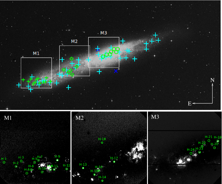
Figure 1: Top: HSDSS IIIaJ4680Å image of NGC 55. The entire image is 30$\times$15 arcmin², and it is centred at RA=00:15:12.27 and DEC=-39:12:57.89. Superposed to it the three GMOS-S FoV we observed (masks M1, M2 and M3), of 5.5$\times$5.5 arcmin² each, are highlighted. The green symbols (plus, diamond and circle) are our H ii regions located within these three FoV, respectively. Other symbols are as follows: cyan plus, the X-rays sources up to D₂₅ from Stobbart, Roberts & Warwick (2006); and the two blue crosses indicate the extra-planar H ii regions studied by Tüllmann et al. (2003). Bottom: Our GMOS-S continuum subtracted images (H$\alpha$-H$\alpha$C) of the three FoV. The H ii regions we discuss in this paper are identified, following the IDs of Table 2. The orientation, North to the top and East to the left is the same in all the panels.

Table 2: GMOS-S mask identification, classification and coordinates of the H$\alpha$ line-emitters selected from the GMOS-S pre-imaging. M1, M2 and M3 stands for the masks ID. The object classification shown is based on the follow-up spectroscopic analysis of the present study.

MaskId	Field-ID	Class	RA	Dec
			J2000.0	J2000.0
M1S1	H-1	HIIr	00:16:14.93	-39:15:51.62
M1S4	H-2	HIIr	00:16:10.12	-39:16:11.49
M1S5	NGC 55 StSy-1	SySt	00:16:07.25	-39:16:31.91
M1S6	H-3	HIIr	00:16:07.99	-39:15:45.94
M1S7	H-4	HIIr	00:16:05.73	-39:16:42.96
M1S8	H-5	HIIr	00:16:02.59	-39:15:52.35
M1S10	H-6	HIIr	00:16:03.96	-39:16:26.61
M1S12	H-7	HIIr	00:16:01.04	-39:15:42.52
M1S13	H-8	HIIr	00:15:56.26	-39:16:25.79
M1S15	H-9	HIIr	00:15:53.42	-39:15:41.12
M1S16	H-10	HIIr	00:15:59.58	-39:16:37.63
M1S17	H-11	HIIr	00:15:54.64	-39:16:25.90
M1S18	H-12	HIIr	00:15:49.66	-39:16:23.08
M2S1	H-13	HIIr	00:15:36.94	-39:14:21.08
M2S2	NGC 55 SySt-2	SySt	00:15:39.02	-39:14:40.60
M2S3	H-14	HIIr	00:15:29.36	-39:15:18.69
M2S5	H-15	HIIr	00:15:32.49	-39:14:50.50
M2S6	H-16	HIIr	00:15:30.75	-39:14:32.54
M2S14	H-17	HIIr	00:15:24.71	-39:13:51.88
M2S15	H-18	HIIr	00:15:29.41	-39:12:25.09
M3S1	H-19	HIIr	00:14:46.02	-39:11:01.79
M3S2	H-20	HIIr	00:14:47.32	-39:11:32.85
M3S3	H-21	HIIr	00:14:49.52	-39:10:59.99
M3S4	H-22	HIIr	00:14:52.18	-39:11:26.70
M3S5	H-23	HIIr	00:14:53.18	-39:11:53.30
M3S7	H-24	HIIr	00:14:56.52	-39:11:58.05
M3S8	NGC 55 StSy-3	SySt	00:14:58.61	-39:11:59.14
M3S10	H-25	HIIr	00:14:59.94	-39:12:14.97

The data analysed in the present paper were obtained with the Gemini Multi-Object Spectrographs (GMOS) at Gemini South telescope in 2012 and 2013. The two programs through which the data were taken are GS-2012B-Q-10 and GS-2013B-Q-12, with D. R. Gonçalves as Principal Investigator (PI) in both cases. In total we observed three fields of view of GMOS-S, each of 5.5′$\times$5.5′. In the following, we refer to the three fields as M1, M2 and M3 (see Figure  1).

Pre-Imaging

We obtained the pre-imaging of NGC 55 with the GMOS-S camera in queue mode on the 28^th (M1) and 27^th (M2, M3) of August 2012. We used the on- and off-band imaging technique to identify the strongest H$\alpha$ line emitters. Their location is shown in Figure 1. For the three fields of view (FoV) the on-band H$\alpha$ images were sub-divided in 3 exposures of 60 s each, while the three off-band (the continuum of H$\alpha$) H$\alpha$C sub-exposures were of 120 s each. These narrow-band filters have central $\lambda$ ($\lambda$ interval) of 656nm (654-661nm) and 662nm (659-665nm) for H$\alpha$ and H$\alpha$C, respectively. The location of the three fields (5.5′$\times$5.5 ′) is shown in Figure 1, and the central coordinates of each field are: for M1 R.A. 00:16:02.62 and Dec. -39:14:41.77; for M2 R.A. 00:15:26.59 and Dec. -39:12:49.08; and for M3 R.A. 00:14:59.06 and Dec. -39:11:30.97. During the pre-imaging observations, the seeing varied from 0.9” to 1$\aas@@fstack{\prime\prime}$0.

In Table 2 we give the coordinates of the observed emission-line objects (25 H ii regions, HIIr, and 3 candidate symbiotic systems, SySt). We based the classification of the nebulae on the analysis of their spectra, which will be introduced in the following sections. We discriminate SySts from H ii regions on the bases of the presence of absorption features and continuum of late-type M giants, of the strong nebular emission lines of Balmer H i, He ii, the simultaneous presence of forbidden lines of low- and high-ionization, like [O ii], [Ne iii], [O iii]  (Belczyński et al., 2000) and of the Raman scattered line at $\lambda$6825Å, a signature almost exclusively seen in symbiotic stars (Schmid, 1989; Belczyński et al., 2000).

In Figure 1 the positions of our H ii regions are shown in contrast with objects investigated in previous works: X-rays sources up to D₂₅ from Stobbart, Roberts & Warwick (2006); and the extra-planar H ii regions from Tüllmann et al. (2003).

Spectroscopy

The spectroscopic observations were obtained in queue mode with two gratings, R400+G5305 (red) and B600 (blue). For the mask M1, the spectra were taken on the 22^nd (blue) and 23^th (red) of December 2012. The spectroscopy of M2 and M3, on the other hand, were obtained about one year later. The red spectra of M2 on the 29^th of September, while the blue counterpart was observed on the 13^th of October, in 2013. As for M3, the red and blue spectra were taken on the nights of 27^th and 29^th of December of 2013.

We obtained three exposures per mask and grating –with 3$\times$1,430s for M1 and 3$\times$1,390s for M2 and M3 both in blue and red. For technical reasons, only one exposure of the blue spectra of M3 and two of the red spectra of M2 were useful for science. In all the cases, we combined the good quality exposures to increase the signal-to-noise ratio (SNR) of the spectra and to remove cosmic rays.

For most of the spectra the effective blue plus red spectral coverage range from 3500 Å to 9500 Å, in several cases allowing a significant overlap of the spectra. Only few lines were measured with wavelength longer than  7200 Å, because of the poor (wavelength + flux) calibration at the red end of the spectra (see Figure 2). We avoided the possibility of important emission-lines to fall in the gap between the three CCDs, by slightly varying the central wavelength of the disperser from one exposure to another. To do this, we centred the red grating R400+G5305 at 750 $\pm 10$ nm and the blue one B600 at 460 $\pm 10$ nm.

The masks were built with slit widths of 1^′′ and with varying lengths to include portions of sky in each slit for a proper local sky-subtraction. The spectroscopic observations were spatially$\times$spectrally binned. The final spatial scale and reciprocal dispersions of the spectra were: 0$\aas@@fstack{\prime\prime}$144 and 0.09 nm per pixel, in blue; and 0$\aas@@fstack{\prime\prime}$144 and 0.134 nm per pixel, in red.

Following the usual procedure with GMOS for wavelength calibration, we obtained CuAr lamp exposures with both grating configurations, either the day before and after the science exposures. The spectrophotometric standard LTT7379 (Hamuy et al., 1992) was observed with the same instrumental setups as for science exposures, on September 2^nd 2013, and used for flux calibration of the three masks, since no standards were obtained near the observation of M1, in 2012. In Figure 2 we show a sample with fully reduced and calibrated GMOS spectra, one spectrum per field, on which it is straightforward to see the quality of our data.

Data were reduced and calibrated in the standard way by using the Gemini gmos data reduction script and long-slit tasks, both being part of IRAF

3 Spectral analysis and determination of the physical and chemical properties

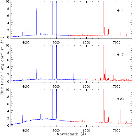
Figure 2: Sample of our GMOS spectra, one per FoV, M1, M2 and M3, for the H ii regions H-11, H-17 and H-23, respectively. The CCD gaps in the blue part of H-23’s spectrum were masked, since in this case only one spectrum was good enough for science, so the CCD gaps could not be erased by the combination of different frames. Also note the red spectrum of H-17, noisier than in of the other two H ii regions due to the fact that 2, instead of 3 spectra were combined to obtain this one.

We measured the emission-line fluxes and their errors with the package SPLOT of IRAF. Errors take into account the statistical errors in the measurement of the fluxes and the systematic errors (flux calibrations, background determination and sky subtraction).

We corrected the observed line fluxes for the effect of the interstellar extinction using the extinction law of Mathis (1990) with R_V=3.1 (which is assumed to be constant as in our Galaxy, but might slightly vary from galaxy to galaxy, see, e.g., Clayton et al. (2015)) and the individual reddening of each H ii region given by the $c_{\beta}$, i.e., the logarithmic difference between the observed and theoretical H$\beta$ fluxes. Since H$\delta$ and H$\gamma$ lines are fainter than the H$\alpha$ and H$\beta$ ones, and located in the bluer part of the spectra, they are consequently affected by larger uncertainties. We thus determined $c_{\beta}$ comparing the observed Balmer I(H$\alpha$)/I(H$\beta$) ratio with its theoretical value, 2.87 (case B. c.f., Osterbrock & Ferland, 2006). We used lines in common between the blue and red part of the spectra to put the two spectral ranges on the same absolute flux scale. The average scaling factor applied to the fluxes of the red spectra is 0.78.

In Table B1 of the Appendix we present the measured and extinction corrected intensities –both normalised to H$\beta$=100– of the emission lines of the 25 H ii regions listed in Table 2. The spectra of the candidate symbiotic systems will be discussed in a forthcoming paper.

The method to derive the physical and chemical condition in H ii regions is described in the previous papers of this series, as for instance Magrini & Gonçalves (2009); Gonçalves et al. (2012, 2014): the temden and ionic tasks of IRAF are used to derive first electron temperature (from the ratio of the [O iii] lines at 500.7 nm and 436.3 nm), and density (from the lines of the [S ii] doublet at 671.7 nm and 673.1 nm) of the gas, then ionic abundances. Ionic abundances are combined with the ionisation correction factors for H ii regions from Izotov et al. (2006) to obtain the total abundances.

Often, literature studies represent H ii regions with a two-zone ionisation structure characterised by two different electron temperature, for the [O ii] and [O iii] emitting regions. If available $T_{e}$[O II] –or equivalently $T_{e}$[N II] – are used for the [O ii] zone, while $T_{e}$[O III] is adopted in the [O iii] emitting zone. When $T_{e}$[O II] or $T_{e}$[N II] are not measured, the relation, based on the photoionisation models of Stasińska (1982), $T_{e}$[O II]=0.7$\times$$T_{e}$[O III]+3000 K (or a similar one) is adopted. If we consider valid without errors the linear relation between $T_{e}$[O II] and $T_{e}$[O III], in the temperature range of our H ii regions, the use of a single temperature (the measured one, i.e., $T_{e}$[O III]) might imply a maximum underestimation of about $\sim$700 K and up to a maximum overestimation of $\sim$400 K of the temperature adopted for the [O ii] ionic abundance. We have tested the effect of adopting two different temperatures and, for most regions, it has negligible effect on the total oxygen abundance –of the order 0.01-0.03 dex– since [O iii] ionic abundance is on average a factor 10 larger than [O ii] ionic abundance, and consequently it is the ionic fraction that contributes the most to the total O/H. Thus we use only the measured $T_{e}$[O iii]  for the calculation of the abundances of both low- and high-ionisation species.

The abundances of He i and He ii were computed using the equations of Benjamin et al. (1999) in two density regimes, that is $N_{e}$ $>$ 1,000 and $\leq$ 1,000 cm^-3. Clegg’s collisional populations were taken into account (Clegg, 1987).

The results of physical and chemical properties of the H ii regions are shown in Table 4. The $T_{e}$ has been measured in 18 regions and ranges from 8,600 to 12,000 K; $N_{e}$ is available in 10 regions, while an upper limit is measured in other 6 regions. The measurements of electron densities range from 100 to 600 cm^-3, typical values of H ii regions, with a higher density of 1400 cm^-3 in H-13. Errors on final abundances take into account the errors on $T_{e}$  on $N_{e}$ and on the line fluxes. The average oxygen abundance determined with the $T_{e}$ method, excluding lower limit abundances, is 12+$\log$(O/H)=8.13$\pm$0.18. For the other elements we obtain average values: 12+$\log$(N/H)=7.18$\pm$0.28, 12+$\log$(Ne/H)=6.81$\pm$0.14, 12+$\log$(Ar/H)=6.00$\pm$0.25, and 12+$\log$(S/H)=6.04$\pm$0.25. Helium abundance is quite uniform too. Its mean value, linearly expressed, is He/H=0.092$\pm$0.019. The mean O/H is in good agreement with the metallicity measured by Tüllmann et al. (2003) in their H ii region located in the disc-halo transition of NGC 55 (8.05$\pm$0.10 with the $T_{e}$-method). The two extra-planar H ii regions of Tüllmann et al. (2003) are instead slightly metal poorer (7.77 and 7.81) than our average O/H, but they are still consistent with the composition of some individual H ii regions, as for instance H-19, H-20, H-21. This might be an indication of incomplete mixing in the disc of NGC 55.

Table 3: Electron temperatures, electron densities, ionic and total abundance of the H ii regions.

Diagnostic	H-1	H-2	H-5	H-6	H-7	H-11	H-12	H-13	H-14
$T_{e}$[O iii](K)	12000$\pm$200	9200$\pm$150	9300$\pm$150	11500$\pm$200	12000$\pm$200	8700$\pm$150	11000$\pm$200	10700$\pm$200	10800$\pm$200
$N_{e}$ [S ii](cm-3)	-	$<100$	100$\pm$50	$<100$	200$\pm$50	$<$100	600$\pm$100	1400$\pm$200	250$\pm$50
He i/H	0.14	0.07	0.09	0.07	0.11	0.10	0.075	0.07	0.10
He/H	0.14$\pm$0.03	0.07$\pm$0.01	0.09$\pm$0.01	0.07$\pm$0.01	0.11$\pm$0.05	0.10$\pm$0.05	0.075$\pm$0.05	0.07$\pm$0.02	0.10$\pm$0.05
O ii/H	2.1e-06	3.2e-05	1.9e-05	5.4e-05	1.4e-05	6.1e-05	2.2e-05	-	1.6e-05
O iii/H	1.3e-04	1.1e-04	1.5e-04	1.9e-05	7.9e-05	2.0e-04	1.1e-04	8.9e-05	9.8e-05
ICF(O)	1.2	1.0	1.0	1.0	1.0	1.0	1.0	-	1.0
O/H	1.6e-04	1.4e-04	1.7e-04	3.5e-05	9.3e-05	2.6e-04	1.3e-04	$>$8.9e-05	1.1e-04
12+log(O/H)	8.21$\pm$0.07	8.15$\pm$0.06	8.23$\pm$0.06	7.90$\pm$0.10	7.97$\pm$0.12	8.42$\pm$0.12	8.12$\pm$0.08	$>$7.95	8.06$\pm$0.07
N ii/H	8.9e-07	3.5e-06	2.8e-06	3.9e-06	1.5e-06	2.9e-06	1.4e-06	1.17e-06	2.2e-06
ICF(N)	45.0	4.5	7.6	1.6	6.2	4.4	5.5	-	6.5
N/H	3.9e-05	1.5e-05	2.1e-05	6.2e-06	9.2e-06	1.2e-05	7.6e-06	-	7.7e-05
12+log(N/H)	7.58$\pm$0.15	7.18$\pm$0.15	7.32$\pm$0.15	6.80$\pm$0.15	6.96$\pm$0.12	7.10$\pm$0.15	6.88$\pm$0.12	-	7.16$\pm$0.12
Ne iii/H	5.1e-06	4.7e-06	5.5e-06	-	1.0e-05	8.0e-06	5.2e-06	-	8.1e-06
ICF(Ne)	1.0	1.2	1.0	-	1.1	1.2	1.1	-	1.0
Ne/H	5.1e-06	5.5e-06	5.5e-06	-	1.1e-05	9.5e-06	5.7e-06	-	8.5e-06
12+log(Ne/H)	6.70$\pm$0.14	6.74$\pm$0.15	6.75$\pm$0.15	-	7.03$\pm$0.04	6.7$\pm$0.14	6.76$\pm$0.14	-	6.93$\pm$0.15
Ar iii/H	-	9.4e-07	8.8e-07	2.9e-07	5.4e-07	1.4e-06	7.5e-07	-	-
ICF(Ar)	-	1.1	1.2	1.2	1.1	1.1	1.1	-	-
Ar/H	-	1.0e-06	1.0e-06	3.5e-07	6.0e-07	1.5e-06	8.2e-07	-	-
12+log(Ar/H)	-	6.00$\pm$0.20	6.00$\pm$0.20	5.53$\pm$0.20	5.78$\pm$0.22	6.20$\pm$0.25	5.90$\pm$0.23	-	-
S ii/H	-	1.2e-06	8.5e-07	7.2e-07	3.4e-07	8.7e-07	4.2e-07	2.4e-07	6.3e-07
S iii/H	-	-	-	-	5.1e-07	-	-	-	-
ICF(S)	-	1.3	2.0	1.0	1.7	1.3	1.5	-	1.7
S/H	-	1.6e-06	1.7e-06	7.2e-07	1.4e-06	1.2e-06	6.5e-07	-	1.1e-06
12+log(S/H)	-	6.19$\pm$0.30	6.22$\pm$0.30	5.90$\pm$0.30	6.16$\pm$0.28	6.10$\pm$0.30	5.80$\pm$0.30	-	6.05$\pm$0.30

Table 4: continued

Diagnostic	H-15	H-17	H-18	H-19	H-20	H-21	H-22	H-23	H-25
$T_{e}$[O iii](K)	8600$\pm$150	10000$\pm$150	12000$\pm$500	12000$\pm$200	12400$\pm$300	10500$\pm$200	9900$\pm$150	9100$\pm$150	9600$\pm$150
$N_{e}$ [S ii](cm-3)	100$\pm$50	$<$100	-	300$\pm$100	150$\pm$50	$<$100	$<$100	150$\pm$50	200$\pm$50
He i/H	0.075	0.07	0.10	0.08	0.10	0.09	0.095	0.094	0.115
He/H	0.075$\pm$0.02	0.07$\pm$0.02	0.10$\pm$0.05	0.075$\pm$0.02	0.07$\pm$0.02	0.09$\pm$0.01	0.095$\pm$0.01	0.094$\pm$0.01	0.115$\pm$0.03
O ii/H	2.6e-05	4.2e-05	-	2.0e-06	1.3e-05	1.5e-05	1.0e-05	1.6e-05	4.2e-06
O iii/H	2.1e-04	1.1e-04	1.7e-04	9.1e-05	6.0e-05	4.2e-05	1.3e-04	1.6e-04	2.4e-04
ICF(O)	1.0	1.0	-	1.0	1.0	1.0	1.0	1.0	1.0
O/H	2.3e-04	1.6e-04	$>$1.7e-04	9.3e-05	7.3e-05	5.7e-05	1.4e-04	1.8e-04	2.4e-04
12+log(O/H)	8.36$\pm$0.12	8.20$\pm$0.07	$>$8.25	7.70e$\pm$0.12	7.86$\pm$0.13	7.80$\pm$0.12	8.16$\pm$0.08	8.25$\pm$0.08	8.38$\pm$0.12
N ii/H	-	3.8e-06	-	3.9e-07	1.4e-06	3.0e-06	2.6e-06	1.9e-06	1.9e-06
ICF(N)	-	4.0	-	34.2	5.4	4.0	11.4	9.1	41.4
N/H	-	1.4e-05	-	1.5e-05	7.2e-06	1.2e-05	2.9e-05	1.6e-05	7.7e-05
12+log(N/H)	-	7.17$\pm$0.20	-	7.10$\pm$0.13	6.86$\pm$0.10	7.10$\pm$0.12	7.46$\pm$0.15	7.22$\pm$0.10	7.88$\pm$0.20
Ne iii/H	6.9e-06	7.9e-06	-	4.8e-06	3.8e-06	-	5.0e-06	8.6e-06	7.8e-06
ICF(Ne)	1.2	1.2	-	1.0	1.1	-	1.0	1.0	1.0
Ne/H	7.1e-06	9.8e-06	-	4.8e-06	4.2e-06	-	5.0e-06	8.6e-06	7.8e-06
12+log(Ne/H)	6.85$\pm$0.14	7.00$\pm$0.14	-	6.66$\pm$0.15	6.62$\pm$0.14	-	6.70$\pm$0.15	6.93$\pm$0.15	6.89$\pm$0.15
Ar iii/H	-	7.2e-07	-	4.6e-07	6.0e-07	8.7e-07	-	1.4e-06	1.2e-06
ICF(Ar)	-	1.1	-	2.8	1.1	1.1	-	1.3	3.2
Ar/H	-	7.6e-07	-	1.3e-06	6.6e-07	9.2e-07	-	1.8e-06	3.9e-06
12+log(Ar/H)	-	5.88$\pm$0.24	-	6.10$\pm$0.17	5.82$\pm$0.23	6.00$\pm$0.24		6.26$\pm$0.17	6.59$\pm$0.23
S ii/H	7.3e-07	5.3e-07	-	9.8e-08	3.0e-07	6.2e-07	4.6e-07	3.0e-07	6.1e-07
ICF(S)	2.0	1.2		7.8	1.5	1.2	2.8	2.3	9.4
S/H	1.5 e-06	6.5e-07	-	7.7e-07	4.5e-07	7.8e-07	1.3e-06	6.9e-07	5.8e-06
12+log(S/H)	6.20$\pm$0.30	5.80$\pm$0.30	-	5.90$\pm$0.30	5.65$\pm$0.30	5.90$\pm$0.30	6.11$\pm$0.27	5.84$\pm$0.27	6.76$\pm$0.30

3.1 Strong-line metallicities

We computed oxygen abundances using strong-line methods to increase the number of regions with a determined metallicity. These methods are based on the intensities of lines that are usually easy to measure because they are much stronger than the lines used as $T_{e}$ diagnostic (c.f. Arellano-Córdova et al., 2015, for a complete discussion and comparison among the methods). The strong-line ratios can be calibrated in two different ways: using photoionisation models or using abundances of H ii regions obtained through the $T_{e}$-method. Since the empirical calibration works better in the low metallicity regime, we have used the new calibrations based on $T_{e}$-method abundances by Marino et al. (2013, hereafter M13) of the two well-known indices, N2=$\log$([N ii]/H$\alpha$) and O3N2=$\log$[([O iii]/H$\beta$)([N ii]/H$\alpha$)]. The results are shown in Table 5 where we present the galactocentric distances, O/H from the $T_{e}$-method, the metallicities derived with the M31’s N2 and O3N2 indices, and an average between the two strong-line calibrators, which is the value adopted in the following figures. Errors on the adopted strong-line O/H take into account the flux uncertainties and the intrinsic errors of the method (0.18 and 0.16 dex, for O3N2 and N2, respectively, as quoted in M13).

Comparing the average oxygen abundance derived with the $T_{e}$-method, 12+$\log$(O/H)=8.13$\pm$0.18, with the average values determined with the strong-line method, we have: for the N2 index 12+$\log$(O/H)=8.14$\pm$0.12, for the O3N2 index 12+$\log$(O/H)=8.20$\pm$0.14, and for the combination of the two indices 12+$\log$(O/H)=8.17$\pm$0.13. They are thus in extremely good agreement. The increment of the number of regions analysed with the strong-line methods provides an even smaller dispersion of the distribution of the abundances in NGC 55 pointing towards a very homogeneous composition for the interstellar medium for this galaxy.

Table 5: Strong-line calibrated oxygen abundances.

Field-ID	D	O/H	O/H	O/H	O/H
	kpc	Te	N2	O3N2	adopted
			M13	M13
H-1	12.13${}^{+0.45}_{-1.35}$	8.21$\pm$0.07	8.03	7.97	8.03$\pm$0.21
H-2	10.90${}^{+0.14}_{-0.45}$	8.15$\pm$0.06	8.14	8.18	8.16$\pm$0.21
H-3	10.84${}^{+0.27}_{-0.84}$	-	8.18	8.27	8.22$\pm$0.30
H-4	10.21${}^{+0.00}_{-0.00}$	-	8.30	8.57	8.43$\pm$0.21
H-5	9.87${}^{+0.10}_{-0.32}$	8.23$\pm$0.06	8.10	8.13	8.12$\pm$0.21
H-6	9.01${}^{+0.00}_{-0.01}$	7.90$\pm$0.10	8.25	8.32	8.28$\pm$0.22
H-7	9.43${}^{+0.09}_{-0.29}$	7.97$\pm$0.12	8.11	8.13	8.12$\pm$0.25
H-8	9.01${}^{+0.05}_{-0.17}$	-	8.26	8.37	8.32$\pm$0.21
H-9	8.42${}^{+0.00}_{-0.02}$	-	8.12	8.14	8.13$\pm$0.23
H-10	9.52${}^{+0.03}_{-0.11}$	-	8.27	8.44	8.31$\pm$0.21
H-11	8.93${}^{+0.07}_{-0.23}$	8.42$\pm$0.12	8.12	8.14	8.13$\pm$0.21
H-12	8.55${}^{+0.19}_{-0.59}$	8.12$\pm$0.08	8.01	8.09	8.05$\pm$0.21
H-13	6.21${}^{+0.06}_{-0.21}$	$>$7.95	8.00	8.08	8.04$\pm$0.21
H-14	6.46${}^{+0.50}_{-1.41}$	8.06$\pm$0.07	8.07	8.11	8.09$\pm$0.22
H-15	5.77${}^{+0.08}_{-0.24}$	8.36$\pm$0.12	-	-	-
H-16	5.40${}^{+0.02}_{-0.07}$	-	8.22	8.21	8.21$\pm$0.21
H-17	4.42${}^{+0.00}_{-0.01}$	8.20$\pm$0.07	8.12	8.18	8.15$\pm$0.22
H-18	7.63${}^{+1.21}_{-3.03}$	$>$8.25	-	-	-
H-19	1.46${}^{+0.18}_{-0.46}$	7.70$\pm$0.12	7.83	7.99	7.91$\pm$0.21
H-20	0.95${}^{+0.06}_{-0.18}$	7.86$\pm$0.13	8.10	8.16	8.13$\pm$0.22
H-21	2.12${}^{+0.52}_{-1.17}$	7.80$\pm$0.12	-	-	-
H-22	1.00${}^{+0.25}_{-0.56}$	8.16$\pm$0.08	8.13	8.13	8.13$\pm$0.21
H-23	0.28${}^{+0.08}_{-0.16}$	8.25$\pm$0.08	8.00	8.09	8.05$\pm$0.21
H-24	0.43${}^{+0.01}_{-0.03}$	-	8.27	8.25	8.26$\pm$0.22
H-25	0.98${}^{+0.00}_{-0.00}$	8.38$\pm$0.12	8.05	8.05	8.05$\pm$0.21

4 Radial abundance gradients in NGC 55

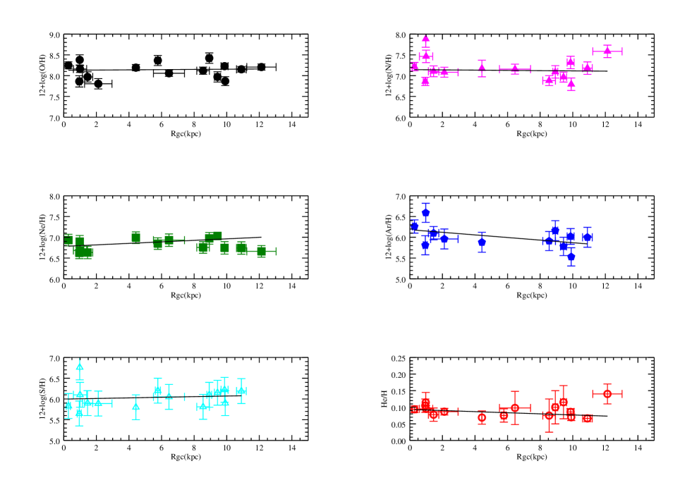
Figure 3: Radial abundance gradients of elemental abundances in the H ii regions in NGC 55. The abundances of metals (O, N, Ne, Ar, S) are expressed in the logarithmic form 12$+\log$(O/H), whereas the abundance of helium is expressed in linear form. The continuous curves are the weighted linear fits to the data, taking into account errors on both distances and abundances.

Table 6: Radial abundance gradients in the disc of NGC 55

El.	Slope	Intercept
O/H	+0.0025$\pm$0.0055	8.13$\pm$0.04
Ne/H	+0.0181$\pm$0.0081	6.78$\pm$0.06
N/H	-0.0030$\pm$ 0.0082	7.14$\pm$0.06
Ar/H	-0.0313$\pm$0.0145	6.18$\pm$0.10
S/H	+0.0074$\pm$0.0196	5.99$\pm$0.13
He/H	-0.0017$\pm$0.0008	0.094$\pm$0.006
N/O	-0.0103$\pm$0.0103	-0.880$\pm$0.074

The H ii regions for which we can determine plasma conditions, including $T_{e}$, $N_{e}$, ionic and total abundances, give us the opportunity to study the spatial distribution of abundances and abundance ratios of several elements in the thin/thick disc of NGC 55. We have computed the linear galactocentric distances de-projecting and transforming them in linear distances with the inclination, position angle and distance of Table 1. We use the range of 4^∘ in the inclination angle obtained by the disc model of Puche, Carignan & Wainscoat (1991) to estimate the uncertainties in de-projected galactocentric distance. The new model of Westmeier et al. (2013) is consistent with the one of Puche in the inner part of the galaxy where our regions are located.

The sample of H ii regions (see green symbols in Figure 1) are located in a large galactocentric range of distances (from the centre to about 12 kpc, see Table 5).

In Figure 3 we show the radial abundance gradients of several elements: O, Ne, S, Ar, N and He. In Table 6 we report the slopes and the intercepts of the radial abundance gradients computed with the fitexy routine that takes into account both the errors on abundances and galactocentric distances. For all the available elements we found null gradients, within the errors.

NGC 55 radial gradients of O/H and N/H have been also recently re-analysed from literature data by Pilyugin et al. (2014). They found oxygen and nitrogen gradients essentially flat, and in good agreement with our results (see Table6). Their slopes for oxygen and nitrogen are -0.0059$\pm$0.0104 dex kpc^-1 and -0.0042$\pm$ 0.0145 dex kpc^-1, respectively. On the other hand, Kudritzki et al. (2016) analysed a sample of 58 blue supergiant stars. For the first time, they detected a non negligible metallicity gradient of -0.22$\pm$0.06 dex/R₂₅ (-0.020$\pm$0.005 dex kpc^-1 assuming R₂₅=11.0 kpc). Their central metallicity relative to the Sun is Z=-0.37$\pm$0.03.

The comparison between the H ii region and blue supergiant populations is extremely interesting because they both are young populations and should trace the same epoch in the galaxy lifetime. In the upper panel of Figure 4 we plotted the metallicity of the supergiants of Kudritzki et al. (2016) and of our H ii regions –reported on the Solar scale (12+$\log$(O/H)=8.66; Grevesse et al., 2007)– versus the galactocentric distance. We have plotted the whole sample of Kudritzki et al. (2016) without removing the possible outliers. The two sets of metallicities and their radial distributions are in surprisingly good agreement considering all the internal uncertainties of the two metallicity derivations, the differences in the metallicities measured from nebular and stellar spectra (oxygen in the former, a global Z metallicity in the latter), and possible dust depletion of oxygen in H ii regions (this correction might amount to 0.10 dex for objects with 7.8$<$12+$\log$(O/H)$<$ 8.3); see Peimbert & Peimbert, 2010). It is, however, true that the supergiant abundances show a small decreasing gradient, which is not appreciable in the H ii region population abundances.

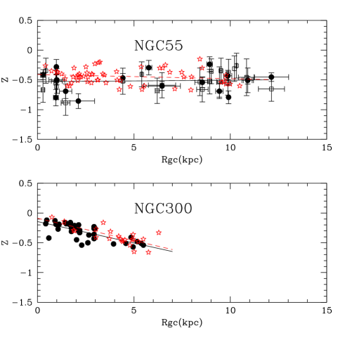
Figure 4: Upper panel: NGC 55 H ii regions (O/H derived with the $T_{e}$ method –filled circles– and from the strong-line method –empty squares. For the strong-line abundances we adopted the average of the two values, as indicated in Table 5) and supergiants from Kudritzki et al. (2016) (empty stars) radial distribution. The continuous line is the fit to the H ii regions with $T_{e}$ determinations as in Figure 3, whereas the dotted line is the fit to the whole sample of supergiant abundances. Lower panel: NGC 300 H ii regions (Bresolin et al., 2009; Stasińska et al., 2013, filled circles from) and supergiants from Kudritzki et al. (2008) (empty stars) radial distribution.

4.1 $\alpha$-elements and nitrogen

Giving the similar origin of the four $\alpha$-elements –O, Ne, S and Ar– we expect them to have similar radial behaviours. We indeed find almost flat gradients within the uncertainties for all of them, with Ar having possibly a small negative slope, still consistent with a null gradient, within the errors.

While $\alpha$-elements are mainly synthesised by massive stars (M$>$8 M_⊙), nitrogen has a more complex nucleo-genesis, having both a “primary” and a “secondary” origin. The primary origin refers to conversion of the original hydrogen into nitrogen and it happens in stars with 4 M${}_{\odot}<$M$<$8 M_⊙ (Renzini & Voli, 1981) and/or in very massive (M$>$30M_⊙) low metallicity stars (Woosley & Weaver, 1995), while the secondary channel is related with the production from C and O initially present in the ISM at the formation of the progenitor star. When the primary nitrogen component dominates, the N/O ratio is expected to be independent of the oxygen abundance and this happens at low metallicity. At higher metallicity, the secondary production becomes more important, and N/O increases with O (van Zee et al., 1998).

The comparison of N with any $\alpha$-element can give indication on different star formation history in different radial regions of NGC 55 disc. If a galaxy experiences a dominant global burst of star formation, the ISM oxygen abundance will increase in about 10⁶ yr, generating a decrease in N/O. Then over a period of several 100$\times$10⁶ yr N/O will increase at constant O/H. Consequently N/O can be used as a clock that measures the time since the last major burst of star formation: low values of N/O imply a very recent burst of star formation, while high values of N/O imply a long quiescent period (cf. Skillman, 1998). In Figure 5, the radial gradient of N/O is shown. A slightly decreasing gradient towards the outskirts is detected. However this gradient is consistent with 2-$\sigma$ with a flat gradient and homogeneous distribution of abundances, indicating no differences in the star formation histories in different parts of the galaxy. We can also compare the typical N/O value in NGC 55 with those of dwarf and spiral star forming galaxies. From Figure 5 of Pilyugin et al. (2003) or Figure 7 of Annibali et al. (2015) we can infer that at 12$+\log$O/H$\sim$8.0 dex, there is an increasing dispersion in N/O, with values ranging from $-$1.6 to $-1$ dex. N/O in NGC 55 is located towards the upper envelope of this relationship. The average N/O of NGC 55 (N/O$=-$0.93$\pm$0.21) is close to the M33’s one (see, e.g., Figure 12 in Magrini et al. 2007, for a plot of N/O vs O/H) and to that of the LMC (N/O=-0.96; Carlos Reyes et al., 2015). The scatter in N/O values at a given O/H seen, e.g., by Pilyugin et al. (2003) and Annibali et al. (2015), can be naturally explained by differences in the star formation histories of galaxies (Pilyugin et al., 2003). This conclusion was already suggested by Edmunds & Pagel (1978) who explained the observations of the N/O abundance ratio in external galaxies due to the manufacturing of N in low-mass stars of 4-8 M_⊙. Very recently, Vincenzo et al. (2016) presented chemical evolution models aimed at reproducing the observed N/O versus O/H abundance pattern of star-forming galaxies in the Local Universe. They found that position of a galaxy in the N/O vs. O/H plane is mostly determined by its star formation efficiency (see their Figure 4). The high N/O ratio in NGC 55 with respect to other late-type dwarf irregular galaxies having the same O/H might be an indication that the bulk of the star formation happened in the recent past, more than 100$\times$10⁶ yr ago. This is in agreement with the finding of Davidge (2005) of a vigorous star formation episode during the past 0.1-0.2 Gyr. The detection of significant numbers of stars evolving on the AGB phase, indicates that there has been vigorous star formation during the past 0.1-0.2 Gyr. In this time lapse, stars with masses M$>$5 M_⊙ might had time to evolve and to pollute with N the ISM of NGC 55 and thus to increase the N/O ratio.

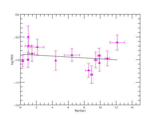
Figure 5: Radial N/O gradients of H ii regions of NGC 55.

4.2 Helium

The measurement of He in low metallicity galaxies has been often used to extrapolate the primordial He abundance. To account for the amount of helium synthesised by stars, Peimbert & Torres-Peimbert (1974) suggested for the first time to study a sample of H ii regions spanning a wide range of metallicity. With the assumption of a helium enrichment proportional to metallicity, we can obtain the primordial abundance of He extrapolating to zero metallicity:

$$Y=Y_{\rm P}+Z(\Delta Y/\Delta Z),$$

where Y is the mass fraction of He, and Z is the metallicity. Using Equation 2 of Izotov et al. (1997) without correction for the neutral He ($<$2%, cf. Izotov et al., 1997), we computed the mass fraction of He using the mean abundance of NGC 55, obtaining Y=0.27$\pm$0.08. Excluding the H ii region with the highest He abundance (H-1) we have a mean He/H=0.088$\pm$0.020 and thus Y=0.26$\pm$0.04. The linear regression of Izotov et al. (1997) of Y versus oxygen, computed at the metallicity of NGC 55 gives a slightly lower value Y=0.250$\pm$0.002, but still consistent within the errors with our determination. The measurement of He abundance in NGC 55 does not give any particular constraint to the primordial He abundance, but it is in line with the determination of Y in several low metallicity galaxies.

5 Discussion

NGC 55 has both been classified as an irregular and a spiral galaxy. However, although its morphology cannot be well defined because of its inclination, it is a very extended object and with a large total mass (see Table 1); its H ii regions are found up to 11-12 kpc from the centre, and its blue and red supergiants even much farther (Kudritzki et al., 2016). So, the questions are: how can the composition of its H ii regions (and supergiants) be so homogeneous in such a wide region, extending from the centre to about $\sim$11-12 kpc? Why is not there a clear metallicity gradient from the H ii region abundances?

The presence of metallicity gradients in irregular galaxies has been, indeed, deeply investigated in the literature reaching the conclusion that most of these galaxies show a spatial homogenous composition (e.g., Kobulnicky & Skillman, 1997; Croxall et al., 2009; Magrini & Gonçalves, 2009; Haurberg et al., 2013; Lagos & Papaderos, 2013; Hosek et al., 2014; Patrick et al., 2015). There are some exceptions, such as, for instance, the observed oxygen gradient in NGC 6822 (Venn et al., 2004; Lee et al., 2006) and in the dwarf blue compact galaxy NGC1750 (Annibali et al., 2015), or the iron gradients in the SMC, in the LMC, and in the dIrr WLM (Leaman et al., 2014). The systematic study of gradients in late-type spiral and irregular galaxies by Pilyugin et al. (2014, 2015) has shown that there is a strong correlation between the radial abundance gradient of galaxies and their surface brightness profiles. In particular, galaxies with a steep inner surface brightness profile usually present a noticeable radial abundance gradient. On the other hand, those galaxies with flat inner surface brightness profiles have shallower or null gradients. The reason of this different behaviour might be related to the presence of radial mixing of gas (through radial flows or galactic fountains): this process takes place more evidently in galaxies with a flat surface density inner profile that can readily redistribute the gas across the disc.

The comparison of metallicity distributions and surface density profiles in the galaxy pair, NGC 55 and NGC 300 (Scd for NGC 300 and barred spiral/irregular SB(s)m for NGC 55) allows us to investigate this hypothesis in detail. These two galaxies are indeed very similar in many aspects: comparable near-IR magnitudes (K=6.25 and 6.38, respectively, see Jarrett et al., 2003) and mid-infrared fluxes (see Dale et al., 2009) that point towards comparable stellar masses. However, they have different morphologies. Even more important, Kudritzki et al. (2016) have shown that their K-band radial surface profiles are also different, with NGC 300 having a strong central peak, which is instead absent in NGC 55 (see their Figure 12). The radial metallicity gradient of NGC 300 from H ii regions, studied by Bresolin et al. (2009) and re-analysed by Stasińska et al. (2013), is not negligible, and has a slope -0.068$\pm$0.009 dex kpc^-1 (with R₂₅=5.3 kpc), as well as the radial metallicity gradient of supergiants (Kudritzki et al., 2008; Gazak et al., 2015). These gradients are shown in the lower panel of Figure 4.

Thus, in the light of the discussion of Pilyugin et al. (2015), it seems that the different K-band radial surface profiles imply a different mass accretion/gas outflow in the two galaxies, with a consequent much higher re-distribution of metals in NGC 55 with respect to NGC 300. Kudritzki et al. (2016) concluded that the chemical evolution of NGC 55 is characterised by large amounts of gas outflow and infall, having one of the largest known infall rate in the Local Universe. This agrees well with the detailed morphological, kinematic and dynamic study of the neutral gas by Westmeier et al. (2013) who concluded that internal and external processes, such as satellite accretion or gas outflow have stirred up the gas disc, inducing streaming motions of the gas along the bar of NGC 55. In addition, Westmeier et al. (2013) made evident several isolated H i clouds within about 20 kpc projected distance from NGC 55. These clouds are similar to the high-velocity clouds of the Milky Way and they are a signature of on-going infall of gas and of the complex dynamics of NGC 55.

We also took advantage of the available X-rays data for NGC 55 to test the possibility that the intense star-forming events of the galaxy blow out the heavy elements, out of its disc to the galaxy halo. As detailed in Appendix A, the X-rays luminosity and SFR from the 12 of our 25 H ii regions for which data exists in the Chandra archive, are not consistent with the scenario on which the flat metallicity gradient would be justified by blow up of heavy elements due to extreme winds. Stobbart, Roberts & Warwick (2006) (their sources that are located within the optical confines of the galaxy are signed in Figure 1), studying the X-ray properties of NGC 55 using XMM-Newton observations, derived the physical properties of the soft residual disc component and found the SFR equal to 0.22 M_⊙ yr^-1 and the pressure of the hot gas (P/$k$) equal to $\sim$ 1.5$\times$10⁵ K cm^-3. This later value is similar to the pressure inferred for the interior of the Loop 1 superbubble within our Galaxy (Willingale, 2003). The authors conclude that although this is broadly consistent with the scenario where there has been sufficient recent star formation in the disc of NGC 55 to form expanding bubbles responsible for ejecting the material out of the disc into the halo, the absence of an extended extra-planar soft X-ray component in NGC 55 (contrary to what was found by Oshima, 2002) points to the fact that the gas in such bubbles cools relatively quickly through adiabatic losses, retaining insufficient energy to power a superwind of the form frequently seen in systems with SFR $>$ 1 M_⊙ yr^-1 (Strickland, 2004). So, our H ii region sample does not produce enough superwind in NGC 55, which is in agreement with previous analysis, though we should keep in mind that from all the star formation indicators, the X-ray is the weakest one.

Therefore all the above discussions suggest that the dominant effects in flattening the metallicity gradient of NGC 55 are those related to the dynamics of the gas through bar-driven mixing and inflow/outflow.

6 Conclusions

In the present paper we show new spectroscopic observations of a large sample of 25 H ii regions in the Sculptor group member galaxy, NGC 55. We derive physical and chemical properties though the $T_{e}$-method of 18 H ii regions, and strong-line abundances for 22 H ii regions. We measure also abundances of He, O, N, Ne, S, Ar. We found a homogenous composition of the disc of NGC 55, with average abundances of He/H=0.092$\pm$0.019, 12+$\log$(O/H)=8.13$\pm$0.18, 12+$\log$(N/H)=7.18$\pm$0.28, 12+$\log$(Ne/H)=6.81$\pm$0.14, 12+$\log$(Ar/H)=6.00$\pm$0.25 and 12+$\log$(S/H)=6.04$\pm$0.25. The abundances are uniformly distributed in the radial direction. This agrees with the study of smaller samples of H ii regions (Webster & Smith, 1983; Pilyugin et al., 2014) and it is in qualitative agreement with the blue supergiant radial gradient (Kudritzki et al., 2016). We investigate the origin of such flat gradient comparing NGC 55 with its companion galaxy, NGC 300, similar in terms of mass and luminosity and located in the same group of galaxies. The most plausible hypothesis is related to the differences in their K-band surface density profile that, as suggested by Pilyugin et al. (2015), which can provide higher mixing of the NGC55 gaseous component than in similar galaxies.

7 Acknowledgments

We are extremely grateful to Rolf Kudritzki for his constructive and helpful report. The work of DRG was partially supported by FAPERJ’s grant APQ5-210.014/2016. The work of Bruna Vajgel is sponsored by grants from CNPq, process number 164858/2015-6. This research has made use of data obtained from the Chandra Data Archive and software provided by the Chandra X-ray Center (CXC) in the application packages CIAO.

Appendix A X-ray Luminosity

We complemented our observations with the available X-ray observations of the H ii regions in NGC 55 in the Chandra archive.

The analysis of the X-ray emission for the 25 nebulae consists basically of measuring the source net counts and then converting the count rate into X-ray flux and luminosity. We used archival Chandra observation (ObsID 2255) with exposure of 60.1 ks of NGC 55, performed in 2001 September with the Advanced CCD Imaging Spectrometer (ACIS-I). The Chandra data were reduced and reprocessed using the science threads of Chandra Interactive Analysis of Observations (CIAO) version 4.6.

Table 7: X-ray net counts, luminosities and SFR of the H$\alpha$ line-emitters from Table 1.

Field-ID	Net Counts	Aperture	L2-10keV	SFR
	(photons)	(“)	(1036 erg s-1)	(10-3 M⊙ yr-1)
H-1	-0.33	1.5	$<$1.53	$<$0.40
H-2	-2.36	4.0	$<$10.94	$<$2.88
H-3	-0.60	2.0	$<$2.79	$<$0.73
H-4	0.67	1.5	3.11$\pm$4.64	0.82
H-5	-0.92	2.5	$<$4.26	$<$1.12
H-6	-0.32	3.0	$<$4.64	$<$1.22
H-7	1.69	3.0	7.82$\pm$8.05	2.06
H-8	-1.32	3.0	$<$6.10	$<$1.61
H-9	2.78	7.0	12.89$\pm$14.84	3.39
H-10	-0.59	2.0	$<$2.74	$<$0.72
H-11	0.22	3.5	1.02$\pm$6.58	0.27
H-12	-2.02	4.5	$<$4.64	$<$1.22
H-13	6.69	6.0	31.06$\pm$16.16	8.17
H-14	-0.33	3.0	$<$4.64	$<$1.22
H-15	-0.95	4.5	$<$9.28	$<$2.44
H-16	0.67	3.0	3.12$\pm$6.58	0.82
H-17	4.65	6.0	21.57$\pm$14.77	5.68
H-18	0.40	2.0	1.85$\pm$4.65	0.49
H-19	-0.74	10.0	$<$64.99	$<$17.10
H-20	-0.35	3.0	$<$4.64	$<$1.22
H-21	1.41	2.0	6.54$\pm$6.57	1.72
H-22	-0.35	4.0	$<$9.28	$<$0.002
H-23	2.64	4.0	12.26$\pm$10.40	3.23
H-24	0.07	2.5	0.32$\pm$4.65	0.09
H-25	1.09	2.5	5.07$\pm$6.57	1.33

The first step after reprocessing the data has been to estimate the background counts used to obtain the net source counts for each H$\alpha$ emitter from Table 1. The background contribution in the 2-10 keV band has been evaluated in a nearby source-free circular region with a radius of 30^′′. The X-ray count rates of the nebulae were estimated inside a circular region too. The optimal size of each H$\alpha$ emitter has been measured by eye in the H$\alpha$ images. The background count normalised by the source area has been subtracted from the source count. The net count rates were obtained by dividing the net counts by the data exposure time. To convert the net count rates to X-ray flux in the 2-10 keV energy band, we use the PIMMS software package routine. We calculated the count-to-energy conversion assuming a given spectral model, temperature, abundance and hydrogen column density. We adopted the astrophysical plasma emission code mekal (Liedahl,Osterheld & Goldstein, 1995), with a metallicity equal to 0.4 $Z_{\odot}$ and a temperature of 1 keV. The hydrogen column density (21 cm) towards NGC55 was obtained from Leiden/Argentine/Bonn (LAB) Survey of Galactic H i and is equal to 1.37$\times 10^{20}$ cm^-2. Once the net count rates were converted to fluxes, we determined the luminosity, L_2-10keV. The $k$-correction from Böhringer et al. (2000) has been applied to obtain the rest-frame X-ray luminosity. From the rest-frame L_2-10keV we estimated the star formation rate using:

$${\rm SFR}(>0.1{\rm M_{\odot}})=\frac{L_{\rm 2-10keV}}{3.8\times 10^{39}{\rm erg~{}s^{-1}}}{\rm M_{\odot}~{}yr^{-1}},$$ (1)

from Persic & Rephaeli (2007). Because for most of the sources we have only X-ray upper limits, i.e. their emission is below the background level, we did not attempt to perform any quantitative analysis in this energy band. This quantities are only used to have an insight of the SFR. The so-obtained net counts, used apertures to measure the X-ray emission, luminosities and the respectively SFR are listed in Table 7. The negative values of the net counts mean that their emission is below the background level, these correspond to the sources with X-ray upper limit. From the 25 H$\alpha$ emitters only 12 have reliable measured X-ray emission. The rest-frame X-ray luminosities span from 10³⁵ to 10³⁷ erg s^-1 and their respective SFRs range from 10^-4 to 10^-3 M_⊙ yr^-1. The SFR of the individual H$\alpha$ emitters is, as expected, much lower than the global SFR of NGC55 ($\sim$0.22 M_⊙ yr^-1; Engelbracht et al., 2004) estimated with Spitzer far-infrared (24 $\mu$m) data.

Appendix B Emission-line flux measurements

In this section we present the observed emission-line fluxes and extinction corrected intensities measured in our H ii regions.

Table 8: Observed fluxes and extinction corrected intensities. Column (1) gives the target name; column (2) gives the observed H$\beta$ flux (with error) in units of 10^-16 erg cm^-2 s^-1; column (3) the nebular extinction coefficient (with error); columns (4) and (5) indicate the emitting ion and the rest frame wavelength in Å; columns (6), (7), and (8) give extinction corrected (I_λ) intensities, the relative error on the fluxes ($\Delta$F_λ) and the measured fluxes (F_λ). Both I_λ and F_λ are normalised to H$\beta$=100.

Id	FHβ	$c_{\beta}$	Ion	$\lambda$ (Å)	Iλ	$\Delta$Fλ	Fλ
	$\Delta$Fλ	$\Delta$$c_{\beta}$				(%)
H-1	3.6e-16	0.00	[O ii]	3727	9.9	0.5	9.9
	$\pm$2e-17	$\pm$0.1	H i	3798	3.7	0.5	3.7
			[Ne iii]	3868	10.	0.5	10.
			[Ne iii]	3968	11.	0.5	11.
			H$\delta$	4100	8.8	0.5	8.8
			H$\gamma$	4340	36.	2.	36.
			[O iii]	4363	7.5	0.5	7.5
			He i	4473	5.8	0.5	5.8
			O ii	4671	44.	2.	44.
			N ii	4788	27.	2.	27.
			H$\beta$	4861	100.	1.	100.
			[O iii]	4959	239.	15.	239.
			[O iii]	5007	662.	30.	662.
			He i	5876	19.	2.	19.
			H$\alpha$	6563	260.	15.	260.
			[N ii]	6584	6.8	0.5	6.8
			He i	7065	11.5	1.	11.5
H-2	1.2e-15	0.026	[O ii]	3727	22.	1.	21.
	6e-17	$\pm$0.05	[Ne iii]	3868	3.2	1.	3.2
			H i	3889	4.5	0.5	4.4
			[Ne iii]	3968	5.7	0.5	5.6
			H$\delta$	4100	10.	0.5	10.
			H$\gamma$	4340	32.	2.	32.
			[O iii]	4363	1.1	0.5	1.1
			He i	4471	2.6	0.5	2.6
			H$\beta$	4861	100.	5.	100.
			[O iii]	4959	75.	4.	75.
			[O iii]	5007	235.	12.	235.
			He i	5876	9.4	1.	9.4
			H$\alpha$	6563	287.	15.	292.
			[N ii]	6584	14.	1.	14.
			He i	6678	3.	1.	3.
			[S ii]	6717	19.6	1.	20.0
			[S ii]	6731	12.3	1.	12.6
			He i	7065	2.7	0.5	2.8
			[Ar iii]	7135	8.3	0.5	8.5
			[O ii]	7320	3.3	0.5	3.4
			[O ii]	7330	1.6	0.5	1.7
			He i	7816	2.4	0.5	2.5
H-3	1.4e-16	2.0	H i	3721	30.	1.	7.8
	$\pm$1e-17	$\pm$0.2	[O ii]	3727	286.	4.	75.
			H$\gamma$	4340	41.	1.	22.
			H$\beta$	4861	100.	5.	100.
			[O iii]	4959	42.	3.	47.
			[O iii]	5007	109.	6.	130.
			[N ii]	6548	9.	3.	39.
			H$\alpha$	6563	287.	50.	1270.
			[N ii]	6584	18.	5.	75.
			[S ii]	6717	16.	5.	76.
			[S ii]	6731	13.	4.	61.
			[Ar iii]	7135	4.	2.	25.
			[O ii]	7320	4.	2.	28.
			[O ii]	7330	3.	2.	19.
			[S iii]	9069	2.	2.	44.
H-4	1.7e-16	0.46	He i	3554	4.5	1.	3.2
	$\pm$1e-17	$\pm$0.05	[O ii]	3727	52.	2.	38.
			H$\gamma$	4340	38.	2.	33.
			H$\beta$	4861	100.	5.	100.
			[O iii]	5007	7.0	1.	7.3
			H$\alpha$	6563	287.	15.	401.
			[N ii]	6584	31.	3.	43.
			[S ii]	6717	41.	4.	59.
			[S ii]	6731	31.	3.	43.
H-5	1.05e-15	0.11	[O ii]	3727	38.	2.	35.
	$\pm$5.e-17	$\pm$0.05	[Ne iii]	3868	4.	1.	4.
			H i	3889	4.	1.	4.
			[Ne iii]	3968	6.	1.	5.
			H$\delta$	4100	11.	1.	11.
			H$\gamma$	4340	32.	2.	31.
			[O iii]	4363	1.7	0.5	1.6
			He i	4471	3.3	0.5	3.3
			S ii	4791	2.9	0.5	2.9
			H$\beta$	4861	100.	5.	100.
			[O iii]	4959	108.	5.	109.
			[O iii]	5007	334.	16.	337.
			He i	5876	13.	1.	14.
			H$\alpha$	6563	287.	15.	310.
			[N ii]	6584	12.	1.	13.
			He i	6678	3.2	1.	3.5
			[S ii]	6717	18.	1.	19.
			[S ii]	6731	13.	1.	15.
			He i	7065	4.9	1.	5.4
			[Ar iii]	7135	8.1	1.	8.9

Table 9: continued

Id	FHβ	$c_{\beta}$	Ion	$\lambda$ (Å)	Iλ	$\Delta$Fλ	Fλ
H-6	6.7e-16	0.68	[O ii]	3727	52.	2.	33.
	$\pm$3e-17	$\pm$0.05	[Ne iii]	3968	5.7	0.5	4.0
			H$\delta$	4100	9.2	0.5	6.8
			H$\gamma$	4340	32.	2.	26.
			[O iii]	4363	0.8	0.3	0.7
			H$\beta$	4861	100.	4.	100.
			[O iii]	4959	29.	2.	30.
			[O iii]	5007	87.	5.	92.
			He i	5876	9.2	2.	13.
			[N ii]	6548	12.	1.	19.
			H$\alpha$	6563	287.	10.	469.
			[N ii]	6584	24.	3.	39.
			[S ii]	6717	25.	3.	41.
			[S ii]	6731	18.	2.	29.
			[Ar iii]	7135	4.	1.	8.
			[O ii]	7320	4.	1.	7.
			[O ii]	7330	2.	0.5	4.
H-7	1.56e-15	1.5	[O ii]	3727	75.	2.	29.
	$\pm$8e-17	$\pm$0.1	H i	3797	5.0	1.	2.0
			He i	3833	9.5	1.	4.0
			[Ne iii]	3868	20.	0.5	9.
			H i	3889	10.	0.5	4.4
			[Ne iii]	3968	26.	1.	12.
			He i	4023	4.3	0.5	2.1
			H$\delta$	4100	23.	0.6	12.
			H$\gamma$	4340	47.	3.	30.
			[O iii]	4363	4.3	0.5	2.8
			H$\beta$	4861	100.	4.	100.
			[O iii]	4959	169.	9.	183.
			[O iii]	5007	362.	15.	410.
			He i	5876	15.	2.	30.
			[N ii]	6548	3.	0.6	9.
			H$\alpha$	6563	287.	20.	840.
			[N ii]	6584	12.	2.	36.
			He i	6678	5.	1.	14.
			[S ii]	6717	12.	2.	37.
			[S ii]	6731	10.	2.	30.
			He i	7065	2.	1.	7.
			[Ar iii]	7135	9.	2.	32.
			[S iii]	9069	3.	1.	27.
H-8	1.32e-15	0.11	[O ii]	3727	53.	2.	49.
	$\pm$7e-17	$\pm$0.07	[Ne iii]	3968	1.3	0.5	1.2
			H i	3889	4.7	0.5	4.4
			[Ne iii]	3968	6.7	0.5	6.3
			H$\delta$	4100	12.5	0.6	11.9
			H$\gamma$	4340	32.	2.	31.
			[O iii]	4363	1.7	0.3	1.7
			[Fe iii]	4702	6.3	0.5	6.3
			H$\beta$	4861	100.	6.	100.
			[O iii]	4959	19.	1.	19.
			[O iii]	5007	55.	3.	56.
			[O i]	6300	1.7	0.5	1.9
			[N ii]	6548	11.	1.	12.
			H$\alpha$	6563	287.	15.	310.
			[N ii]	6584	25.	2.	27.
			[S ii]	6717	36.	3.	39.
			[S ii]	6731	26.	2.	28.
			[O ii]	7320	6.2	1.	6.9
H-9	1.12e-15	1.1	H i	3686	11.	0.5	5.1
	$\pm$6e-17	$\pm$0.1	He i	3705	2.3	0.5	1.1
			[O ii]	3727	58.	2.	28.
			He i	3785	20.	0.5	10.
			He i	3833	8.4	0.5	4.4
			[Ne iii]	3868	14.	0.5	7.4
			[S ii]	4068	12.	0.5	7.1
			H$\delta$	4100	21.	1.	13.
			H$\gamma$	4340	40.	1.	29.
			He i	4471	5.5	0.5	4.3
			H$\beta$	4861	100.	4.	100.
			[O iii]	4959	103.	5.	110.
			[O iii]	5007	320.	15.	351.
			He i	5876	15.	2.	26.
			[O i]	6300	30.	4.	59.
			H$\alpha$	6563	287.	30.	635.
			[N ii]	6584	12.	2.	27.
			He i	6678	7.	1	15.
			[S ii]	6717	11.	2.	26.
			[S ii]	6731	8.2	1.	19.
			[Ar iii]	7135	7.6	1.	20.
			[O ii]	7320	1.4	0.5	3.9
			[O ii]	7330	0.7	0.3	1.9
			[Ar iii]	7751	1.7	0.3	5.5
			[S iii]	9069	4.6	2.	24.4
H-10	3.5e-16	0.16	[O ii]	3727	46.	2.	42.
	$\pm$2e-17	$\pm$0.05	H$\gamma$	4340	30.	1.	28.
			[O iii]	4363	0.4	0.2	0.4
			He i	4437	9.2	0.5	8.9
			H$\beta$	4861	100.	4.	100.
			[O iii]	4959	12.	0.6	12.
			[O iii]	5007	27.	1.	27.
			H$\alpha$	6563	287.	15.	321.
			[N ii]	6584	26.	2.	29.
			[S ii]	6717	45.	3.	50.
			[S ii]	6731	40.	3.	45.

Table 10: continued

Id	FHβ	$c_{\beta}$	Ion	$\lambda$ (Å)	Iλ	$\Delta$Fλ	Fλ
	$\Delta$Fλ	$\Delta$$c_{\beta}$				(%)
H-11	1.27e-14	0.0	[O ii]	3727	24.	1.	24.
	$\pm$6e-16	$\pm$0.1	[Ne iii]	3868	4.3	0.2	4.3
			H i	3889	3.8	0.2	3.8
			[Ne iii]	3968	7.0	0.3	7.0
			H$\delta$	4100	11.	0.5	11.
			H$\gamma$	4340	28.	1.	28.
			He i	4471	1.3	0.3	1.3
			H$\beta$	4861	100.	3.	100.
			He i	4922	10.	0.5	10.
			[O iii]	4959	122.	6.	122.
			[O iii]	5007	334.	16.	334.
			He i	5876	3.	1.	3.
			H$\alpha$	6563	223.	14.	223.
			[N ii]	6584	9.7	0.6	9.7
			He i	6678	3.3	0.2	3.3
			[S ii]	6717	15.	1.	15.
			[S ii]	6731	11.	0.7	11.
			He i	7065	1.5	0.5	1.5
			[Ar iii]	7135	10.	1.	10.
			[O ii]	7320	2.9	0.3	2.9
			[O ii]	7330	2.3	0.3	2.3
			[Ar iii]	7751	2.7	0.3	2.7
H-12	2.0e-15	0.12	[O ii]	3727	27.	1.	25.
	$\pm$1e-16	$\pm$0.05	He i	3833	1.5	0.5	1.4
			[Ne iii]	3868	7.1	0.3	6.7
			H i	3889	5.2	0.3	4.9
			[Ne iii]	3968	7.9	0.4	7.4
			H$\delta$	4100	13.	0.6	13.
			H$\gamma$	4340	32.	2.	31.
			[O iii]	4363	2.9	0.2	2.8
			He i	4471	3.0	0.2	2.9
			H$\beta$	4861	100.	5.	100.
			[O iii]	4959	141.	7.	142.
			[O iii]	5007	330.	16.	333.
			He i	5876	15.	1.	16.
			[N ii]	6548	3.8	0.3	4.2
			H$\alpha$	6563	287.	20.	313.
			[N ii]	6584	7.3	0.5	7.9
			He i	6678	4.6	0.3	5.0
			[S ii]	6717	10.	1.	11.
			[S ii]	6731	10.	1.	11.
			He i	7065	4.5	0.3	4.9
			[Ar iii]	7135	9.8	0.7	11.
			[O ii]	7320	4.3	0.3	4.8
			[O ii]	7330	3.8	0.3	4.3
			[Ar iii]	7751	2.8	0.2	3.2
H-13	1.10e-15	0.37	[Ne iii]	3968	18.	1.	15.
	$\pm$6e-17	$\pm$0.05	H$\delta$	4100	12.	0.5	10.
			H$\gamma$	4340	34.	2.	30.
			[O iii]	4363	2.6	0.2	2.3
			He i	4471	2.4	0.2	2.2
			H$\beta$	4861	100.	5.	100.
			[O iii]	4959	109.	5.	111.
			[O iii]	5007	338.	15.	350.
			H$\alpha$	6563	287.	20.	382.
			[N ii]	6584	6.7	0.6	8.8
			[S ii]	6717	4.4	0.4	5.9
			[S ii]	6731	5.5	0.5	7.4
H-14	1.84e-15	0.38	[O ii]	3727	57.	2.	45.
	$\pm$9e-17	$\pm$0.05	[Ne iii]	3868	11.	0.5	8.9
			H i	3889	3.2	0.3	2.6
			[Ne iii]	3968	14.	0.6	12.
			H$\delta$	4100	11.	0.5	9.7
			H$\gamma$	4340	33.	2.	29.
			[O iii]	4363	3.1	0.2	2.8
			H$\beta$	4861	100.	6.	100.
			[O iii]	4959	125.	6.	128.
			[O iii]	5007	381.	15.	394.
			He i	5876	13.	1.	16.
			[N ii]	6548	6.7	0.6	8.7
			H$\alpha$	6563	287.	20.	377.
			[N ii]	6584	9.8	1.	13.
			[S ii]	6717	17.	1.	23.
			[S ii]	6731	14.	1.	19.
H-15	2.3e-15	0.0	He i	3587	3.2	0.3	3.2
	$\pm$1e-16	$\pm$0.01	He i	3613	6.1	0.3	6.1
			He i	3634	3.5	0.3	3.5
			H i	3659	4.1	0.3	4.1
			H i	3673	7.4	0.4	7.4
			[O ii]	3727	34.	2.	34.
			H i	3750	5.3	0.3	5.3
			[Ne iii]	3868	3.5	0.3	3.5
			H i	3889	8.0	0.4	8.0
			[Ne iii]	3968	10.	0.5	10.
			H$\delta$	4100	13.	0.6	13.
			H$\gamma$	4340	34.	2.	34.
			[O iii]	4363	1.2	0.1	1.2
			O ii	4676	2.5	0.2	2.5
			H$\beta$	4861	100.	5.	100.
			[O iii]	4959	115.	6.	115.
			[O iii]	5007	339.	20.	339.
			He i	5876	11.	1.	11.
			[N ii]	6527	4.7	0.3	4.7
			H$\alpha$	6563	272.	15.	272.
			[S ii]	6717	12.	1.	12.
			[S ii]	6731	9.2	0.6	9.2

Table 11: continued

Id	FHβ	$c_{\beta}$	Ion	$\lambda$ (Å)	Iλ	$\Delta$Fλ	Fλ
	$\Delta$Fλ	$\Delta$$c_{\beta}$				(%)
H-16	2.00e-15	0.26	[O ii]	3727	43.	2.	37.
	$\pm$2e-17	$\pm$0.05	H i	3750	3.4	0.5	2.9
			H i	3770	4.4	0.3	3.7
			He i	3785	2.6	0.3	2.2
			H$\delta$	4100	10.	0.5	9.2
			H$\gamma$	4340	33.	2.	31.
			He i	4387	2.1	0.3	1.9
			H$\beta$	4861	100.	5.	100.
			[O iii]	4959	81.	4.	82.
			[O iii]	5007	259.	13.	265.
			[N ii]	6548	5.7	0.5	6.8
			H$\alpha$	6563	287.	20.	346.
			[N ii]	6584	21.	2.	25.
			[S ii]	6717	21.	2.	25.
			[S ii]	6731	18.	2.	22.
H-17	4.3e-15	0.71	[O ii]	3727	68.	2.	43.
	$\pm$2e-16	$\pm$0.05	He i	3833	5.1	0.3	3.3
			[Ne iii]	3868	4.8	0.3	3.2
			H i	3889	4.3	0.3	2.9
			[Ne iii]	3968	11.	0.4	8.
			H$\gamma$	4340	45.	2.	36.
			[O iii]	4363	0.9	0.3	0.7
			He i	4471	3.7	0.3	3.2
			H$\beta$	4861	100.	5.	100.
			[O iii]	4959	73.	4.	76.
			[O iii]	5007	214.	10.	227.
			He i	5876	9.4	0.7	13.
			[N ii]	6548	5.8	0.6	9.5
			H$\alpha$	6563	287.	30.	478.
			[N ii]	6584	13.	1.	21.
			[S ii]	6717	10.	1.	17.
			[S ii]	6731	7.3	1.	12.
			[Ar iii]	7135	5.9	1.	11.
H-18	2.6e-16	0.0	H$\delta$	4100	11.	1.	11.
	$\pm$5e-17	$\pm$0.1	H$\gamma$	4340	26.	2.	26.
			[O iii]	4363	8.0	1.	8.0
			H$\beta$	4861	100.	5.	100.
			[O iii]	4959	279.	14.	279.
			[O iii]	5007	784.	40.	784.
			He i	5876	13.	3.	13.
			H$\alpha$	6553	245.	15.	245.
			[N ii]	6584	22.8	1.46	22.8
H-19	7.7e-15	0.0	[O ii]	3727	9.2	0.5	9.2
	$\pm$4e-16	$\pm$0.1	[Ne iii]	3868	8.3	0.5	8.3
			[Ne iii]	3968	9.4	0.5	9.4
			H$\delta$	4100	12.	0.6	12.
			H$\gamma$	4340	31.	2.	31.
			[O iii]	4363	4.2	0.2	4.2
			He i	4471	2.9	0.2	2.9
			H$\beta$	4861	100.	5.	100.
			[O iii]	4959	163.	8.	163.
			[O iii]	5007	396.	20.	396.
			He i	5876	10.	1.	10.
			H$\alpha$	6563	270.	15.	270.
			[N ii]	6584	2.7	1.	2.7
			[S ii]	6678	3.6	1.	3.6
			[S ii]	6717	3.1	1.	3.1
			He i	6731	2.6	1.	2.6
			He i	7065	2.2	1.	2.2
			[Ar iii]	7135	6.9	2.	6.9
H-20	9.0e-15	0.50	[O ii]	3727	29.	1.	21.
	$\pm$4e-16	$\pm$0.05	He i	3833	2.5	0.5	1.8
			[Ne iii]	3868	8.4	0.3	6.3
			H i	3889	5.1	0.2	3.9
			[Ne iii]	3968	11.	0.4	8.2
			H$\delta$	4100	13.	0.5	11.
			H$\gamma$	4340	37.	2.	32.
			[O iii]	4363	3.7	0.5	3.2
			He i	4471	4.7	0.3	4.2
			H$\beta$	4861	100.	5.	100.
			[O iii]	4959	158.	8.	163.
			[O iii]	5007	257.	13.	268.
			He i	5876	12.	1.	15.
			[O i]	6300	1.9	0.3	2.6
			[S iii]	6312	2.0	0.3	2.7
			H$\alpha$	6563	287.	25.	412.
			[N ii]	6584	12.	1.	17.
			He i	6678	5.0	0.5	7.8
			[S ii]	6717	12.	1.	17.
			[S ii]	6731	9.3	1.	13.
			He i	7065	3.5	0.5	5.4
			[Ar iii]	7135	10.	1.	16.
			[O ii]	7320	5.8	1.	9.2
			[O ii]	7330	3.4	1.	5.5
			[S iii]	9069	22.	3.	46.
H-21	1.8e-15	0.0	[O ii]	3727	40.	2.	40.
	$\pm$1e-15	$\pm$0.05	H$\gamma$	4340	30.	2.	30.
			[O iii]	4363	1.0	0.5	1.0
			H$\beta$	4861	100.	5.	100.
			[O iii]	4959	52.	3.	52.
			[O iii]	5007	138.	7.	138.
			He i	5876	9.3	0.6	9.3
			[N ii]	6548	4.0	0.5	4.0
			H$\alpha$	6563	275.	15.	275.
			[N ii]	6584	18.	2.	18.
			He i	6678	4.7	0.3	4.7
			[S ii]	6717	30.	2.	30.
			[S ii]	6731	24.	2.	24.
			[O ii]	7330	10.	1.	10.
			He i	7065	9.8	0.6	9.8

Table 12: continued

Id	FHβ	$c_{\beta}$	Ion	$\lambda$ (Å)	Iλ	$\Delta$Fλ	Fλ
	$\Delta$Fλ	$\Delta$$c_{\beta}$				(%)
H-22	8.3e-15	0.14	[O ii]	3727	26.	2.	24.
	$\pm$4.e-16	$\pm$0.05	He i	3833	1.7	0.5	1.5
			[Ne iii]	3868	4.8	0.5	4.4
			H i	3889	4.5	0.5	4.2
			[Ne iii]	3968	6.7	0.5	6.2
			H$\delta$	4100	12.	1.	11.
			H$\gamma$	4340	33.	2.	31.
			[O iii]	4363	2.3	0.3	2.2
			He i	4471	3.9	0.5	3.8
			H$\beta$	4861	100.	5.	100.
			[O iii]	4959	126.	6.	127.
			[O iii]	5007	369.	20.	374.
			[N ii]	6548	3.8	1.	4.2
			H$\alpha$	6563	287.	20.	318.
			[N ii]	6584	13.	1.	15.
			He i	6678	3.9	0.5	4.4
			[S ii]	6717	11.	1.	12.
			[S ii]	6731	8.2	0.6	9.2
H-23	2.468e-14	0.19	[O ii]	3727	13.	0.6	11.
	$\pm$1.2e-15	$\pm$0.05	He i	3833	1.2	0.5	1.1
			[Ne iii]	3868	5.7	0.5	5.1
			H i	3889	4.5	0.5	4.0
			[Ne iii]	3968	7.7	0.5	7.0
			H$\delta$	4100	11.	0.5	10.
			[O iii]	4363	1.5	0.3	1.4
			He i	4471	3.7	0.4	3.6
			H$\beta$	4861	100.	5.	100.
			[O iii]	4959	108.	5.	109.
			[O iii]	5007	322.	15.	328.
			He i	5876	12.	2.	13.
			H$\alpha$	6563	287.	29.	330.
			[N ii]	6584	7.1	0.5	8.1
			He i	6678	5.2	0.4	6.0
			[S ii]	6717	5.6	0.4	6.5
			[S ii]	6731	4.4	0.3	5.1
			He i	7065	2.7	0.2	3.1
			[Ar iii]	7135	12.	1.	15.
			[Ar iii]	7751	2.9	0.5	3.5
			[S iii]	9530	20.	2.	28.
H-24	9.5e-16	0.32	[O ii]	3727	18.	1.	15.
	$\pm$5.e-17	$\pm$0.05	H i	3797	3.1	0.5	2.5
			[Ne iii]	3968	5.0	1.	4.2
			H$\delta$	4100	14.	1.	12.
			H$\gamma$	4340	32.	2.	30.
			He i	4471	1.1	0.5	1.0
			H$\beta$	4861	100.	5.	100.
			[O iii]	4959	71.	4.	72.
			[O iii]	5007	220.	10.	226.
			He i	5876	6.2	0.5	7.2
			[N ii]	6548	8.5	1.	11.
			H$\alpha$	6563	287.	20.	360.
			[N ii]	6584	26.	2.	33.
			[S ii]	6717	27.	2.	34.
			[S ii]	6731	21.	2.	27.
			[Ar iii]	7135	8.6	2.	11.
H-25	9.0e-15	0.0	[O ii]	3727	9.0	0.5	9.0
	$\pm$5.e-16	$\pm$0.1	[Ne iii]	3968	6.5	0.3	6.5
			H i	3889	3.7	0.3	3.7
			[Ne iii]	3968	7.7	0.4	7.7
			H$\delta$	4100	8.7	0.4	8.7
			H$\gamma$	4340	18.	3.	18.
			[O iii]	4363	3.1	0.5	3.1
			H$\beta$	4861	100.	8.	100.
			[O iii]	4959	175.	9.	175.
			[O iii]	5007	588.	30.	588.
			He i	5876	16.	2.	16.
			[O i]	6300	1.6	1.	1.6
			[S iii]	6312	2.3	1.	2.3
			H$\alpha$	6563	276.	15.	276.
			[N ii]	6584	8.4	0.5	8.4
			He i	6678	4.6	0.5	4.6
			[S ii]	6717	13.	2.	13.
			[S ii]	6731	10.	1.	10.
			He i	7065	5.1	0.5	5.1
			[Ar iii]	7135	12.	2.	12.

References

- Annibali et al. (2015) Annibali, F., Tosi, M., Pasquali, A., et al. 2015, AJ, 150, 143
- Arellano-Córdova et al. (2015) Arellano-Córdova, K. Z., Rodríguez, M., Mayya, Y. D., & Rosa-González, D. 2015, arXiv:1510.07757
- Belczyński et al. (2000) Belczyński, K., Mikołajewska, J., Munari, U., Ivison, R. J., & Friedjung, M. 2000, A&AS, 146, 407
- Benjamin et al. (1999) Benjamin R. A., Skillman E. D., Smits D. P., 1999, ApJ, 514, 307
- Böhringer et al. (2000) Böhringer H., Voges W., Huchra J.P., McLean B., Giacconi R., Rosati P., Burg R., Mader J., Schuecker P., Simiç D., Komossa S., Reiprich T.H., Retzlaff J., Trümper J., 2000, ApJS, 129, 435
- Bresolin et al. (2009) Bresolin, F., Gieren, W., Kudritzki, R.-P., et al. 2009, ApJ, 700, 309
- Carlos Reyes et al. (2015) Carlos Reyes, R. E., Reyes Navarro, F. A., Meléndez, J., Steiner, J., & Elizalde, F. 2015, RevMex, 51, 135
- Carranza & Ageeuro (1988) Carranza G. I., Agueero E. L., 1989, Ap&SS, 152, 279
- Castro et al. (2008) Castro N., Herrero A., Garcia M., Trundle C., Bresolin F., Gieren W., Pietrzyński G., Kudritzki R.-P., Demarco R., 2008, A&A, 485, 41
- Clayton et al. (2015) Clayton, G. C., Gordon, K. D., Bianchi, L. C., et al. 2015, ApJ, 815, 14
- Clegg (1987) Clegg R. E. S., 1987, MNRAS, 229, 31
- Cote et al. (1997) Cote, S., Freeman, K. C., Carignan, C., & Quinn, P. J. 1997, AJ, 114, 1313
- Croxall et al. (2009) Croxall, K. V., van Zee, L., Lee, H., et al. 2009, ApJ, 705, 723-738
- Dale et al. (2009) Dale, D. A., Cohen, S. A., Johnson, L. C., et al. 2009, ApJ, 703, 517
- Davidge (2005) Davidge, T. J. 2005, ApJ, 622, 279
- Dettmar & Heithausen (1989) Dettmar, R.-J., & Heithausen, A. 1989, ApJL, 344, L61
- de Vaucouleurs (1961) de Vaucouleurs G., 1961, ApJ, 133,405
- de Vaucouleurs et al. (1968) de Vaucouleurs G., de Vaucouleurs A., & Freeman K. C., 1968, MNRAS, 139,425
- Edmunds & Pagel (1978) Edmunds, M. G., & Pagel, B. E. J. 1978, MNRAS, 185, 77P
- Engelbracht et al. (2004) Engelbracht C.W., Gordon K.D., Bendo G.J., Pérez-González P.G., Misselt K.A., Rieke G.H., Young E.T., Hines D.C., Kelly D.M., Stansberry J.A., Papovich C., Morrison J.E., Egami E., Su K.Y.L., Muzerolle J., Dole H., Alonso-Herrero A., Hinz J.L., Smith P.S., Latter W.B., Noriega-Crespo A., Padgett D.L., Rho J., Frayer D.T., Wachter S., 2004, ApJS, 154, 248
- Ferguson, Wyse, & Gallagher (1996) Ferguson A. M. N., Wyse R. F. G., Gallagher J. S., 1996, AJ, 112, 2567
- Gazak et al. (2015) Gazak, J. Z., Kudritzki, R., Evans, C., et al. 2015, ApJ, 805, 182
- Gonçalves et al. (2007) Gonçalves, D. R., Magrini, L., Leisy, P., & Corradi, R. L. M. 2007, MNRAS, 375, 715
- Gonçalves et al. (2012) Gonçalves, D. R., Magrini, L., Martins, L. P., Teodorescu, A. M., & Quireza, C. 2012, MNRAS, 419, 854
- Gonçalves et al. (2014) Gonçalves, D. R., Magrini, L., Teodorescu, A. M., & Carneiro, C. M. 2014, MNRAS, 444, 1705
- Grevesse et al. (2007) Grevesse, N., Asplund, M., & Sauval, A. J. 2007, Space Science Reviews, 130, 105
- Haurberg et al. (2013) Haurberg, N. C., Rosenberg, J., & Salzer, J. J. 2013, ApJ, 765, 66
- Heithausen & Dettmar (1990) Heithausen A., Dettmar R.-J., 1990, NASCP, 3084,68
- Hoopes, Walterbos, & Greenawalt (1996) Hoopes C. G., Walterbos R. A. M., Greenwalt B. E., 1996, AJ, 112, 1429
- Hamuy et al. (1992) Hamuy M., Walker A. R., Suntzeff N. B., Gigoux P., Heathcote S. R., Phillips M. M., 1992, PASP, 104, 533
- Hosek et al. (2014) Hosek, M. W., Jr., Kudritzki, R.-P., Bresolin, F., et al. 2014, ApJ, 785, 151
- Hummel, Dettmar, & Wielebinski (1986) Hummel E., Dettmar R.-J., Wielebinski R., 1986, A&A, 166,97
- Hunter et al. (2007) Hunter I., Dufton P. L., Smartt S. J., Ryans R. S. I., Evans C. J., Lennon D. J., Trundle C., Hubeny I., Lanz T., 2007. A&A, 466,277
- Izotov et al. (2006) Izotov Y. I., Stasińska G., Meynet G., Guseva N. G., Thuan T. X., 2006, A&A, 448, 955
- Kiszkurno-Koziej (1988) Kiszkurno-Koziej E., 1988, A&A, 196, 26
- Kobulnicky & Skillman (1997) Kobulnicky, H. A., & Skillman, E. D. 1997, ApJ, 489, 636
- Kudritzki et al. (2008) Kudritzki, R.-P., Urbaneja, M. A., Bresolin, F., et al. 2008, ApJ, 681, 269-289
- Kudritzki et al. (2016) Kudritzki, R., Urbaneja, M., Castro, N., et al. 2016, arXiv:1607.04325, K16
- Jarrett et al. (2003) Jarrett, T. H., Chester, T., Cutri, R., Schneider, S. E., & Huchra, J. P. 2003, AJ, 125, 525
- Jerjen et al. (2000) Jerjen, H., Binggeli, B., & Freeman, K. C. 2000, AJ, 119, 593
- Izotov et al. (1997) Izotov, Y. I., Thuan, T. X., & Lipovetsky, V. A. 1997, ApJS, 108, 1
- Lagos & Papaderos (2013) Lagos, P., & Papaderos, P. 2013, Advances in Astronomy, 2013, 1
- Leaman et al. (2014) Leaman, R., Venn, K., Brooks, A., et al. 2014, MemSAIt, 85, 504
- Lee et al. (2006) Lee, H., Skillman, E. D., & Venn, K. A. 2006, ApJ, 642, 813
- Liedahl,Osterheld & Goldstein (1995) Liedahl D.A., Osterheld A.L., Goldstein W.H., 1995, ApJL, 438, 115
- Magrini & Gonçalves (2009) Magrini, L., & Gonçalves, D. R. 2009, MNRAS, 398, 280
- Magrini et al. (2005) Magrini, L., Leisy, P., Corradi, R. L. M., et al. 2005, A&A, 443, 115
- Magrini et al. (2007) Magrini, L., Vílchez, J. M., Mampaso, A., Corradi, R. L. M., & Leisy, P. 2007, A&A, 470, 865
- Magrini et al. (2009) Magrini, L., Stanghellini, L., & Villaver, E. 2009, ApJ, 696, 729
- Marino et al. (2013) Marino, R. A., Rosales-Ortega, F. F., Sánchez, S. F., et al. 2013, A&A, 559, A114
- Mathis (1990) Mathis J. S., 1990, ARA&A, 28, 37
- Oshima (2002) Oshima, T., Mitsuda, K., Ota, N., & Yamasaki, N. 2002, in IKEuchi S., Hearnshaw J., Hanawa T., eds, Proc. IAU 8th Asian-Pacific Regional Meeting, Volume II, Vol. 2. Pedagogical Univ. Press, p. 287
- Osterbrock & Ferland (2006) Osterbrock D. E. & Ferland G. J., in Astrophysics of gaseous nebulae and active galactic nuclei, 2nd. ed. Sausalito, CA: University Science Books, 2006
- Otte & Dettmar (1999) Otte B., Dettmar R.-J., 1999, A&A, 343, 705
- Patrick et al. (2015) Patrick, L. R., Evans, C. J., Davies, B., et al. 2015, ApJ, 803, 14
- Peimbert & Peimbert (2010) Peimbert, A., & Peimbert, M. 2010, ApJ, 724, 791
- Peimbert & Torres-Peimbert (1974) Peimbert, M., & Torres-Peimbert, S. 1974, ApJ, 193, 327
- Persic & Rephaeli (2007) Persic M., Rephaeli Y., 2007, A&A, 463, 481
- Pietrzyński et al. (2006) Pietrzyński G., Gieren W., Soszyński I., Udalski A., Bresolin F., et al., 2006, AJ, 132, 2556
- Pilyugin et al. (2003) Pilyugin, L. S., Thuan, T. X., & Vílchez, J. M. 2003, A&A, 397, 487
- Pilyugin et al. (2014) Pilyugin, L. S., Grebel, E. K., Zinchenko, I. A., & Kniazev, A. Y. 2014, AJ, 148, 134
- Pilyugin et al. (2015) Pilyugin, L. S., Grebel, E. K., & Zinchenko, I. A. 2015, MNRAS, 450, 3254
- Puche, Carignan & Wainscoat (1991) Puche D., Carignan C., Wainscoat R. J., 1991, AJ, 101,447
- Renzini & Voli (1981) Renzini, A., & Voli, M. 1981, A&A, 94, 175
- Sandage & Tammann (1987) Sandage, A., & Tammann, G. A. 1987, Carnegie Institution of Washington Publication, Washington: Carnegie Institution, 1987, 2nd ed.,
- Schmid (1989) Schmid, H. M. 1989, A&A, 211, L31
- Skillman (1998) Skillman, E. D. 1998, Stellar astrophysics for the local group: VIII Canary Islands Winter School of Astrophysics, 457
- Stanghellini et al. (2015) Stanghellini, L., Magrini, L., & Casasola, V. 2015, ApJ, 812, 39
- Stasińska (1982) Stasińska, G. 1982, AAPS, 48, 299
- Stasińska et al. (2013) Stasińska, G., Peña, M., Bresolin, F., & Tsamis, Y. G. 2013, A&A, 552, A12
- Stobbart, Roberts & Warwick (2006) Stobbart A. M., Roberts T. P., and Warwick R. S., 2006, MNRAS, 370, 25
- Strickland (2004) Strickland D.K., 2004, IAUS, 222, 249
- Tanaka et al. (2011) Tanaka, M., Chiba, M., Komiyama, Y., Guhathakurta, P., & Kalirai, J. S. 2011, ApJ, 738, 150
- Tikhonov et al. (2005) Tikhonov, N. A., Galazutdinova, O. A., & Drozdovsky, I. O. 2005, A&A, 431, 127
- Tüllmann et al. (2003) Tüllmann R., Rosa M. R., Elwert T., Bomans D. J., Ferguson A. M. N., Dettmar R.-J., 2003, A&A, 412, 69
- Tüllmann & Rosa (2004) Tüllmann R., Rosa M. R., 2004, A&A, 416, 243
- van Zee et al. (1998) van Zee, L., Salzer, J. J., & Haynes, M. P. 1998, ApJL, 497, L1
- Venn et al. (2004) Venn, K. A., Irwin, M., Shetrone, M. D., et al. 2004, AJ, 128, 1177
- Vincenzo et al. (2016) Vincenzo, F., Belfiore, F., Maiolino, R., Matteucci, F., & Ventura, P. 2016, MNRAS, 458, 3466
- Webster & Smith (1983) Webster B. L., Smith M. G., 1983, MNRAS, 204, 743
- Westmeier et al. (2013) Westmeier T., Koribalski B. S., Braun R., 2013, MNRAS, 434, 3511
- Whiting (1999) Whiting A. B., 1999, AJ, 117, 202
- Willingale (2003) Willingale R., Hands A. D. P., Warwick R. S., Snowden S. L., Burrows D. N., 2003, MNRAS, 343, 995
- Woosley & Weaver (1995) Woosley, S. E., & Weaver, T. A. 1995, ApJS, 101, 181