Correlated Percolation Antonio Coniglio^a,b and Annalisa Fierro^b

Article Outline

• • Definition of the Subject and Its Importance

  • Introduction

  • Random Percolation

    • Scaling and hyperscaling

    • Breakdown of hyperscaling

    • Cluster structure

    • Surfaces and interfaces

  • Percolation in the Ising Model

    • Ising Clusters

    • Ising Droplets

    • Droplets in $2$ and $3$ dimensions

    • Droplets in an external field

    • Exact relations between connectivity and thermal properties

    • Ising Droplets above $d=4$

    • Generalization to the $q$-state Potts Model

    • Fractal structure in the Potts Model: Links and blobs

    • Fortuin Kasteleyn-Random Cluster Model

  • Hill’s clusters

  • Clusters in weak and strong gels

  • Scaling behaviour of the viscosity

  • Future directions

• Appendix

  • Random Cluster Model and Ising droplets

    • Random Cluster Model

    • Connection between the Ising droplets and the Random Cluster Model

• Bibliography

1 Definition of the Subject and Its Importance

Cluster concepts have been extremely useful in elucidating many problems in physics. Percolation theory provides a generic framework to study the behavior of the cluster distribution. In most cases the theory predicts a geometrical transition at the percolation threshold, characterized in the percolative phase by the presence of a spanning cluster, which becomes infinite in the thermodynamic limit. Standard percolation usually deals with the problem when the constitutive elements of the clusters are randomly distributed. However correlations cannot always be neglected. In this case correlated percolation is the appropriate theory to study such systems. The origin of correlated percolation could be dated back to 1937 when Mayer [1] proposed a theory to describe the condensation from a gas to a liquid in terms of mathematical clusters (for a review of cluster theory in simple fluids see [2]). The location for the divergence of the size of these clusters was interpreted as the condensation transition from a gas to a liquid. One of the major drawback of the theory was that the cluster number for some values of thermodynamical parameters could become negative. As a consequence the clusters did not have any physical interpretation [3]. This theory was followed by Frenkel’s phenomenological model [4], in which the fluid was considered as made of non interacting physical clusters with a given free energy. This model was later improved by Fisher [3], who proposed a different free energy for the clusters, now called droplets, and consequently a different scaling form for the droplet size distribution. This distribution, which depends on two geometrical parameters, $\sigma$ and $\tau$, has the nice feature that the mean droplet size exhibits a divergence at the liquid-gas critical point. Interestingly the critical exponents of the liquid gas critical point can be expressed in terms of the two parameters, $\sigma$ and $\tau$, and are found to satisfy the standard scaling relations proposed at that time in the theory of critical phenomena.

2 Introduction

Fisher’s droplet model was very successful, to describe the behavior of a fluid or of a ferromagnet near the critical point, in terms of geometrical cluster. However the microscopic definition of such a cluster, in a fluid or ferromagnet was still a challenge. While the exact definition in a continuum fluid model is still an open problem, a proper definition in the Ising model or lattice gas model has been provided. A first attempt to define a cluster in the Ising model which had the same properties of Fisher’s droplet model was to consider a cluster as set of parallel spins. In two dimensions in fact these clusters seemed to have the properties of Fisher’s droplets, i.e. the mean cluster size of these clusters were found to diverge at the Ising critical point on the basis of numerical analysis [5]. This result was later proved rigorously [6, 7]. However the critical exponents for the mean cluster size in $2d$ was found to be larger than the corresponding critical exponent of the susceptibility [8], contrary to the requirement of Fisher’s droplet model. Moreover numerical simulations in $3d$ and analytical result on the Bethe lattice showed that the critical point and the percolation point of such clusters were different. It was clear then that the clusters made of nearest neighbors parallel spins were too big to describe correlated regions. It was then proposed [9] a different definition of clusters obtained by breaking the clusters of parallel spins by introducing fictitious bonds with a probability $p_{b}$ between parallel spins. The new clusters are defined as a maximal set of parallel spins connected by bonds. For a particular choice of $p_{b}\equiv p=1-e^{-2J/k_{B}T}$ it was shown that these clusters (Coniglio-Klein droplets) have the same properties of Fisher’s droplets, namely their size diverges at the Ising critical point with Ising exponents. Note that the bonds are only fictitious and do not change the energy of the spins. They only have the role of breaking the clusters made of parallel spins. Some years earlier Kasteleyn and Fortuin defined a random cluster model, obtained starting from an Ising model and by changing the spin interaction $J$ in $J=\infty$, with probability $p$, and $J$ into $J=0$, with probability $1-p$. They showed that the partition function of this modified model, called random cluster model, coincides with the partition function of the original Ising model. In the random cluster model the clusters are defined as maximal set of spins connected by infinite interactions. Although these clusters have the same properties of the droplet model, they were defined in the random cluster model, and for this reason these clusters were not associated to the droplets of the Ising model. It was only after Swendsen and Wang [11] introduced a cluster dynamics based on the Kasteleyn and Fortuin formalism, that it was formally shown [12] that the distribution of the Coniglio-Klein (CK) droplets are the same as the distribution of Kasteleyn-Fortuin (KF) clusters in the random cluster model. For this reason often the CK droplets and the KF clusters are identified, however the different meaning should be kept in mind.

A further development was obtained when the fractal structure of the droplets was studied not only for the Ising model but for the full hierarchy of the $q$-state Potts model, which in the limit $q=1$ gives the random percolation problem. It was shown that the critical droplets of the Potts model have the same structure, made of links and blobs, as found for the clusters in the random percolation problem. One of the consequences of this study was a better understanding of scaling and universality in terms of geometrical cluster and fractal dimension [13].

The cluster approach to the phase transitions lead also to a deeper understanding of why critical exponents do not depend on dimensionality above the upper critical dimension, and coincide with mean field exponents. It was in fact suggested [14] that, at least for random percolation, the mean field behavior is due to the presence of an infinite multiplicity of critical clusters at the percolation point. This suggests that similar results may be also extended to thermal problems.

Although the original interest in the field of correlated percolation was the study of critical phenomena in terms of geometrical concepts, later it was suggested that correlated percolation could be applied to the sol-gel transition, in particular when correlation was too large to be neglected. In many cases in fact the sol-gel transition, which is based on long range connectivity and percolation transition, interferes with large density fluctuation or critical point. The interplay between percolation points and critical points gives rise to interesting phenomena which are well understood within the concepts of correlated percolation. Correlated percolation has been studied also in systems with different types of long range correlation [15], and has been applied to many other fields such as nuclear physics [16], Gauge Theory [17] and O(n) models [18], fragmentation [19], urban growth [20], random resistor network [21], interacting colloids [22], biological models [23].

In Sect. 3 we introduce random percolation concepts. In Sect. 4 in the context of the Ising model it is shown how clusters have to be defined in order to describe correlated regions corresponding to spin fluctuations. In Sect.s 4.1 and 4.2 the Ising clusters and droplets are respectively introduced, and in Sect. 4.6 it is shown how the mapping between thermal properties and connectivity breaks down below $T_{c}$ above $d=4$. In Sect. 4.7 the results found for the Ising model are extended to the $q-$state Potts model, and in Sect. 4.8 the fractal structure is studied in terms of links and blobs. In Sect. 4.9 Fortuin Kasteleyn-Random Cluster Model is presented, and the connection with the Coniglio-Klein droplets is further developed in Appendix A. In Sect. 5 the possibility to extend the definition of droplets to simple fluids is discussed. In Sect. 6 the mechanism, leading to the formation of bound states in gelling systems, is considered, and in Sect. 7 the effect that finite bond lifetime has on the behaviour of viscosity in weak or colloidal gels. Finally future directions and open problems are discussed in Sect. 8.

3 Random Percolation

In this section we define some connectivity quantities and present some results in the context of random percolation, which we will use in the following sections, where the correlated percolation will be presented.

Consider a $d$-dimensional hypercubic lattice of linear dimension $L$. Suppose that each edge has a probability $p$ of being occupied by a bond. For small values of $p$, small clusters made of sites connected by nearest-neighbour bonds are formed. Each cluster is characterized by its size or mass $s$, the number of sites in the cluster. For large values of $p$ in addition to small clusters we expect a macroscopic cluster that connects the opposite boundaries. This spanning cluster becomes infinite as the system size becomes infinite. For an infinite system there exists a percolation threshold $p_{c}$ below which only finite clusters are present.

In order to describe the percolation transition [24, 25, 26], one defines: an order parameter, $P_{\infty}(p)$, as the density of sites in the infinite cluster, the mean cluster size, $S(p)$, of the finite clusters, and the average number of clusters, $K(p)$.

These quantities can be related to the average number of clusters of $s$ sites per site, $n(s,p)$, and near the percolation threshold the critical behaviour is characterized by critical exponents:

$$K(p)|_{sing}=\sum n(s,p)|_{sing}\sim|p-p_{c}|^{2-\alpha_{p}},\\$$ (1)

$$P_{\infty}(p)=1-\sum sn(s,p)\sim\left\{\begin{array}[]{ll}0&\mbox{if $p<p_{c}$}\\ (p-p_{c})^{\beta_{p}}&\mbox{if $p>p_{c}$},\\ \end{array}\right.$$ (2)

$$S(p)=\sum s^{2}n(s,p)\sim|p-p_{c}|^{-\gamma_{p}},$$ (3)

where the sum is over all finite clusters, and in Eq. (1) only the singular part has been considered. Finally one can define the pair connectedness function $p^{f}_{ij}$ as the probability that $i$ and $j$ are in the same finite cluster through

$$\xi^{2}(p)=\frac{\sum r^{2}_{ij}p^{f}_{ij}}{\sum p^{f}_{ij}}.$$ (4)

The connectedness length, $\xi(p)$, which is the critical radius of the finite clusters, diverges as

$$\xi\sim|p-p_{c}|^{-\nu_{p}}~{}.$$ (5)

The critical exponents defined in Eq.s (1)-(4) are not all independent. Scaling relations can be derived among them as for ordinary second phase transitions. These scaling laws are intimately related to the property of the incipient infinite cluster of being a self similar fractal [13] to all length scales. The mass, $s^{*}$, of a typical cluster of linear dimension, $\xi$, scales as $s^{*}\sim\xi^{D_{p}}$, where $D_{p}$ is the fractal dimension of the cluster.

3.1 Scaling and hyperscaling

To obtain scaling laws, following Kadanoff’s original idea, we perform [14] the following three steps: (i) divide the system into cells of linear dimension $b$, (ii) coarse grain by some suitable rule, (iii) rescale the lengths by a factor $b$. The result is renormalized system where the size of the large clusters $s$ has been reduced by factor $b^{D_{p}}$ and all lengths by a factor $b$:

$$L^{\prime}=L/b\,,~{}~{}~{}~{}~{}\xi=\xi^{\prime}/b\,,~{}~{}~{}~{}~{}s^{\prime}=s/b^{D_{p}}~{}.$$ (6)

Assuming that the large clusters do not interpenetrate, the sum over the large clusters in an interval between ($s,s+\Delta s$) must be the same before and after rescaling, i.e

$$N(s,\xi)\Delta s\sim N(s^{\prime},\xi^{\prime})\Delta s^{\prime}$$ (7)

where $N(s,\xi)/L^{d}=\overline{n}(s,\xi)$ is the number of clusters of $s$ sites per unit volume. Dividing by the volume $L^{d}$, from (6) we obtain

$$\overline{n}(s,\xi)=b^{-d-D_{p}}\overline{n}(sb^{-D_{p}},\xi b^{-1})~{}.$$ (8)

Choosing $b=s^{1/D_{p}}$ from (8) we obtain

$$n(s,p)=s^{-\tau_{p}}f((p-p_{c})s^{\sigma_{p}})$$ (9)

where $n(s,p)=\overline{n}(s,\xi)$ and

$$\tau_{p}=\frac{d}{D_{p}}+1~{}~{}~{}~{}~{}~{}~{}~{}\sigma_{p}=\frac{1}{\nu_{p}D_{p}}~{}.$$ (10)

Eq. (9) exhibits the scaling form postulated by Stauffer [25, 26]. From (1), (2) and (10) we have:

$$2-\alpha_{p}=\frac{\tau_{p}-1}{\sigma_{p}},~{}~{}~{}~{}~{}\beta_{p}=\frac{\tau_{p}-2}{\sigma_{p}},~{}~{}~{}~{}~{}-\gamma_{p}=\frac{\tau_{p}-3}{\sigma_{p}}$$ (11)

and

$$\tau_{p}=2+\frac{\beta_{p}}{\beta_{p}+\gamma_{p}},~{}~{}~{}~{}~{}\sigma_{p}=\frac{1}{\beta_{p}+\gamma_{p}},$$ (12)

from which the following scaling relation are obtained:

$$\alpha_{p}+2\beta_{p}+\gamma_{p}=2,$$ (13)

$$\frac{1}{\nu_{p}}(\beta_{p}+\gamma_{p})=D_{p}.$$ (14)

From (10), (11) one can also find relations which contain the Euclidean dimensionality $d$ called hyperscaling relation:

$$2-\alpha_{p}=\nu_{p}d~{},$$ (15)

$$d-\frac{\beta_{p}}{\nu_{p}}=D_{p}~{}.$$ (16)

Eq. (16) was originally suggested in Ref. [28]. In $2d$ exact results give $\tau_{p}=187/91$ and $\sigma_{p}=36/91$, and in $3d$ the best estimates $\tau_{p}\simeq 2.18$, $\sigma_{p}\simeq 0.45$. From mean field theory [82] we know that for any $d$ above the upper critical dimension $d_{c}=6$, the critical exponents coincide with the mean field ones, namely $-\alpha_{p}=\beta_{p}=\gamma_{p}=1$, $\nu_{p}=\sigma_{p}=1/2$ and $\tau_{p}=5/2$. These exponents satisfy the scaling relation (13), but fail to satisfy the hyperscaling relation (15) except for $d=6$.

Moreover, while Eq. (14), for any $d>6$, shows that the fractal dimension is stacked at the value $D_{p}=4$, the hyperscaling relation (16) breaks down for $d>6$.

3.2 Breakdown of hyperscaling

By following a less conventional scaling approach, here we want to propose a geometrical interpretation of hyperscaling, why it breaks down above $d_{c}$, and why the hyperscaling breakdown occurs when mean field becomes valid [14].

Let us assume that the singular behaviour comes only from the critical clusters. Say $N_{\xi}$ is the number of such clusters in a volume of the order $\xi^{d}$. The singular part of the cluster number is given by

$$\frac{N_{\xi}}{\xi^{d}}\sim\xi^{\frac{\alpha_{p}-2}{\nu_{p}}}~{}.$$ (17)

At the same time, the density of sites in the infinite cluster $P_{\infty}\sim|p-p_{c}|^{\beta_{p}}$ scales as the total mass of the spanning clusters $N_{\xi}s^{*}$ in a volume of linear dimension $\xi$ divided by the volume $\xi^{d}$, namely

$$\frac{N_{\xi}\xi^{D_{p}}}{\xi^{d}}\sim\xi^{-\beta_{p}/\nu_{p}},$$ (18)

where we have used $s^{*}\sim\xi^{D_{p}}$. Similarly the mean cluster size:

$$\frac{N_{\xi}\xi^{2D_{p}}}{\xi^{d}}\sim\xi^{\gamma_{p}/\nu_{p}}.$$ (19)

These equations lead to the scaling relations, Eq.s (13) and (14). Now if $N_{\xi}$ is of the order of unity, we recover the hyperscaling relations [77], Eq.s (15) and (16), while if $N_{\xi}$ diverges hyperscaling breaks down. We know that for dimension $d$ above $d_{c}=6$, $n(s,p)\sim s^{-5/2}e^{-(p-p_{c})^{2}s}$ for large $s$. Therefore $N_{\xi}=\xi^{d}\sum n(s,p)\sim\xi^{d-6}$, where $\xi\sim|p-p_{c}|^{-1/2}$. This calculation shows that, above $d_{c}$, $N_{\xi}$ diverges and hyperscaling breaks down, and from Eq.s (17) and (18) the hyperscaling relations are replaced by $2-\alpha_{p}=6~{}\nu_{p}$ and $D_{p}=6-\beta_{p}/\nu_{p}$, which in fact are satisfied for mean field exponents.

The more standard scaling approach of previous section must be modified taking into account that for $d>6$ the large number of clusters will be reduced by a factor $b^{6-d}$, then Eq. (7) will be modified as $N(s,\xi)\Delta s=b^{6-d}N(s^{\prime},\xi^{\prime})\Delta s^{\prime}$ which still leads to all the Eqs. (7) - (14), except that $d$ is replaced everywhere by 6. In particular, both Eqs. (14) and (16) give a fractal dimension $D_{p}=4$.

The multiplicity of infinite clusters above $d_{c}$ was numerically shown in Ref.s [27, 29]. The average (finite) number $N_{\xi}$ of distinct clusters below $d_{c}$ have been estimated theoretically and calculated numerically [30, 31, 32].

Consider now a critical cluster for $d>d_{c}$ just below $p_{c}$ and its center of mass, 0. Say $\xi_{1}$ the distance from 0, below which the cluster has not been penetrated by the other critical clusters. This length can be obtained by equating the mass density inside the region of radius $\xi_{1}$ to the mass density inside the region of radius $\xi$, $N_{\xi}\xi^{4-d}=\xi_{1}^{4-d}$, which gives $\xi_{1}\sim\xi^{2/(d-4)}$.

If $\rho(r)$ is the density profile defined as the mass density of all the critical clusters at a distance $r$ from 0, we expect that the density profile behaves as a power law $r^{d-4}$ for $r<\xi_{1}$, as it should be for an object with fractal dimension $D_{p}=4$ and as a constant for $r>\xi_{1}$ due to the penetration of the other critical clusters. Consequently we can make the following scaling Ansatz [36]:

$$\rho(r)=\frac{1}{r^{d-4}}\,f(r/\xi_{1})\,,$$ (20)

where $f(x)\sim\mbox{const}$ for $x<1$ and $\sim x^{d-4}$ for $x>1$.

In conclusion, while for $d<6$ the density of the order parameter fluctuates over a distance of the order $\xi$, for $d>6$, where mean field holds, the fluctuations are damped by the presence of infinitely many interpenetrating clusters, and the density of the order parameter crosses over from a power law (fractal) regime to an homogeneous regime at a distance $\xi_{1}\ll\xi$.

The mean field solution is therefore a consequence of the presence of infinitely many interpenetrating clusters which suppress the spatial fluctuation of the order parameter. The condition for the validity of mean field theory is then given by $N_{\xi}\gg 1~{}.$ Using Eq.s (18) and (14) this condition implies

$$N_{\xi}^{-1}\sim\frac{\xi^{\gamma_{p}/\nu_{p}}}{\xi^{d}\xi^{-\beta_{p}/\nu_{p}}}\sim\frac{\langle\Delta M^{2}\rangle}{\xi^{d}M^{2}}\ll 1\,,$$ (21)

where $M$ and $\langle\Delta M^{2}\rangle$ are the order parameter and the fluctuations of the order parameter (here we used that the mean cluster size $S(p)$ has the same critical behaviour as the fluctuations of the order parameter [90, 91]). Interestingly enough Eq. (21) coincides with Ginzburg criterion for the validity of mean field theory.

3.3 Cluster structure

Nodes and Links.    In the previous Sections we have shown that the Incipient Infinite Cluster (IIC) is a fractal. Here we want to show in more details the internal structure of the IIC. A very useful nodes and links picture for the infinite cluster just above $p_{c}$ was introduced by Skal and Shklowskii [33] and de Gennes [34]. In this picture the infinite cluster consists of a superlattice made of nodes, separated by a distance of the order of $\xi$, connected by macrobonds. Just below $p_{c}$ the structure of the very large cluster, the IIC, was expected to have the same structure as the macrobonds.

Later on, in 1977, Stanley [35] made the important observation that in general for each configuration of bonds at $p_{c}$ the IIC can be partitioned in three categories. By associating an electric unit resistance to each bond, and applying a voltage between the ends of the cluster, one distinguishes the dangling bonds which do not carry current (yellow bonds). The remaining bonds are the backbone bonds. The backbone can be partitioned in singly connected bonds (red bonds) and all the others, the multiply connected bonds, which lump together in “blobs” (blue bonds). The red bonds, which carry the whole current, have also the property that if one is cut the cluster breaks in two parts. This partition in three types of bonds is very general and can be done for any cluster or aggregate.

The next major problem was to determine whether the blobs are or not relevant. In the nodes and links picture the assumption is that the blobs are irrelevant and only links are relevant. A further elaboration [35] assumed that the backbone close to $p_{c}$ would reduce to a self avoiding walk chain, which implies that the blobs are not relevant. This self avoiding walk Ansatz received a large amount of attention, since it predicted a value for the crossover exponent of the dilute Heisenberg ferromagnetic model near the percolation threshold in $2d$, in good agreement with the experimental data, although the prediction for the dilute Ising crossover exponent did not agree as well with the data [37].

Syerpinsky gasket: a model without links.   In 1981 a completely alternative model was proposed by Gefen et al. [38]. Based on the observation that in a computer simulation the red bonds were hardly seen, they proposed an alternative model, the Syerpinsky gasket, that represents the opposite extreme of the nodes and links picture. It has a self-similar structure but only multiply connected bonds are present. A great advantage of this model is that it can be solved exactly. It also gives good prediction for the fractal dimension of the backbone, but it fails to predict the correct value for the dilute Ising crossover exponent [37].

Nodes, links and blobs.   Motivated by all these conflicting models, some rigorous results were presented which led unambiguously to the nodes links and blobs picture of the infinite cluster [39, 40], in which both links and blobs are relevant below $d=6$, while only links are relevant above $d=6$ or in mean field. In particular the following relation was proven for any $p$ and for any lattice in any dimension:

$$p\,\frac{dp_{ij}}{dp}\,=\lambda_{ij}$$ (22)

where $p_{ij}$ is the probability that $i$ and $j$ are connected, $\lambda_{ij}$ is the average number of red bonds between $i$ and $j$, such that if one is cut, $i$ and $j$ would have been disconnected. From Eq. (22) it is possible to calculate the average number $L_{ij}$ of red bonds between $i$ and $j$ under the condition that $i$ and $j$ are in the same cluster:

$$L_{ij}=\lambda_{ij}\,/\,p_{ij}~{}.$$ (23)

From the scaling form of $p_{ij}=r_{ij}^{-d+2-\eta_{p}}\,f(r_{ij}/\xi)$ it follows

$$L_{ij}=r_{ij}^{1/\nu_{p}}\,f_{1}(r_{ij}/\xi)\,,$$ (24)

where $f_{1}(x)$ is related via Eq.s (22) and (23) to $f(x)$ and goes to a constant for $x\ll 1$. In particular, by putting $r_{ij}=\xi$ in Eq. (24) we obtain

$$L_{R}\sim\xi^{1/\nu_{p}}\,,$$ (25)

where $L_{R}\equiv L(r_{ij}=\xi)$ is the average number of red bonds between two points separated by a distance of the order of $\xi$. From Eq. (25) it follows that the fractal dimension of the red bonds is $D_{R}=1/\nu_{p}$. An immediate consequence is that not only the red bonds are relevant but also the number of bonds $L_{B}$ in the blobs diverge. For more details, see [39, 40]. Later Eq. (25) was confirmed numerically by Pike and Stanley [41] in $d=2$. Although the links are much less in number than the backbone bonds, they can be detected experimentally, in fact it can be shown [39, 42] that only the links determine the critical behavior of the dilute Ising model at $p_{c}$ leading to a crossover exponent 1 in any $d$. While for a dilute Heisenberg system the crossover exponent is related to the resistivity exponent, in agreement with the experimental data of Ref. [37].

In conclusion we can write the following relations

$$y_{H}=D_{p}~{}~{}~{}~{}~{}~{}~{}y_{T}=D_{R}$$ (26)

where $y_{H}=d-\beta_{p}/\nu_{p}$ is the so-called magnetic field scaling exponent and $y_{T}=1/\nu_{p}$ is the thermal scaling exponent in the renormalization group language. This result is quite interesting as it shows that the scaling exponents can be expressed in terms of geometrical quantities: The fractal dimension $D_{p}$ of the entire incipient infinite cluster, and the fractal dimension $D_{R}$ of the subset made of red bonds.

3.4 Surfaces and interfaces

The study of the structure of the surfaces and interfaces of the large clusters below $p_{c}$ has not received as much attention as the study of the internal structure of the IIC. This problem is relevant to the study of the dielectric constant of random composite materials, the viscosity of a gel, the conductivity of a random superconducting network, and the relative termite diffusion model.

For simplicity, let us consider a random superconducting network in which superconducting bonds are present with probability $p$ and normal bonds carrying a unit resistance with probability $1-p$. For small values of $p$ we have finite superconducting clusters in a background of normal resistor. As $p\rightarrow p_{c}$, the superconductivity $\Sigma$ diverges. For a finite cell of linear dimension $L$ just below $p_{c}$, the typical configurations are characterized by two very large clusters almost touching, each one attached to one of two opposite faces. Inside these clusters there are islands of normal resistors. If a unit voltage is applied between the opposite face of the hypercube, there is no current flowing through the bonds in the island. We call these “dead” bonds, in analogy with the dead ends of the percolating cluster. The remaining normal bonds connect one superconducting cluster to the other. These bonds are made of “bridges”, also called “antired bonds”, which have the property that if one is replaced by a superconducting bond, a percolating superconducting cluster is formed, and the remaining multiple “connecting” bonds. Similarly to the red bonds, it can be proved [14] that the fractal dimensionality of the antired bonds is $1/\nu_{p}$. The proof is based on the following relation which can be proved for any lattice in any dimension

$$(1-p)\,\frac{dp_{ij}}{dp}=\mu_{ij}\,,$$ (27)

where $p_{ij}$ is the pair connectedness function (the probability that sites $i$ and $j$ belong to the same cluster) and $\mu_{ij}$ is the average number of antired bonds between $i$ and $j$. These are defined as non-active bonds, such that if one is made active, $i$ and $j$ become connected.

The above considerations suggest that just below $p_{c}$ the system can be imagined as a superlattice made of large critical clusters whose centers are separated by a distance of the order $\xi$. The surfaces of these clusters almost touch, and are connected by bridges made of single bonds and other paths made of more than one bond [44].

Finally we mention the following result which relates the size of the critical cluster $s^{*}$ and the size of the entire perimeter $t^{*}$ [25, 26]

$$t^{*}=\frac{1-p}{p}s^{*}-As^{*\sigma_{p}}\,,$$ (28)

where ${\displaystyle\sigma_{p}=\frac{1}{\nu_{p}D_{p}}}$ is the critical exponent which appears in the cluster number Eq. (9) and $A$ is a constant. The last term $s^{*\sigma_{p}}$ which appears also in Fisher’s droplet model [3] is usually interpreted as the surface of the droplet. However, if it was a surface, $\sigma_{p}$ should satisfy the following bound ${\displaystyle\frac{d-1}{d}\leq\sigma_{p}\leq 1}$. The upper bound corresponds to the fully rarefied droplets and the lower bound to compact droplets. Surprisingly enough for the percolation problem $\sigma_{p}$ is strictly smaller than ${\displaystyle\frac{d-1}{d}}$. This paradox can be solved by using a result [42], which shows that $As^{*\sigma_{p}}$ is equal to number of antired bonds between critical cluster separated by a distance of order $\xi$. Since the subset of antired bonds is only a subset of the entire perimeter, it explains why ${\displaystyle\sigma_{p}<\frac{d-1}{d}}$. This result gives the best geometrical interpretation of the thermal scaling exponent $y_{T}$. It in fact shows that $y_{T}=D_{AR}$, where $D_{AR}$ is the fractal dimension of the antired bonds namely that part of the surface which contributes to the surface tension.

4 Percolation in the Ising Model

In this section we want to extend the percolation problem to the case in which the particles are correlated. The simplest model to consider is the lattice gas or Ising model. In the following we will use the Ising terminology. We know that Ising model exhibits a thermodynamic transition for zero external field, $H=0$, at a critical temperature $T_{c}$. The question that we ask is how the percolation properties are modified due to the presence of correlation. We first consider the case when the cluster are made of nearest neighbor down spins (Sect 3.1). Later in Sect 3.2 we will modify the cluster definition in such a way that these new clusters describe the thermal fluctuations namely we require that the clusters satisfy the same properties as the droplets in Fisher’s droplet model [3]. Namely: i) the size of the clusters must diverge at the Ising critical points, ii) the linear dimension of the clusters must diverge with the same exponent as the correlation length, and iii) the mean cluster size must diverge with the same exponent as the susceptibility.

These conditions are satisfied if the cluster size distribution for zero external field has the following form

$$n(s,T)=s^{-\tau}f((T-T_{c})s^{\sigma}).$$ (29)

The parameters $\sigma$ and $\tau$ are related to critical exponents $\alpha$, $\beta$ and $\gamma$ through Eqs. (10) and (11), where now $\alpha$, $\beta$ and $\gamma$ are the Ising critical exponents. In particular for $d=2$, $\sigma=8/15\simeq 0.53$ and $\tau=31/15\simeq 2.07$, and for $d=3$, $\sigma\simeq 0.64$ and $\tau\simeq 2.21$.

4.1 Ising Clusters

The Hamiltonian of the Ising model is given by:

$$\mathcal{H}=-J\sum_{\langle ij\rangle}S_{i}S_{j}-H\sum_{i}S_{i}\,$$ (30)

where $S_{i}=\pm 1$ are the spin variables, $J$ is the interaction between two nearest neighbour ($nn$) spins and $H$ is the magnetic field.

From the thermodynamic point of view the only quantities of interest are those which can be obtained from the free energy and those were the only quantities that Onsager was concerned with in his famous solution of the $2d$ Ising model. However one can look at the Ising model from a different perspective by studying the connectivity properties using concepts such as cluster which have been systematically elaborated in percolation theory [45]. There are two reasons for approaching the problem also from the connectivity point of view. One reason is that it gives a better understanding of the mechanism of the phase transition [3]. In fact, concepts like universality and scaling have been better understood in terms of geometrical clusters and fractal dimensions [43]. A second reason is that there are physical quantities amenable to experimental observations, which are associated to the connectivity properties and cannot be obtained from the free energy. It is very important to note however that the definition of connectivity, and therefore the definition of the cluster, is not always the same, but may depend on the particular observable associated to it.

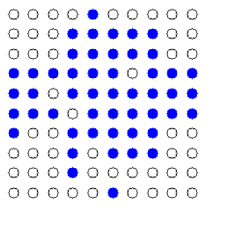
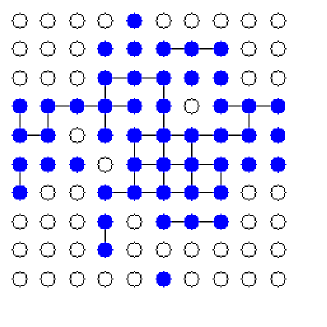
Figure 1: (a) Ising configuration at $T_{c}$: “down” spins are represented by filled circles. (b) Correct clusters are obtained from the configuration given in (a) by putting bonds between occupied sites with probability $p=1-e^{-2\beta J}$.

In the Ising model, for a given configuration of spins it is rather natural to define a cluster as a maximal set of $nn$ down parallel spins (Fig. 1). For some time these clusters were believed to be responsible for the correlations present in the Ising model. This idea was also based on numerical results which showed evidence that in two dimensions the mean cluster size diverges at the thermal critical point [5]. However the idea that the clusters could describe thermal correlations was definitively abandoned when it was shown, by numerical simulations in the three dimensional Ising model [46] and by exact solution on the Bethe lattice [47], that the percolation point appeared in the low density phase of down spins on the coexistence curve at a temperature $T_{p}$ before the critical point $T_{c}$ is reached ($T_{p}<T_{c}$).

Later it was suggested by topological arguments [48] that only in two dimensions the critical point coincides with the percolation point, but not necessarily in higher dimensions. The arguments followed two steps: in the first step it was argued that an infinite cluster of up spins is a necessary condition for having a spontaneous magnetization. This implies a percolation transition of down spins on the coexistence curve $T_{p}\leq T_{c}$, in the second step it was argued that due to topological reasons in two dimensions it is not possible to have an infinite cluster of up spins coexisting with an infinite cluster of down spins, which implies $T_{p}\geq T_{c}$. Combining with the previous inequalities one obtains in two dimensions $T_{p}=T_{c}$.

Later these results were proven rigorously [6, 7] along with many other results relating connectivity and thermodynamic quantities. For more details we refer to the original papers.

It is clear that the Ising clusters, defined as group of $nn$ parallel spins, do not have the property of describing correlated regions corresponding to spin fluctuations, as originally expected. In fact even in two dimensions, where the thermal critical point coincides with the percolation point, the Ising clusters were not suitable for such description. Series expansion showed that the mean cluster size diverges with an exponent, $\gamma^{*}=1.91{\pm}0.001$, rather different from the susceptibility exponent, $\gamma=1.75$ [8]. Later it has been shown exactly that $\gamma^{*}=91/48$ [49].

4.2 Ising Droplets

From the properties mentioned in Sect. 4.1, it appears that the Ising clusters are too big to describe the proper droplets. The reason is that there are two contributions to the Ising clusters. One is due to correlations but there is another contribution purely geometrical due to the fact that two $nn$ spins even in absence of correlation have a finite probability of being parallel. The last contribution becomes evident in the limit of infinite temperature and zero external field. In this case in fact, although there is no correlations and the susceptibility is zero, the cluster size is different from zero. In fact in $3d$ at infinite temperature there is even an infinite cluster of “up” and “down” spins.

Binder [5] proposed to cut the infinite cluster in order to have $T_{p}=T_{c}$ in $d=3$, but he did not give the microscopic prescription to do it. Later Coniglio and Klein [9] proposed to reduce the cluster size by introducing fictitious bonds between $nn$ parallel spins with probability $p_{b}$ (Fig. 1). These new clusters are made of $nn$ parallel spins connected by bonds. The original Ising cluster will either reduce its size or will break into smaller clusters. If $p_{b}=1$, we obtain the Ising clusters again. This case is known as the site correlated percolation problem because one looks at the properties of the Ising clusters just as in the random percolation problem. The main difference is that in random percolation the occupied sites are randomly distributed, while in this case the down (or up) spins are correlated according to the Ising Hamiltonian. In the infinite temperature limit one recovers random percolation. The case $p_{b}\neq 1$ is called site-bond correlated percolation [74].

A Hamiltonian formalism was proposed to study site correlated percolation [50]. This formalism was generalized in Ref. [9] to study site-bond correlated percolation. In this case for zero external field the Hamiltonian is given by the following dilute Ising $s-$state Potts Model (DIPM) :

$$-\mathcal{H}_{DP}=J_{b}\sum_{<ij>}(\delta_{\sigma_{i}\sigma_{j}}-1)(S_{i}S_{j}+1)+J\sum_{<ij>}S_{i}S_{j},$$ (31)

where $\sigma_{i}=1,\dots,s$ are Potts variables and the sum is over all nearest neighbor sites. In the same way as the s-state Potts model in the limit $s=1$ [51] describes the random bond percolation model, the DIPM describes percolation in the Ising model where the clusters are made of parallel spins connected by bonds with probability, $p_{b}=1-e^{-2\beta J_{b}}$.

In particular the average number of clusters $G$, that plays the role of the free energy in the percolation problem is given by $G=dF/ds|_{s=1}$, where

$$-\beta F=\lim_{N\rightarrow\infty}\frac{1}{N}\ln\left(\sum_{\{\sigma_{i}S_{i}\}}e^{-\beta\mathcal{H}_{DP}}\right).$$ (32)

At that time the DIPM was investigated in a different context by Berker et al [52]. The model exhibits the interesting properties that by choosing $J_{b}=J$ it coincides with a pure $s+1-$state Potts model. Therefore in the limit $s=1$ the DIPM coincides with the $s=2$ Potts model namely with the Ising model. Consequently $F$ becomes the Ising model free energy and $G$ has a singularity at the Ising critical point. This argument immediately suggested that the site-bond correlated percolation for $J_{b}=J$ namely with the bond probability given by

$$p_{b}\equiv p=1-e^{-2\beta J},$$ (33)

should reproduce the same critical behavior of the Ising model. Namely the percolation quantities become critical at the Ising critical point in the same way as the corresponding thermal quantities.

In fact using real space renormalization group arguments, it was possible to show that the size of the clusters of parallel spins connected by bonds with probability, $p_{b}$, given by Eq. (33), diverges at the Ising critical point with Ising exponents, exhibiting thus the same properties as the droplets in Fisher’s model. These clusters were called droplets to distinguish them from the Ising clusters.

4.3 Droplets in $2$ and $3$ dimensions

This site-bond correlated percolation problem has been studied by real space renormalization group in two dimensions [9, 96], by $\epsilon$ expansion, near six dimensions [56] and by Monte Carlo in two and three dimensions [45, 89, 92, 95, 83].

The renormalization group analysis shows that in $2d$ the Ising critical point is a percolation point for down or up spins connected by bonds for all values of bond probability such that $1\leq p_{b}<1-e^{-2\beta J}$. The fractal dimension $D^{*}=(\gamma^{*}/\nu+2)/2=187/96$ [49] being higher than the fractal dimension $D=(\gamma/\nu+2)/2=15/8$ for the value of $p_{b}\equiv p=1-e^{-2\beta J}$.

In the renormalization group language this means that there are two fixed points, one corresponding to the universality class of the Ising cluster, the other one corresponding to the droplets. In the first one the variable $J_{b}$ is irrelevant namely the scaling exponent associated to it, $y_{b}<0$. In the second fixed point associated to the droplets instead $y_{b}>0$. The result that the Ising critical point is a percolation point for a range of values of $p_{b}$, at the first sight seems counter-intuitive. In fact if the Ising critical point corresponds to the onset of percolation for Ising clusters ($p_{b}=1$), one would expect that for $p_{b}<1$ the clusters would not percolate anymore. The puzzle can be clarified by studying the fractal structure of the Ising clusters and the droplets at $T_{c}$ [43]. In fact it can be shown that $y_{b}$ is the scaling exponent of the red bonds, namely $L_{R}\sim l^{y_{b}}$ where $L_{R}$ is the number of red bonds between two connected sites separated by a distance of the order $l$, consequently the droplets, characterized by $y_{b}>0$, are made of links and blobs, like in random percolation. Due to the presence of links the cluster breaks apart and does not percolate anymore as the bond probability decreases. On the contrary the Ising clusters ($p_{b}=1$), characterized by $y_{b}<0$, are made only of blobs and no links, therefore by decreasing the bond probability the infinite cluster does not break and still percolates, until $p_{b}=p$.

In $3d$ at the Ising critical point, $T_{c}$, there is an analogous line of anomalous percolation point for clusters of down spins connected by bonds, for all values of bond probability such that $1\leq p_{b}<1-e^{-2\beta J}$, although the probability $P_{\infty}$ for a down spin to be in the infinite cluster is different from zero. More precisely the quantity $p_{ij}-P^{2}_{\infty}$ decays as a power law, where $p_{ij}$ is the probability that $i$ and $j$ are connected. For more details see Ref. [93]. As $p_{b}$ decreases towards $p=1-e^{-2\beta J}$ there is a crossover towards a different power law characterized by the Ising exponent, while $P_{\infty}$ goes to $0$.

4.4 Droplets in an external field

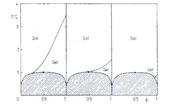
Figure 2: Montecarlo simulations of the $3d$ lattice gas model for three values of the bond probability $p_{b}=1-e^{-2c\beta J}$ with the constant $c=2.25,\,1,\,0.564$ from left to right. $\Phi$ is the density of down spins. The Gel and the Sol indicates the percolation and non percolation phase. From Ref. [57].

By keeping the same definition of droplets given above, in the case of an Ising model in an external field $H>0$ one finds a phase diagram in the $H,T$ plane or in the $M,T$ plane, with a percolation line of “down” spins ending at the Ising critical point (see Fig. 2). Along the percolation line one finds critical exponents in the universality class of random percolation with a cross-over to Ising critical exponents as the Ising critical point is approached [9]. In this context the Ising critical point is a higher order critical point for the percolation transition. This percolation line, also known as the Kertesz line, has received some attention [25, 58, 71, 72] (see for more details the review by Sator [2]). Although the Ising free energy has no singularity along this line some physical interpretation is given to the Kertesz line [67].

On the other hand this line disappears if the droplet definition is modified in the presence of an external field [12, 72], according to Kasteleyn and Fortuin formalism [59] and Swendsen and Wang approach [11]. In this approach the field is treated as a new interaction between each spin and a ghost site. Consequently for positive $H$ (negative $H$) an “up” (“down”) spin can be connected to the ghost spin with a probability $p_{H}=1-e^{-2\beta|H|}$. Droplets now are defined as a maximal set of spins connected by bonds where as before the bonds between nearest neighbor parallel spins have probability $p_{b}$ given by Eq. (33) and $p_{H}$ between spins and the ghost spin. Note that two far away spins can be easily connected through the ghost spin. In this way the presence of a positive (negative) magnetic field implies always the presence of an infinite cluster of “up” (“down”) spins.

4.5 Exact relations between connectivity and thermal properties

Interestingly it was also shown [12] that the droplets so defined with and without the external field have the same statistics of the clusters in the random cluster model introduced by Kasteleyn and Fortuin (KF) [59] (see Sect. 4.9), although the CK droplets and the KF clusters have a different meaning. Using the relations between the connectivity properties of the random cluster model and the thermal properties of the Ising model, it was finally possible to prove that in any dimension and for any temperature $T$ and external field $H\geq 0$, the following relations between connectivity and thermal properties hold [12]:

$$\left\{\begin{array}[]{l}\rho_{\infty}=m\\ {}{}\\ p_{ij}=g_{ij}\end{array}\right.$$ (34)

where $\rho_{\infty}$ is the density of up spins in the percolating droplet, $m$ is the magnetization per site, $p_{ij}$ is the probability that $i$ and $j$ are connected (through both finite or infinite droplet) and $g_{ij}=<S_{i}S_{j}>$.

In particular, for $T>T_{c}$ and zero external field $H\rightarrow 0$, we have that the magnetization $m=0$ and $g_{ij}$ coincides with the spin-spin pair correlation function. Consequently $\rho_{\infty}=0$, namely the probability for a spin to be in an infinite droplet is zero, and therefore $p_{ij}$ coincides with the probability that two spins $i$ and $j$ are in the same finite droplet. For $T<T_{c}$ instead we have $\rho_{\infty}=m>0$, and $p_{ij}=p^{f}_{ij}+p^{\infty}_{ij}$, where $p^{f}_{ij}$ ($p^{\infty}_{ij}$) is the probability that spins in $i$ and $j$ are in a finite (infinite) droplet. From Eq. (34) it follows for $T<T_{c}$:

$$p^{f}_{ij}+p^{\infty}_{ij}-\rho^{2}_{\infty}=<S_{i}S_{j}>-m^{2}.$$ (35)

By summing over $i$ and $j$ we have

$$S+(\Delta\rho_{\infty})^{2}=\chi,$$ (36)

where $S$ is the mean cluster size of the finite clusters, $(\Delta\rho_{\infty})^{2}$ is the fluctuation of the density of the infinite cluster and $\chi$ is the susceptibility. These exact results show that above $T_{c}$ mean cluster size and susceptibility coincide, while below $T_{c}$ there are two contributions to the susceptibility, one due to the mean cluster size and the second related to the fluctuation of the density of the infinity cluster. Monte Carlo calculations [89] show that both term have the same critical behavior as also occurs in random percolation [90, 91], so the mean cluster size $S$ diverges like the susceptibility. We expect that this is the case for dimensions up to $d=4$, the upper critical dimensionality of the Ising model. In mean field, as we will see, the mean cluster size below $T_{c}$ diverges with an exponent different from the susceptibility.

One very interesting application based on the KF approach was produced by Swendsen and Wang [11, 54], who elaborated a cluster dynamics which drastically reduced the slowing down near the critical point of the Ising and Potts model (see also [55] for further developments).

The droplet definition can be extended to the $nn$ antiferromagnetic Ising model [105] and to the Ising model with any ferromagnetic interaction $J_{ij}$ between sites $i$ and $j$ [92]. In this case the CK clusters are defined as set of parallel spins connected by bonds present between $i$ and $j$ with probability $p_{ij}=1-\exp{[-2\beta J_{ij}]}$. It can be shown that also in this case the relations (34) between connectivity and thermal quantities hold.

4.6 Ising Droplets above $d=4$

In Sect. 4.2 we have reported the relations Eq.s (34) and (35), which are exact and are valid in any dimension including mean field. As a matter of fact in mean field the percolation order parameter and the magnetization are identical and go to zero with the exponent $\beta=1/2$, while the mean cluster size above $T_{c}$ coincides with the susceptibility and diverges with the exponent $\gamma=1$. The same is true for the connectedness length above $T_{c}$, which coincides with the correlation length, and diverges with an exponent $\nu=1/2$. However below $T_{c}$ the mean cluster size diverges with an exponent $\gamma^{\prime}=1/2$ and the correlation length with an exponent $\nu^{\prime}=1/4$ [74, 12, 94]. This result is a consequence that the two terms in Eq. (35), the probability that two sites are in the same finite droplet, $p^{f}_{ij}$, and the correlation of the infinite droplet density at site $i$ and $j$, $p^{\infty}_{ij}-\rho^{2}_{\infty}$, do not scale in the same way, giving rise to two lengths, diverging respectively with exponents $\nu^{\prime}$ and $\nu$.

These somehow anomalous results are probably a consequence that the Ising model has an upper critical dimension $d_{c}=4$ while the DIPM which describes the droplet problem has an upper critical dimension $d_{c}=6$ [56]. In fact there are arguments that for $4\leq d\leq 6$ below $T_{c}$ the critical exponents are ${\displaystyle\nu^{\prime}=\frac{1}{d-2}}$, ${\displaystyle\gamma^{\prime}=\frac{2}{d-2}}$, $\beta=1/2$, $\eta=0$ and fractal dimension $D_{p}={\displaystyle\frac{1}{2}(d+2)}$, with an upper critical dimension $d_{c}=6$. Of course for $T>T_{c}$ the exponents are $\gamma=1$, $\nu=1/2$ and $\eta=0$.

Due to the breakdown of the mapping between thermal fluctuations and mean cluster size below $T_{c}$ above $d=4$, it is not possible to extend easily the geometrical picture, employed in random percolation, to explain the breakdown of hyperscaling in the Ising model. For a study of droplets inside the metastable region see Ref. [106].

4.7 Generalization to the $q$-state Potts Model

All the results found for the Ising case have been extended [10] to the $q$-state Potts model. This model is defined by the following Hamiltonian:

$$-{\cal H}_{q}=qJ\sum_{<ij>}\delta_{\sigma_{i}\sigma_{j}},$$ (37)

where the spin variables $\sigma_{i}$ can assume $q$ values, $\sigma_{i}=1,\dots,q$. This model coincides with the Ising model for $q=2$, reproduces the random percolation problem in the limit $q=1$ and the tree percolation model in the limit $q=0$ [51]. The geometrical approach developed in the previous sections for the Ising model, can be extended to the $q$-state Potts model. In particular one can define the site-bond Potts correlated percolation, where clusters are made of $nn$ spins in the same state, connected by bonds with bond probability $p_{b}$. By choosing $p_{b}=p=1-e^{-q\beta J}$, it is possible to show that these clusters percolate at the Potts critical temperature $T_{c}(q)$, with percolation exponents identical to the thermal exponents and therefore behave as the critical droplets.

The formalism is based on the following diluted Potts model [10, 97]:

$$-{\cal H}^{q}_{DP}=J_{b}\sum_{<ij>}(\delta_{\tau_{i}\tau_{j}}-1)\delta_{\sigma_{i}\sigma_{j}}+qJ\sum_{<ij>}\delta_{\sigma_{i}\sigma_{j}},$$ (38)

where the second term, which controls the distribution of spin variables, is the $q-$state Potts Hamiltonian, whereas the first term contains auxiliary Potts variables $\tau_{i}=1,2,\dots,s$ and controls the bonds distribution.

As in the Ising case, Hamiltonian (37) in the limit $s\rightarrow 1$ describes the site-bond Potts correlated percolation problem with $p_{b}$ given by $p_{b}=1-e^{-q\beta J_{b}}$. The droplets are obtained in the particular case $J_{b}=qJ$. For this value in fact Hamiltonian (37) for $s\rightarrow 1$ coincides with the $q$-state Potts model.

Once the Ising and Potts model has been mapped onto a percolation problem, we can extend some of the results of random percolation to thermal problems.

4.8 Fractal structure in the Potts Model: Links and blobs

Like in random percolation, also in the $q$-state Potts model it can be shown that at $T_{c}(q)$ the critical droplets have a fractal structure made of links and blobs, with a fractal dimension $D(q)=d-\beta(q)/\nu(q)$, where $\beta(q)$ and $\nu(q)$ are respectively the order parameter and correlation length exponent. Therefore $D(q)$ coincides with the magnetic scaling exponent $y_{H}(q)$. However the fractal dimension of the red bonds $D_{R}(q)$ does not coincide with the thermal scaling exponent $y_{T}(q)$, associated to the thermal variable $J$, like in random percolation. Instead $D_{R}(q)$ is found to coincide with the bond probability scaling exponent $y_{b}$ associated to the variable $J_{b}$ in Hamiltonian (37) [43].

Like for random percolation the fractal dimension of the red bonds coincides with the fractal dimension of the antired bonds. Using the mapping from the Potts model to the Coulomb gas [61], it is possible to obtain the exact value of the fractal dimension of the red bonds and of the external perimeter or hull [43]. For further exact results see also [62, 49].

Table 1: Fractal dimensions, for $d=2$, of the whole cluster ($D$), of the Hull ($D_{H}$), and of the red bonds ($D_{R}$) for the Potts droplets. It is also reported the thermal power exponent $y_{T}$.

$q$	$D$	$y_{T}$	$D_{H}$	$D_{R}$
$0$	$2$	$0$	$2$	$5/4$
$1$	$91/48$	$3/4$	$7/4$	$3/4$
$2$	$15/8$	$1$	$5/3$	$13/24$
$3$	$28/15$	$6/5$	$8/5$	$7/20$
$4$	$15/8$	$3/2$	$3/2$	$0$

From Table 1 it appears that the exact value of $D(q)$ does not vary substantially with $q$, for $d=2$. This observation can be understood by noting that, using this geometrical approach, the driving mechanism of the critical behavior can be viewed as coalescence of clusters just like in random percolation. Then one would expect for any $q$ that the fractal dimension should be close to the fractal dimension of the critical clusters in the percolation problem. This also explains the observation of Suzuky [60], known as strong universality, that for a large class of models the ratio $\gamma/\nu$ or $\beta/\nu$ do not vary appreciably. Since these ratios of critical exponents for fixed $d$ depend only on the magnetic scaling exponent, which is identical to the fractal dimension, the strong universality is consequence of the quasi-universal feature of the fractal dimension as discussed above. Unlikely the fractal dimension of the whole cluster, $D_{R}(q)$ and $D_{H}(q)$ do change substantially and characterize the different models as function of $q$. Particularly sensitive to $q$ is the fractal dimension of the red bonds, which has its largest value at $q=0$ (tree percolation), where the backbone is made only of links. As $q$ approaches $q_{c}$ the cluster becomes less ramified until the red bonds vanish ($D_{R}(4)=0$). This results in a drastic structural change from a links and blobs picture to a blobs picture only, anticipating a first order transition. Interestingly, the fractal dimension of the red bonds for $q=0$, $D_{R}=5/4$, has been related to the abelian sandpile model [84]. The reason why $D_{R}(q)$ is so model dependent is due to the fact that the fractal set of the red bonds is only a small subset of the entire droplet, and therefore this “detail” is strongly model dependent. Also the thermal exponent $y_{T}(q)$ is strongly model dependent, however so far it has not been found the geometrical characterization in terms of a fractal dimension for such exponent except $q=1$ (random percolation).

4.9 Fortuin Kasteleyn-Random Cluster Model

We will present here the random cluster model introduced by Kasteleyn and Fortuin. Let us consider the q-state Potts model on a $d-$dimensional hypercubic lattice. By freezing and deleting each interaction of the Hamiltonian (see Appendix), they managed to write the partition function of the Potts model, $Z=\sum_{\{\sigma_{i}\}}e^{-\beta{\cal H}_{q}}$, in the following way

$$Z=\sum_{C}p^{|C|}(1-p)^{|A|}q^{N_{C}}\,,$$ (39)

where $C$ is a configuration of bonds defined in the same hypercubic lattice, just like a bond configuration in the standard percolation model, $|C|$ and $|A|$ are respectively the number of bonds present and absent in the configuration $C$, and $N_{C}$ is the number of clusters in the configuration $C$.

In conclusion, in the KF formalism the partition function of the Potts model is identical to the partition function (39) of a correlated bond percolation model [59, 80] where the weight of each bond configuration $C$ is given by

$$W(C)=p^{|C|}(1-p)^{|A|}q^{N_{C}}$$ (40)

which coincides with the weight of the random percolation except for the extra factor $q^{N_{C}}$. They called this particular correlated bond percolation model, the random cluster model. Clearly for q = 1 the the cluster model coincides with the random percolation model.

Kasteleyn and Fortuin have related the percolation quantities associated to the random cluster model to the corresponding thermal quantities in the $q-$state Potts model [59]. In particular for the Ising case, $q=2$,

$$|\langle S_{i}\rangle|=\langle\gamma_{i}^{\infty}\rangle_{W}$$ (41)

and

$$\langle S_{i}S_{j}\rangle=\langle\gamma_{ij}\rangle_{W}\,,$$ (42)

where $\langle...\rangle$ is the Boltzmann average and $\langle...\rangle_{W}$ is the average over bond configurations in the bond correlated percolation with weights given by (40). Here $\gamma_{i}^{\infty}(C)$ is equal to 1 if the spin at $i$ belongs to the infinite cluster, $0$ otherwise; $\gamma_{ij}(C)$ is equal to 1 if the spins at sites $i$ and $j$ belong to the same cluster, $0$ otherwise.

Interestingly the connectivity properties in the KF random cluster model can be related to the CK droplets:

$$\rho_{\infty}=\langle\gamma_{i}^{\infty}\rangle_{W},$$ (43)

$$p_{ij}=\langle\gamma_{ij}\rangle_{W},$$ (44)

where $\rho_{\infty}$ and $p_{ij}$ are defined in Sect. 4.5. From Eq.s (41-44) it follows Eq.s (34).

5 Hill’s clusters

In this section we discuss the possibility to extend the definition of droplets to simple fluids. In 1955 Hill [63] introduced the concept of physical clusters in a fluid in an attempt to explain the phenomenon of condensation from a gas to a liquid. In a fluid made of particles interacting via a pair potential $u(r)$ physical clusters are defined as a group of particles pairwise bounded. A pair of particles is bounded if in the reference frame of their center of mass their total energy is less than zero. Namely their relative kinetic energy plus the potential energy is less than zero. The probability that two particles at distance $r$ are bounded can be calculated [63] and is given by

$$p_{\,\mbox{\tiny H}}(r)=\frac{4}{\pi}\int_{0}^{\sqrt{-\beta u(r)}}x^{2}e^{-x^{2}}\,dx\,.$$ (45)

More recently it was noted [64] that the bond probability Eq. (45) calculated for the interaction of the three dimensional $nn$ lattice gas model is almost coincident with the bond probability $p$ of Eq. (33). This implies that Hill’s physical clusters for the $3d$ lattice gas almost coincide with the droplets defined by Coniglio and Klein, and in fact Hill’s clusters percolate along a line almost indistinguishable from the droplets percolation line (see Fig. 2).

In order to calculate percolation quantities in a fluid in Ref. [65] the authors developed a theory based on Mayer’s expansion. In particular, using this theory they calculated analytically for a potential made of hard core plus an attractive interaction, the percolation line of Hill’s physical clusters in a crude mean field approximation and compared with the liquid gas coexistence curve. They found that the percolation line ended just below the critical point in the low density phase but not exactly at the critical point. For further developments of the theory see [66].

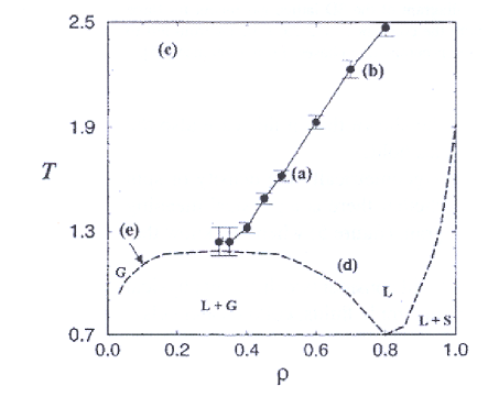
Figure 3: Phase diagram of the Lennard–Jones fluid using molecular dynamics. The full line corresponds to percolation of cluster following Hill’s definition. From Ref. [67].

Very recently, Campi et al. [67], using molecular dynamics have calculated the percolation line of Hill’s physical clusters for a Lennard–Jones potential. The results showed a percolation line ending close or at the critical point (Fig. 3) suggesting that Hill’s clusters are good candidates to describe the density fluctuations like the droplets in the lattice gas model, although there is no proof of relations analogous to those valid for the droplets in the lattice gas such as Eq. (34), which would prove that their size would diverge exactly at the critical point with thermal exponents.

Although Hill’s clusters may represent the critical fluctuation near the critical point, we may wonder whether they have a physical meaning away from the critical point. In particular we may wonder whether we can detect experimentally the percolation line in the phase diagram. In a Lennard–Jones fluid, molecular dynamics shows that quantities such as viscosity or diffusion coefficient do not seem to exhibit any anomalous behaviour through the percolation line [67]. In some colloids instead the percolation line is detected through a steep increase of the viscosity. What would be the difference in the two cases? The difference may rely in their lifetime. The possibility to detect the percolation line of these clusters is expected to depend on the lifetime of the clusters which in turn depends on the bond lifetime. The larger is the cluster lifetime the larger is the increase of the viscosity, the better the percolation line can be detected. In Sect. 7 we will discuss the behaviour of the viscosity as function of the lifetime of the clusters.

6 Clusters in weak and strong gels

In the previous section we have shown the case in which the probability of having a bond between two particles coincides with the probability that the two particles form a bound state defined according to Hill’s criterion. Now we want to show another mechanism leading to the formation of bound states, which is more appropriate to gels. The importance of connectivity in gels was first emphasized by Flory [68]. The application of percolation theory to gels was later suggested by de Gennes [69] and Stauffer [70, 73]. Here we consider a system made of monomers in a solvent. Following Ref. [74] we shall assume that the monomers can interact with each other in two ways. One is the usual van der Waals interaction, and the other is a directional interaction that leads to a chemical bond. A simple model for such a system is a lattice gas model where an occupied site represents a monomer and an empty site a solvent. For simplicity we can put equal to zero the monomer-solvent interaction and the solvent-solvent interaction, and include such interaction in an effective monomer-monomer interaction. The monomer-monomer interaction $\varepsilon_{ij}$ can reasonably be approximated by a nearest neighbour interaction

$$\varepsilon_{ij}=\left\{\begin{array}[]{c}-W\\ {}{}\hfil\\ -E\end{array}\right.$$ (46)

where $-W$ is the van der Waals type of attraction and $-E$ is the bonding energy. Of course, this second interaction, which is the chemical interaction, occurs only when the monomers are in particular configurations. For simplicity we can suppose that there is $1$ configuration which corresponds to the interaction of strength $E$, and $\Omega$ configurations which corresponds to the interaction of strength $W$. We expect $E\gg W$ and $\Omega\gg 1$. It can be easily calculated [74] that such a system is equivalent to a lattice gas model with an effective $nn$ interaction $-\varepsilon$ given by

$$e^{\beta\varepsilon}=e^{\beta E}+\Omega e^{\beta W}\,.$$ (47)

Therefore from the static point of view the system exhibits a coexistence curve and a critical temperature which characterizes the thermodynamics of the system. However the system microscopically behaves rather different from a standard lattice gas. In fact in a configuration in which two monomers are $nn$, in a standard lattice gas they feel one interaction, while in the system considered here with some probability $p_{b}$ they feel a strong chemical interaction $-E$ and with probability $1-p_{b}$ they feel a much smaller interaction $-W$. The probability $p_{b}$ can be easily calculated and is given by

$$p_{b}=\frac{e^{\beta E}}{e^{\beta E}+\Omega e^{\beta W}}\,.$$ (48)

In conclusion, the system from the static point of view is equivalent to a lattice gas with interaction $\varepsilon$ given by (47). However we can also study the percolation line of the clusters made by monomers connected by chemical bonds. This can be done by introducing bonds between $nn$ particles in the lattice gas with $nn$ interactions, the bonds being present with probability $p_{b}$ given by Eq. (48). By changing the solvent the effective interaction $W$ changes and one can realizes three cases topologically similar to those of Fig. 2, where the percolation line ends at the critical point or below the critical point in the low density or high density phase (for more details see [74]).

The lifetimes of the bonds are of the order of $e^{\beta E}$. Since $E$ is very large the lifetime could be very large. For an infinite bond lifetime the bonded clusters are permanent and the viscosity diverges due to the divergence of the mean cluster size (see for example [73]), and the percolation line can be easily detected. We consider three particular physical systems which could be rather emblematic of a general situation where the percolation line has been detected:

• Microemulsions of water in oil [85].

• Triblock copolymers in unicellar systems [86, 87].

• Gelatin water methanol systems [88].

In Fig.s 4, 5 and 6 we show respectively the phase diagram of the systems a), b), c), where it is shown the coexistence curve in the temperature-concentration diagram, together with “percolation lines”.

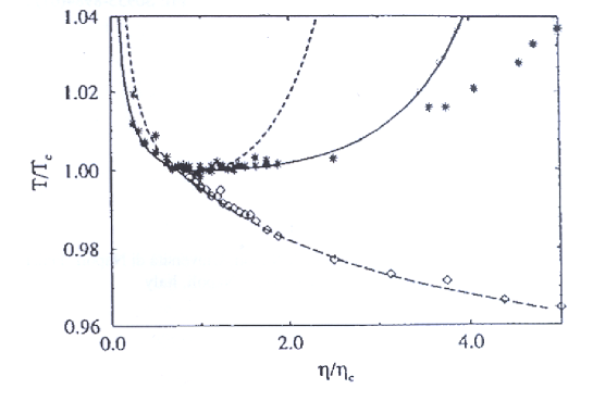
Figure 4: Experimental points in AOT/water/decane from Ref. [85] together with the coexistence curve and spinodal curve based on the Baxter’s model. The percolation line where the conductivity exhibits a steep increase has been fitted with the Baxter’s model.

In particular, in a) the system consists of three components AOT/water/decane. For the temperature and the concentration of interest, the system can be considered as made of small droplets of oil surrounded by water in a solvent. The droplets interact via a hard core potential plus short range attractive interaction. Because of the entropic nature of the attractive interaction, the coexistence curve is “upside-down” with the critical point being the minimum instead of the maximum (Fig. 4). The broken line is characterized by a steep increase of conductivity.

In b) the system is made of triblock copolymers unicellar in water solution, $c$ is the volume fraction of the unicelles (Fig. 5). The line is characterized by a steep increase in the viscosity.

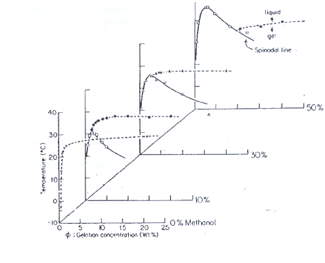
Figure 6: Sol-Gel transition temperature (solid symbols) and the spinodal temperature (open symbols) of gelatin-water-methanol mixtures as function of gelatin concentration. At the sol-gel transition the viscosity diverges. From Ref. [88].

In c) the system is made of gelatin dissolved in water + methanol; $\phi$ is the gelatin concentration. The broken lines are characterized by the divergence of the viscosity and correspond to the sol-gel transition. Each line represents a different value of the methanol concentration, which has been chosen in such a way that the line ends at the consolute point or, below it, in the low or high density phase (Fig. 6).

In all these experiments the consolute point is characterized by a thermodynamical singularity, where the correlation length and compressibility diverge. The other lines are usually ascribed to a “percolation” transition. However it is important to precise which are the relevant clusters in the three different systems. Also we would like to understand why, in system c), the viscosity diverges at the percolation transition, while in b) it reaches a plateau, and why in a) and b) the “percolation” lines end on the coexistence curve close to the critical point in the low density region . It is also important to realize that for each phenomenon is very important to define the proper cluster, which is responsible for the physical phenomenon. In the conductivity experiments in microemulsion the proper clusters are made of “touching” spheres similar to nearest neighbor particles in a lattice gas model. The viscoelastic properties of microemulsions may be more suitably described by clusters made of spheres pairwise bonded. For a more refined percolation model in microemulsion, see [53].

From the cluster properties of the lattice gas model we expect the infinite cluster is a necessary condition for a critical point therefore the percolation line ends just below the critical point in the low density region, as observed in the experiments described above and more recently in numerical simulations of models of interacting colloids [98].

In weak reversible gelatin the clusters are made of monomers (or polymers) bonded by strong interaction which leads to chemical bond. In this case the bond probability can be changed by changing the solvent and therefore the percolation line, by properly choosing the solvent, can end on the coexistence curve at or below the critical point.

The reason why the viscosity in the gel experiments diverges at the percolation point, while it reaches a plateau in colloids, is due to the lifetime of the bonds which is much longer in the first system than in the second [101, 99, 103]. In low density colloids the proper cluster to describe colloidal gelation also appear to be related to strong bonds with large bond lifetime [102, 100, 99]. When the relaxation time is much smaller than the bond lifetime the dynamics is dominated by the clusters, otherwise a crossover is expected towards a regime due to the crowding of the particles [102]. Percolation line of clusters pairwise bonded can also be defined in fluids, but due to the negligible lifetime cannot be detected.

7 Scaling behaviour of the viscosity

If the lifetime of the chemical bonds is infinite, the viscosity exhibits a divergence at the percolation threshold as recently shown in different models [75, 76, 78]

$$\eta\sim\xi^{\tilde{k}}\,,$$ (49)

where $\xi$ is the linear dimension of the critical cluster which diverges at the percolation threshold with the exponent $\nu$.

The relation between the diffusion coefficient $D(R)$ of a cluster of radius $R$ and the viscosity $\eta$ would be given by the Stokes–Einstein relation for a cluster radius much larger than $\xi$

$$D(R)\sim\frac{1}{R\eta}\,.$$ (50)

For cluster radius $R$  smaller than $\xi$ it has been proposed [79] that the viscosity will depend also on $R$ in such a way to satisfy a generalized Stokes–Einstein relation Eq. (50) with $\eta=\eta(R)$. When $R=\xi$ the viscosity $\eta(\xi)=\eta$, and from Eq. (50) one obtains the following scaling behaviour for $R$:

$$D(R)\sim R^{-(1+\tilde{k})}$$ (51)

therefore the relaxation time $\tau(R)$ for a cluster of radius $R$ is

$$\tau(R)\sim R^{1+\tilde{k}}\,.$$ (52)

If $\tau$ is the lifetime of a typical cluster, then a cluster of radius $R$ will contribute to the viscosity if $\tau(R)<\tau$, and therefore:

$$\eta\sim\xi^{\tilde{k}}f\left(\frac{\tau}{\xi^{1+\tilde{k}}}\right)\sim\left\{\begin{array}[]{ll}\xi^{\tilde{k}}{}{}{}{}{}&\tau>\xi^{1+\tilde{k}}\\ &\\ \tau^{\frac{\tilde{k}}{1+\tilde{k}}}&\tau<\xi^{1+\tilde{k}}\end{array}\right.$$ (53)

which implies that the viscosity will exhibit a steep increase followed by a plateau. The higher is $\tau$ the higher is the plateau.

The viscosity data on microemulsion (Fig. 5) shows in fact such a plateau, suggesting that the mechanism for the appearance of the plateau is linked to the bond lifetime which in turn is related to the cluster relaxation time.

8 Future Directions

In conclusion, we have discussed the interplay between percolation line and critical point in systems where thermal correlations play an important role. The problem to define the droplets in spin models is satisfactorily solved. However there are still some open problems. Above $d=4$ in the Ising model the definition of droplets presents some difficulties, probably related to the upper critical dimension for the percolation problem which is $6$. This type of difficulties does not allow for a trivial extensions of the arguments used in the random percolation problem, to explain the hyperscaling breakdown. Another open problem is the characterization of the thermal scaling exponent $1/\nu$, in terms of the fractal dimension of some subset of the critical droplet, as occurs in the random percolation problem.

In the last decade the KF,CK approach has been extended to frustrated systems. Interestingly this approach has led to a new frustrated percolation model, with unusual properties relevant to spin glasses and other glassy systems [104, 107]. However the precise definition of clusters, which are able to characterize the critical droplets for spin glasses, is still missing.

Although some advances have been obtained towards a droplet definition in Lennard Jones systems [67], a general definition for continuum models of fluids still needs to be formulated.

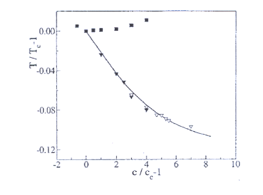
Figure 5: $L/64$ water system. Experimental points of the coexistence curve and percolation line, where the viscosity exhibits a steep increase. From Ref. [86].

Appendix A Random Cluster Model and Ising droplets

In 1969 Kasteleyn and Fortuin (KF) [59] introduced a correlated bond percolation model, called random cluster model, and showed that the partition function of this percolation model was identical to the partition function of $q-$state Potts model. They also showed that the thermal quantities in the Potts model could be expressed in terms of connectivity properties of the random cluster model. Much later in 1980 Coniglio and Klein [9] independently have used a different approach with the aim to define the proper droplets in the Ising model. It was only later that it was realized that the two approaches were related, although the meaning of the clusters in the two approaches is different. We will discuss these two approaches here, and show that their statistical properties are the same.

A.1 Random Cluster Model

Let us consider an Ising system of spins $S_{i}={\pm}1$ on a lattice with nearest-neighbour interactions and, when needed, let us assume periodic boundary conditions in both directions. All interactions have strength $J$ and the Hamiltonian is

$$\mathcal{H}(\{S_{i}\})=-\sum_{\langle i,j\rangle}J(S_{i}S_{j}-1)\,,$$ (54)

where $\{S_{i}\}$ represents a spin configuration and the sum is over $nn$ spins. The main point in the KF approach is to replace the original Ising Hamiltonian with an annealed diluted Hamiltonian

$$\mathcal{H}^{\prime}(\{S_{i}\})=-\sum_{<i,j>}J_{ij}^{\prime}(S_{i}S_{j}-1)\,,$$ (55)

where

$$J_{ij}^{\prime}=\left\{\begin{array}[]{ll}J^{\prime}&\mbox{with probability}~{}p\\ {}&{}\\ 0&\mbox{with probability}~{}(1-p)\ .\end{array}\right.$$ (56)

The parameter $p$ is chosen such that the Boltzmann factor associated to an Ising configuration of the original model coincides with the weight associated to a spin configuration of the diluted Ising model

$$e^{-\beta\mathcal{H}(\{S_{i}\})}\equiv\prod_{<i,j>}e^{\beta J(S_{i}S_{j}-1)}=\prod_{<i,j>}\left(pe^{\beta J^{\prime}(S_{i}S_{j}-1)}+(1-p)\right)\,,$$ (57)

where $\beta=1/k_{B}T$, $k_{B}$ is the Boltzmann constant and $T$ is the temperature. In order to satisfy (57) we must have

$$e^{\beta J(S_{i}S_{j}-1)}=pe^{\beta J^{\prime}(S_{i}S_{j}-1)}+(1-p)\ .$$ (58)

We take now the limit $J^{\prime}\mapsto\infty$. In such a case $e^{\beta J^{\prime}(S_{i}S_{j}-1)}$ equals the Kronecker delta $\delta_{S_{i}S_{j}}$ and from (58) $p$ is given by

$$p=1-e^{-2\beta J}.$$ (59)

From (57), by performing the products we can write

$$e^{-\beta\mathcal{H}(\{S_{i}\})}=\sum_{C}W_{KF}(\{S_{i}\},C)\,,$$ (60)

where

$$W_{KF}(\{S_{i}\},C)=p^{|C|}(1-p)^{|A|}\prod_{<i,j>\in C}\delta_{S_{i}S_{j}}\,.$$ (61)

Here $C$ is a configuration of interactions where $|C|$ is the number of interactions of strength $J^{\prime}=\infty$ and $|A|$ the number of interactions of strength $0$. $|C|+|A|=|E|$, where $|E|$ is the total number of edges in the lattice.

$W_{KF}(\{S_{i}\},C)$ is the statistical weight associated a) to a spin configuration $\{S_{i}\}$ and b) to a set of interactions in the diluted model where $|C|$ edges have $\infty$ strength interactions, while all the other edges have $0$ strength interactions. The Kronecker delta indicates that two spins connected by an $\infty$ strength interaction must be in the same state. Therefore the configuration $C$ can be decomposed in clusters of parallel spins connected by infinite strength interactions.

Finally the partition function of the Ising model $Z$ is obtained by summing the Boltzmann factor (60) over all the spin configurations. Since each cluster in the configuration $C$ gives a contribution of $2$, we obtain:

$$Z=\sum_{C}p^{|C|}(1-p)^{|A|}2^{N_{C}}\,,$$ (62)

where $N_{C}$ is the number of clusters in the configuration $C$.

In conclusion, in the KF formalism the partition function (62) is equivalent to the partition function of a correlated bond percolation model [59, 80] where the weight of each bond configuration $C$ is given by

$$W(C)=\sum_{\{S_{i}\}}W_{KF}(\{S_{i}\},C)=p^{|C|}(1-p)^{|A|}2^{N_{C}}$$ (63)

which coincides with the weight of the random percolation except for the extra factor $2^{N_{C}}$. Clearly all percolation quantities in this correlated bond model weighted according to Eq. (63) coincide with the corresponding percolation quantities of the KF clusters made of parallel spins connected by $\infty$ strength interaction, whose statistical weight is given by (61). Moreover using (61) and (60) Kasteleyn and Fortuin have proved that [59]

$$|\langle S_{i}\rangle|=\langle\gamma_{i}^{\infty}\rangle_{W}$$ (64)

and

$$\langle S_{i}S_{j}\rangle=\langle\gamma_{ij}\rangle_{W}\,,$$ (65)

where $\langle...\rangle$ is the Boltzmann average and $\langle...\rangle_{W}$ is the average over bond configurations in the bond correlated percolation with weights given by (63). Here $\gamma_{i}^{\infty}(C)$ is equal to 1 if the spin at site $i$ belongs to the spanning cluster, $0$ otherwise; $\gamma_{ij}(C)$ is equal to 1 if the spins at sites $i$ and $j$ belong to the same cluster, $0$ otherwise.

A.2 Connection between the Ising droplets and the Random Cluster Model

In the approach followed by Coniglio and Klein [9], given a configuration of spins, one introduces at random connecting bonds between $nn$ parallel spins with probability $p_{b}$, antiparallel spins are not connected with probability $1$. Clusters are defined as maximal sets of parallel spins connected by bonds. The bonds here are fictitious, they are introduced only to define the clusters and do not modify the interaction energy as in the FK approach. For a given realization of bonds we distinguish the subsets $C$ and $B$ of $nn$ parallel spins respectively connected and not connected by bonds and the subset $D$ of $nn$ antiparallel spins. The union of $C$, $B$ and $D$ coincides with the total set of $nn$ pair of spins $E$. The statistical weight of a configuration of spins and bonds is [81, 12]

$$W_{CK}(\{S_{i}\},C)=p_{b}^{\mid C\mid}(1-p_{b})^{\mid B\mid}e^{-\beta\mathcal{H}(\{S_{i}\})}\,,$$ (66)

where $|C|$ and $|B|$ are the number of $nn$ pairs of parallel spins respectively in the subset $C$ and $B$ not connected by bonds.

For a given spin configuration, using Newton binomial rule, we have the following sum rule

$$\sum_{C}p_{b}^{\mid C\mid}(1-p_{b})^{\mid B\mid}=1.$$ (67)

From Eq. (67) follows that the Ising partition function, $Z$, may be obtained by summing (66) over all bond configurations and then over all spin configurations.

$$Z=\sum_{\{S_{i}\}}\sum_{C}W_{CK}(\{S_{i}\},C)=\sum_{\{S_{i}\}}e^{-\beta\mathcal{H}(\{S_{i}\})}\ .$$ (68)

The partition function of course does not depend on the value of $p_{b}$ which controls the bond density. By tuning $p_{b}$ instead it is possible to tune the size of the clusters. For example by taking $p_{b}=1$ the clusters would coincide with nearest neighbour parallel spins, while for $p_{b}=0$ the clusters are reduced to single spins. By choosing the droplet bond probability $p_{b}=1-e^{-2\beta J}\equiv p$ and observing that $e^{-\beta\mathcal{H}(\{S_{i}\})}=e^{-2\beta J|D|}$, where $|D|$ is the number of antiparallel pairs of spins, the weight (66) simplifies and becomes:

$$W_{CK}(\{S_{i}\},C)=p^{\mid C\mid}(1-p)^{\mid A\mid}\,,$$ (69)

where $|A|=|B|+|D|=|E|-|C|$.

From (69) we can calculate the weight $W(C)$ that a given configuration of connecting bonds $C$ between $nn$ parallel spins occurs. This configuration $C$ can occur in many spin configurations. So we have to sum over all spin configurations compatible with the bond configuration $C$, namely

$$W(C)=\sum_{\{S_{i}\}}W_{CK}(\{S_{i}\},C)\prod_{<i,j>\in C}\delta_{S_{i}S_{j}}\,,$$ (70)

where, due to the product of the Kronecker delta, the sum is over all spin configurations compatible with the bond configuration $C$. From (69) and (70) we have

$$W(C)=\sum_{\{S_{i}\}}p^{\mid C\mid}(1-p)^{\mid A\mid}\prod_{<i,j>\in C}\delta_{S_{i}S_{j}}=p^{|C|}(1-p)^{|A|}2^{N_{C}}\,.$$ (71)

Consequently in (68) by taking first the sum over all spins compatible with the configuration $C$, the partition function $Z$ can be written as in the KF formalism (62).

$$Z=\sum_{C}p^{|C|}(1-p)^{|A|}2^{N_{C}}.$$ (72)

In spite of the strong analogies the CK clusters and the KF clusters have a different meaning. In the CK formalism the clusters are defined directly in a given configuration of the Ising model as parallel spin connected by fictitious bonds, while in the KF formalism clusters are defined in the equivalent random cluster model. However, due to the equality of the weights (69) and (61) the statistical properties of both clusters are identical [12] and due to the relations between (61) and (63) both coincide with those of the correlated bond percolation whose weight is given by (63). More precisely, any percolation quantity $g(C)$ which depends only on the bond configuration has the same average

$$\langle g(C)\rangle_{KF}=\langle g(C)\rangle_{CK}=\langle g(C)\rangle_{W}\,,$$ (73)

where $\langle...\rangle_{KF}$, $\langle...\rangle_{CK}$ are the average over spin and bond configurations with weights given by (61) and (69) respectively and $\langle...\rangle_{W}$ is the average over bond configurations in the bond correlated percolation with weights given by (63). In view of (73) it follows [12]

$$|\langle S_{i}\rangle|=\langle\gamma_{i}^{\infty}\rangle_{CK}$$ (74)

and

$$\langle S_{i}S_{j}\rangle=\langle\gamma_{ij}\rangle_{CK}\,.$$ (75)

We end this section noting that in order to generate an equilibrium CK droplet configuration in a computer simulation, it is enough to equilibrate a spin configuration of the Ising model and then introduce at random fictitious bonds between parallel spins with a probability given by (59).

• Primary Literature

• Books and Reviews

• Grimmett GR (1989) Percolation. Springer, Berlin

• Sahimi M (1994) Application of Percolation Theory. Taylor and Francis

References

- [1] Mayer J E (1937) J. Chem. Phys. 5: 67; Mayer J E and Ackermann P G (1937) J. Chem. Phys. 5: 74; Mayer J E and Harrison S F (1938) J. Chem. Phys. 6: 87; Mayer J E and Mayer M G (1940) Statistical Mechanics. Wiley, New York/Toronto.
- [2] Sator N (2003) Physics Reports 376: 1
- [3] Fisher M E (1967) Physics (N.Y.) 3: 255; Fisher M E (1967) J. Appl. Phys. 38: 981; Fisher M E and Widom B (1969) J. Chem. Phys. 50: 3756. Fisher M E (1971). In: Critical Phenomena, Proceedings of the International School of Physics “Enrico Fermi” Course LI, Varenna on lake Como (Italy), Green M S (ed), Academic, New York, p. 1.
- [4] Frenkel J (1939) J. Chem. Phys. 7:200; Frenkel J (1939) J. Chem. Phys. 7:538.
- [5] Binder K (1976) Ann. Phys. (NY) 98:390.
- [6] Coniglio A, Nappi C, Peruggi F and Russo L(1976) Comm. Math. Phys. 51: 315
- [7] Coniglio A, Nappi C, Peruggi F and Russo L (1977) J. Phys. A 10: 205
- [8] Sykes M F and Gaunt D S (1976) J. Phys. A 9: 2131.
- [9] Coniglio A and Klein W (1980) J. Phys. A 13: 2775;
- [10] Coniglio A and Peruggi F (1982) J. Phys. A 15: 1873
- [11] Swendsen R H and Wang J S (1987) Phys. Rev. Lett. 58: 86
- [12] Coniglio A, di Liberto F, Monroy G and Peruggi F (1989) J. Phys. A 22: L837
- [13] Mandelbrot BB (1982) The fractal geometry of nature. Freeman, San Francisco
- [14] A. Coniglio (1985) Finely Divided Matter. In: Proc. les Houches Winter Conference, Boccara N and Daoud M (ed), Springer Verlag, New York
- [15] Weinrib A (1984) Phys. Rev. B 29: 387; Weinrib A and Halperin B I (1983) Phys. Rev. B 27: 413; Sahimi M, Knackstedt M A and Sheppard A P (2000) Phys. Rev. E 61: 4920; Sahimi M and Mukhopadhyay (1996) Phys. Rev. E 54: 3870; Makse H A, Havlin S, Schwartz M and Stanley H E (1996) Phys. Rev. E 53: 5445
- [16] Ma Y G (1999) Phys. Rev. Lett. 83:3617;Ma Y G, Han D D, Shen W Q, Cai X Z, Chen J G, He Z J Long J L, Ma G L, Wang K, Wei Y B, Yu L P, Zhang H Y, Zhong C, Zhou X F and Zhu Z Y (2004) J. Phys. G: Nucl. Part. Phys. 30: 13
- [17] Fortunato S, Satz H (2000) Nuclear Physics B, Proceedings Supplements 83: 452
- [18] Bialas P, Blanchard P, Fortunato S, Gandolfo D and Satz H (2000) Nuclear Physics B 583: 368; Blanchard P, Digal S, Fortunato S, Gandolfo D, Mendes T and Satz H (2000) J. Phys. A: Math. Gen. 33: 8603
- [19] Campi X and Krivine H (2005) Phys. Rev. C 72: 057602; Campi X, Krivine H, Plagnol E, Sator N (2003) Phys. Rev. C 67: 044610; Mader C M, Chappars A, Elliott J B, Moretto L G,, Phair L, Wozniak G J (2003) Phys. Rev. C 68: 064601
- [20] Makse H A, Havlin S and Stanley H E (1995) Nature 377: 608; Makse H A, Andrade J S Jr, Batty M, Havlin S and Stanley H E (1998) Phys. Rev. E 58: 7054
- [21] Bastiaansen P J M and Knops H J F (1997) J. Phys. A: Math. Gen. 30: 1791
- [22] Bug A L R, Safran S A, Grest G S, Webman I (1985) Phys. Rev. Lett. 55: 1896; Safran S A, Webman I, Grest G S (1985) Phys. Rev. A 32: 506
- [23] Abete T, de Candia A, Lairez D, Coniglio A (2004) Phys. Rev. Lett. 93: 228301
- [24] Essam J W (1980) Rep. Prog. Phys. 43: 833
- [25] Stauffer D and Aharony A (1994) Introduction to Percolation Theory. Taylor and Francis.
- [26] Bunde A and Havlin S (1991) Percolation I. In: Fractals and Disordered Systems, Bunde A and Havlin S (ed), Springer Verlag, New York, pp. 51 - 95; Havlin S, Bunde A Percolation II. In: Fractals and Disordered Systems, Bunde A and Havlin S (ed), Springer Verlag, New York, pp. 97 - 149.
- [27] de Arcangelis L (1987) J. Phys. A 20: 3057
- [28] Kirkpatrick S (1978) AIP Conference Proc. 40:99
- [29] Fortunato S, Aharony A, Coniglio C and Stauffer D (2004) Phys. Rev. E 70: 056116
- [30] Aizenman M (1997) Nuclear Physics B 485: 551.
- [31] Hu CK and Lin CY (1996) Phys. Rev. Lett. 77: 8
- [32] for a minireview on the multiplicity of the infinite clusters, see Stauffer D (1997) Physica A 242: 1
- [33] Skal A S and Shklovskii B I (1975) Sov. Phys. Semicond. 8: 1029
- [34] de Gennes P G (1976) La Recherche 7: 919
- [35] Stanley H E (1977) J. Phys. A 10: l211 (1977)
- [36] Aharony A, Gefen Y and Kapitulnik A (1984) J. Phys. A 17: l197; Alexander S, Grest G S, Nakanishi H and Witten T A (1984) J. Phys. A 17: L185
- [37] Birgeneau R J, Cowley R A Shirane G, Tarvin J A and Guggenheim H J (1976) Phys. Rev. Lett. 37: 940. Birgeneau R J, Cowley R A Shirane G and Guggenheim H J (1980) Phys. Rev. B 21: 317
- [38] Gefen Y, Aharony A, Mandelbrot B B and Kirkpatrick S (1981) Phys. Rev. Lett. 47: 1771
- [39] Coniglio A (1981) Phys. Rev. Lett. 46: 250
- [40] Coniglio A (1982) J. Phys. A 15: 3829
- [41] Pike R and Stanley H E (1981) J. Phys. A 14: L169
- [42] Coniglio A (1983). In: Proceedings of Erice School on Ferromagnetic Transitions, Springer Verlag, New York
- [43] Coniglio A (1989) Phys. Rev. Lett. 62: 3054
- [44] Coniglio A and Stanley H E (1984) Phys. Rev. Lett. 52: 1068
- [45] Stauffer D (1981) J. Phys. Lett. 42: L49
- [46] Muller–Krhumbaar H (1974) Phys. Lett. A 50: 27
- [47] Coniglio A (1976) Phys. Rev. B 13: 2194
- [48] Coniglio A (1975) J. Phys. A 8: 1773
- [49] Stella A L and Vanderzande C (1989) Phys. Rev. Lett. 62: 1067
- [50] Murata KK (1979) J. Phys. A 12: 81
- [51] Wu F (1982) Rev. Mod. Phys. 54: 235
- [52] Nienhuis B, Berker A N, Riedel E K and Shick M (1979) Phys. Rev. Lett. 43:737
- [53] Grest GS, Webman I, Safran SA, and Bug ALR (1986) Phys. Rev. A 33: 2842
- [54] Wang J S and Swendsen R (1990) Physica A 167: 565
- [55] Wolff U (1988) Phys. Rev. Lett. 60: 1461; Wolff U (1989) Phys. Lett. B 228: 379; Wolff U (1989) Phys. Rev. Lett. 62: 361.
- [56] Coniglio A and Lubensky T (1980) J. Phys. A 13: 1783
- [57] Kertesz J, Coniglio A and Stauffer D (1983) Clusters for random and interacting percolation. In: Percolation structures and processes, Annals of the Israel Physical Society 5, Deutscher G, Zallen R and Adler J (ed), Adam Hilger (Bristol) and The Israel Physical Physical Society (Jerusalem), pp. 121 -147
- [58] Kertesz J (1989) Physica A 161: 58
- [59] Kasteleyn P W and Fortuin C M (1969) J. Phys. Soc. Japan Suppl. 26: 11; Fortuin C M and Kasteleyn P W (1972) Physica 57: 536
- [60] Suzuki M (1974) Progr. Theor. Physics (Kyoto) 51: 1992
- [61] Saleur H and Duplantier B (1987) Phys. Rev. Lett. 58: 2325; Duplantier B and Saleur H (1989) Phys. Rev. Lett. 63: 2536
- [62] Blote H W J, Knops Y M M, Nienhuis B (1992) Phys. Rev. Lett. 68: 3440
- [63] Hill T L (1955) J. Chem. Phys. 23: 617
- [64] Campi X, Krivine H and Puente A (1999) Physica A 262: 328
- [65] Coniglio A, De Angelis U, Forlani A and Lauro G (1977) J. Phys. A: Math. Gen. 10: 219; and Coniglio A, De Angelis U and Forlani A (1977) J. Phys. A: Math. Gen. 10: 1123
- [66] Given JA and Stell G (1991) J. Phys. A: Math. Gen. 24: 3369
- [67] Campi X, Krivine H and Sator N (2001) Physica A 296: 24
- [68] Flory P J (1941) J. Am. Chem. Soc. 63: 3083; see also the classic book: Flory P J (1979) Principles of Polymer Chemistry. Cornell University Press. Ithaca
- [69] de Gennes P G (1975) J. Phys (Paris) 36: 1049; see also: de Gennes P G (1979) Scaling concepts in polymer physics (Ithaca: Cornell University Press)
- [70] Stauffer D (1976) J. Chem. Soc. Faraday Trans. 72: 1354
- [71] Stauffer D (1990) Physica A 168: 614
- [72] Wang JS (1989) Physica A 161:249
- [73] For a review on percolation and gelation, see: Stauffer D, Coniglio A and Adam M (1982) Polymer Networks 44: 103
- [74] Coniglio A, Stanley H E and Klein W (1979) Phys. Rev. Lett. 42: 518; Coniglio A, Stanley H E and Klein W (1982) Phys. Rev. B 25: 6805
- [75] Del Gado E, de Arcangelis L and Coniglio A (2000) Eur. Phys. J. E 2: 359
- [76] Broderix K, Löwe H, Müller P and Zippelius A (2000) Phys. Rev. E 63: 011510
- [77] See also Dunn A G, Essam J W, Ritchie D S (1975) J. Phys. C 8: 4219; Cox M A A and Essam J W (1976) J. Phys C 9: 3985
- [78] Vernon D C, Plischke M, Joos B (2001) Phys. Rev. E 64: 031505
- [79] Martin J E, Adolf D and Wilcoxon J P (1988) Phys. Rev. Lett. 61: 2620
- [80] Hu CK (1984) Phys. Rev. B 29: 5103; Hu CK (1992) Phys. Rev. Lett. 69: 2739; Hu CK, Mak KS (1989) Phys. Rev. B 40: 5007;
- [81] Coniglio A (1990). In: Correlation and connectivity - Geometric aspects of Physics, Chemistry and Biology, Stanley H E and Ostrowsky W (ed), NATO ASI series, vol. 188
- [82] Harris A B, Lubensky T C, Holcomb W and Dasgupta C (1975) Phys. Rev. Lett. 35: 327
- [83] Heermann D W and Stauffer D (1981) Z. Phys. B 44: 339
- [84] Dhar D (1999) Physica A 263: 4
- [85] Chen S H, Rouch J, Sciortino F and Tartaglia P (1994) J. Phys. Cond. Matter 6: 10855
- [86] Mallamace F, Gambadauro P, Micali N, Tartaglia P, Liao C and Chen S H (2000) Phys. Rev. Lett. 84: 5431
- [87] Mallamace F, Chen S H, Liu Y, Lobry L and Micali N (1999) Physica A 266: 123
- [88] Tanaka T, Swislow G and Ohmine I (1979) Phys. Rev. Lett. 42: 1556
- [89] Roussenq J, Coniglio A and Stauffer D (1982) J. Phys. (Paris) 43: L703
- [90] Coniglio A and Stauffer D (1980) Lett. Nuovo Cimento 28: 33
- [91] Chayes J T, Chayes L, Grimmet G R, Kesten H and Schonmann R (1989) Ann. Probab. 17: 1277
- [92] Jan N, Coniglio A and Stauffer D (1982) J. Phys. A 15: L699
- [93] Coniglio A and Figari R (1983) J. Phys. A: Math. Gen. 16: L535
- [94] Chayes L, Coniglio A, Machta J, Shtengel K (1999) J. Stat. Phys. 94: 53
- [95] Odagaki T, Ogita N and Matsuda H (1975) J. Phys. Soc. Japan 39: 618
- [96] Coniglio A and Zia R V P (1982) J. Phys. A: Math. Gen. 15: L399
- [97] Temesvari T (1984) J. Phys A: Math. Gen. 17: 1703; Janke W, Schakel A M J (2004) Nucl. Phys. B 700: 385; Qian X, Deng Y, Blote H W J (2005) Phys. Rev. E 72: 056132; Deng Y, Guo W, Blote H W J (2005) Phys. Rev. E 72: 016101; Balog I and Uzelac K (2007) Phys. Rev. E 76: 011103
- [98] Romano F, Tartaglia P, and Sciortino F (2007) J. Phys.: Condens. Matter 19: 322101; Zaccarelli E (2007) J. Phys.: Condens. Matter 19: 323101
- [99] Saika-Voivod I, Zaccarelli E, Sciortino F, Buldyrev S V, and Tartaglia P (2004) Phys. Rev. E 70: 041401
- [100] Campbell A I, Anderson V J, van Duijneveldt J S, and Bartlett P (2005) Phys. Rev. Lett. 94: 208301
- [101] Del Gado E, Fierro A, de Arcangelis L, and Coniglio A (2004) Phys. Rev. E 69: 051103
- [102] Coniglio A, Abete T, de Candia A, Del Gado E, and Fierro A, (2007) J. Phys.: Condens. Matter 19: 205103; de Candia A, Del Gado E, Fierro A, Sator N, and Coniglio A (2005) Physica A 358: 239; Coniglio A, de Arcangelis L, Del Gado E, Fierro A and Sator N (2004) J. Phys.: Condens. Matter 16: S4831; Gimel JC, Nicolai T and Durand D (2001) European Physical Journal E 5:415
- [103] Mallamace F, Chen S H, Coniglio A, de Arcangelis L, Del Gado E, and Fierro A (2006) Phys. Rev. E 73: 020402
- [104] Coniglio A, di Liberto F, Monroy G, Peruggi F (1991) Phys. Rev. B 44:12605; Coniglio A (2000) Physica A 281: 129
- [105] Amitrano C, di Liberto F, Figari R and peruggi F (1983) J. Phys. A: Math. Gen. 16: 3925
- [106] Klein W, Gould H, Tobochnik J, Alexander FJ, Anghel M, and Johnson G (2000) Phys. Rev. Lett. 85:1270; Padoa Schioppa C, Sciortino F, Tartaglia P (1998) Phys. Rev. E 57: 3797; Heerman DW, Coniglio A, Klein W, Stauffer D (1984) J. Stat. Phys. 36:447
- [107] Machta J, Newman CM, Stein DL (2007) J. Stat. Phys. 130: 113
-