Single-photon scattering with counter rotating wave interaction

Abstract

Recent experiments have pushed the studies on atom-photon interactions to the ultrastrong regime, which motivates the exploration of physics beyond the rotation wave approximation. Here we study the single-photon scattering on a system composed by a coupling cavity array with a two-level atom in the center cavity, which, by varying two outside coupling parameters, corresponds to a model from a supercavity QED to a waveguide QED with counter-rotating wave (CRW) interaction. By applying a time-independent scattering theory based on the bound states in the scattering region, we find that the CRW interaction obviously changes the transmission valley even in the weak atom-cavity coupling regime; In particular, the CRW interaction leads to an inelastic scattering process and a Fano-type resonance, which is directly observed in the crossover from the supercavity QED case to the waveguide QED case. Predictably, our findings provide the potential of manipulating the CRW effects in realistic systems.

I Introduction

Recent experiments on diverse systems, such as circuit QEDs Niemczyk et al. (2010); Forn-Díaz et al. (2010); Baust et al. (2016), 2d electron gases Scalari et al. (2012), spiropyran molecules Schwartz et al. (2011), and semiconductor quantum wells Geiser et al. (2012), have pushed the research on photon-atom interactions to the ultrastrong regime, where the coupling is so strong that the rotating wave approximation (RWA) Jaynes and Cummings (1963) is not valid any longer, and the effects from the counter rotating wave interaction (CRW) can not be neglected.

In the RWA, the interacting photon and atom only exchange their excitations, thus the total excitation is conserved, which greatly simplifies the underlying physics and the theoretical treatments. The CRW interaction makes the total excitation not conserved, which makes the relative phenomena and the calculations become complex. To solve the calculation problem, several theoretical methods are introduced, such as, the generalized rotating-wave approximation (GRWA) Irish (2007), the analytical solution in the Bargmann space Braak (2011), and the numerical method based on matrix product states (MPS) Verstraete et al. (2008); García-Ripoll (2006).

To study the effects from the CRW interaction, it is convenient to investigate the single-photon scattering with an (artificial) atom in a one dimensional supercavity (SC) or waveguide Shen and Fan (2005). In the RWA, a one dimensional waveguide model is composed of coupling cavity array (CCA) with one cavity locating a two-level atom is firstly proposed in Ref. Zhou et al. (2008). An extension to present a SC-QED model is given in Ref. Zhu et al. (2014), where the concept of SC is borrowed from Ref. Gong et al. (2008). A natural problem is to extend the above models to the ultrastrong coupling regime. In fact, the CCA waveguide model including the CRW interaction is firstly studied in Ref. Wang et al. (2012) by using the GRWA. Then a remarkable result from this model in Ref. Sanchez-Burillo et al. (2014) is to discover an inelastic scattering process by using wave packet scattering simulation based on MPS algorithm.

In this article, we extend the SC-QED model to the ultrastrong regime, and apply the time-independent scattering theory to study the single photon transmission spectrum. Further more, our method is a unified frame to study the crossover from the SC-QED model to the waveguide QED model. In particular, we will show how the CRW interaction affect the single photon transmission in our model. For example, we find that there is an obvious effect in the photon transmission even in the weak coupling regime; the inelastic scattering also occurs in the SC-QED model as that predicted in the waveguide QED model Sanchez-Burillo et al. (2014).

The rest of this paper is built up as follows. In Sec. II, we introduce our model and numerically calculate the bound states of the SC, which is further confirmed by the Brillouin-Wigner perturbation theory Hubač and Wilson (2010). Based on the single-photon scattering mechanism given in Sec. II.2, the numerical results of the single-photon scattering process in our model are presented in Sec. III, showing how the CRW interaction affects the single photon transmission. In Sec. IV, we give some discussions and draw the conclusions.

II Model And Basic Scattering Processes

II.1 The model and Hamiltonian

As shown in Fig. 1, the system we consider contains a one-dimensional coupled cavity array (CCA) with infinite length and a two-level atom, where each cavity is represented by an empty circle and the two-level atom is represented by a red solid circle. The cavities in the CCA are labeled by integers in increasing order from left to right. The photonic hopping strengths between the neighbouring cavities $l$ and $l+1$ are $\eta$ for $l=0$ or $l=N$ and $\xi$ for others. When $\eta\ll\xi$, the CCA between $l=1$ and $l=N$ forms a multi-mode cavity, which will be named as a SC. The two-level atom that locates in the $s$-th cavity of the SC (Let $N$ be odd, $s\equiv\frac{N+1}{2}$), together with the SC, constructs a cavity-QED system, denoted as the SC system in Fig. 1.

Figure 1: (Color online). Demonstration of our model. A single photon (blue right arrow) with the momentum $\vec{k}_{0}$ injects from the left end of the 1D infinite CCA and the transmission spectrum is measured on the right side.

The Hamiltonian of our system is written as (we set $\hbar=1$)

$$\hat{H}=\hat{H}_{S}+\hat{H}_{L}+\hat{H}_{R}+\hat{H}_{LS}+\hat{H}_{SR},$$ (1)

where

$$\hat{H}_{S} = \omega_{c}\sum^{N}_{j=1}\hat{a}^{\dagger}_{j}\hat{a}_{j}-\xi\sum^{N}_{j=2}(\hat{a}^{\dagger}_{j}\hat{a}_{j-1}+h.c.)+\frac{\omega_{a}}{2}\hat{\sigma}_{z}$$ (2a)

$$\quad{}+g\hat{\sigma}_{x}(\hat{a}^{\dagger}_{s}+\hat{a}_{s}),$$

$$\hat{H}_{L} = \sum^{0}_{j=-\infty}[\omega_{c}\hat{a}^{\dagger}_{j}\hat{a}_{j}-\xi(\hat{a}^{\dagger}_{j}\hat{a}_{j-1}+\hat{a}^{\dagger}_{j-1}\hat{a}_{j})],$$ (2b)

$$\hat{H}_{R} = \sum^{\infty}_{j=N+1}[\omega_{c}\hat{a}^{\dagger}_{j}\hat{a}_{j}-\xi(\hat{a}^{\dagger}_{j}\hat{a}_{j+1}+\hat{a}^{\dagger}_{j+1}\hat{a}_{j})],$$ (2c)

$$\hat{H}_{LS} = -\eta(\hat{a}^{\dagger}_{0}\hat{a}_{1}+\hat{a}^{\dagger}_{1}\hat{a}_{0}),$$ (2d)

$$\hat{H}_{SR} = -\eta(\hat{a}^{\dagger}_{N}\hat{a}_{N+1}+\hat{a}^{\dagger}_{N+1}\hat{a}_{N}).$$ (2e)

Here $\hat{H}_{S}$ is the Hamiltonian of the SC system, $\hat{H}_{L}$ ($\hat{H}_{R}$) describes the left (right) channel which is used to input (output) photons, and $\hat{H}_{LS}$ ($\hat{H}_{SR}$) describes the interaction between the SC system with the left (right) channel. The operator $\hat{a}^{\dagger}_{j}$ ($\hat{a}_{j}$) is the photon creation (annihilation) operator for the $j$-th cavity, $\hat{\sigma}_{-}=|g\rangle\langle e|$ ($\hat{\sigma}_{+}={\hat{\sigma}_{-}}^{\dagger}$) is the atomic lowering (raising) operator. $\omega_{c}$ is the mode frequency of cavities, and $\omega_{a}$ is the energy level splitting of the atom.

Our model can be regarded as a direct generalization of the model in Ref. Zhu et al. (2014), where the RWA approximation is made. In addition, when $\eta=\xi$, our model becomes the one studied in Refs. Sanchez-Burillo et al. (2014) and Wang et al. (2012).

The basic task in this paper is to investigate scattering behavior for the incident single-photon from the left channel. To this end, we should firstly analyze the intrinsic energy-level structure of the scatterer (i.e., the SC system which is shown in the blue dashed frame in Fig. 1), since the bound states of the SC system will modify the elastic scattering and induce the inelastic scattering for the incident photon.

II.2 Bound states and basic scattering processes

The interaction term between the two-level atom and the SC in the Hamiltonian of the SC system $\hat{H}_{S}$ in Eq. (2a) is

$$\hat{H}_{\rm{int}} =g\hat{\sigma}_{x}(\hat{a}^{\dagger}_{s}+\hat{a}_{s})$$

$$=\hat{H}^{\rm{RW}}_{s}+\hat{H}^{\rm{CRW}}_{\rm{int}},$$ (3)

where

$$\hat{H}^{\rm{RW}}_{\rm{int}} =g(\hat{\sigma}_{+}\hat{a}_{s}+\hat{a}^{\dagger}_{s}\hat{\sigma}_{-}),$$ (4)

$$\hat{H}^{\rm{CRW}}_{\rm{int}} =g(\hat{\sigma}_{+}\hat{a}^{\dagger}_{s}+\hat{a}_{s}\hat{\sigma}_{-}).$$ (5)

Here $\hat{H}^{\rm{RW}}_{\rm{int}}$ is the ‘rotating wave’ term and $\hat{H}^{\rm{CRW}}_{\rm{int}}$ is the CRW term. As we know, the effect of $H_{\rm{int}}^{\rm{CRW}}$ can be safely neglected whenever $g\ll\{\omega_{a},\omega_{c}\}$, that is, the rotating wave approximation is applicable in this case. In the rotating wave approximation, the excitation number $\hat{N}_{\rm{ext}}=\sum_{j=1}^{N}\hat{a}_{j}^{\dagger}\hat{a}_{j}+(\hat{\sigma}_{z}+1)/2$ is conserved. When the CRW term can not be neglected, the excitation number is not conserved any longer, however the parity operator $\hat{P}=(-1)^{\hat{N}_{\rm{ext}}}$ satisfies $[\hat{P},\hat{H}_{S}]=0$, which is a $\text{Z}_{2}$ symmetry.

Then we use the numerical exact diagonalization algorithm Zhang and Dong (2010) to diagonalize the Hamiltonian $\hat{H}_{S}$, and rewrite it as

$$\hat{H}_{S}=\sum_{m}\epsilon_{m}|\varphi_{m}\rangle\langle\varphi_{m}|,$$ (6)

where $m\in\{1,2,\cdots\}$, $\epsilon_{1}\leq\epsilon_{2}\leq\cdots$, $\epsilon_{m}$ and $|\varphi_{m}\rangle$ are the $m$-th eigenenergy and the corresponding eigenvector, respectively.

For most eigenstates of $\hat{H}_{S}$, photons will be distributed in the whole SC, that is, to form extended states. However, there also exists some bound states due to the interaction with the two-level atom in the $s$-th cavity. As will be explained later, these bound states play an essential role in the inelastic scattering in our problem. Thus it is worthy to explore the origin of these bound states.

As interpreted in Appendix A.1, we use the Brillouin-Wigner perturbation theory (BWPT) Hubač and Wilson (2010) to obtain the bound states $|\psi_{m}\rangle$ and the corresponding energies $E_{m}$. Obviously, $\{E_{m}\}\varsubsetneq\{\epsilon_{n}\}$. Then we may use these results to select the bound states from all the eigenstates of $\hat{H}_{S}$ by the direct numerical diagonalization. The numerical results on the three lowest eigenenergies of bound states as a function of coupling strength $g$ are shown in Fig. 2.

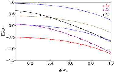
Figure 2: (Color online). Energies of bound states for different coupling strength $g$. The points represent bound state energies obtained by the Brillouin-Wigner perturbation theory (BWPT) when the length of the SC is long enough. The solid lines represent results obtained via numerical diagonalization for the SC with $N=7$. The total energy $E_{\rm{in}}$ of the single-photon scattering process is in the range between two blue dashed lines. The brown dash-dotted line stands for the upper limit of $E_{2}$ for the inelastic scattering process. Here we take $\omega_{a}/\omega_{c}=1$ and $\xi/\omega_{c}=0.23$ in units of $\omega_{c}=1$.

Compared to the numerical diagonalization method, the utilization of the BWPT can save the time to identify the bound states and the internal storage in calculation under the same condition. Thus we use the BWPT to get the three lowest energy levels of the bound states, which are shown by points in Fig. 2, when the length of the SC is long enough. The convergence of our results is examined in Appendix A.2. As shown in Fig. 2, we find that the ground state energies with $g$ obtained from numerical diagonalization of the Hamiltonian (2a) for the SC with $N=7$ agree well with those corresponding points. The energy of $|\psi_{2}\rangle$ is in close agreement with that obtained via the BWPT below its upper limit for the inelastic scattering process. In our numerical calculations, the excitation $\hat{N}_{\rm{ext}}$ is cut off at a given number $N_{\rm{ext}}=7$, which is found to be sufficient to guarantee the convergence of numerical results. We also find that all three bound states have certain parity and obey $\hat{P}|\psi_{0}\rangle=|\psi_{0}\rangle,\hat{P}|\psi_{1}\rangle=-|\psi_{1}\rangle,\hat{P}|\psi_{2}\rangle=|\psi_{2}\rangle$. In other words, $|\psi_{0}\rangle$ and $|\psi_{2}\rangle$ are the states with even parity and $|\psi_{1}\rangle$ is that with odd parity.

With the extended and bound states of the SC system, we can furthermore study the single-photon scattering in the full system. The single-photon scattering process in our model can be formulated as follows. Initially, we inject a photon with momentum $k_{0}$ and prepare the SC system at its ground state $|\psi_{0}\rangle$ (the lowest bound state). Absorbing the input photon with frequency $\omega_{\rm{in}}=\omega_{c}-2\xi\cos k_{0}$, the scatterer (the SC system) will jump to the extended eigenstates, which are not stable due to its coupling with the left and right channels. Then, a photon will be emitted with the carrying frequency $\omega_{\rm{out}}$, and the scatterer will pass to some bound state $|\psi_{m}\rangle$.

According to the energy conservation in the scattering process, we have

$$E_{\rm{in}}=E_{0}+\omega_{\rm{in}}=E_{m}+\omega_{\rm{out}}.$$ (7)

It implies that $\omega_{\rm{out}}=\omega_{\rm{in}}$ for the elastic scattering process ($E_{m}=E_{0}$) while $\omega_{\rm{out}}\neq\omega_{\rm{in}}$ for the inelastic scattering process ($E_{m}\neq E_{0}$). Under appropriate parameter conditions (as shown below), the two scattering processes will occur simultaneously. Furthermore, according to the conservation of the parity and the energy, the single-photon inelastic scattering for $m=2$ occurs. Therefore we get $\omega_{\rm{in}}=E_{2}-E_{0}+\omega_{\rm{out}}$ and the condition for the single-photon inelastic scattering is

$$\omega_{\rm{in}}\geq E_{2}-E_{0}+\omega_{c}-2\xi.$$ (8)

With Eq. (8), we get the upper limit of $E_{2}$ for the inelastic scattering process as $E_{0}+4\xi$, which is shown by a brown dash-dotted line in Fig. 2. This implies that the length $N=7$ of the SC is enough for our investigation of single-photon inelastic scattering.

III Numerical Results And Analysis

Now let us study the single-photon scattering process based on our model in the regimes of $\eta/\xi\in[0,1]$, in particular the two cases $\eta/\xi\ll 1$ and $\eta/\xi\approx 1$. In the single-photon scattering process, we consider only the photon states in the left channel and the right channel up to one photon, which is a good approximation when the length of the SC is sufficient long such that the multi-photon process occur only in the cavities near the atom Wang et al. (2012). In this approximation, the time-independent scattering state can be written as

$$|\Psi_{s}\rangle =|\Phi_{\rm{k_{0}}}\rangle+r_{\text{e}}|\Phi^{*}_{\rm{k_{0}}}\rangle+t_{\text{e}}|\Theta_{\rm{k_{0}}}\rangle+\sum_{m}d_{m}|\text{vac};\varphi_{m};\text{vac}\rangle$$

$$\quad{}+r_{\text{in}}|\Phi^{*}_{\rm{k_{2}}}\rangle+t_{\text{in}}|\Theta_{\rm{k_{2}}}\rangle$$ (9)

with

$$|\Phi_{\rm{k_{i}}}\rangle =\sum^{0}_{j=-\infty}e^{ijk_{i}}|j;\psi_{i};\text{vac}\rangle,$$ (10)

$$|\Theta_{\rm{k_{i}}}\rangle =\sum^{\infty}_{j=N+1}e^{ijk_{i}}|\text{vac};\psi_{i};j\rangle,~{}$$ (11)

which satisfies the Schr$\ddot{o}$dinger equation

$$\hat{H}|\Psi_{s}\rangle=E_{\rm{in}}|\Psi_{s}\rangle,$$ (12)

where the coefficients $r_{\text{e}}$ ($r_{\text{in}}$) and $t_{\text{e}}$ ($t_{\text{in}}$) in Eq. (9) represent respectively the reflection and transmission amplitudes in the elastic (inelastic) scattering channel, $d_{m}$ is the probability amplitude for the system in the state $|\text{vac};\varphi_{m};\text{vac}\rangle$, and the eigenenergy $E_{\rm{in}}=E_{0}+\omega_{c}-2\xi\cos k_{0}$. Substituting Eq. (9) into Eq. (12), we get a set of equations

$$\xi r_{\text{e}}e^{-ik_{0}}-\eta\sum_{i=0}d_{i}\langle\psi_{0}|\hat{a}_{1}|\varphi_{i}\rangle = -\xi e^{ik_{0}},$$ (13a)

$$\xi t_{\text{e}}e^{iNk_{0}}-\eta\sum_{i=0}d_{i}\langle\psi_{0}|\hat{a}_{N}|\varphi_{i}\rangle = 0,$$ (13b)

$$\xi e^{-ik_{2}}r_{\text{in}}-\eta\sum_{i=0}d_{i}\langle\psi_{2}|\hat{a}_{1}|\varphi_{i}\rangle = 0,$$ (13c)

$$\xi e^{iNk_{2}}t_{\text{in}}-\eta\sum_{i=0}d_{i}\langle\psi_{2}|\hat{a}_{N}|\varphi_{i}\rangle = 0,$$ (13d)

and

$$\begin{split}&(E_{in}-\epsilon_{j})d_{j}+\eta r_{\text{e}}\langle\varphi_{j}|\hat{a}^{\dagger}_{1}|\psi_{0}\rangle+\eta r_{\text{in}}\langle\varphi_{j}|\hat{a}^{\dagger}_{1}|\psi_{2}\rangle\\ +&\eta t_{\text{e}}e^{i(N+1)k_{0}}\langle\varphi_{j}|\hat{a}^{\dagger}_{N}|\psi_{0}\rangle+\eta t_{\text{in}}e^{i(N+1)k_{2}}\langle\varphi_{j}|\hat{a}^{\dagger}_{N}|\psi_{2}\rangle\\ =&-\eta\langle\varphi_{j}|\hat{a}^{\dagger}_{1}|\psi_{0}\rangle.\\ \end{split}$$ (14)

By numerically solving Eqs. (13) and (14), we will obtain the reflection and transmission flow in the elastic scattering channel as $J_{\rm{R,e}}=|r_{\text{e}}|^{2}$ and $J_{\rm{T,e}}=|t_{\text{e}}|^{2}$, respectively. Due to the different photon momentum in elastic and inelastic channels, the reflection and transmission flow in the inelastic scattering channel should be written as $J_{\rm{R,in}}=\left|r_{\text{in}}\right|^{2}\sin k_{2}/\sin k_{0}$ and $J_{\rm{T,in}}=\big{|}t_{\text{in}}\big{|}^{2}\sin k_{2}/\sin k_{0}$ Wang et al. (2014). Then the flow conservation relation is expressed as $J_{\rm{R,e}}+J_{\rm{T,e}}+J_{\rm{R,in}}+J_{\rm{T,in}}=1$.

III.1 Numerical results for $\eta\ll\xi$

In the regime of $\eta\ll\xi$, the SC system described by the Hamiltonian $H_{S}$ couples to the left and right channels weakly. Therefore, our whole system can be regarded as a microscopic one-dimensional Cavity-QED model without the RWA, whose transmission peaks of single-photon scattering correspond to the eigenstates $\{|\varphi_{m}\rangle\}$ that satisfy $\langle\varphi_{m}|\hat{a}^{\dagger}_{1}|\psi_{0}\rangle\neq 0$.

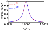
(a) $g/\omega_{c}=0.001$.

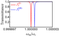
(b) Zoom in of LABEL:sub@fig:Cg001.

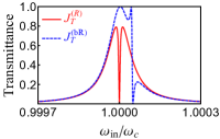
(c) $g/\omega_{c}=0.01$.

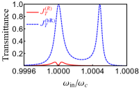
(d) $g/\omega_{c}=0.05$.

Figure 3: (Color online). The transmittance as a function of $\omega_{\rm{in}}$ at $\omega_{\rm{in}}=\omega_{c}$. The red solid line represents the transmittance $J^{\rm{(R)}}_{\rm{T}}$ in the RWA while the blue dashed line stands for $J^{\rm{(bR)}}_{\rm{T}}$ beyond the RWA. Here we take the length of the scatterer $N=7$ and $\eta/\omega_{c}=0.002$, $\xi/\omega_{c}=0.04$.

When $\xi\ll\omega_{c}$, we have $E_{0}+\omega_{\rm{in}}-E_{2}<\omega_{c}-2\xi$, which implies that only the elastic scattering process occurs due to the energy conservation. In this regime, a transmission valley induced by destructive interference between two transmission channels in the RWA was found in Ref. Zhu et al. (2014). A natural problem is to investigate whether and how the CRW term affects the transmission valley.

To this end, we compare the transmission rates in the cases with and without the CRW term $\hat{H}_{\text{int}}^{\text{CRW}}$ when the incident photon frequency $\omega_{\text{in}}$ is near $\omega_{c}$, where the atom is located in the node of the resonant mode of the SC. In Fig. 3, we plot the elastic transmission flow $J_{\rm{T,e}}$ as a function of the frequency of incident photon for $g/\omega_{c}=0.001,0.01,0.05$ in 3a, 3c, 3d respectively. In the RWA, the transmission valley becomes lower and lower as $g$ increases, and the position of the valley is invariant with $g$. The phenomena in the RWA can be understood as follows. In the RWA, the eigenenergy of the eigenstate formed by the atom coupling with the non-resonant modes of the SC is invariant, which directly leads to the invariant position of the transmission valley. As $g$ increases, this eigenstate has larger decay into the outside channels, together with the destructive interference mechanism, which explain why the transmission valley becomes lower and lower.

When consider the CRW term, we find that when $g/\omega_{c}=0.001$, there is a negligible effect of the CRW term in the transmission valley. In fact, it has a small displace of the valley position as shown in Fig. 3b. When $g/\omega_{c}=0.01$, the transmission becomes asymmetric obviously. When $g/\omega_{c}=0.05$, there appear two strong transmission peaks. The above phenomena originate from the CRW term induced eigenenergy displacement of the eigenstate formed by the atom coupling with the non-resonant modes, which is possible to be sufficiently large with respect to the decay rate of the resonant mode of the SC.

Moreover, we have also investigated the transmission spectrum when the atom is located in the antinode of the empty SC, it exhibits the normal Rabi splitting shape as expected, the RWA and full Hamiltonian give almost the same results with the same parameters $g$ as above. It means that the CRW term does not contribute significantly to the dynamics of the system when the atom is not located in the node of the resonant mode of the SC, in contrary to the case when the atom is located in the node.

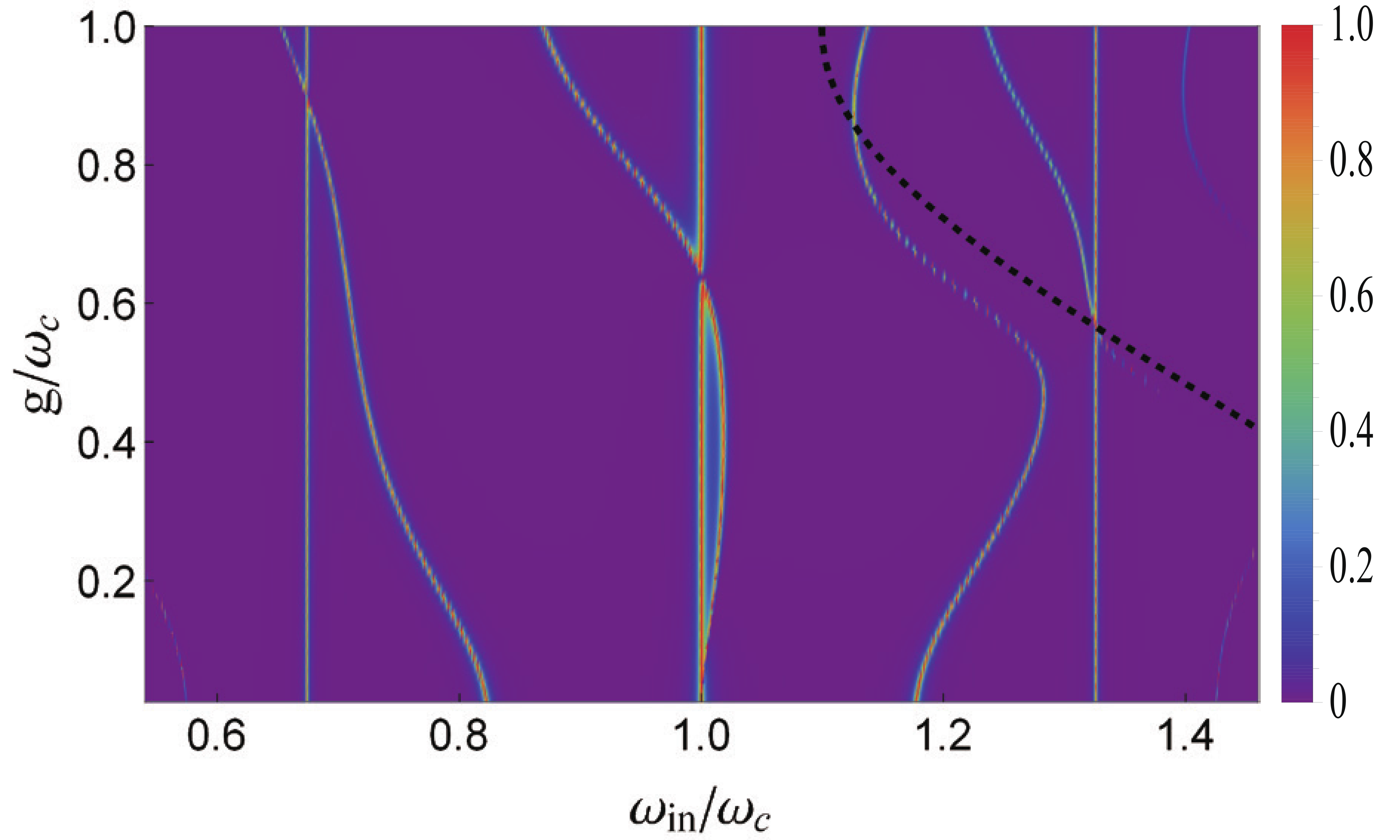
(a) The total transmittance $J_{\text{T}}$.

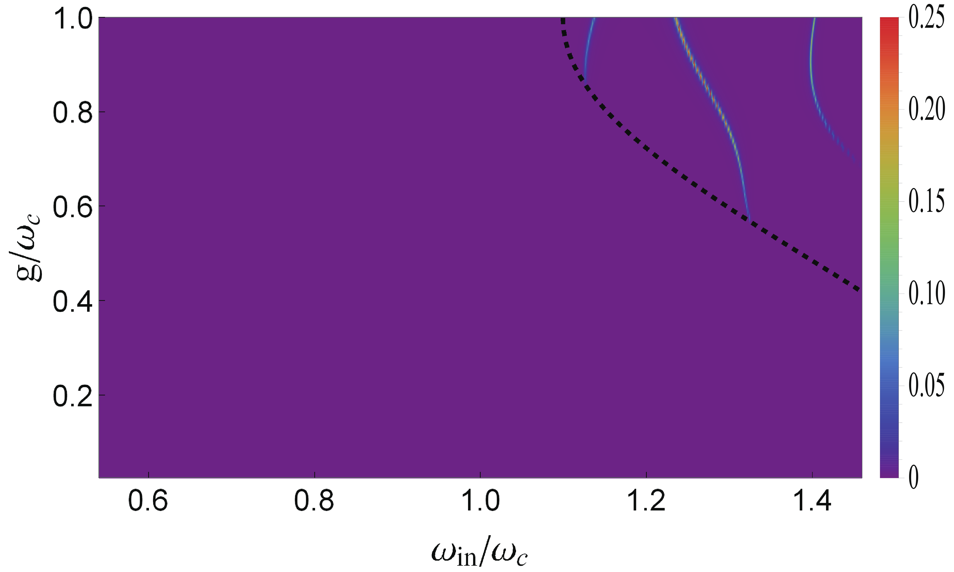
(b) The inelastic transmittance $J_{\text{T,in}}$.

Figure 4: (Color online). Transmittance as a function of incident photon frequency $\omega_{in}$ and $g$ for $\eta=0.03\omega_{c},~{}\xi=0.23\omega_{c}$. The black dashed line marks the estimated frequency given by Eq. (8).

Now, let us come to the parameter regime in which $\xi$ is in the same order of $\omega_{c}$. In Fig. 4 the total transmission spectrum $J_{\rm{T}}=J_{\rm{T,e}}+J_{\rm{T,in}}$ and the inelastic one $J_{\rm{T,in}}$ are shown for the SC-QED model. In Fig. 4b, we observe the inelastic scattering when the condition Eq. (8) is satisfied and $J_{\rm{T,in}}$ exceeds $10\%$ for larger $g/\omega_{c}$ which indicates that it can be easily observed in experiments. Furthermore, these inelastic scattering peaks must be associated with an extended state $|\varphi_{m}\rangle$ which satisfies $\langle\psi_{2}|\hat{a}_{N}|\varphi_{m}\rangle\langle\varphi_{m}|\hat{a}^{\dagger}_{1}|\psi_{0}\rangle\neq 0$.

In Fig. 4a, we find that the location of some peaks are the same which implies that the energy gaps between the associated states and the ground states are not changed for different $g$. To find the corresponding states, we rewrite the Hamiltonian (2a) into

$$\begin{split}\hat{H}_{S}=&\sum_{k}[\omega_{c}-2\xi\cos(\frac{k\pi}{N+1})]\hat{b}^{\dagger}_{k}\hat{b}_{k}+\frac{\omega_{a}}{2}\hat{\sigma}_{z}\\ &+\sum_{k}G_{k}\hat{\sigma}_{x}(\hat{b}^{\dagger}_{k}+\hat{b}_{k}),\end{split}$$ (15)

where

$$\hat{b}^{\dagger}_{k} =\sqrt{\frac{2}{N+1}}\sum^{N}_{j=1}\sin(j\frac{k\pi}{N+1})\hat{a}^{\dagger}_{j},$$ (16)

$$G_{k} =g\sqrt{\frac{2}{N+1}}\sin(\frac{k\pi}{2}).$$ (17)

For $k^{\prime}$ satisfying $G_{k^{\prime}}=0$, we have

$$\hat{H}_{S}b^{\dagger}_{k^{\prime}}|\psi_{0}\rangle=\left(E_{0}+\omega_{c}-2\xi\cos\left(\frac{k^{\prime}\pi}{N+1}\right)\right)b_{k^{\prime}}^{\dagger}|\psi_{0}\rangle.$$ (18)

In the case of $N=7$, $G_{k^{\prime}}=0$ will give $k^{\prime}=2,4,6$, and the energy gaps of the states $b^{\dagger}_{k^{\prime}}|\psi_{0}\rangle$ with respect to the ground states are $\omega_{c}-2\xi\cos\frac{k^{\prime}\pi}{8}$, independent of the coupling strength $g$, which contribute to the straight transmission lines as shown in Fig. 4a. Moreover, by comparing Fig. 4a with Fig. 4b, we find that these states make no contributions to the inelastic scattering because $\langle\psi_{2}|\hat{a}_{N}b^{\dagger}_{k^{\prime}}|\psi_{0}\rangle\approx 0$ although $\langle\psi_{0}|\hat{b}_{k^{\prime}}\hat{a}^{\dagger}_{1}|\psi_{0}\rangle\neq 0$.

Notice that in Fig. 4a, a significant transmission valley appears near every intersection of two transmission lines, which implies there are two transmission channels for the photon. The transmission valley is from the destructive interference between these two channels: one is provided by the state $b^{\dagger}_{k^{\prime}}|\psi_{0}\rangle$, while the other results from the atom coupling with the non-resonant modes of the SC. The physics is the same as that we analyzed in the case $\eta\ll\xi\ll\omega_{c}$.

III.2 Numerical results for larger $\eta/\xi$

As the parameter $\eta$ increases, the coupling between the SC system and the left and the right channels increases. In particular, when $\eta=\xi$, the border between the SC system and the outside channels disappears, and the length of the SC system is artificial. In this case, the SC system acts as the scattering region, where the multi-photon processes occur. In the outside channels, we only consider the single photon process. This approximation can be identified by numerically checking the convergence of the transmittance by choosing a longer length of the SC.

In Fig. 5, our numerical results for the total transmittance $J_{\rm{T}}$ and the inelastic transmittance $J_{\rm{T,in}}$ are plotted in 5a and 5b respectively as functions of $\eta$ and $\omega_{\text{in}}$ when $g=0.6\omega_{c}$.

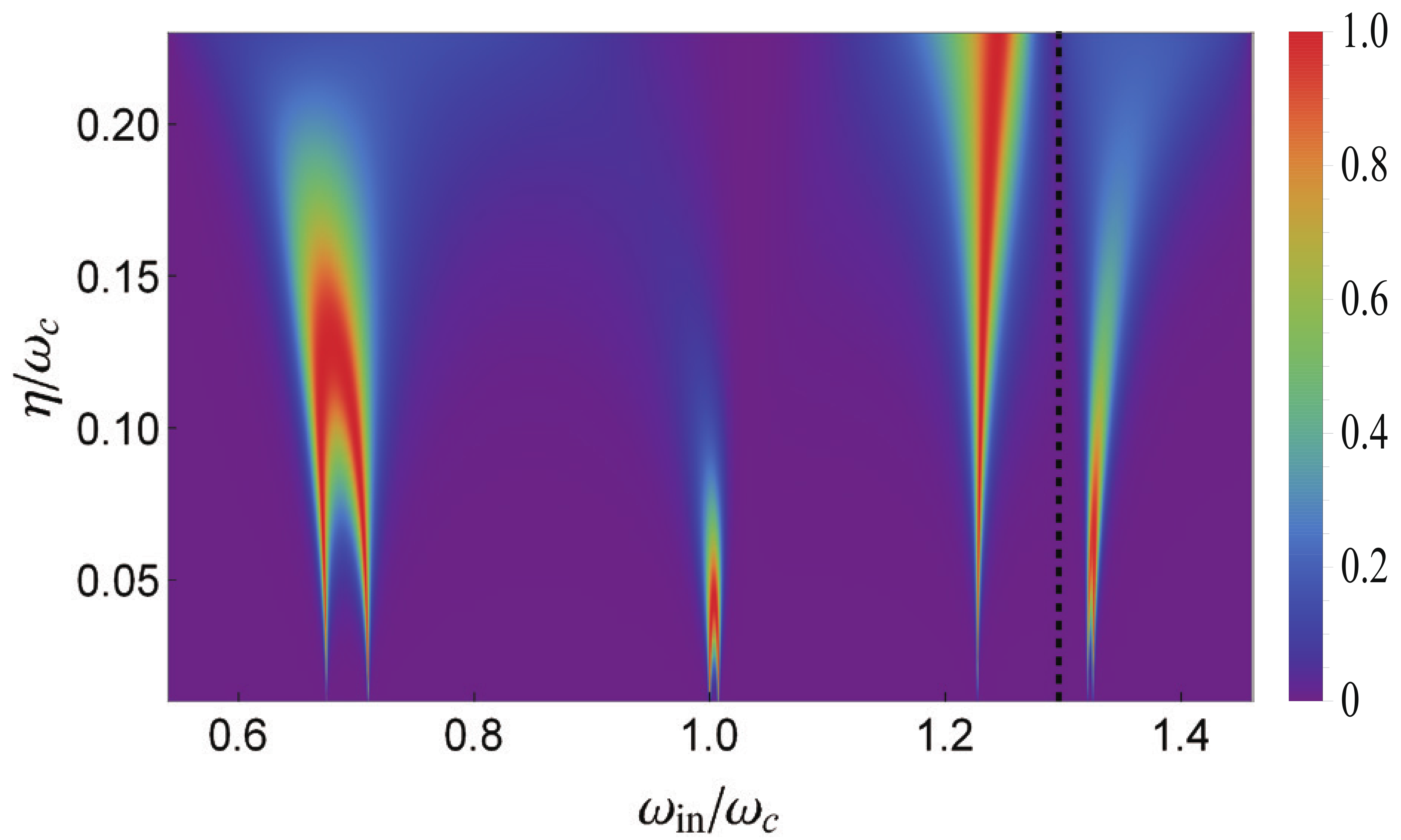
(a) The total transmittance $J_{\text{T}}$.

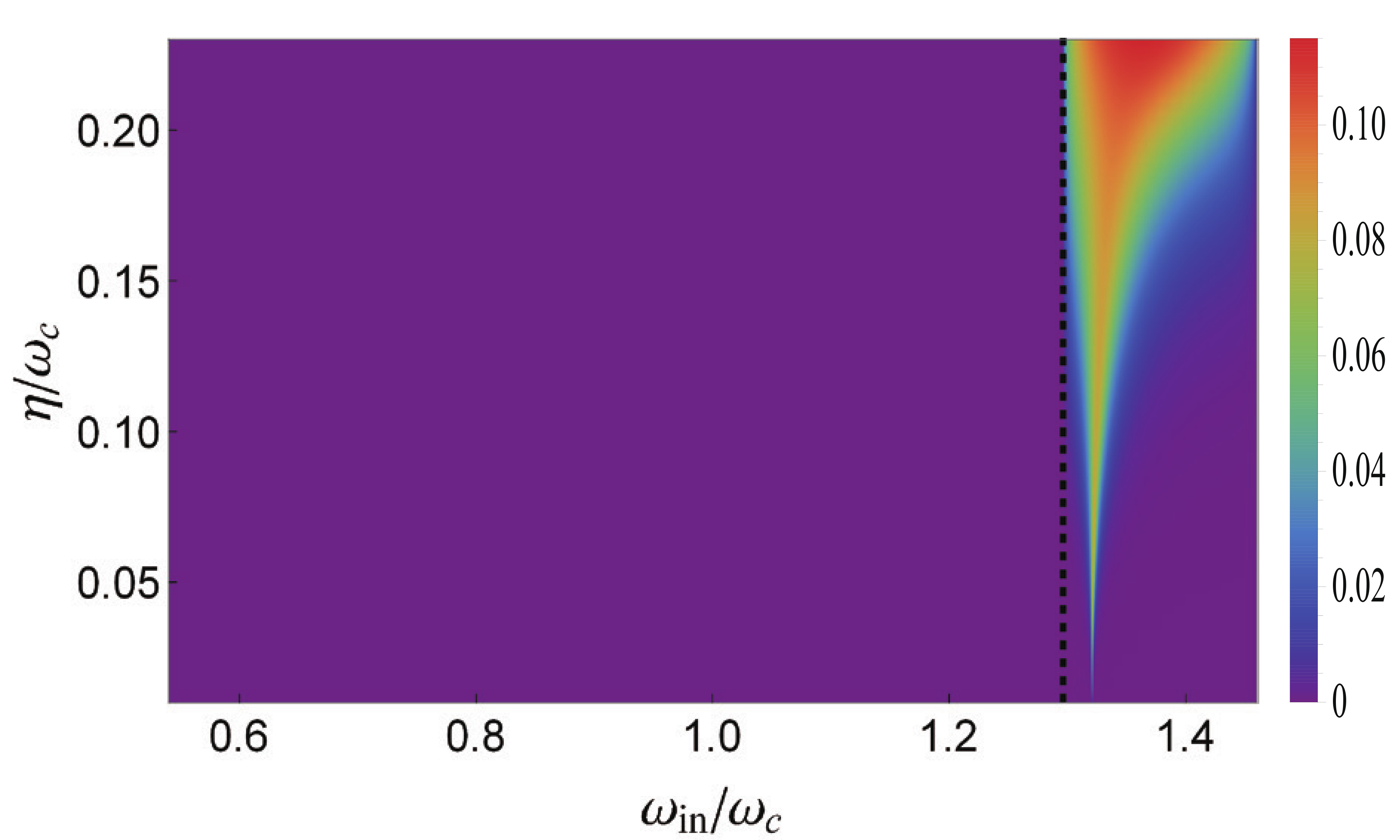
(b) The inelastic transmittance $J_{\text{T,in}}$.

Figure 5: (Color online). Transmittance as a function of incident photon frequency $\omega_{in}$ and $\eta$. The black dashed line marks the frequency given by Eq. (9). Here, we take $g/\omega_{c}=0.6$ and choose the length of the SC $N=7$.

As shown in Fig. 5a, the transmission spectrum for $\eta\ll\xi$ can be explained with the analysis in Sec. III.1. As $\eta$ gets larger, the peak of transmittance gets wider as expected. When $\eta/\xi$ becomes larger, several peaks are mixed, and the corresponding eigenstates becomes indistinguishable from the transmission spectrum. As $\eta/\xi$ becomes sufficient large, only one transmission peak remains while the other peaks dilute in the continuous spectrum. This peak implies a resonant state appearing in our system.

In Fig. 5b, the inelastic transmittance occurs when the condition in Eq. (8) is satisfied. As $\eta$ is small, there is an inelastic peak. As $\eta$ increases, the peak develops into a continuous spectrum.

In order to study the properties of transmittance for larger $\eta/\xi$, we choose $\eta=\xi$ to plot the total transmittance $J_{\rm{T}}$ and the inelastic transmittance $J_{\rm{T,in}}$ in Figs. 6a and 6b respectively.

If the RWA is introduced to the model, the minimum of the elastic transmittance is at $\omega_{min}=\omega_{c}$. However, for sufficiently large $g/\omega_{c}$, the CRW term will cause the shift of the minimum frequency which is shown by a white solid line in Fig. 6a. This phenomenon has also been observed in Ref. Sanchez-Burillo et al. (2014).

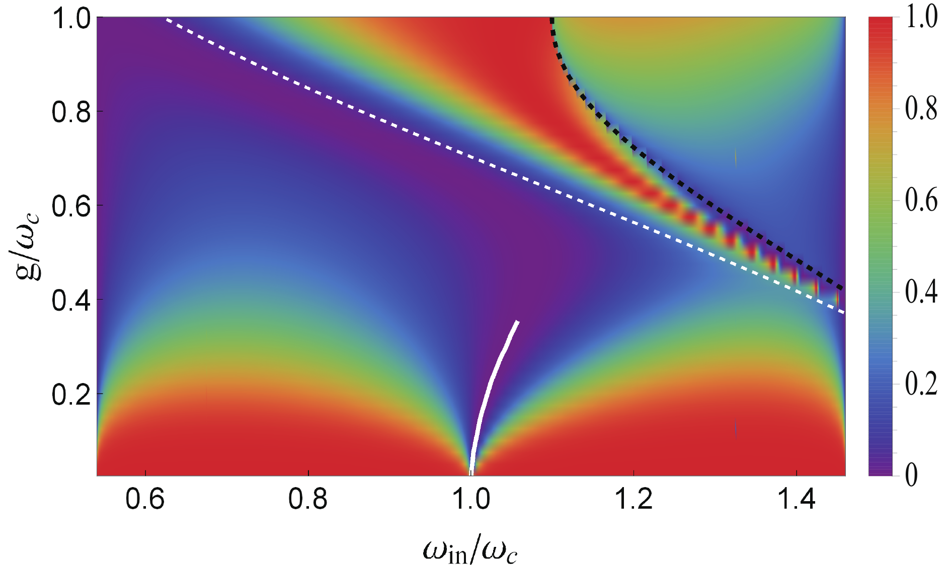
(a) The total transmittance $J_{\text{T}}$.

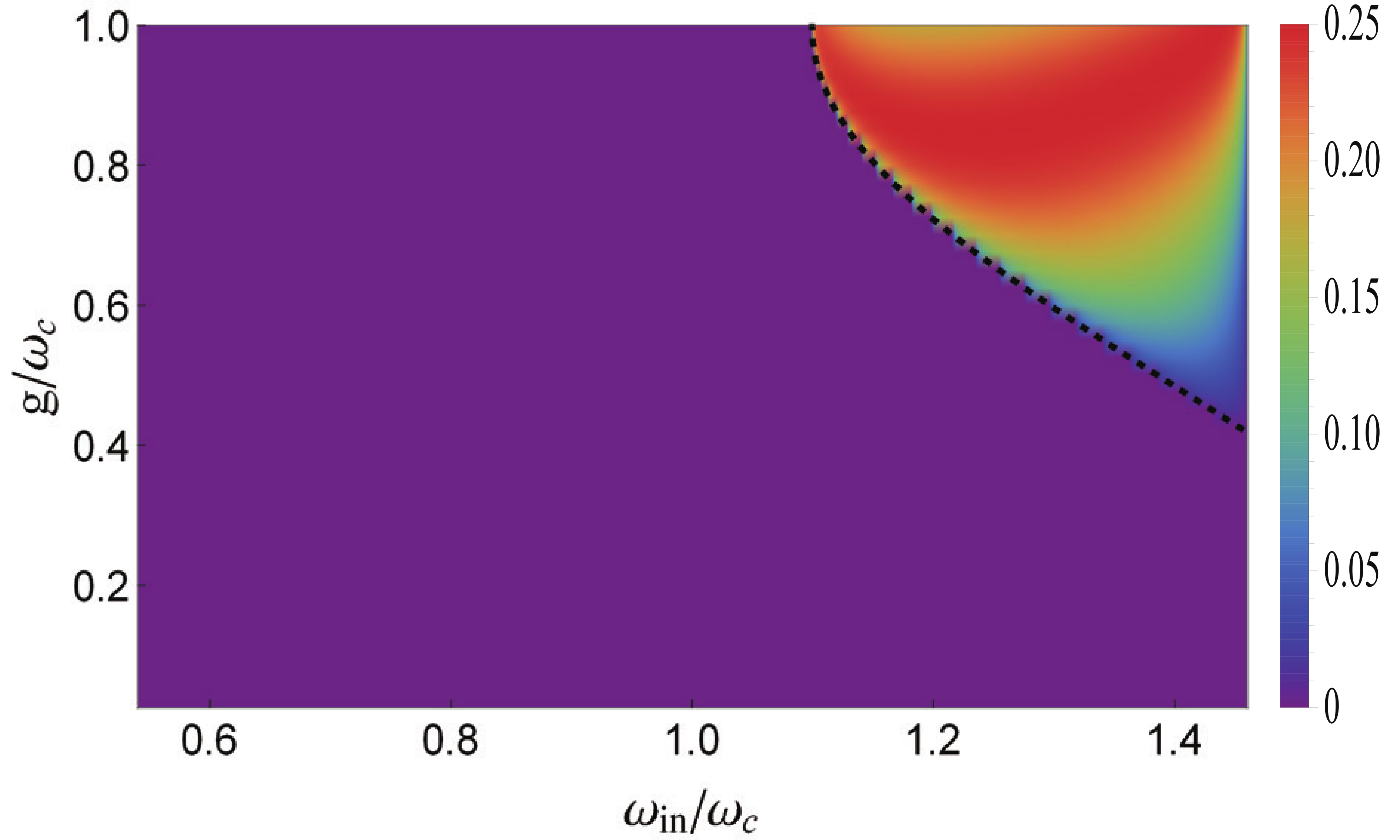
(b) The inelastic transmittance $J_{\text{T,in}}$.

Figure 6: (Color online). Transmittance as a function of incident photon frequency $\omega_{in}$ and $g$ for $\eta=\xi=0.23\omega_{c}$. The white solid line represents the minimum of the elastic transmittance. The white dashed line stands for the energy of a bound state, relative to the ground state energy $E_{0}$, obtained via the numerical diagnolization. And the black dashed line marks the estimated frequency given by Eq. (8).

Applying the exact diagonalization in the subspace with the excitation number $N_{\text{ext}}\geq 3$ of the Hamiltonian (2a), we obtain a white dashed line in Fig. 6a, which represents the energy of a state with odd parity relative to $E_{0}$. This state is a bound state of the subspace which would be proved in Appendix B. Since it enters into the single-photon scattering energy regime and couples with single excitation states, it generates a resonant state Cohen-Tannoudji et al. (1998), which would induce the Fano-type resonance Fano (1961) in Fig. 6a as mentioned above. Notice that this resonant state is not a bound state based on Appendix A, although its spatial profile of the photon excitations has localized shape.

In Fig. 5a we demonstrate how a transmission spectrum at $g/\omega_{c}=0.6$ in Fig. 4a is transformed into that in Fig. 6a. The transmission line near $\omega_{\text{in}}/\omega_{c}\simeq 1.2$ corresponds to the above resonant quasi-bound state. We find that this quasi-bound state has a significant component with three excitations, which makes it weakly coupled with the outside channels, and hence it has a long life time.

Furthermore, the black dashed line in Figs. 5b and 6b shows the lower energy limit of the incident photon to observe the inelastic scattering phenomenon. In our case, the inelastic transmittance never exceeds $25\%$, and the inelastic reflectance equals to the inelastic transmittance due to the symmetry of our model.

IV Conclusion

In this article, we have investigated the single-photon scattering process via a SC-QED system with the Hamiltonian in Eq. (1) and Eqs. (2). Since the Hamiltonian contains the CRW term in Eq. (5), it is suitable to study the physics of the ultrastrong coupling regime. In our study, the parameter $\eta$ varies in the region $0<\eta/\xi\leq 1$. When $\eta/\xi\ll 1$, it describes a SC-QED system. When $\eta=\xi$, it describes a waveguide QED system. We find that the condition for the single-photon scattering is satisfied in our model, which gives us a good opportunity to study the crossover between these two regimes. In these two regimes, we have studied how the coupling between the atom and one cavity affects the transmission. Technically, we present a time independent scattering theory to describe these single-photon scattering processes, in which the bound states in the scattering region play an important role. In the microscopic mechanism to give rise to the inelastic process or to produce the Fano-type resonance, the bound states or the quasi-bound states play an essential role.

More precisely, we have predicted the following phenomena for the transmission spectra. As shown in Fig. 3, the CRW contribution could be detected even in the weak atom-cavity coupling regime when the atom is at the node of the resonant of the empty SC system for $\eta\ll\xi\ll\omega_{c}$. Besides, the CRW induced inelastic scattering in Figs. 4b, 5b and 6b will not appear until Eq. (8) is satisfied. By tuning the ratio $\eta/\xi$, we can take Fig. 5 as an example to investigate the single-photon scattering problem in the crossover from a SC-QED ($\eta\ll\xi$) to a waveguide QED ($\eta=\xi$). For the case that $\eta=\xi$, the blueshift of the elastic transmittance minimum, which has also been observed in Ref. Sanchez-Burillo et al. (2014), can be obtained based on our proposed mechanism. Meanwhile, the Fano-type resonance Fano (1961) in Fig. 6a has been interpreted as the result of a long-lived quasi-bound state. Further more, the inelastic scattering phenomena can be obviously observed for sufficiently large $g/\omega_{c}$.

In summary, we present a unified framework to study the single photon transmission phenomena induced by the CRW term $\hat{H}^{\rm{CRW}}_{\rm{int}}$ in our model for any coupling strengths $\eta/\xi\in(0,1]$ and $g/\omega_{c}\in[0,1]$. Our results provide theoretical foundations to manipulate the CRW effects in the corresponding realistic systems. Besides, although the single-photon scattering condition is satisfied, the multi-photon processes in the scattering region play a key role in the effects from the CRW term. We hope that our work will stimulate the further studies on multi-photon scattering effects induced by the CRW interaction in many diverse systems.

Appendix A Bound states analyzed with BWPT 

A.1 The origin of bound states 

To study the bound state, we have resort to Brillouin-Wigner perturbation theory Hubač and Wilson (2010) instead of the Rayleigh-Schr$\ddot{o}$dinger perturbation theory Sakurai and Napolitano (2011) in that the former will essentially avoid the possible divergences.

First we divide the Hamiltonian (2a) into two parts, $\hat{H}_{S}=\hat{H}_{0}+\hat{V}$, where

$$\hat{H}_{0}=\omega_{c}\sum^{N}_{j=1}\hat{a}^{\dagger}_{j}\hat{a}_{j}+\frac{\omega_{a}}{2}\hat{\sigma}_{z}+g\hat{\sigma}_{x}(\hat{a}^{\dagger}_{s}+\hat{a}_{s})$$ (19)

is the free Hamiltonian, and

$$\hat{V}=-\xi\sum^{N}_{j=2}(\hat{a}^{\dagger}_{j}\hat{a}_{j-1}+\hat{a}^{\dagger}_{j-1}\hat{a}_{j})$$ (20)

is treated as a perturbation.

In the free Hamiltonian $\hat{H}_{0}$, the $s$-th cavity and the two-level atom forms the Rabi model, which has been analytically solved recently in Ref. Braak (2011). Most eigenstates of $\hat{H}_{0}$ are highly degenerate, and the non-degenerate eigenstates are given by

$$|\psi_{m,P}^{(0)}\rangle=|\phi_{m,P}\rangle\otimes_{j=1}^{s-1}|0\rangle_{j}\otimes_{j=s+1}^{N}|0\rangle_{j}$$ (21)

for $m\in\{1,2,\cdots\}$, where $|\phi_{m,P}\rangle$ is the $m$-th eigenstate in the subspace with even parity ($P=1$) or odd parity ($P=-1$) of the Rabi model, and $|0\rangle_{j}$ is the state with $0$ photon in the $j$-th cavity.

Note that the bound states here are the eigenstates of $H_{S}$ where the photon excitation is localized near the middle of the cavity array. In this sense the zero order eigenstates $\{|\psi_{m,P}^{(0)}\rangle\}$ are bound states when $\xi=0$. Since $\{|\psi_{m,P}^{0}\rangle\}$ are non-degenerate, it is reasonable for us to expect that when $\xi$ is not very large, the corresponding eigenstates $\{|\psi_{m,P}\rangle\}$ are still bound states with parity unchanged.

A.2 Examination of convergence of numerical results

As we know, when the length $N$ of the SC is long enough, the energy of a bound state in the SC system should be almost independent of $N$. Considering the constraint of computational resources, we have to find a proper $N$ to obtain the highly accurate energy of the bound state, which implies the necessity of examinating the convergence of our results. Here, we take the ratio of the photon number in the $N$-th cavity to the total photon excitation number as reference and show this ratio as a function of coupling strength $g$ for different length $N$ in Fig. 7.

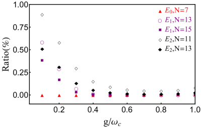
Figure 7: (Color online). The ratio of the photon number in the $N$-th cavity to the total photon excitation number of the bound states as a function of the coupling strength $g$ for different length $N$ of the SC. Here we show the results of the ground state with $N=7$ (red filled triangles), the first excited bound state with $N=13$ (purple empty circles) and $N=15$ (purple filled squares), the second excited bound state with $N=9$ (black empty diamonds) and $N=11$ (black filled diamonds).

As shown in Fig. 7, the ratio equals to zero for the ground state, which indicates that $N=7$ is enough to obtain $E_{0}$. We also find that for higher energy levels, the ratio decreases with the increase of $g$ and $N$. In order to guarantee the convergence, we use the BWPT to get $E_{1}$ with $N=15$ and $E_{2}$ with $N=13$ in the main text Fig. 2 to ensure the ratio less than $1\%$.

Appendix B The bound state of the subspace

In the subspace with the excitation number $N_{\text{ext}}\geq 3$ of the Hamiltonian (2a), we can obtain a state with the lowest energy via numerical diagonalization. The energy of this state as a function of coupling strength $g$ for different length of the SC are shown in Fig. 8.

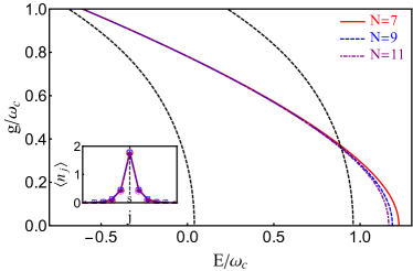
Figure 8: (Color online). The lowest eigenenergy of the subspace with the excitation number $N_{\text{ext}}\geq 3$. Dependence with coupling strength $g$ and the length $N$ of the SC. The red solid line, the blue dashed line and the purple dash-dotted line represent respectively results for $N=7$, $N=9$ and $N=11$. The single-photon scattering energy regime is the range between two black dashed lines. The inset shows the spacial profile of the photon excitations in the state, for $g=0.6\omega_{c}$.

As shown in Fig. 8, when the coupling strength $g$ is large enough, the variation of energies with $g$ becomes independent of the length $N$ of the SC, and its spatial profile of the photon excitations has localized shape, which implies that it’s a bound state in this regime.

References

- Niemczyk et al. (2010) T. Niemczyk, F. Deppe, H. Huebl, E. P. Menzel, F. Hocke, M. J. Schwarz, J. J. Garcia-Ripoll, D. Zueco, T. Hummer, E. Solano, A. Marx, and R. Gross, Nat Phys 6, 772 (2010).
- Forn-Díaz et al. (2010) P. Forn-Díaz, J. Lisenfeld, D. Marcos, J. J. García-Ripoll, E. Solano, C. J. P. M. Harmans, and J. E. Mooij, Phys. Rev. Lett. 105, 237001 (2010).
- Baust et al. (2016) A. Baust, E. Hoffmann, M. Haeberlein, M. J. Schwarz, P. Eder, J. Goetz, F. Wulschner, E. Xie, L. Zhong, F. Quijandría, D. Zueco, J.-J. G. Ripoll, L. García-Álvarez, G. Romero, E. Solano, K. G. Fedorov, E. P. Menzel, F. Deppe, A. Marx, and R. Gross, Phys. Rev. B 93, 214501 (2016).
- Scalari et al. (2012) G. Scalari, C. Maissen, D. Turčinková, D. Hagenmüller, S. De Liberato, C. Ciuti, C. Reichl, D. Schuh, W. Wegscheider, M. Beck, and J. Faist, Science 335, 1323 (2012).
- Schwartz et al. (2011) T. Schwartz, J. A. Hutchison, C. Genet, and T. W. Ebbesen, Phys. Rev. Lett. 106, 196405 (2011).
- Geiser et al. (2012) M. Geiser, F. Castellano, G. Scalari, M. Beck, L. Nevou, and J. Faist, Phys. Rev. Lett. 108, 106402 (2012).
- Jaynes and Cummings (1963) E. T. Jaynes and F. W. Cummings, Proc. IEEE 51, 89 (1963).
- Irish (2007) E. K. Irish, Phys. Rev. Lett. 99, 173601 (2007).
- Braak (2011) D. Braak, Phys. Rev. Lett. 107, 100401 (2011).
- Verstraete et al. (2008) F. Verstraete, V. Murg, and J. Cirac, Adv. Phys. 57, 143 (2008).
- García-Ripoll (2006) J. J. García-Ripoll, New J. Phys. 8, 305 (2006).
- Shen and Fan (2005) J.-T. Shen and S. Fan, Phys. Rev. Lett. 95, 213001 (2005).
- Zhou et al. (2008) L. Zhou, Z. R. Gong, Y.-x. Liu, C. P. Sun, and F. Nori, Phys. Rev. Lett. 101, 100501 (2008).
- Zhu et al. (2014) W. Zhu, Z. H. Wang, and D. L. Zhou, Phys. Rev. A 90, 043828 (2014).
- Gong et al. (2008) Z. R. Gong, H. Ian, L. Zhou, and C. P. Sun, Phys. Rev. A 78, 053806 (2008).
- Wang et al. (2012) Z. H. Wang, Y. Li, D. L. Zhou, C. P. Sun, and P. Zhang, Phys. Rev. A 86, 023824 (2012).
- Sanchez-Burillo et al. (2014) E. Sanchez-Burillo, D. Zueco, J. J. Garcia-Ripoll, and L. Martin-Moreno, Phys. Rev. Lett. 113, 263604 (2014).
- Hubač and Wilson (2010) I. Hubač and S. Wilson, “Brillouin-wigner methods for many-body systems,” (Springer Netherlands, Dordrecht, 2010) Chap. Brillouin-Wigner Perturbation Theory, pp. 37–68.
- Zhang and Dong (2010) J. M. Zhang and R. X. Dong, Eur. J. Phys. 31, 591 (2010).
- Wang et al. (2014) Z. H. Wang, L. Zhou, Y. Li, and C. P. Sun, Phys. Rev. A 89, 053813 (2014).
- Cohen-Tannoudji et al. (1998) C. Cohen-Tannoudji, J. Dupont-Roc, and G. Grynberg, Atom-Photon Interactions: Basic Processes and Applications (John Wiley & Sons, 1998) pp. 49–66.
- Fano (1961) U. Fano, Phys. Rev. 124, 1866 (1961).
- Sakurai and Napolitano (2011) J. J. Sakurai and J. J. Napolitano, Modern Quantum Mechanics, 2nd Edition (Addison-Wesley & Pearson, 2011) pp. 303–321.