Unconditional Stability for Multistep ImEx Schemes: Theory

Abstract

This paper presents a new class of high order linear ImEx multistep schemes with large regions of unconditional stability. Unconditional stability is a desirable property of a time stepping scheme, as it allows the choice of time step solely based on accuracy considerations. Of particular interest are problems for which both the implicit and explicit parts of the ImEx splitting are stiff. Such splittings can arise, for example, in variable-coefficient problems, or the incompressible Navier-Stokes equations. To characterize the new ImEx schemes, an unconditional stability region is introduced, which plays a role analogous to that of the stability region in conventional multistep methods. Moreover, computable quantities (such as a numerical range) are provided that guarantee an unconditionally stable scheme for a proposed implicit-explicit matrix splitting. The new approach is illustrated with several examples. Coefficients of the new schemes up to fifth order are provided.

Keywords: Linear Multistep ImEx, Unconditional stability, ImEx Stability, High order time stepping.

AMS Subject Classifications: 65L04, 65L06, 65L07, 65M12.

1 Introduction

When a stiff differential equation is solved via an explicit time stepping scheme, stability requires time steps that are much smaller than imposed by accuracy. Implicit schemes can overcome this limitation. Unfortunately, for many practical problems, a fully implicit treatment may be structurally difficult or computationally costly. Implicit-Explicit (ImEx) methods are based on splitting the problem into two parts, one to be treated implicitly, and the other explicitly. In many problems, the stiff modes can be conveniently treated implicitly, while the explicitly treated modes are non-stiff. Moreover, for many ImEx schemes a time step restriction is incurred from the explicit part, which is generally acceptable if it is non-stiff.

The study presented here is motivated by a different situation, namely the case where an ImEx splitting is conducted for which both parts are stiff (see §1.2 for examples in which this structure arises naturally). In that case, a time step restriction based on the explicit part is not acceptable. We therefore aim for more, namely that the ImEx time stepping scheme, for the particular splitting, be unconditionally stable, i.e., arbitrarily large time steps can be chosen without losing stability.

At first glance it may sound impossible to achieve unconditional stability if some parts of the problem are treated explicitly. The reason why it is possible is that the ImEx scheme is applied to problems and splitting choices that possess specific properties, so that the implicit part can stabilize any growing modes produced by the explicit part. This concept goes further than one may think: a properly chosen ImEx scheme can stabilize a large explicit part via a smaller implicit part (see §5.1).

While the task outlined above is of interest for any time stepping scheme, this paper focuses on ImEx linear multistep methods (LMMs) [8, 15, 50]. These achieve a high order of accuracy by using information from previous time steps. Thus, in each time step, they need a single evaluation of the explicit part, and a single solve with the implicit part (chapter II.3, pg. 171 [29]). Because high order multistep methods tend to possess less favorable stability properties than Runge-Kutta methods, the task of achieving unconditional stability is of particular importance.

1.1 Outline of the problem and contributions of this paper

The problem of interest is a linear system of ordinary differential equations

$$\mbox{\boldmath$u$}_{t}=\mbox{\boldmath$L$}\mbox{\boldmath$u$}+\mbox{\boldmath$f$}(t)\quad\text{with}\quad\mbox{\boldmath$u$}(0)=\mbox{\boldmath$u$}_{0}\;,$$ (1.1)

where $\mbox{\boldmath$u$}(t),\mbox{\boldmath$u$}_{0},\mbox{\boldmath$f$}(t)\in\mathbb{R}^{N}$ and $\mbox{\boldmath$L$}\in\mathbb{R}^{N\times N}$ is a matrix. We assume that $L$ is stable, i.e., the homogeneous equation $\mbox{\boldmath$u$}_{t}=\mbox{\boldmath$L$}\mbox{\boldmath$u$}$ has solutions that remain bounded for all time (stability is independent of the forcing $f$). The term $L$$u$ in problem (1.1) is now split into an implicit part ($A$$u$) and an explicit part ($B$$u$), transforming (1.1) into

$$\mbox{\boldmath$u$}_{t}=\mbox{\boldmath$A$}\mbox{\boldmath$u$}+\mbox{\boldmath$B$}\mbox{\boldmath$u$}+\mbox{\boldmath$f$}(t)\;,$$ (1.2)

where $\mbox{\boldmath$B$}\mbox{\boldmath$u$}=\mbox{\boldmath$L$}\mbox{\boldmath$u$}-\mbox{\boldmath$A$}\mbox{\boldmath$u$}$.

Of course, the choice of splitting $\mbox{\boldmath$L$}=\mbox{\boldmath$A$}+\mbox{\boldmath$B$}$ is not unique. One approach is to choose $A$ as the stiff terms in $L$ (i.e., the terms that would give rise to unnecessarily small time step restrictions if treated explicitly) and $B$ as the non-stiff terms in $L$. In such a case, one can guarantee stability for an ImEx LMM [20] by requiring a time step restriction roughly dictated by an explicit treatment of $B$. However, as outlined above, here we are concerned with the situation where such a splitting strategy is not feasible/practical. Hence, we seek for ImEx time stepping schemes that are unconditionally stable when applied to (1.2), where $B$ can involve stiff terms.

Whether a time stepping scheme (of whatever kind) for (1.1) or (1.2) is stable, depends on both the scheme and the problem’s right-hand side $L$. A classical approach (for non-ImEx schemes) in stability analysis (chapter 7, [39]) is to separate stability into a property of the scheme and another property of the problem’s right-hand side, as follows. For a linear scheme, the region of absolute stability $S\subset\mathbb{C}$ is the set of all $z=k\lambda$, where $k$ is the time step, for which the numerical solution remains bounded when applied to the test equation $u_{t}=\lambda u$. Similarly, one can define a region of unconditional stability $S_{\text{u}}=\{z\in\mathbb{C}\,:\,\mu z\in S\,\;\forall\mu\geq 0\}$ as the largest cone contained within $S$. If the eigenvalues of $L$ lie in $S_{\text{u}}$, then the scheme is unconditionally stable. This concept decouples the scheme stability analysis from the detailed properties of $L$, relying on its spectrum $\sigma(\mbox{\boldmath$L$})$ only. Moreover, it allows one to make stability statements about whole classes of problems. For instance, if $S_{\text{u}}$ is the cone $|\theta-\pi|<\alpha$, where $0<\alpha<\pi/2$ and $\theta$ is the polar angle (i.e., the scheme is $A(\alpha)$ stable), then the scheme is unconditionally stable for all problems where $L$ is negative definite. Conversely, we know that the same scheme is not unconditionally stable if $L$ is skew-symmetric.

In this paper, an analogous concept is developed for the ImEx framework. This extension is not straightforward, because one now has two right-hand side operators $A$ and $B$ that, in general, do not commute and thus do not share a set of common eigenvectors (see §1.3 for references to the commutative case).

While the fundamental idea of stability criteria for ImEx schemes has been presented before (see §1.3), here we present sufficient criteria for unconditional stability that are less restrictive than prior work. The stability set $\mathcal{D}$ that we introduce depends only on the coefficients of the ImEx schemes, and not the matrices $A$ and $B$ in the splitting (1.2). Moreover, we devise new high order ImEx schemes with very large stability regions that can stabilize splittings of the form (1.2) which are unstable with current schemes (see §5).

1.2 Motivating applications

While the ideas developed here apply to an abstract ODE system (1.2), particular interest lies in systems that arise from a method of lines (chapter 9.2, [39]) discretization (e.g., via finite differences, finite elements, or spectral) of linear PDE problems. Two important applications are (let $\nabla_{h}$ denote the spatial discretization of $\nabla$ in an appropriate basis with smallest length scale $h$):

1. Variable coefficient diffusion with

   $$\mbox{\boldmath$L$}\mbox{\boldmath$u$}=\nabla_{h}\cdot\big{(}d(x)\;\nabla_{h}u\big{)}\;\quad\mbox{where}\;\;d(x)>0\;.$$

   Here $L$ can be split into a constant coefficient diffusion $A$ and a variable coefficient diffusion $B$. Then, fast solvers [24, 47] can treat $A$ efficiently. However, $B$ remains stiff, because it scales the same as $A$ (i.e., like $1/h^{2}$). See §5.2 for more details.

2. Non-local operators, such as the Stokes operator in the linearized Navier-Stokes equations, whose discretization either yields a dense matrix or requires the addition of extra variables through the introduction of Lagrange multipliers,

   $$\mbox{\boldmath$L$}\mbox{\boldmath$u$}=\nu\nabla_{h}^{2}u-\nabla_{h}p\quad\text{and constraint}\quad\nabla_{h}\cdot u=0\;.$$

   A splitting where $\nu\nabla_{h}^{2}u$ is implicit can create a stiff explicit $\nabla_{h}p$, [33, 40, 45].

The theory in this paper does not directly apply to cases where $\mbox{\boldmath$L$}(\mbox{\boldmath$u$},t)$ is nonlinear or time-dependent, as arising for instance with discretizations of the Cahn-Hilliard equation [11]. However, the ideas presented below for linear splitting may nevertheless be useful in stabilizing more general splittings as well.

1.3 Existing results and the new contributions in context

The simplest ImEx scheme that can achieve unconditional stability is a first order in time combination of forward and backward Euler steps. The application to (1.2) yields

$$\frac{1}{k}\big{(}\mbox{\boldmath$u$}_{n+1}-\mbox{\boldmath$u$}_{n}\big{)}=\mbox{\boldmath$A$}\mbox{\boldmath$u$}_{n+1}+\mbox{\boldmath$B$}\mbox{\boldmath$u$}_{n}+\mbox{\boldmath$f$}(nk)\;.$$ (1.3)

Here $k>0$ is the time step, and $\mbox{\boldmath$u$}_{n}$ is the numerical solution at time $t=nk$.

First order in time schemes that achieve unconditional stability originated with Douglas and Dupont [16]. Other first order approaches are: (i) iterative schemes for steady state elliptic problems [14]; (ii) variable coefficient diffusion with spectral methods (chapter 9, [23]); (iii) non-linear convex–concave splittings for the Cahn-Hilliard equation [19]; (iv) non-local explicit terms [7]; (v) Hele-Shaw flows [21]; (vi) phase-field models [10, 18, 44, 46]; (vii) viscosity-pressure splittings in incompressible Navier-Stokes [33, 40].

A disadvantage of first order approaches is that, in addition to the low order, large error constants have been reported for stable splitting choices in dissipative equations [13], as well as dispersive equations [12].

Better accuracy requires higher order ImEx time stepping methods. Two of the most commonly used approaches, which can be applied to (1.2), are:

• CN-AB: Implicit Crank-Nicolson for $A$$u$, and explicit Adams-Bashforth extrapolation for $B$$u$.

• SBDF (Semi-implicit Backward Differentiation Formula): Implicit BDF for $A$$u$, and explicit Adams-Bashforth extrapolation for $B$$u$.

For second order schemes, unconditional stability, or at least the absence of a stiff time step restriction, have been reported in practice for the semi-implicit treatment of the incompressible Navier-Stokes equations [35, 36] and the Cahn-Hilliard equation [9]. Rigorous proofs that guarantee unconditional stability for second order ImEx schemes such as SBDF or CN-AB have been given for convex–concave splittings of gradient flow systems [22, 25, 52], a coupled Stokes-Darcy system [38] and a system with an explicit treatment of non-local terms [49]. See also [18, 51] for an interpretation of some convex–concave splittings as fully implicit schemes with a rescaled time step.

Higher order semi-implicit schemes that guarantee unconditional stability are not as well studied as their first and second order counterparts. Some third order schemes for the Navier-Stokes equations have been found that do not require a diffusion-restricted time step [35, 41]. General sufficient conditions on $A$ and $B$ guaranteeing unconditional stability for any order of SBDF have been outlined in [5] and related works [3, 4]. Specifically [3, 4, 5] assume that $A$ is negative definite and also allow for $B$ to be nonlinear. The results in [5] applied to the case where $B$ is a matrix, guarantee unconditional stability for an SBDF scheme of order $1\leq r\leq 6$, if

$$\|(-\mbox{\boldmath$A$})^{-1/2}\mbox{\boldmath$B$}(-\mbox{\boldmath$A$})^{-1/2}\|_{2}<(2^{r}-1)^{-1}.$$ (1.4)

In related work, a set of new second order ImEx coefficients was introduced in [6], allowing for a weaker upper bound in (1.4) — it can be made arbitrarily close to $1$. The unconditional stability criteria devised here are more general than previous bounds such as (1.4). Instead of prescribing norm bounds, we introduce the concept of unconditional stability diagrams for ImEx schemes. The new diagrams generalize the previous work on ImEx stability regions [20] (see also [37]) to (i) the case of unconditional stability, and (ii) the case where $A$ and $B$ do not commute. We then prescribe a set of new ImEx coefficients and show that they can achieve unconditional stability for some problems which violate (1.4) by orders of magnitude. See also chapter IV of [29] for an overview of different splitting methods for ODE integration. Other techniques for specific problems are: (i) explicit RK schemes with very large stability regions for parabolic problems [1], (ii) semi-implicit deferred correction methods [43], and (iii) semi-implicit schemes when an integration factor (matrix exponential) is easily evaluated [34, 42].

This paper is organized as follows. In §2–3 we introduce ImEx LMMs, the new criteria for unconditional stability, and the definition of the unconditional stability region. In §4 we define new ImEx coefficients, characterize their unconditional stability region, and examine their effect on the approximation error. Finally, §5 demonstrates how a small implicit term may stabilize a large explicit term. It also provides an example showing how the new coefficients may be used to stabilize splittings (1.2) that arise from a variable coefficient diffusion problem. We conclude with tables of the new ImEx coefficients in §7 so that they may be used by practitioners.

2 Mathematical foundations

The purpose of this paper is to examine ImEx LMMs (linear multistep methods) for splittings of the form (1.2), where $A$$u$ is treated implicitly, and $B$$u$ explicitly. Moreover, we are particularly interested in the case where both $A$ and $B$ are stiff, i.e., each term alone would result in severely limited time steps (due to stability) when treated explicitly. The goal is to first devise simple sufficient conditions that guarantee unconditionally stability of a time stepping scheme when applied to (1.2). We will then devise new ImEx schemes that allow one to satisfy the simple unconditional stability conditions, thereby guaranteeing an unconditionally stable scheme.

Here we restrict $A$ to be real, self-adjoint, and negative definite. Thus: $\mbox{\boldmath$A$}^{T}=\mbox{\boldmath$A$}$, and $\langle\mbox{\boldmath$x$},\mbox{\boldmath$A$}\mbox{\boldmath$x$}\rangle<0$ for all $\mbox{\boldmath$x$}\neq\mbox{\boldmath$0$}$. We use the notation

$$\langle\mbox{\boldmath$x$}\/,\,\mbox{\boldmath$y$}\rangle=\overline{\mbox{\boldmath$x$}}^{T}\mbox{\boldmath$y$}\/,\quad\mbox{and}\quad\|\mbox{\boldmath$x$}\|^{2}=\langle\mbox{\boldmath$x$}\/,\,\mbox{\boldmath$x$}\rangle\;\;\mbox{for}\;\;\mbox{\boldmath$x$}\/,\,\mbox{\boldmath$y$}\in\mathbb{C}^{N}\/.$$

Note that the restriction above, which is needed for the theoretical presentation in this paper, is not as limiting as it might seem. A self-adjoint, negative definite, matrix $A$ yields desirable properties for the efficient solution of linear systems (chapter IV, lecture 38, [48]) with coefficient matrices of the form $(\mbox{\boldmath$I$}-\gamma\mbox{\boldmath$A$})$, with $\gamma>0$. The need to solve such linear systems arises in the time stepping of LMMs, as well as for implicit Runge-Kutta schemes. Hence, even if the matrix $L$ is not symmetric (e.g.: the discretization of a dispersive wave problem), it may still be advantageous to take $A$ to be symmetric and negative definite, with $\mbox{\boldmath$B$}:=\mbox{\boldmath$L$}-\mbox{\boldmath$A$}$.

Let $\mbox{\boldmath$u$}_{n}$ be the numerical solution of (1.2) at time $t=nk$, where $k$ is the time step, and let $\mbox{\boldmath$f$}_{n}=\mbox{\boldmath$f$}(nk)$. Then a LMM with $s\geq 1\/$ steps takes the form

$$\frac{1}{k}\sum_{j=0}^{s}a_{j}\;\mbox{\boldmath$u$}_{n+j}=\sum_{j=0}^{s}\Big{(}c_{j}\;\mbox{\boldmath$A$}\mbox{\boldmath$u$}_{n+j}+b_{j}\;\mbox{\boldmath$B$}\mbox{\boldmath$u$}_{n+j}+b_{j}\mbox{\boldmath$f$}_{n+j}\Big{)}\/,$$ (2.1)

where $(a_{j}\/,\,b_{j}\/,\,c_{j})\/$, with $0\leq j\leq s\/$, are the time stepping coefficients. Here we will assume that $b_{s}=0\/$ and $a_{s},c_{s}\neq 0\/$, so that the method is implicit in $A$ and explicit in $B$ — i.e., it is an ImEx time stepping scheme. To accompany equation (2.1), one must also supply $s\/$ initial vectors $\mbox{\boldmath$u$}_{0}\/,\,\mbox{\boldmath$u$}_{1}\/,\,\ldots\,\mbox{\boldmath$u$}_{s-1}\/$.

We wish to avoid any unnecessarily small time step restriction, and therefore demand that the scheme (2.1) be unconditionally stable. That is: the solutions to (2.1), with $\mbox{\boldmath$f$}=0\/$, remain bounded for arbitrarily large time steps $k>0$. This leads to:

Definition 2.1.

(Unconditional stability) A scheme (2.1) is unconditionally stable if: when $\mbox{\boldmath$f$}=0\/$, there exists a constant $C$ such that

$$\|\mbox{\boldmath$u$}_{n}\|\leq C\,\max_{0\leq j\leq s-1}\|\mbox{\boldmath$u$}_{j}\|\/,\quad\textrm{for all}\;\;n\geq s,\;k>0\quad\textrm{and}\;\;\mbox{\boldmath$u$}_{j}\in\mathbb{R}^{N}\/,\;\;\textrm{where}\;\;0\leq j\leq s-1\/.$$

Note that $C\/$ may depend on the matrices $A$, $B$, and the coefficients $(a_{j},b_{j},c_{j})$, but is independent of the time step $k\/$, the time index $n\/$, and the initial vectors $\mbox{\boldmath$u$}_{j}$, $0\leq j\leq s-1$.

Unconditional stability is a strong requirement for ImEx LMMs, and requires the following caveat: unconditional stability is a coupled property of both the set of ImEx coefficients $(a_{j}\/,\,b_{j}\/,\,c_{j})\/$ and the matrices $(\mbox{\boldmath$A$}\/,\,\mbox{\boldmath$B$})$. Hence:

• A given set of coefficients, $(a_{j}\/,\,b_{j}\/,\,c_{j})\/$, may yield unconditional stability for some splittings $(\mbox{\boldmath$A$}\/,\,\mbox{\boldmath$B$})\/$, and not others.

• If the splitting $(\mbox{\boldmath$A$}\/,\,\mbox{\boldmath$B$})\/$ arises from the spatial discretization of a PDE, then a given set of coefficients $(a_{j}\/,\,b_{j}\/,\,c_{j})\/$ may not yield unconditional stability for all model parameters.

If the matrices $A$ and $B$ commute and are diagonalizeable, then the stability of (2.1) can be examined by using the spectra, $\sigma(\mbox{\boldmath$A$})$ and $\sigma(\mbox{\boldmath$B$})$. In this paper we do not assume that $A$ and $B$ commute. Hence we cannot rely on the existence of common eigenvectors, and must develop a different approach to study the stability of (2.1), as follows:

• We introduce an unconditional stability region/diagram $\mathcal{D}$, which is computable in terms of the scheme coefficients $(a_{j}\/,\,b_{j}\/,\,c_{j})\/$ only.

• We introduce a region in the complex plane that generalizes the notion of spectrum, and depends on the matrix splitting $(\mbox{\boldmath$A$}\/,\,\mbox{\boldmath$B$})\/$ only.

This approach gives a pathway to the design of splittings that are guaranteed to be stable for a fixed set of ImEx coefficients; or to the choosing of ImEx coefficients for which a given splitting $(\mbox{\boldmath$A$}\/,\,\mbox{\boldmath$B$})\/$ yields a stable scheme. In fact, in this paper we introduce a new class of ImEx coefficients that may be chosen to stabilize a given splitting. For these new schemes the coefficients yield diagrams that permit (arbitrarily) large regions of unconditional stability.

3 Stability for linear multistep methods

In this section we review the stability criteria for ImEx linear multistep methods (LMMs) defined by equation (2.1). Following a standard procedure (chapter III.4, [26]), one may recast the linear recursion relation (2.1) with matrix coefficients, as a single vector recursion on an $s\times N$ vector:

$$\mbox{\boldmath$V$}^{n}=\mbox{\boldmath$W$}\mbox{\boldmath$V$}^{n-1},\quad\textrm{where }\;\mbox{\boldmath$V$}^{n}:=\begin{pmatrix}\mbox{\boldmath$u$}_{n+s},\;\mbox{\boldmath$u$}_{n+s-1},\;\ldots,\;\mbox{\boldmath$u$}_{n+1}\end{pmatrix}^{T}\in\mathbb{R}^{sN}.$$ (3.1)

Here $W$ is a matrix with block structure:

$$\mbox{\boldmath$W$}=\begin{pmatrix}a_{s}-kc_{s}\mbox{\boldmath$A$}&0&0&\ldots&0\\ 0&\mbox{\boldmath$I$}&0&\ldots&0\\ 0&0&\mbox{\boldmath$I$}&\ldots&0\\ \vdots&&&\ddots&0\\ 0&0&0&\ldots&\mbox{\boldmath$I$}\end{pmatrix}^{-1}\begin{pmatrix}\mbox{\boldmath$C$}_{s-1}&\mbox{\boldmath$C$}_{s-2}&\ldots&\mbox{\boldmath$C$}_{1}&\mbox{\boldmath$C$}_{0}\\ \mbox{\boldmath$I$}&0&\ldots&0&0\\ 0&\mbox{\boldmath$I$}&\ldots&0&0\\ \vdots&&\ddots&0&0\\ 0&0&\ldots&\mbox{\boldmath$I$}&0\end{pmatrix},$$ (3.2)

where $I$ is the $N\times N$ identity matrix, and

$$\mbox{\boldmath$C$}_{j}=kc_{j}\mbox{\boldmath$A$}+kb_{j}\mbox{\boldmath$B$}-a_{j}\mbox{\boldmath$I$},\quad 0\leq j\leq s-1.$$

Recall (chapter III.4, [26], chapter V.1, [27]) that equation (3.1), and hence the scheme (2.1), is stable for a given $k$ if every semisimple eigenvalue of $W$ satisfies $|\zeta|\leq 1$, and every non-semisimple eigenvalue satisfies $|\zeta|<1$. In the case when $A$ and $B$ do not commute, the eigenvalues of $W$ depend on both: (i) the matrices $A$ and $B$, and (ii) the ImEx time stepping coefficients $(a_{j},b_{j},c_{j})$. Hence the eigenvalues of $W$ do not provide a way to characterize unconditional stability in a way analogous to that for non-ImEx schemes: Some set depending on $L$ only (e.g., its spectrum) must be included within some set that is defined by the scheme coefficients only (the unconditional stability set). In what follows we devise a strategy to get around this problem, so that conditions that guarantee unconditional stability of ImEx schemes can be formulated in a language similar to the one for non-ImEx schemes, or for ImEx schemes with commutative splits (though the set depending on $\mbox{\boldmath$L$}=\mbox{\boldmath$A$}+\mbox{\boldmath$B$}$ is no longer a spectrum).

Let $\mbox{\boldmath$V$}^{*}\neq\mbox{\boldmath$0$}$ be an eigenvector of $W$ with eigenvalue $\zeta$. Then, due to the structure of the bottom $(s-1)$ matrix blocks in $W$, $\mbox{\boldmath$V$}^{*}\in\mathbb{C}^{sN}$ has the form

$$\mbox{\boldmath$V$}^{*}=\begin{pmatrix}\zeta^{s-1}\mbox{\boldmath$v$},\;\zeta^{s-2}\mbox{\boldmath$v$},\;\ldots,\;\zeta\mbox{\boldmath$v$},\;\mbox{\boldmath$v$}\end{pmatrix}^{T},\quad\textrm{where }\mbox{\boldmath$v$}\neq\mbox{\boldmath$0$},\;\mbox{\boldmath$v$}\in\mathbb{C}^{N}.$$ (3.3)

The characteristic equation for $W$ can be rewritten in the form

$$\det(\mbox{\boldmath$W$}-\zeta\mbox{\boldmath$I$})=0\quad\Longleftrightarrow\quad\det\Big{(}\frac{1}{k}a(\zeta)\;\mbox{\boldmath$I$}-c(\zeta)\;\mbox{\boldmath$A$}-b(\zeta)\;\mbox{\boldmath$B$}\Big{)}=0.$$

where

$$a(z)=\sum_{j=0}^{s}a_{j}z^{j},\quad b(z)=\sum_{j=0}^{s-1}b_{j}z^{j},\quad c(z)=\sum_{j=0}^{s}c_{j}z^{j}$$

are polynomials determined by the time stepping coefficients $(a_{j},b_{j},c_{j})$, $0\leq j\leq s$.

Hence if $\zeta$ is an eigenvalue of $W$ (with possible algebraic multiplicity greater than one), then there always exists at least one $\mbox{\boldmath$V$}^{*}$ from (3.3) with $v$ satisfying:

$$\mbox{\boldmath$T$}(\zeta)\mbox{\boldmath$v$}=0,\quad\textrm{where }\;\mbox{\boldmath$T$}(z):=\Big{(}\frac{1}{k}a(z)\;\mbox{\boldmath$I$}-c(z)\;\mbox{\boldmath$A$}-b(z)\;\mbox{\boldmath$B$}\Big{)}.$$ (3.4)

Note that one may also arrive at equation (3.4) by substituting the normal mode ansatz $\mbox{\boldmath$u$}_{n}=\zeta^{n}\mbox{\boldmath$v$}$ into the general linear ImEx time-stepping scheme (2.1).

Clearly if $\mbox{\boldmath$T$}(z)$ is singular for $|z|<1$, then any eigenvector $\mbox{\boldmath$V$}^{*}$ of $W$ has every eigenvalue (regardless of algebraic multiplicity) $|\zeta|<1$. Conditions on $\mbox{\boldmath$T$}(z)$ for the stability of (2.1) can then be stated as follows:

Proposition 3.1.

If, for a fixed $k>0$, the matrix $\mbox{\boldmath$T$}(z)$ is non-singular for all $|z|\geq 1$, i.e., $\det\mbox{\boldmath$T$}(z)\neq 0$ for $|z|\geq 1$, then the scheme (2.1) is stable.

Remark 1.

Proposition 3.1 is not sharp as we have omitted the possibility for $\det\mbox{\boldmath$T$}(\zeta)=0$ with $|\zeta|=1$.

3.1 The stability region $\mathcal{D}$

The $N\times N$ matrix equation (3.4) still couples together both the matrices $(\mbox{\boldmath$A$}\/,\,\mbox{\boldmath$B$})$ to the scheme coefficients $(a_{j},b_{j},c_{j})$. To decouple the time stepping stability analysis (i.e., the time stepping coefficients) from the details of the ODE being solved (i.e., the matrices $A$ and $B$), we multiply (3.4) by the positive definite matrix $(-\mbox{\boldmath$A$})^{p-1}$, where $p\in\mathbb{R}$ — $p$ real is all that is needed for the analysis below to hold. In the examples in §5, we will eventually focus on $p=1\/$, as it is observed that this choice provides sufficient estimates for the test problems we consider. The stability theory obtained with other values of $p\neq 1$ may still however be of use in the numerical treatment of other PDEs, distinct from those in §5. Thus:

$$\frac{1}{k}a(\zeta)(-\mbox{\boldmath$A$})^{p-1}\mbox{\boldmath$v$}=-c(\zeta)(-\mbox{\boldmath$A$})^{p}\mbox{\boldmath$v$}+b(\zeta)(-\mbox{\boldmath$A$})^{p-1}\mbox{\boldmath$B$}\mbox{\boldmath$v$}\/.$$

Dotting through with $v$ and setting

$$y=-k\frac{\langle\mbox{\boldmath$v$},(-\mbox{\boldmath$A$})^{p}\mbox{\boldmath$v$}\rangle}{\langle\mbox{\boldmath$v$},(-\mbox{\boldmath$A$})^{p-1}\mbox{\boldmath$v$}\rangle}\/,\quad\quad\mu=\frac{\langle\mbox{\boldmath$v$},(-\mbox{\boldmath$A$})^{p-1}\mbox{\boldmath$B$}\mbox{\boldmath$v$}\rangle}{\langle\mbox{\boldmath$v$},(-\mbox{\boldmath$A$})^{p}\mbox{\boldmath$v$}\rangle}\/,$$ (3.5)

we obtain the equation

$$a(\zeta)=y\;c(\zeta)-y\mu\;b(\zeta).$$ (3.6)

Since $(-\mbox{\boldmath$A$})$ is positive definite, $y$ may take any value $y<0$ as $k$ varies over the allowable values $k>0$, with any $\mbox{\boldmath$v$}\neq 0\/$ fixed. The following definition is then justified by the result in Proposition 3.1.

Definition 3.2.

(Stability) The polynomial equation (3.6) is stable, for a given $y<0$ and $\mu\in\mathbb{C}$, if every solution satisfies $|\zeta|<1$.

Definition 3.3.

(Unconditional stability region) We define the region of unconditional stability $\mathcal{D}$, as the values of $\mu$ so that (3.6) is stable for all $y\in\mathbb{R}_{<0}\cup\{-\infty\}$. Formally, define the following sets

$$\mathcal{D}_{y} :=\{\mu\in\mathbb{C}:(\ref{Model_Eq})\textrm{ is stable for a fixed }y\in\mathbb{R}_{<0}\}\/,$$

$$\mathcal{D}_{-\infty} :=\{\mu\in\mathbb{C}:c(\zeta)-\mu b(\zeta)\textrm{ has stable roots}\}\/,$$

$$\mathcal{D}=\bigcap_{y\in\mathbb{R}_{<0}\cup\{-\infty\}}\mathcal{D}_{y}\/.$$

Note that $\mathcal{D}$ depends only on the ImEx time-stepping coefficients and not on the matrices $\mbox{\boldmath$A$},\mbox{\boldmath$B$}$. Moreover, $\mathcal{D}$ may be empty for some schemes.

3.2 Numerical range and sufficient condition for unconditional stability

The exact realizable values of $\mu$ defined by the expression in (3.5), for a given splitting $(\mbox{\boldmath$A$},\mbox{\boldmath$B$})$ and time stepping coefficients, are determined through the normal modes $v$. To find these values of $\mu$, which form a discrete, finite set in the complex plane, one must solve the fully coupled eigenvalue problem given by (3.4). A better and simpler approach is to overestimate the region in the complex plane where the values of $\mu$ reside. Specifically, the values of $\mu$ belong to the complex set obtained by allowing $v$ to vary over all possible vectors. That is:

$$\mu\in W_{p}\/,\quad\textrm{where }W_{p}:=\Big{\{}\langle\mbox{\boldmath$v$},(-\mbox{\boldmath$A$})^{p-1}\mbox{\boldmath$B$}\mbox{\boldmath$v$}\rangle:\langle\mbox{\boldmath$v$},(-\mbox{\boldmath$A$})^{p}\mbox{\boldmath$v$}\rangle=1\Big{\}}\/.$$

Using a straightforward change of variables $\mbox{\boldmath$v$}=(-\mbox{\boldmath$A$})^{\frac{p}{2}}\mbox{\boldmath$x$}$, and the fact that $A$ is symmetric, the set $W_{p}$ can be identified as:

$$W_{p}=W\Big{(}(-\mbox{\boldmath$A$})^{\frac{p}{2}-1}\mbox{\boldmath$\;$}\mbox{\boldmath$B$}\;(-\mbox{\boldmath$A$})^{-\frac{p}{2}}\Big{)}\/.$$

Here $W(\mbox{\boldmath$X$})$ denotes the numerical range (also known as the field of values) of a matrix $\mbox{\boldmath$X$}\in\mathbb{C}^{N\times N}$ and is defined by

$$W(\mbox{\boldmath$X$}):=\{\langle\mbox{\boldmath$x$},\mbox{\boldmath$X$}\mbox{\boldmath$x$}\rangle:\|\mbox{\boldmath$x$}\|=1,\mbox{\boldmath$x$}\in\mathbb{C}^{N}\}\/.$$ (3.7)

See §A for a list of standard properties for $W(\mbox{\boldmath$X$})$. One then arrives at a sufficient condition for unconditional stability for equation (2.1):

Theorem 3.4 (Sufficient condition for unconditional stability).

Suppose that a matrix splitting $(\mbox{\boldmath$A$}\/,\,\mbox{\boldmath$B$})$ has sets $W_{p}$ for $p\in\mathbb{R}$ and that the LMM time stepping coefficients $(a_{j},b_{j},c_{j})$ have an unconditional stability region $\mathcal{D}$. Then, if there exists a $p\in\mathbb{R}$ such that $W_{p}\subseteq\mathcal{D}$, the scheme (3.4) is unconditionally stable.

Remark 2.

Different values of $p$ may modify the size of $W_{p}$ in the complex plane. The sufficient condition for unconditional stability only requires one value of $p$ to satisfy $W_{p}\subseteq\mathcal{D}$, (even if other values of $p$ violate $W_{p}\subseteq\mathcal{D}$).

4 New ImEx coefficients

4.1 Definition of the new ImEx coefficients

The property of unconditional stability is not limited to LMMs, however here we focus on LMMs only. Any ImEx LMM where the number of steps equals the order of the scheme $s=r$, is completely defined by specifying the polynomial $c(z)$. For instance given $s=r$ and a fixed $c(z)$, the order conditions define the polynomials $a(z),b(z)$ and subsequently all time stepping coefficients. Therefore, the roots of the polynomial $c(z)$ can also be used to uniquely define any ImEx scheme when $r=s$. The new ImEx coefficients proposed in this paper will be prescribed by the location of the roots of $c(z)$. In particular, regions of unconditional stability $\mathcal{D}$ depend strongly on the location of the roots of $c(z)$, and become large when the roots of $c(z)$ become close to $1$ (see also §D). Although there are many options for parameterizing how the roots of $c(z)$ approach $1$, we choose the simplest approach and lock all the roots together.

Definition 4.1.

(New ImEx Coefficients) For orders $1\leq r\leq 5$, and $0<\delta\leq 1$, the new ImEx coefficients $(a_{j},b_{j},c_{j})$, for $0\leq j\leq r$, are defined as the following polynomial coefficients:

$$\textrm{(Implicit coeff.)}\quad c(z)=(z-1+\delta)^{r},$$ (4.1)

$$\textrm{(Explicit coeff.)}\quad b(z)=(z-1+\delta)^{r}-(z-1)^{r},$$ (4.2)

The time stepping polynomial $a(z)$ is concisely written as the $r$-th order Taylor polynomial centered at $z=1$ of the generating function $f(z)$,

$$\textrm{(Derivative coeff.)}\hskip 5.69054pta(z)=\sum_{j=1}^{r}\frac{f^{(j)}(1)}{j!}(z-1)^{j},\hskip 5.69054ptf(z)=(\ln z)(z-1+\delta)^{r}.$$ (4.3)

Note that once $c(z)$ is chosen, $a(z)$ and $b(z)$ are uniquely determined. For more on this, see Proposition 4.2 below. In §7 we report the ImEx coefficients $(a_{j},b_{j},c_{j})$ as polynomial functions of $\delta$. In the case when $\delta=1$, the new coefficients recover the combined SBDF – backward differentiation formula (for the implicit $c(z)$) and Adams-Bashforth (for the explicit $b(z)$). For $\delta<1$ the roots of $c(z)$ shift towards $z=1$. The new coefficients bear some similarity to the one-parameter, high order, multistep schemes with large absolute stability regions studied in [30, 31]. We stress, however, that our use of the ImEx coefficients in Definition 4.1 is of a fundamentally different nature than the non-ImEx investigation found in [30, 31]. Specifically, we select a $\delta$ value that is strictly bounded away from $0$, based on the ImEx splitting $(\mbox{\boldmath$A$}\/,\,\mbox{\boldmath$B$})$ of $L$, which yields an unconditionally stable method. Moreover, a subsequent error investigation indicates that $\delta$ should be selected as large as possible, while still maintaining unconditional stability.

Remark 3.

We limit Definition 4.1 to orders $r\leq 5$. SBDF schemes ($\delta=1$) with orders $r\geq 7$ are not zero stable. Furthermore, the characterization of $\mathcal{D}$ for $r=6$ is not contained within the theory presented in the following subsection. Specifically, the Numerical Observation 1 (see §4.2) fails for $r=6$ and $\delta=1$.

Proposition 4.2.

For all $0<\delta\leq 1$ and orders $1\leq r\leq 5$, the ImEx coefficients in Definition 4.1 are zero-stable and satisfy the $r$-th order conditions.

See §B for the verification of Proposition 4.2.

4.2 Stability regions for the new ImEx coefficients

The region $\mathcal{D}$ was introduced in the context of the sufficient conditions for unconditional stability. As we will see later (in §4.3) it also plays a role in the necessary conditions for unconditional stability. In this section we characterize the geometry of $\mathcal{D}$ for the ImEx coefficients in Definition 4.1. This geometry (i.e., the size and shape of $\mathcal{D}$ in the complex plane) fixes classes of splittings $(\mbox{\boldmath$A$},\mbox{\boldmath$B$})$ that are, or are not, unconditionally stable. Roughly speaking, for small $\delta$ values, $\mathcal{D}$ approaches the union of (i) a large circle with radius $\sim(r\delta)^{-1}$ and center $\sim-(r\delta)^{-1}\/$, and (ii) a triangular region, symmetric relative to the real axis, with its tip on the positive real axis. See Figure 4.

We first focus on describing the set $\mathcal{D}_{-\infty}$, since by definition the unconditional stability region $\mathcal{D}$ is a subset of $\mathcal{D}_{-\infty}$, i.e. $\mathcal{D}\subseteq\mathcal{D}_{-\infty}$. However, we show later that this subset inclusion is in fact an equality, so that $\mathcal{D}=\mathcal{D}_{-\infty}$. Thus one should keep in mind that statements characterizing $\mathcal{D}_{-\infty}$ are statements about $\mathcal{D}$. The main result regarding $\mathcal{D}_{-\infty}$ is summarized by the following theorem.

Theorem 4.3.

(The set $\mathcal{D}_{-\infty}$) The set $\mathcal{D}_{-\infty}$ is simply connected, contains the origin $\mu=0$, and has a boundary parameterized by the curve

$$\partial\mathcal{D}_{-\infty}=\Big{\{}\frac{(z-1+\delta)^{r}}{(z-1+\delta)^{r}-(z-1)^{r}}:|z|=1,\;\mathrm{arg}\;z_{0}\leq\mathrm{arg}\;z\leq\;2\pi-\mathrm{arg}\;z_{0}\Big{\}},$$ (4.4)

$$\textrm{where: }z_{0}=1,\hskip 134.00014pt\textrm{for order }r=1,\textrm{and}$$

$$\phantom{\textrm{where: }}z_{0}=\frac{2-\delta-2(1-\delta)\cos(\pi/r)e^{\imath\pi/r}}{2-\delta-2\cos(\pi/r)e^{\imath\pi/r}},\quad\textrm{for orders }2\leq r\leq 5.$$ (4.5)

Moreover, let $m_{r}$ (resp. $m_{l}$) be the right-most (resp. left-most) point of $\partial\mathcal{D}_{-\infty}$. Then $m_{r}$ (resp. $m_{l}$) is obtained at the parameter value $z=z_{0}$ (resp. $z=-1$). Thus

$$\begin{array}[]{lll}\mbox{for }r=1,&m_{l}=\frac{-(2-\delta)}{\delta}&\mbox{and}\quad m_{r}=1,\\ \mbox{for }2\leq r\leq 5,&m_{l}=\frac{-(2-\delta)^{r}}{2^{r}-(2-\delta)^{r}}&\mbox{and}\quad m_{r}=\frac{(2-\delta)^{r}}{(2-\delta)^{r}+2^{r}\cos^{r}(\pi/r)}.\end{array}$$

Note that both $m_{l}$ and $m_{r}$ are on the real axis.

Proof.

For $r=1$ the proof is straightforward as $\partial\mathcal{D}_{-\infty}$ is a circle for all $0<\delta\leq 1$. The idea for the proof when $2\leq r\leq 5$ is to show that $\mathcal{D}_{-\infty}=\varphi^{-1}(\mathcal{T})$ is the preimage of a set $\mathcal{T}$ (which is a triangle for $r\geq 3$ and a strip for $r=2$) under the mapping of a complex function $\varphi(z)$. The results in the theorem then follow from basic calculus arguments, and the conformal properties of complex mappings.

The set $\mathcal{D}_{-\infty}$ consists of the values $\mu\in\mathbb{C}$ that ensure that the solutions $z\in\mathbb{C}$ to the following polynomial equation are stable (see Definition 3.2):

$$c(z)-\mu b(z)=0\quad\Longleftrightarrow\quad(z-1+\delta)^{r}-\mu\Big{(}(z-1+\delta)^{r}-(z-1)^{r}\Big{)}=0.$$ (4.6)

Note that $0\in\mathcal{D}_{\infty}$, since $c(z)$ has a single root: $z=1-\delta$ (with multiplicity $r$). As a direct result of the simple structure of the polynomials $c(z)$ and $b(z)$, the equation (4.6) can be solved explicitly to write the solutions $z_{j}(\mu)$ (for $0\leq j\leq r-1$) in terms of $\mu$ as:

$$z_{j}(\mu)=1+\frac{\delta}{\xi_{j}\varphi(\mu)-1},\quad\textrm{where}\quad\xi_{j}=e^{\frac{\imath 2\pi j}{r}},\quad 0\leq j\leq r-1.$$ (4.7)

Here $\varphi(\mu)$ is the complex-valued function defined using a branch cut taken along the negative real axis:

$$\varphi(\mu):=\Big{(}\frac{\mu}{\mu-1}\Big{)}^{1/r},\quad\textrm{where }\big{(}Re^{\imath\theta}\big{)}^{1/r}:=R^{1/r}e^{\frac{\imath\theta}{r}},\quad(-\pi<\theta\leq\pi,\;R\geq 0).$$ (4.8)

Observe that $\varphi(\mu)$ is the composition of a Möbius transformation (which has the property that it is a one-to-one mapping of the compactified complex plane to itself, with the identification that the point $1\rightarrow\infty$ and $\infty\rightarrow 1$), with the $r$-th root function. Hence, $\varphi(\mu):\mathbb{C}\rightarrow\mathcal{W}$ where

$$\mathcal{W}=\Big{\{}z\in\mathbb{C}:z=0,\textrm{ or }-\frac{\pi}{r}<\mathrm{arg}z\leq\frac{\pi}{r}\Big{\}}.$$

Next, we note that the modulus constraints $|z_{j}|<1$ restrict the range of $\varphi(\mu)$ to the intersection of $r$ half-planes given by the following inequalities:

$$\Big{|}1+\frac{\delta}{\xi_{j}\varphi(\mu)-1}\Big{|}<1\quad\Longleftrightarrow\quad\mathrm{Re}(\xi_{j}\varphi(\mu))<1-\frac{\delta}{2}.$$ (4.9)

Clearly, the inequality (4.9) must be satisfied by all roots $0\leq j\leq r-1$. Satisfying the inequality (4.9) for $j=0$, however, will automatically guarantee the satisfaction of the remaining $1\leq j\leq r-1$ inequalities. To make this correspondence precise, we introduce the set $\mathcal{T}$ (which is a triangle for $r\geq 3$, a strip for $r=2$ and half-plane for $r=1$), obtained by taking the intersection of $\mathcal{W}$ with the $j=0$ inequality in (4.9),

$$\mathcal{T}=\Big{\{}z\in\mathcal{W}:\mathrm{Re}(z)<1-\frac{\delta}{2}\Big{\}}$$ (4.10)

Figure 1 (left) shows the triangle $\mathcal{T}$, as well as the rotated triangles $\xi_{j}\mathcal{T}$, for $r=3$. A simple use of inequalities, whose geometric interpretation is highlighted in Figure 1 (left), shows that if $w\in\mathcal{T}$, then $\textrm{Re}(\xi_{j}w)<1-\frac{\delta}{2}$. Hence, if $\varphi(\mu)\in\mathcal{T}$, then $\mu\in\mathcal{D}_{-\infty}$. That is: $\mathcal{D}_{-\infty}=\varphi^{-1}(\mathcal{T})$ is the preimage of $\mathcal{T}$ under the mapping $\varphi(z)$. The sets $\mathcal{D}_{-\infty}$, for the parameter value $\delta=1$ and orders $1\leq r\leq 3$, are shown in Figure 2.

The properties of $\mathcal{D}_{-\infty}$ now follow by observing that the set $\varphi^{-1}(\mathcal{T})=M(\mathcal{T}^{r})$ is the image under the Möbius transformation $M(z)=z/(z-1)$ of the set $\mathcal{T}^{r}$, where $\mathcal{T}^{r}=\{z^{r}:z\in\mathcal{T}\}$ is the $r$-th power of $\mathcal{T}$. Below, we will use the following simple properties (chapter 3, [2]) of the Möbius transformation $M(z)$ in the Riemann sphere, with the understanding that $M(1)=\infty$ and $M(\infty)=1$.

1. The real axis is invariant under $M(z)$.

2. If $D$ is a closed disk centered on the real axis, with $\textrm{Re}(D)<1$, then $M(D)$ is also a disk centered on the real axis with $\mathrm{Re}(M(D))<1$.

3. The half-plane $\mathrm{Re}(z)\leq 1$ is invariant under $M(z)$. Any half-plane $\mathrm{Re}(z)\leq\alpha<1$ ($\alpha\in\mathbb{R}$) is mapped to a disk $D$ with center on the real axis and $\mathrm{Re}(D)<1$.

4. $M$ is a continuous map on the Riemann sphere, and $M=M^{-1}$.

Note that $\mathcal{D}_{-\infty}=\varphi^{-1}(\mathcal{T})=M(\mathcal{T}^{r})$ is simply connected, since $M$ is continuous and $\mathcal{T}^{r}$ is simply connected. To obtain the formula for the boundary $\partial\mathcal{D}_{-\infty}$, we observe that the line segments $\theta=\pm\pi/r$ on $\partial\mathcal{T}$ are mapped (under the $r$-th power, $\mathcal{T}\rightarrow\mathcal{T}^{r}$) to to identical line segments along the negative real axis. Further, these segments are contained in the interior of $\mathcal{T}^{r}$. Hence the boundary of $\mathcal{T}^{r}$, and subsequently the boundary $\partial\mathcal{D}_{-\infty}=\varphi^{-1}(\ell_{r})$, is the preimage of the line or line segment which is the right side of $\mathcal{T}$. Here $\ell_{r}$ is defined as:

$$\textrm{For }r=2:\quad\ell_{2}=\Big{\{}\mathrm{Re}(z)=1-\delta/2\Big{\}},$$

$$\textrm{For }r\geq 3:\quad\ell_{r}=\Big{\{}(1-\tau)\bar{z}_{e}+\tau z_{e}:\;0<\tau\leq 1,\;z_{e}=(1-\delta/2)\sec(\pi/r)e^{\imath\pi/r}\Big{\}}.$$

Substituting $\varphi(\ell_{r})$ into (4.7) for $j=0$, yields the root locus parameterization of the boundary $\partial\mathcal{D}_{-\infty}$ stated in the theorem. The value $z_{0}$ in the theorem statement corresponds to substituting the endpoint $\bar{z}_{e}$ of $\ell_{r}$ for $\mu=\varphi^{-1}(z_{e})$ into the formula for $z_{0}(\mu)$ in (4.7)

$$z_{0}=\frac{2-\delta-2(1-\delta)\cos(\pi/r)e^{\imath\pi/r}}{2-\delta-2\cos(\pi/r)e^{\imath\pi/r}},\quad\textrm{for }2\leq r\leq 5.$$

In the above expression, and for our subsequent calculations below, it is understood that for $r=2$, $z_{e}$ is taken as $z_{e}=(1-\delta/2)+\imath\infty$.

Lastly, to verify the result for the right and left-most endpoints of $\partial\mathcal{D}_{-\infty}$, our goal is to show that $\mathcal{T}^{r}$ is contained in a suitably chosen disk ($r\geq 3$) or half-plane ($r=2$) and to use properties (M1–M3). First denote the midpoint of $\ell_{r}$ as $z_{m}=(1-\delta/2)$. Then the only values of $\partial\mathcal{T}^{r}$ along the real axis are $z_{m}^{r}$ and $z_{e}^{r}$. Hence by property (M1), $m_{l}:=\varphi^{-1}(z_{m})$, and $m_{r}:=\varphi^{-1}(z_{e})$ are the only values of $\partial\mathcal{D}_{-\infty}$ along the real axis. To show that $m_{l}$ and $m_{r}$ are the left-most and right-most points of $\mathcal{D}_{-\infty}$ for $r=2$, note that $\mathcal{T}^{r}$ is contained within the half-plane $\mathrm{Re}(z)\leq z_{m}^{2}$, and contains the point along the negative real axis $-\infty\in\mathcal{T}^{r}$. Hence, by property (M3), $m_{r}=1$ is the rightmost point, and by combining property (M1) and (M3), $m_{l}$ is the left-most point of $\partial\mathcal{D}_{-\infty}$. For $r\geq 3$, it is sufficient to show that $\mathcal{T}^{r}$ is contained in the disk $D=\{z\in\mathbb{C}:|z-z_{d}|\leq R_{d}\}$ centered at $z_{d}=\frac{1}{2}(z_{e}^{r}+z_{m}^{r})$ with a radius $R_{d}=\frac{1}{2}(z_{m}^{r}-z_{e}^{r})$, and right and left endpoints $z_{m}^{r}$ and $z_{e}^{r}$, respectively. This is because properties (M1) and (M2) imply that $m_{r}=M(z_{m}^{r})$ and $m_{l}=M(z_{e}^{r})$ will be preserved as the right and left-most points of $\partial\mathcal{D}_{-\infty}$ under the transformation $M(z)$. To show $\mathcal{T}^{r}\subseteq D$, write the boundaries $\partial\mathcal{T}^{r}$ and $\partial D$ in polar coordinates $r\,e^{\imath\theta}$, with $r=f(\theta)$ and $r=g(\theta)$ respectively. Then, with $\beta_{r}=\sec^{r}(\pi/r)$,

$$f(\theta) =(1-\delta/2)^{r}\sec^{r}(\theta/r),\quad\mbox{and}$$

$$g(\theta) =(1-\delta/2)^{r}\Big{(}\frac{1}{2}(1-\beta_{r})\cos(\theta)+\sqrt{\beta_{r}+\Big{(}\frac{1}{2}(1-\beta_{r})\cos(\theta)\Big{)}^{2}}\Big{)},$$

By symmetry across the real axis, it is sufficient to show that $f(\theta)\leq g(\theta)$ for $0\leq\theta\leq\pi$. This is true (i.e. after manipulating $f(\theta)\leq g(\theta)$), provided that the following inequality holds for $0\leq\theta\leq\pi$,

$$h_{r}(\theta):=\beta_{r}-\sec^{2r}(\theta/r)+\sec^{r}(\theta/r)\cos(\theta)\big{(}1-\beta_{r}\big{)}\geq 0.$$

Expanding $\cos(\theta)$ in powers of $\cos(\theta/r)$ via the binomial series, a direct computation of $h_{r}(\theta)$ (on $0\leq\theta\leq\pi$) yields

$$h_{3}(\theta) =\big{(}\sec^{2}(\theta/3)-1\big{)}\big{(}4-\sec^{2}(\theta/3)\big{)}\big{(}5+\sec^{2}(\theta/3)\big{)}\geq 0\/,$$

$$h_{4}(\theta) =\big{(}\sec^{2}(\theta/4)-1\big{)}\big{(}2-\sec^{2}(\theta/4)\big{)}\big{(}10+3\sec^{2}(\theta/4)+\sec^{4}(\theta/4)\big{)}\geq 0\/.$$

For $h_{5}(\theta)$ we write:

$$h_{5}(\theta) =\big{(}\sec^{2}(\theta/5)-1\big{)}\,\tilde{h}_{5}\big{(}\sec^{2}(\theta/5)\big{)},$$

$$\textrm{where}\quad\tilde{h}_{5}(x) =-x^{4}-x^{3}-x^{2}-(5\beta_{5}-4)x-16+15\beta_{5}\/.$$

We claim now that $\tilde{h}_{5}(x)\geq 0$ for $1\leq x\leq\sec^{2}(\pi/5)$. For this, note that $\beta_{5}>\sec^{4}(\pi/6)=16/9$ which shows that $\tilde{h}_{5}(1)>10(16/9-3/2)>0$. By construction, we also know that the boundary $\partial\mathcal{T}^{5}$ and $D$ touch at $\theta=\pi$, which implies $f(\pi)=g(\pi)$. This can then be used to show that $\tilde{h}_{5}(\sec^{2}(\pi/5))=0$. Finally, applying Descartes’ rule of signs to the derivative $\tilde{h}_{5}^{\prime}(x)$ shows that $\tilde{h}_{5}^{\prime}(x)$ has no roots for $x>0$. Hence, $\tilde{h}_{5}(x)$ is decreasing, and thus $\tilde{h}_{5}(x)\geq 0$ on $1\leq x\leq\sec^{2}(\pi/5)$. ∎

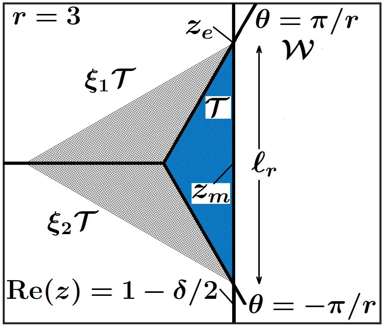
The set $\mathcal{T}$ (darker shaded region) in relation to $\mathcal{W}$, for $r=3$. The rotated sets $\xi_{j}\mathcal{T}$ (lighter shaded regions) satisfy the constraint inequality in equation (4.9), $\mathrm{Re}(\xi_{j}\mathcal{T})<1-\delta/2$. The set $\mathcal{D}_{-\infty}$ is given by $\mathcal{D}_{-\infty}=\varphi^{-1}(\mathcal{T})$.

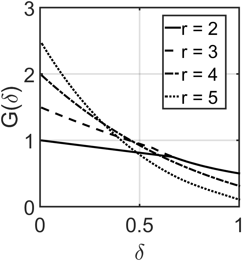
Figure 1: Left: the set $\mathcal{T}$.  Right: plot of $G(\delta)$, as defined by equation (4.12).

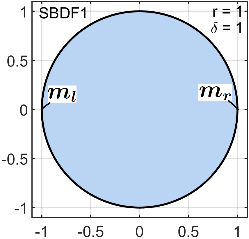
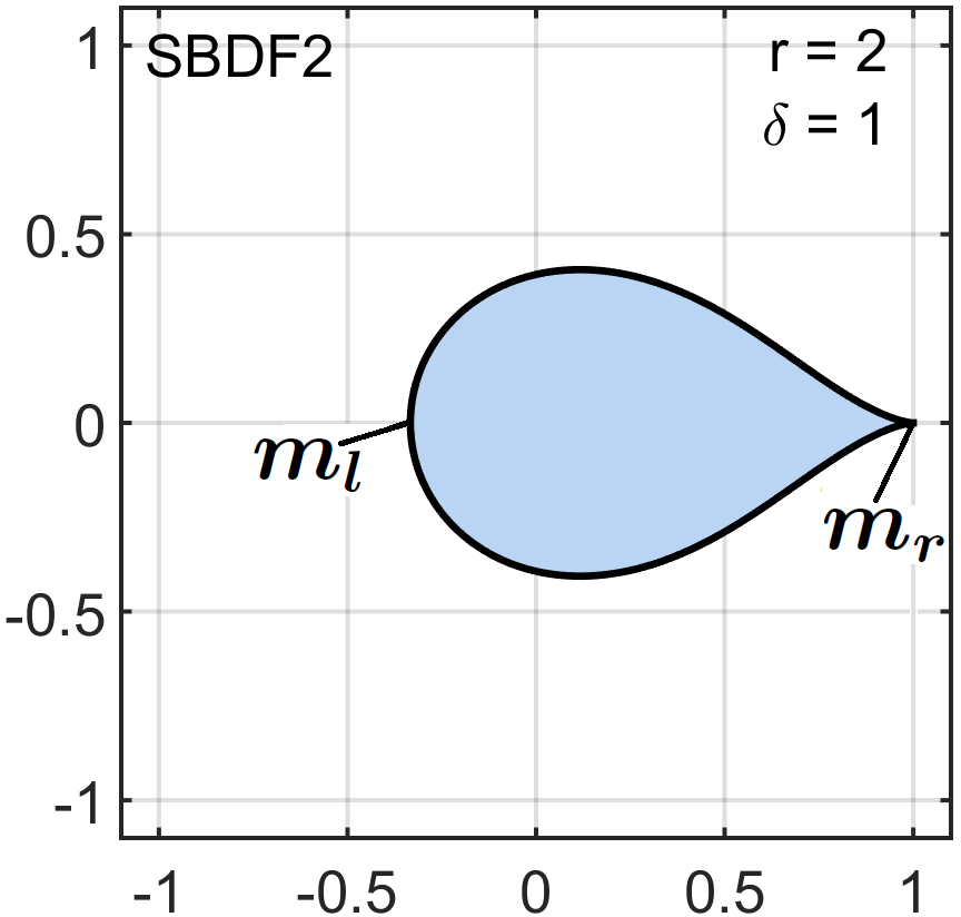
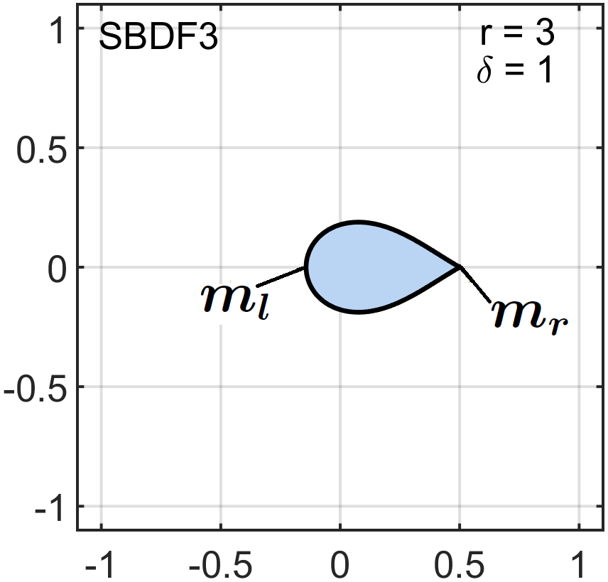
Figure 2: The sets $\mathcal{D}_{-\infty}$ (which by virtue of Proposition 4.4 equal $\mathcal{D}$) are shown shaded. The parameters are: $\delta=1$ (SBDF schemes) and orders $r=1,2,3$ (left to right). Formulas for the boundary are given by Theorem 4.3.

Figure 2 illustrates Theorem 4.3 by plotting the sets $\mathcal{D}_{-\infty}$ for the well-known SBDF schemes. Using the characterization of $\mathcal{D}_{-\infty}$ in Theorem 4.3, we are now in a position to show that not only is $\mathcal{D}\subseteq\mathcal{D}_{-\infty}$, but that this inclusion is also an equality: $\mathcal{D}=\mathcal{D}_{-\infty}$.

To first illustrate that $\mathcal{D}=\mathcal{D}_{-\infty}$, in Figure 3 we plot $\mathcal{D}_{y}$ for different values of $y$, using the boundary locus (chapter 7.6, [39]) method. Specifically, $\mathcal{D}_{y}$ is a region whose boundary is a subset of the locus

$$\varGamma_{y}:=\Big{\{}\frac{1}{b(z)}\big{(}c(z)-y^{-1}a(z)\big{)}:|z|=1\Big{\}},\quad\varGamma_{-\infty}:=\Big{\{}\frac{c(z)}{b(z)}:|z|=1\Big{\}}.$$ (4.11)

Equation (4.11) is obtained by isolating $\mu$ in equation (3.6) and letting $z$ vary over the unit circle. Figure 3 shows the nested stability regions $\mathcal{D}_{y}$ for orders $r=3,4,5$ and fixed parameter value $\delta=1$. In the figure, the solid curve traces out $\varGamma_{y}$ corresponding to the boundary locus for $\mathcal{D}_{y}$. The dashed curves show as a reference $\varGamma_{y}$ for different $y$ values. Although the plots are only for one value of $\delta$, the limiting behavior $\mathcal{D}=\mathcal{D}_{-\infty}$ is observed for all $0<\delta\leq 1$.

We now show that the set equality $\mathcal{D}=\mathcal{D}_{-\infty}$ is a direct consequence of the fact that the function $G(\delta)$ (defined below for the ImEx schemes in Definition 4.1) is positive. Note that $G(\delta)$, roughly speaking, is a measure of the distance of $\varGamma_{y}$ to the set $\mathcal{D}_{-\infty}$ — and it is the key to showing that $\mathcal{D}=\mathcal{D}_{-\infty}$.

$$G(\delta):=\inf_{y<0}\min_{w\in\varGamma_{y}}\Big{[}\Big{(}\mathrm{Re}\big{(}\varphi(w)\big{)}-(1-\delta/2)\Big{)}(1-y)\delta^{-2}\Big{]}.$$ (4.12)

This function may be numerically computed, which leads to:

Numerical observation 1.

Numerical computations (shown in Figure 1, right) indicate that: for $0<\delta\leq 1$ and $2\leq r\leq 5$, $G(\delta)>0$.

This fact is introduced as an assumption below, in Proposition 4.4.

The positive factor $(1-y)\delta^{-2}$ in equation (4.12) is included to re-scale the difference between $\mathrm{Re}(\varphi(w))$ and $(1-\delta/2)$, which vanishes as $y\rightarrow-\infty$ or $\delta\rightarrow 0$. This re-scaling helps to visually verify that $G(\delta)$ does not change sign, even as $y\rightarrow-\infty$ or $\delta\rightarrow 0$. To computationally handle the infinite interval $-\infty<y<0$, we introduce the change of variables $\tilde{y}=(1-y)^{-1}$, so that $0<\tilde{y}<1$. For each fixed value of $\tilde{y}$, we parameterize $\varGamma_{y}$ as the image of the unit circle, which then allows us to compute $G(\delta)$ as a double minimization over two real variables on bounded intervals.

Proposition 4.4.

(The set $\mathcal{D}=\mathcal{D}_{-\infty}$) (i) For $r=1$ and $0<\delta\leq 1$, $\mathcal{D}=\mathcal{D}_{-\infty}$. (ii) For $2\leq r\leq 5$, assume that: $G(\delta)>0$, $0<\delta\leq 1$. Then

$$\mu\in\mathcal{D}_{-\infty}\quad\Longrightarrow\quad\mu\in\mathcal{D}_{y}\textrm{ for any }y\in\mathbb{R}_{<0}.$$ (4.13)

In other words, for every $y\in\mathbb{R}_{<0}$ the set $\mathcal{D}_{y}$ contains the limiting set $\mathcal{D}_{-\infty}$. As a result, the unconditional stability region is $\mathcal{D}=\mathcal{D}_{-\infty}$.

Proof.

(Proposition 4.4) For (i), the proof is straightforward as $\mathcal{D}_{y}$ is a disk centered at $1-(\delta^{-1}-y^{-1})$ with radius $\delta^{-1}-y^{-1}$. For (ii) the proof involves two steps. First, we use a standard continuity argument to show that if $\mu\in\mathcal{D}_{-\infty}$, but $\mu\notin\mathcal{D}_{y_{0}}$ for some $y_{0}<0$, then there is an intermediate $y$-value ($-\infty<y<y_{0}$) where $\mu$ must lie on the boundary locus $\mu\in\varGamma_{y}$. Next we show that $\varGamma_{y}$ is bounded away from $\mathcal{D}_{-\infty}$ when $y<0$. It then follows that $\mu\in\mathcal{D}_{y}$ whenever $\mu\in\mathcal{D}_{-\infty}$.

To proceed with the first step, we define the following polynomial function based on equation (3.6)

$$P(z;\tilde{y}):=c(z)-\mu b(z)+\frac{\tilde{y}}{1-\tilde{y}}a(z).$$ (4.14)

Here $y=1-\tilde{y}^{-1}$, so that $0<\tilde{y}<1$ (resp. $\tilde{y}=0$) corresponds to $y<0$ (resp. $y=-\infty$), which will be useful in the subsequent continuity argument. To minimize additional notation, we will continue to use $\mathcal{D}_{y}$ and $\varGamma_{y}$ as sets, and $\tilde{y}$ as the parameter in the polynomials, with the understanding that $y=1-\tilde{y}^{-1}$. Then $\mathcal{D}_{y}$ is defined as $\mu\in\mathbb{C}$ such that $P(z;\tilde{y})$ has $r$ roots inside the unit circle, or alternatively: (i) $P(z;\tilde{y})\neq 0$ on the unit circle $|z|=1$, and (ii) the function $F(\tilde{y})=r$, where $F(\tilde{y})$ counts the number of roots $|z|<1$ via the Cauchy integral formula:

$$F(\tilde{y}):=\frac{1}{2\pi\imath}\oint_{|z|=1}\frac{P_{z}(z;\tilde{y})}{P(z;\tilde{y})}\,\mathrm{d}z.$$

Now, $F(\tilde{y})$ is continuous as a function of $\tilde{y}$, and also a constant, as long as it is defined. The only way $F(\tilde{y})$ may change values is if $P(z;\tilde{y})=0$ vanishes for some $|z|=1$ on the unit circle, which implies $\mu\in\varGamma_{y}$. Hence, if for a given $\mu$, $F(0)=r$ and $F(\tilde{y}_{0})\neq r$, then there must exist a point $0<\tilde{y}<\tilde{y}_{0}$ such that $\mu\in\varGamma_{y}$.

To show that $\varGamma_{y}$ does not intersect $\mathcal{D}_{-\infty}$ for $0<\tilde{y}<1$, we exploit the fact that the mapping $\varphi(z)$, defined in Theorem 4.3, simplifies the shape of $\varphi(\mathcal{D}_{-\infty})=\mathcal{T}$. Specifically, $\varphi(z)$ is a one-to-one mapping of $\mathbb{C}$ to the wedge $\mathcal{W}$, so that it is sufficient to show that the mappings of $\mathcal{D}_{-\infty}$ and $\varGamma_{y}$ under $\varphi(z)$ do not intersect, i.e. $\varphi(\varGamma_{y})$ does not intersect $\mathcal{T}$, for $0<\tilde{y}<1$. Since $\mathcal{T}$ is contained within the half-plane $\mathrm{Re}(z)<1-\delta/2$, we arrive at the following observation: if

$$\mathrm{Re}\big{(}\varphi(w)\big{)}-(1-\delta/2)>0,\quad\textrm{for all }0<\tilde{y}<1,\;w\in\varGamma_{y},$$ (4.15)

then $\varphi(\varGamma_{y})$ and $\mathcal{T}$ do not intersect. Multiplying the left-hand side of the inequality (4.15) by the positive factor $\delta^{-2}\tilde{y}^{-1}=\delta^{-2}(1-y)>0$, and minimizing over $0<\tilde{y}<1,\;w\in\varGamma_{y}$, yields the function $G(\delta)$. Hence, we arrive at the conclusion that $\varphi(\varGamma_{y})$ and $\mathcal{T}$ do not intersect whenever $G(\delta)>0$, which together with the first step of the proof, implies $D_{-\infty}\subseteq\mathcal{D}_{y}$ for all $y<0$. ∎

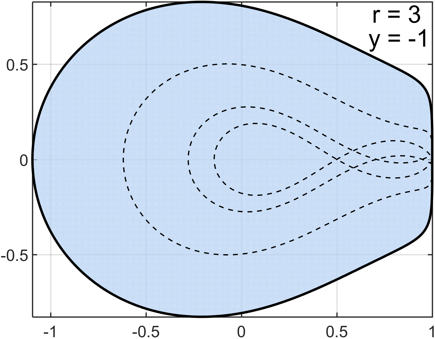
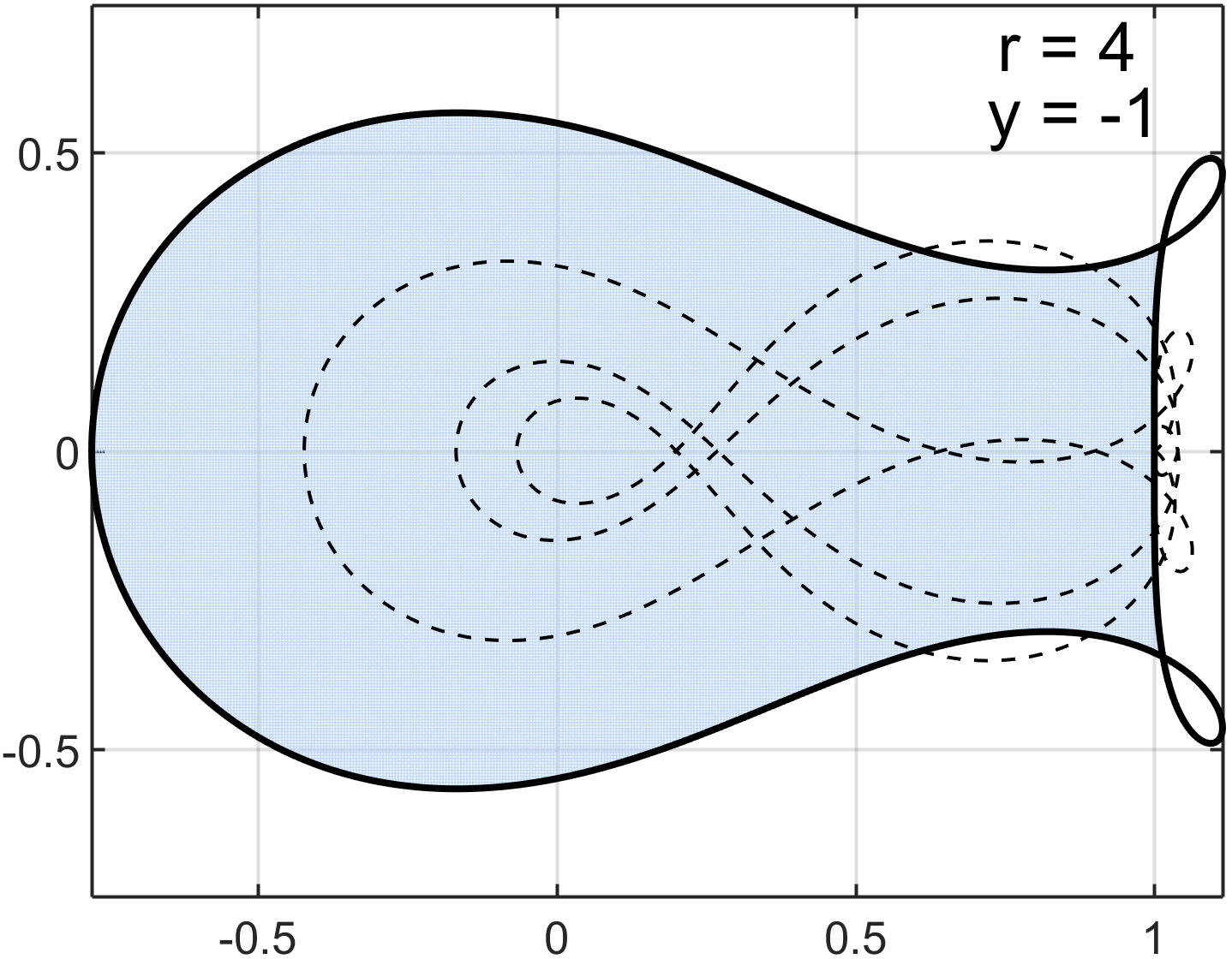
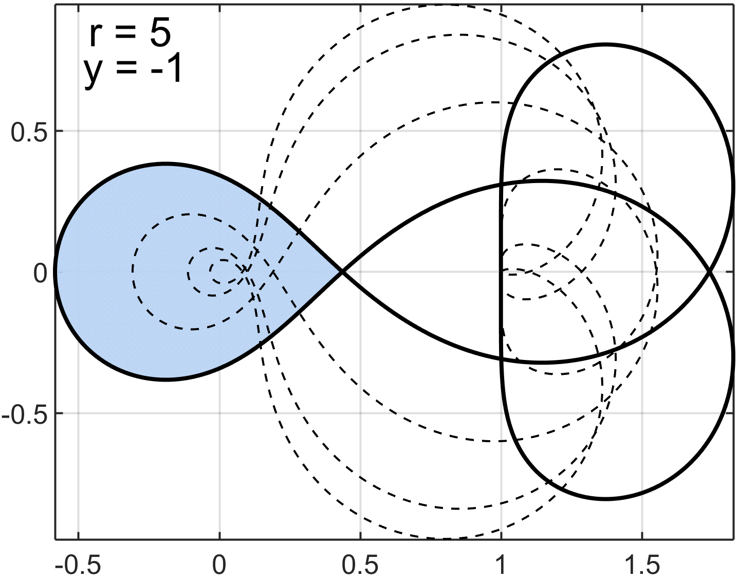
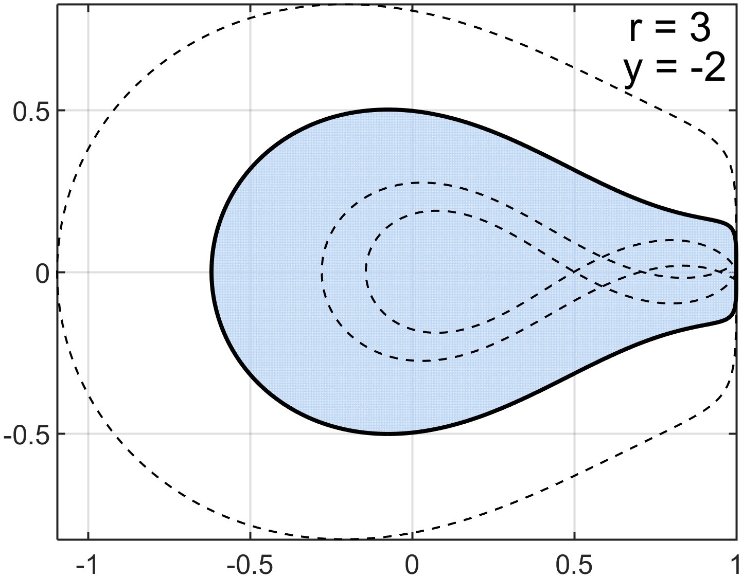
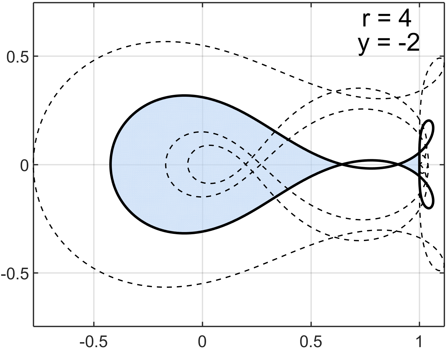
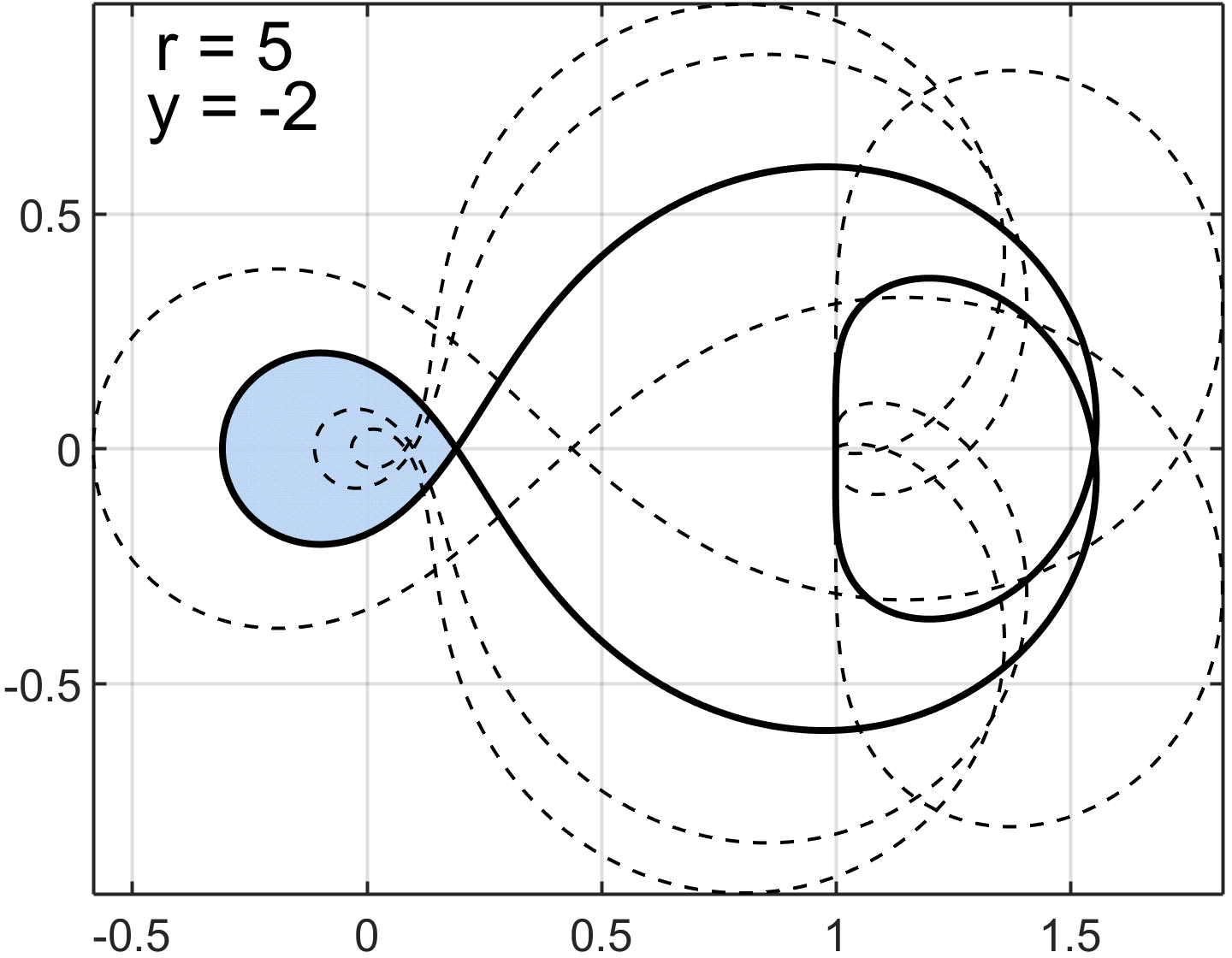
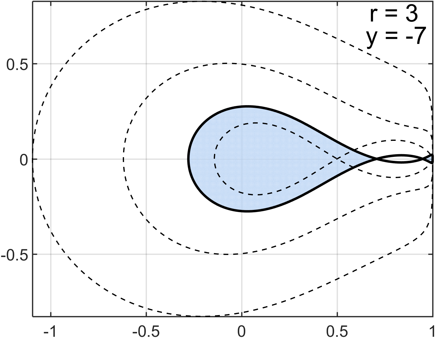
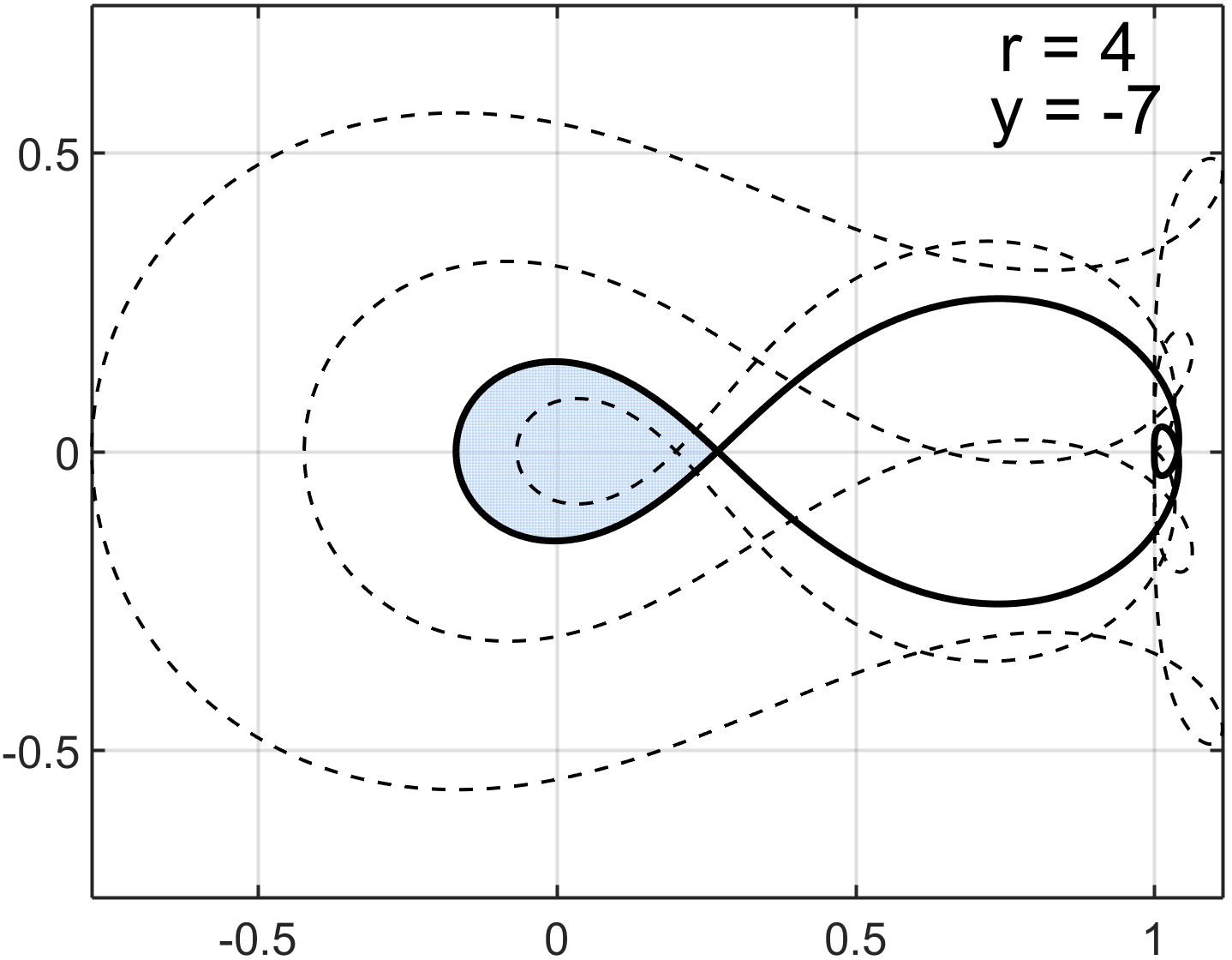
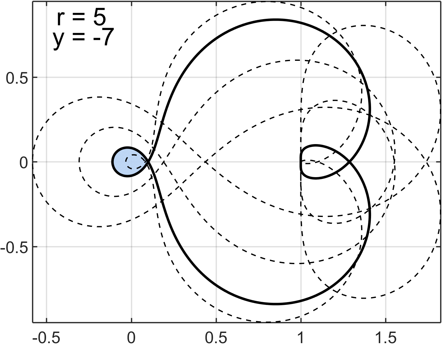
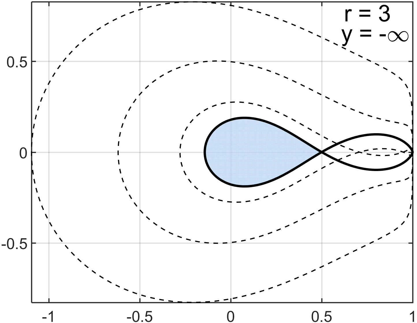
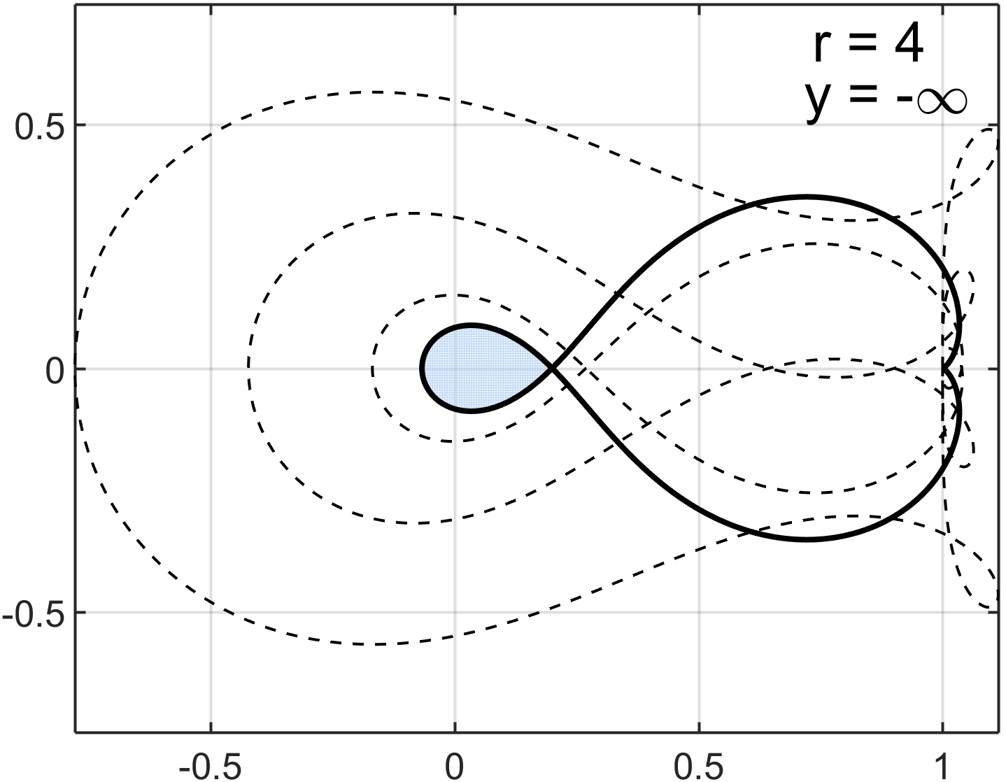
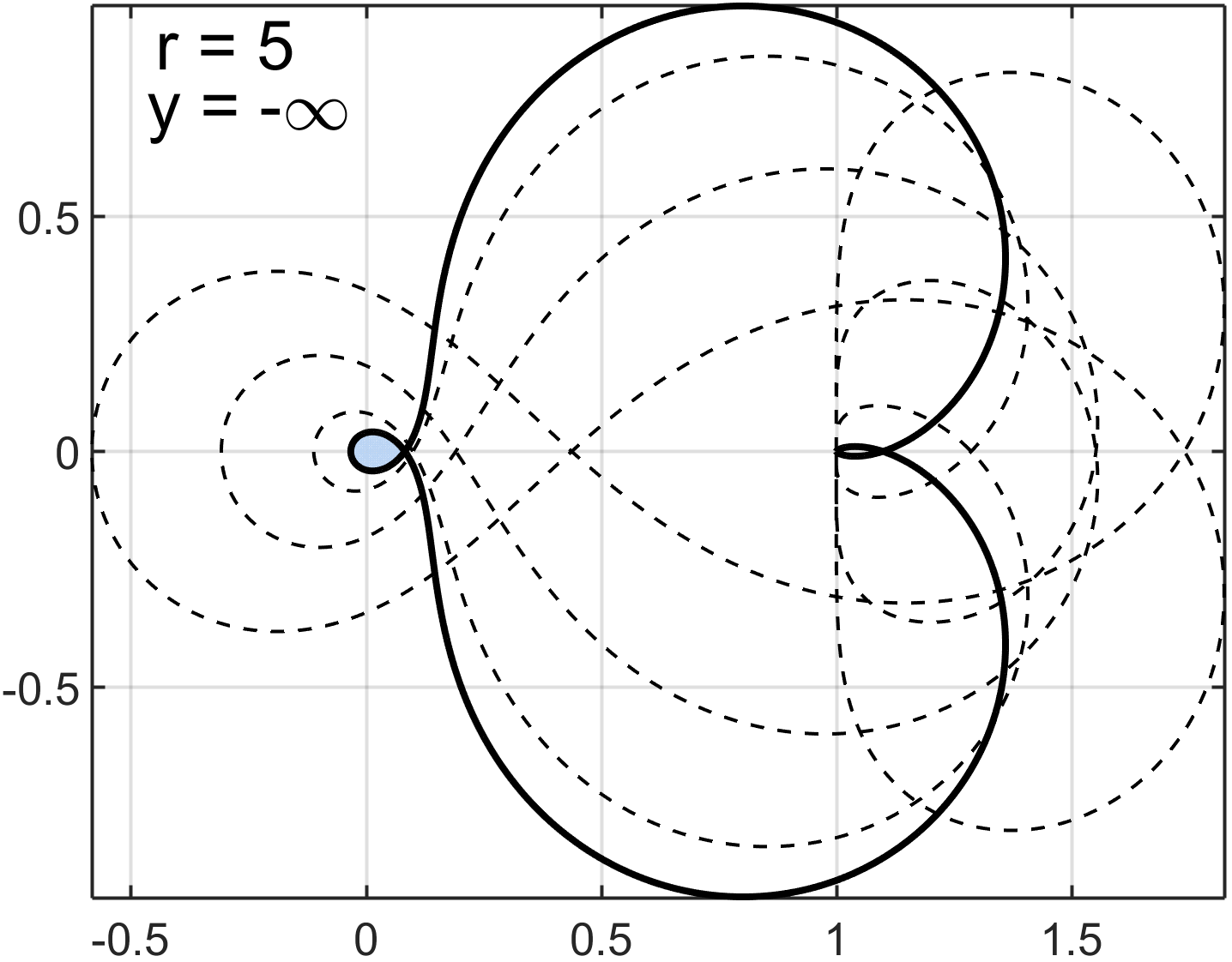
Figure 3: Visualization of Proposition 4.4: $\mathcal{D}_{-\infty}$ is contained in $\mathcal{D}_{y}$ for all $y<0$. Plot of the boundary locus $\varGamma_{y}$ (black curves) and the stability regions $\mathcal{D}_{y}$ (shaded regions) for: $y=-1,-2,-7,-\infty$ (top to bottom), orders $r=3,4,5$ (left to right), and fixed parameter value $\delta=1$. In each plot, the dashed lines $\varGamma_{-1},\varGamma_{-2},\varGamma_{-7},\varGamma_{-\infty}$ are shown for reference. Note that the inclusion $\mathcal{D}_{-\infty}\subseteq\mathcal{D}_{y}$ is valid for all $y\in\mathbb{R}_{<0}$.

With the exact boundary locus description in Theorem 4.3, and the subsequent result that $\mathcal{D}=\mathcal{D}_{-\infty}$, one may provide an asymptotic description of $\mathcal{D}$ in the limit $\delta\ll 1$.

Remark 4.

(Asymptotic $\mathcal{D}$) Define the circle $C$ as

$$C =\Big{\{}z\in\mathbb{C}:\Big{|}z+\frac{1}{r\delta}-\frac{r+1}{2r}\Big{|}\leq\frac{1}{r\delta}\Big{\}}.$$

Taking the asymptotic limit $\delta\ll 1$ and values of $|z-1|\gg\delta$ in formula (4.4) for $\partial\mathcal{D}$ (which correspond to points in $\mathcal{D}$ away from the right-most values along the real axis), the exact boundary $\partial\mathcal{D}$ approaches the circle $\partial C$: $\mathcal{D}\approx C+\mathcal{O}(\delta).$ For $r=1$, the domain $\mathcal{D}=C$ is a circle for all $0<\delta\leq 1$.

The circle $C$ in Remark 4 is obtained via an asymptotic computation, i.e. $\delta\rightarrow 0$, of (4.4). Specifically, note that the starting value of the locus description for $\mathcal{D}_{-\infty}$ in Theorem 4.3 satisfies $|z_{0}-1|=\mathcal{O}(\delta)$, so that the locus parameter $z$ almost traces through an entire circle. Consider points $|z-1|\gg\delta$ and expand $c(z)/b(z)$ in a Laurent series in powers of $\delta$ about $z=1$:

$$\frac{c(z)}{b(z)} =\frac{(z-1)^{r}+\delta r(z-1)^{r-1}+\dotsb}{\delta r(z-1)^{r-1}+\delta^{2}\frac{r(r-1)}{2}(z-1)^{r-2}+\dotsb}$$

$$=\frac{1}{\delta r}\Big{(}\frac{(z-1)+\delta r+\mathcal{O}(\delta^{2})}{1+\delta\frac{(r-1)}{2}(z-1)^{-1}+\mathcal{O}(\delta^{2})}\Big{)}=\frac{1}{r\delta}(z-1)+\frac{r+1}{2r}+\mathcal{O}(\delta).$$ (4.16)

For values $|z|=1$, equation (4.16) describes the boundary of the circle $C$ defined in Remark 4 with radius $\frac{1}{r\delta}$ and center $\frac{r+1}{2r}-\frac{1}{r\delta}$. Hence $\partial\mathcal{D}\approx\frac{1}{r\delta}(z-1)+\frac{r+1}{2r}+\mathcal{O}(\delta)$, for $|z-1|\gg\mathcal{O}(\delta)$. Figure 4 shows the regions $\mathcal{D}$ for different parameter values $\delta$ and orders $2\leq r\leq 5$. In particular, the figure illustrates how the regions $\mathcal{D}$ grow larger with decreasing $\delta$ values, and also approach the asymptotic circle $C$.

Having precise estimates for the geometric properties of $\mathcal{D}$, such as the formulas for $m_{r}$, $m_{l}$ and $C$, is very useful for the design of unconditionally stable schemes. Specifically the design of an unconditionally stable scheme require a simultaneous choice of matrix splitting $(\mbox{\boldmath$A$},\;\mbox{\boldmath$B$})$, and time stepping coefficients $(a_{j},b_{j},c_{j})$. If one knows, either through direct numerical computation or analytic estimates, $W_{p}$ for a matrix splitting $(\mbox{\boldmath$A$},\;\mbox{\boldmath$B$})$, then the estimates for $m_{r},m_{l}$ and $C$ can be used to choose a $\delta$ value large enough to guarantee that $W_{p}\subseteq\mathcal{D}$. Such a choice of $\delta$ will then provide the suitable time stepping coefficients that guarantee unconditional stability. We highlight such an approach in several numerical examples in §5, as well as in greater detail in a companion paper on the practical aspects of unconditional stability for multistep ImEx schemes.

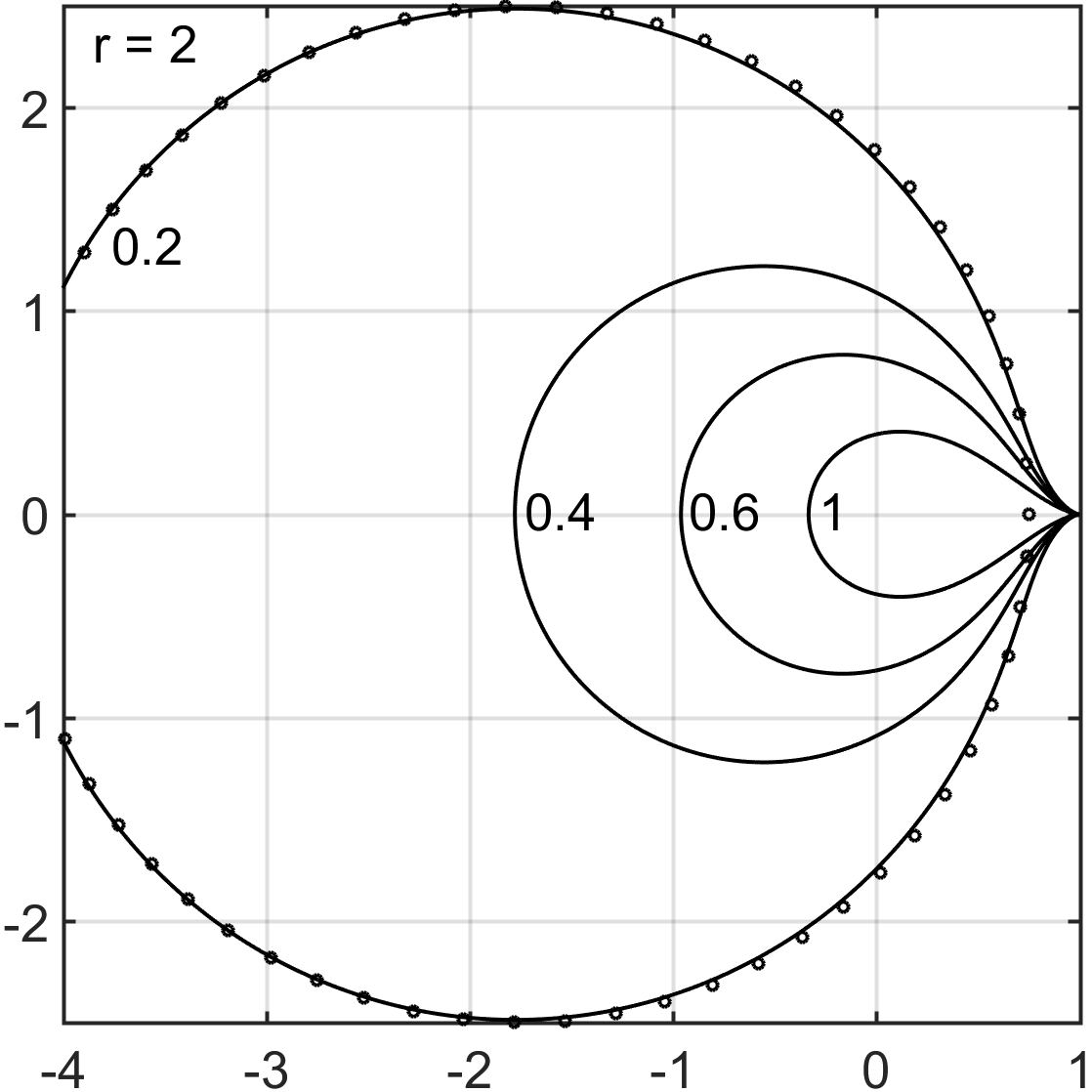
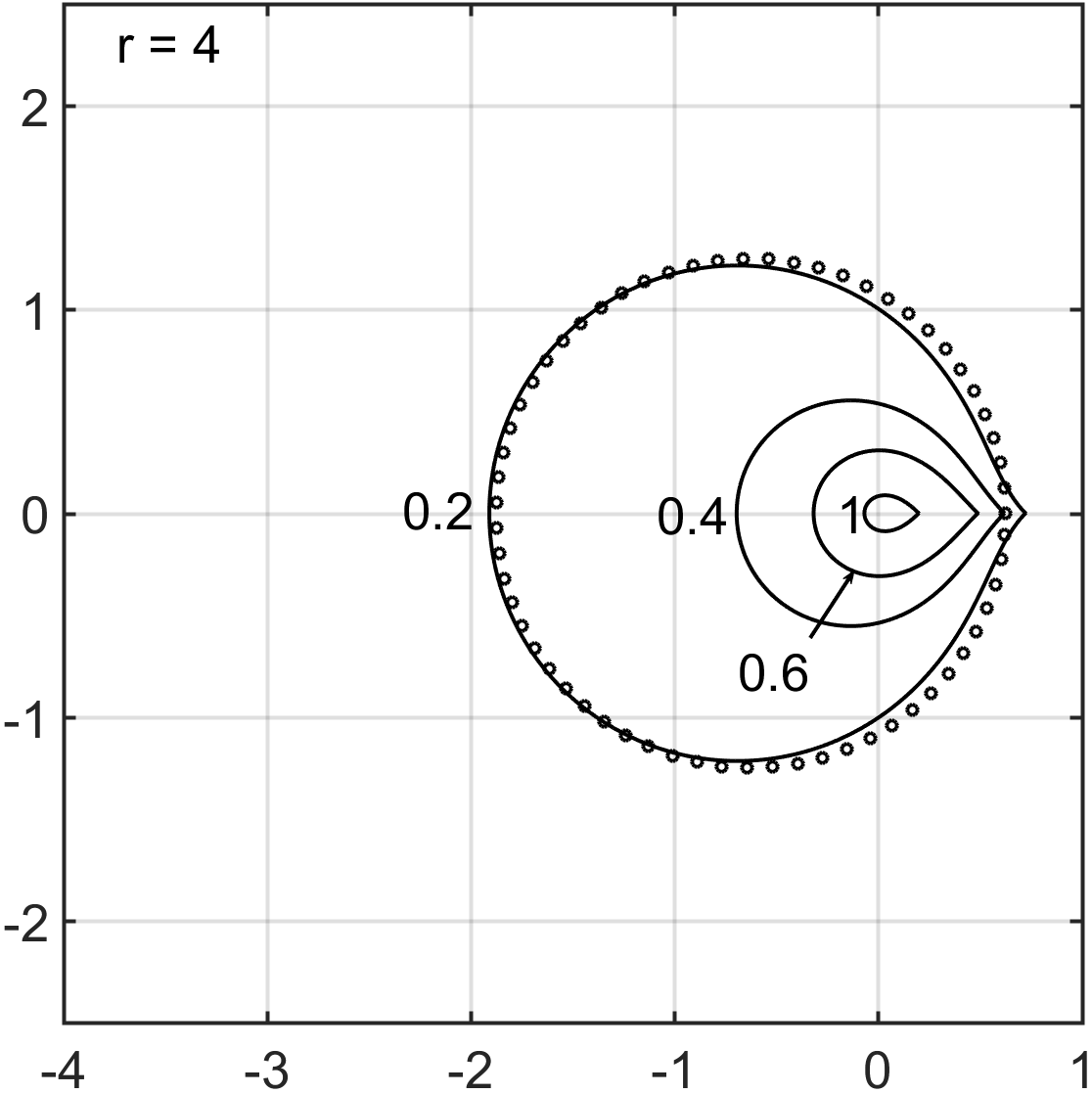
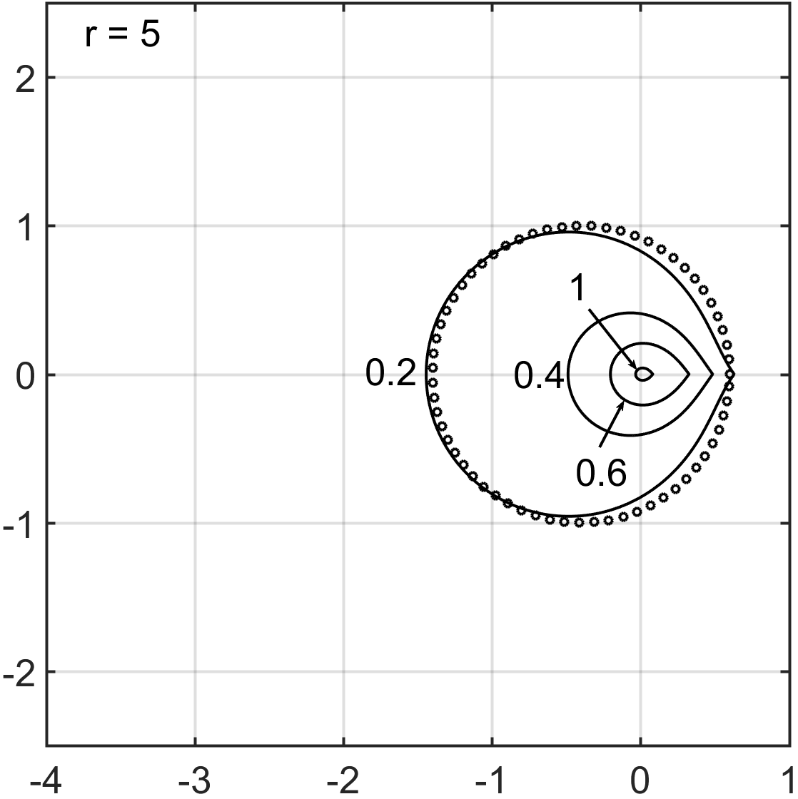
Figure 4: Region of unconditional stability $\mathcal{D}$ for orders $r=2,3,4,5$. In each sub-figure, the boundary $\partial\mathcal{D}$ (solid line) is shown for parameter values $\delta=0.2,0.4,0.6,1$ ($\delta=1$ corresponds to SBDF).
For small $\delta\ll 1$, the stability region becomes arbitrarily large. With the exception of points near the positive real axis, it approaches the asymptotic circle $C$ defined in Theorem 4.3. The dots ($\circ$) show $C$ for $\delta=0.2$.

4.3 Necessary conditions for unconditional stability

The sufficient conditions for unconditional stability $W_{p}\subseteq\mathcal{D}$, are not sharp, and we supplement them with additional necessary conditions. Let

$$\sigma((-\mbox{\boldmath$A$})^{-1}\mbox{\boldmath$B$})=\{\mu\in\mathbb{C}:\mu(-\mbox{\boldmath$A$})\mbox{\boldmath$u$}=\mbox{\boldmath$B$}\mbox{\boldmath$u$},\mbox{\boldmath$u$}\neq\mbox{\boldmath$0$}\}$$

be the generalized eigenvalues of $(-\mbox{\boldmath$A$}),\mbox{\boldmath$B$}$.

Proposition 4.5.

(Necessary condition for unconditional stability) Given a set of ImEx time stepping coefficients (Definition 4.1), and the corresponding stability diagram $\mathcal{D}$, then a necessary condition for unconditional stability of the scheme in (2.1), is that the eigenvalues satisfy $\sigma((-\mbox{\boldmath$A$})^{-1}\mbox{\boldmath$B$})\subseteq\mathcal{D}\cup\varGamma_{-\infty}$.

Proof.

The idea behind the necessary condition is that in the limit of large time steps $k\rightarrow\infty$, the nonlinear eigenvalue problem (3.4) governing stability, can be solved using the eigenvectors of the matrix $(-\mbox{\boldmath$A$})^{-1}\mbox{\boldmath$B$}$. As a result, a necessary condition for unconditional stability may be placed on the eigenvalue spectrum $\mu\in\sigma((-\mbox{\boldmath$A$})^{-1}\mbox{\boldmath$B$})$.

We first prove a slightly stronger statement. Let

$$\mathcal{A}:=\{\mu\in\mathbb{C}:(\ref{Simplified_Polynomial})\textrm{ has a solution }|z|>1\}.$$

Then $\sigma((-\mbox{\boldmath$A$})^{-1}\mbox{\boldmath$B$})\subseteq\mathcal{A}^{c}$ is a necessary condition for unconditionally stability. This is because, in the limit $k\rightarrow\infty$, the nonlinear eigenvalue problem (3.4) becomes

$$\mbox{\boldmath$T$}(z)\mbox{\boldmath$u$}=-c(z)\mbox{\boldmath$A$}\mbox{\boldmath$u$}-b(z)\mbox{\boldmath$B$}\mbox{\boldmath$u$}=0.$$ (4.17)

Hence, an eigenvector $\mbox{\boldmath$u$}_{\mu}$ to $(-\mbox{\boldmath$A$})^{-1}\mbox{\boldmath$B$}$ with eigenvalue $\mu\in\sigma((-\mbox{\boldmath$A$})^{-1}\mbox{\boldmath$B$})$ becomes an eigenvector of (4.17)

$$\mbox{\boldmath$T$}(z)\mbox{\boldmath$u$}_{\mu}=-(c(z)-\mu b(z))\mbox{\boldmath$A$}\mbox{\boldmath$u$}_{\mu}=0.$$ (4.18)

Thus the eigenvalues $z$ satisfy (4.6), since $\mbox{\boldmath$A$}\mbox{\boldmath$u$}_{\mu}\neq 0$ because $A$ is invertible. If $\mu$ is also in $\mathcal{A}$, then at least one solution to (4.18) satisfies $|z|>1$. Finally, we note that any nonlinear eigenvalue $|z|>1$, arising in the limit $k\rightarrow\infty$, will yield a slightly perturbed eigenvalue when $0<k^{-1}\ll 1$. Thus, for any $k$ sufficiently large (but finite) an unstable eigenvalue satisfying $|z|>1\/$ will exist.

Finally we observe that $\mathcal{A}^{c}\subseteq\mathcal{D}\cup\varGamma_{-\infty}$. The reason is that every $\mu\in\mathcal{A}^{c}$ has one of the following properties: (i) all solutions to (4.6) have $|z|<1$, implying $\mu\in\mathcal{D}$, or (ii) at least one solution to (4.6) has $|z|=1$ (with all the others $|z|<1$), implying $\mu\in\varGamma_{-\infty}$. ∎

Remark 5.

Numerical experiments (such as the diagrams in Figure 3) suggest that the set $\mathcal{D}\cup\varGamma_{-\infty}$ in Proposition 4.5 can be further reduced to include only the portion of $\varGamma_{-\infty}$ that is the boundary $\partial\mathcal{D}$ and the single point $\{1\}$.

Remark 6.

In the limit $\delta\rightarrow 0$, $\mathcal{D}$ approaches the circle $C$ which encompasses an entire complex half-plane:

$$\Big{\{}\mu\in\mathbb{C}:\mathrm{Re}(\mu)<\frac{r+1}{2r},1\leq r\leq 5\Big{\}}\subseteq\lim_{\delta\rightarrow 0}\mathcal{D}.$$ (4.19)

The limiting $\mathcal{D}$ also contains the real half-line $(-\infty,(1+\cos^{r}(\pi/r))^{-1})$, for $2\leq r\leq 5$.

4.4 Numerical error dependence on $\delta$ for the new ImEx coefficients

Up to now, the results appear to indicate that one should choose $\delta\ll 1$ (extremely small) to yield a large unconditional stability region. In this section we describe why this is not a good strategy. In particular, we investigate the dependence of the global truncation error (GTE) on $\delta$ for the new ImEx coefficients. We do so by running numerical tests, and computing the error constants which characterize the leading order asymptotic GTE behavior in $k$.

The GTE at time $t_{n}=nk$, is defined by $\|\mbox{\boldmath$u$}_{n}-\mbox{\boldmath$u$}^{*}(nk)\|_{\ell^{\infty}}$ and depends on $L$, the time stepping coefficients, and the forcing $\mbox{\boldmath$f$}(t)$. Here $\mbox{\boldmath$u$}^{*}(t)$ is the exact ODE solution to (1.1) at time $t$. Formally, the new ImEx schemes given in Definition 4.1 achieve $r$-th order accuracy, so that the $\textrm{GTE}=\mathcal{O}(k^{r})$. The leading order constant in the GTE depends on $\mbox{\boldmath$A$},\mbox{\boldmath$B$},\mbox{\boldmath$f$}$ and the time stepping coefficients (for error constants in an LMM see equation (2.3), p. 373, in [26]). In ImEx schemes one may examine two separate error constants, an implicit $C_{I,r}$ (resp. explicit $C_{E,r}$) constant characterizing the error of a purely implicit (resp. explicit) scheme where $\mbox{\boldmath$B$}=0$ (resp. $\mbox{\boldmath$A$}=0$):

$$C_{I,r}:=\frac{R_{I,r}}{c(1)}=\delta^{-r}R_{I,r},\quad\quad C_{E,r}:=\frac{R_{E,r}}{b(1)}=\delta^{-r}R_{E,r}.$$ (4.20)

Here we have used the fact that $c(1)=b(1)=\delta^{r}$ for the new ImEx schemes, while the constants $R_{I,r},R_{E,r}$ quantify how much the $r$-th order coefficients (when $r=s$) fail to satisfy the $(r+1)th$ order conditions (B.1)

$$R_{I,r}=\frac{1}{(r+1)!}\sum_{j=0}^{r}\Big{(}a_{j}j^{r+1}-(r+1)c_{j}j^{r}\Big{)},\hskip 5.69054ptR_{E,r}=\frac{1}{(r+1)!}\sum_{j=0}^{r}\Big{(}a_{j}j^{r+1}-(r+1)b_{j}j^{r}\Big{)}.$$

Even though $R_{I,r},R_{E,r}$ depend on $\delta$, both constants satisfy $R_{I,r}=\mathcal{O}(1),R_{E,r}=\mathcal{O}(1)$, for all values of $0<\delta\leq 1$. As a result, the asymptotic $\delta\ll 1$ behavior on the GTE for the new ImEx coefficients is $\textrm{GTE}=\mathcal{O}(\delta^{-r}k^{r})$. The numerical tests in §5, as well as those in §C, confirm the estimate GTE $\sim\delta^{-r}k^{r}$. As a result of this scaling, we adopt the general philosophy: given a splitting $(\mbox{\boldmath$A$}\/,\,\mbox{\boldmath$B$})$, choose $\delta$ as large as possible while maintaining unconditional stability.

5 Two illustrative examples

In this section we highlight the potential of the new ImEx coefficients to obtain unconditionally stable schemes. The first example (§5.1) illustrates that a small implicit term can stabilize a larger explicit term. The second example (§5.2) represents the numerical discretization of a variable coefficient diffusion equation. For this stiff problem, unconditional stability for orders $r>2$ is beyond the capabilities of classical SBDF schemes; however, the new coefficients achieve the goal.

5.1 A single variable ODE

Consider the ODE

$$u_{t}=-10u=-u-9u,$$ (5.1)

with splitting $\mbox{\boldmath$A$}u:=-u$ and $\mbox{\boldmath$B$}u:=-9u$. For this simple case, $(\mbox{\boldmath$A$},\mbox{\boldmath$B$})$ are numbers, or $1\times 1$ matrices. An important observation is that $|\mbox{\boldmath$A$}|=1$, while $|\mbox{\boldmath$B$}|=9$, i.e., the implicit term is 9 times smaller than the explicit term.

The set $W_{1}=\{-9\}$ consists of one element, and it is also equal to the generalized eigenvalue $\sigma((-\mbox{\boldmath$A$})^{-1}\mbox{\boldmath$B$})=\{-9\}$. Therefore unconditional stability requires that $\{-9\}\subseteq\mathcal{D}$. Using the fact that the left-most endpoint of $\mathcal{D}$ is given by $m_{l}$ in formula in Remark 4.3, one obtains unconditional stability for an $r$-th order scheme, provided that

$$\frac{-(2-\delta)^{r}}{2^{r}-(2-\delta)^{r}}<-9,\quad\Longleftrightarrow\quad\delta<2\Big{[}1-\big{(}\frac{9}{10}\big{)}^{1/r}\Big{]}.$$

Note that for a fixed $\delta$ value, the unconditional stability regions $\mathcal{D}$ become smaller with increasing $r$. Setting $r=5$ inside the inequality yields $\delta<0.0417$. Therefore, a choice of the parameter value $\delta=0.04$ inside the new ImEx coefficients guarantees that $W_{1}\subseteq\mathcal{D}$ for $r=5$, and hence subsequently for all $1\leq r\leq 5$. Hence, the smaller implicit term stabilizes the instabilities generated by the explicit term, thus achieving unconditional stability.

5.2 A PDE example: variable coefficient diffusion

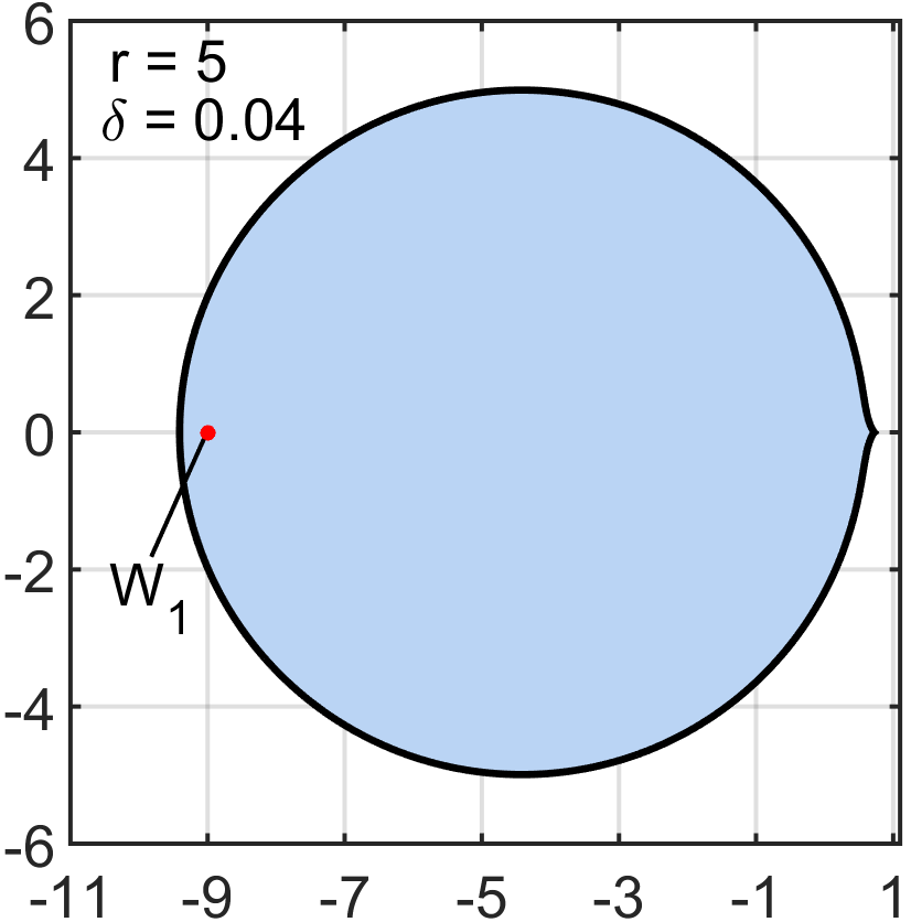
Figure 5: ODE example (5.1). Note that $W_{1}$ (red $\circ$) is contained in $\mathcal{D}$ (shaded region) for the parameter value $\delta=0.04$ and order $r=5$. Using the new ImEx coefficients with $\delta=0.04$ yields an unconditionally stable scheme.

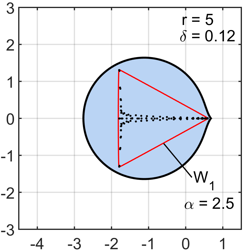
Figure 6: PDE example for variable diffusion coefficient problem. The stability diagram $\mathcal{D}$ (shaded region) is for the parameter $\delta=0.12$ and order $r=5$, and contains $W_{1}$ (red curve shows the boundary). The black dots show the generalized eigenvalues $\sigma((-\mbox{\boldmath$A$})^{-1}\mbox{\boldmath$B$})$.

This example demonstrates how one might use the new ImEx coefficients, in conjunction with the sufficient conditions for unconditional stability, to avoid a stiff time step restriction in the spatial discretization of a PDE. Specifically, we numerically solve the variable coefficient diffusion equation on the domain $\varOmega=(-1,1)$:

$$u_{t}=\big{(}d(x)u_{x}\big{)}_{x}+f(x,t),\quad\quad\textrm{on }\varOmega\times(0,T],$$

with Dirichlet boundary conditions, $u=0$, on $x\in\{-1,1\}$. Here $d(x)>0$ is a spatially dependent diffusion coefficient.

For the spatial discretization, we adopt a Chebyshev spectral method (chapter 5–7, [47]) using the $N+2$ Chebyshev collocation points

$$x_{j}=\cos\Big{(}\frac{j\pi}{N+1}\Big{)},\quad 0\leq j\leq N+1,\quad\textrm{with }\quad\mbox{\boldmath$u$}=\begin{pmatrix}u(x_{1}),\ldots,u(x_{N})\end{pmatrix}^{T}\in\mathbb{R}^{N}.$$

We also use the boundary conditions to set $u(x_{0})=u(x_{N+1})=0$ so that there are only $N$ independent variables. Let $\mbox{\boldmath$D$}_{N}$ be the spectral differentiation matrix, so that $\mbox{\boldmath$D$}_{N}\mbox{\boldmath$u$}\approx u_{x}(x)$. The matrix $L$ is then built using the Dirichlet boundary conditions by constructing

$$\mbox{\boldmath$L$}=\mbox{\boldmath$D$}_{N}\;\textrm{diag}\big{(}d(x_{j})\big{)}\;\mbox{\boldmath$D$}_{N}.$$

Here $L$ acts on $u$ at the $N$ grid points $x_{1},x_{2},\ldots,x_{N}$ (see page 62, chapter 7 in [47] for details). Note that due to collocation of the boundary conditions, the matrix $L$, as well as the Laplacian $(\mbox{\boldmath$D$}_{N})^{2}$, are not symmetric. However, the spectrum of $L$ and $\mbox{\boldmath$D$}_{N}^{2}$ are still purely real, in contrast with the situation in truly asymmetric problems, such as advection-diffusion.

In practice, the semi-implicit time stepping of (2.1), using the schemes defined by Definition 4.1, requires both a choice of splitting $(\mbox{\boldmath$A$},\mbox{\boldmath$B$})$ and a set of new ImEx coefficients fixed by a choice of $\delta$. For this example we consider a splitting where $A$ is a scalar multiple of the symmetrized part of the discrete, spectral Laplacian:

$$\mbox{\boldmath$A$}=\frac{\alpha}{2}\Big{(}(\mbox{\boldmath$D$}_{N})^{2}+(\mbox{\boldmath$D$}_{N}^{2})^{T}\Big{)},\quad\mbox{\boldmath$B$}=\mbox{\boldmath$L$}-\mbox{\boldmath$A$}$$

with an $\alpha>0$. Here the choice of $A$ is negative definite and symmetric.

It is worth noting that in general, $A$ and $B$ do not commute, therefore motivating the use of the new unconditional stability criteria. For this class of splittings, we focus on using the generalized numerical range $W_{1}$. The reason is that the size and shape of $W_{1}$ depends only very weakly on $N$ for large $N$.

There are now two free variables to choose: (i) $\alpha$, which fixes the relative splitting of the (symmetric) implicit Laplacian to the explicit variable diffusion, and (ii) $\delta$, which fixes the ImEx coefficients. Ideally, one would like to simultaneously choose $\alpha$ and $\delta$ to obtain unconditional stability and also minimize the overall error in the scheme. We defer a detailed discussion on how one may minimize the error for a companion paper on practical aspects of unconditional stability. Here we state briefly how one may first choose $\alpha$, followed by $\delta$ to obtain unconditional stability.

Decreasing $\alpha$ moves the set $W_{1}$ left in the complex plane — into a region that may be stabilized by the new ImEx coefficients. Specifically, we choose $\alpha$ small enough so that the right-most point of $W_{1}$ is pushed to the left of the right-most point of the limiting set $\mathcal{D}$ (see Remark 6 for the right-most point of $\mathcal{D}$). Once $W_{1}$ is sufficiently far left, we choose a sufficiently small $\delta$ value to ensure that $W_{1}\subseteq\mathcal{D}$. To compute $W_{1}$, we first build the matrix $\mbox{\boldmath$X$}=(-\mbox{\boldmath$A$})^{-\frac{1}{2}}\mbox{\boldmath$\;$}\mbox{\boldmath$B$}\;(-\mbox{\boldmath$A$})^{-\frac{1}{2}}$, followed by using the MATLAB Chebfun routine [17] to compute $W_{1}=W(\mbox{\boldmath$X$})$, based on a classical algorithm due to Johnson [32].

Finally, we perform a convergence test using the variable diffusion coefficient

$$d(x) =4+3\cos(2\pi x).$$

Figure 6 shows the set $W_{1}$ for a variable coefficient $d(x)$ and a value of $\alpha=2.5$. In addition, the figure also shows a plot of the enclosing stability region $\mathcal{D}$ for order $r=5$ and the parameter value $\delta=0.12$. Note that the unconditional stability region $\mathcal{D}$ becomes smaller as the order $r$ increases, so that $\delta=0.12$ automatically guarantees unconditional stability for all orders $1\leq r\leq 5$. For a convergence test, we use a manufactured solution approach and prescribe a forcing function $f(x,t)$ to yield an exact solution:

$$u^{*}(x,t)=\sin(20t)\sin(2\pi x)e^{\sin(2\pi x)}.$$

The numerical test case is also chosen to satisfy the exact initial data: $\mbox{\boldmath$u$}_{j}=\mbox{\boldmath$u$}^{*}(x,jk)$ evaluated at the grid points, for $j=0,-1,\ldots,-r+1$. Table 1 shows the absolute $L^{\infty}(\varOmega)$ errors for an integration time $t_{f}=1$ and grid $N=100$. Convergence rates for $1\leq r\leq 5$ are observed as expected. Computations are done using MATLAB with double precision floating point arithmetic. Errors are limited to $10^{-9}$ for $r=5$ due to machine precision and round off errors.

Remark 7.

An important observation is that the set $W_{1}$ remains bounded as $N\rightarrow\infty$. This result is of great practical relevance: one fixed value of $\delta$ can yield a stability region that contains $W_{1}$ for arbitrary $N$. For instance, the convergence results in Table 1 are all computed using the same value of $\delta$. Therefore, the new time stepping schemes can be advantageous in PDE applications where the parameter $\delta$ can be chosen for a particular splitting of the differential operators; and hold uniformly for any level of discretization of those operators (i.e., for a whole family of matrix splittings).

This example can be seen as a blueprint for many practical applications: the implicit part is simple and efficient to solve for (symmetric, constant coefficient), and the new ImEx coefficients enable one to obtain a numerical approximation that is unconditionally stable, thus avoiding diffusive-type time step restriction associated with explicit methods.

$k$	Error	Rate	Error	Rate	Error	Rate	Error	Rate	Error	Rate
	$r=1$		$r=2$		$r=3$		$r=4$		$r=5$
$2^{-6}$	2.1e+00	0.4	1.4e+00	0.5	1.0e+00	1.8	1.9e+00	4.4	4.0e+00	5.9
$2^{-7}$	1.3e+00	0.7	7.6e-01	0.9	4.4e-01	1.2	4.2e-01	2.2	6.8e-01	2.6
$2^{-8}$	7.0e-01	0.9	1.8e-01	2.1	2.4e-01	0.9	1.5e-01	1.5	1.9e-02	5.2
$2^{-9}$	3.6e-01	1.0	7.3e-02	1.3	5.1e-02	2.2	3.8e-03	5.3	4.8e-03	2.0
$2^{-10}$	1.8e-01	1.0	3.0e-02	1.3	5.8e-03	3.1	5.5e-04	2.8	1.8e-04	4.7
$2^{-11}$	8.2e-02	1.1	8.8e-03	1.8	6.0e-04	3.3	5.4e-05	3.4	4.7e-06	5.3
$2^{-12}$	3.9e-02	1.1	2.3e-03	1.9	6.7e-05	3.2	3.9e-06	3.8	1.2e-07	5.3
$2^{-13}$	1.9e-02	1.0	6.0e-04	2.0	7.9e-06	3.1	2.6e-07	3.9	3.7e-09	5.0

Table 1: Errors for variable coefficient diffusion test case $\alpha=2.5$, $\delta=0.12$, $t_{f}=1$, $N=100$. Exact solution $u^{*}=\sin(20t)\sin(2\pi x)e^{\sin(2\pi x)}$. Note that an explicit scheme, such as explicit Euler, would require a time step restriction $\mathcal{O}(N^{-2})\sim 10^{-4}\sim 2^{-13}$. Here unconditional stability allows one to choose a time step based solely on accuracy considerations.

6 Discussion and conclusions

We have introduced a stability region $\mathcal{D}$, along with a generalized numerical range, as a way to guarantee unconditional stability for ImEx LMMs with a negative definite implicit term. It should be stressed that this type of study of unconditional stability is, structurally, not limited to ImEx LMMs and can also be examined in the context of any other time stepping scheme, such as RK methods, exponential integrators, deferred correction, or Richardson extrapolation. Moreover, unconditional stability (and further generalizations of $\mathcal{D}$) can in principle be examined also when the implicit term is not symmetric negative definite, such as for stiff wave problems.

In addition to sufficient criteria for unconditional stability we have also introduced a family of ImEx LMM coefficients, parameterized by $0<\delta\leq 1$ (which reduce to classical SBDF when $\delta=1$). This parameter $\delta$ incurs crucial implications for stability, and the examples in §5 highlight how the new ImEx coefficients can yield highly efficient time-stepping schemes.

In light of these substantial advantages, three points of caution have to be stressed:

1. The error constant for an $r$-th order method scales as $\delta^{-r}$.

2. Computations with $\delta\ll 1$ may substantially amplify round-off errors.

3. L-stability, or small growth factors, are desirable properties for stiff equations, and lost for $\delta<1$. If one uses the new ImEx coefficients as a fully implicit scheme (i.e., choosing $\mbox{\boldmath$A$}:=\mbox{\boldmath$L$}$, $\mbox{\boldmath$B$}=0$), then stability of the test equation $u_{t}=\lambda u$ is characterized by roots of the polynomial $a(z)-k\lambda c(z)=0$. In the limit $k\rightarrow\infty$, the roots approach $\zeta:=1-\delta$ (repeated $r$ times). L-stability is only attained when the roots $\zeta$ have $\delta=1$, corresponding to SBDF. Moreover, if $\delta\ll 1$, then the growth factor $1-\delta$ is close to $1$, implying that stiff modes may require many time steps to decay.

To conclude, major drawbacks of the new ImEx schemes are incurred only if $\delta\ll 1$. In practice, a moderate $\delta$ value (for instance $\delta\sim 0.1$) is frequently sufficient to stabilize a matrix splitting. In such a case the debilitating drawbacks of the new coefficients pale in comparison to the alternative of having to use a stiff time step restriction.

7 Tables of new ImEx coefficients

This section presents the new ImEx coefficients $(a_{j},b_{j},c_{j})$ for $0\leq j\leq r$, as a function of $0<\delta\leq 1$. To use the coefficients in practice, first (i) choose a small enough value of $\delta$ that guarantees unconditional stability, (ii) substitute the chosen value of $\delta$ into the tables in this section to obtain the time stepping coefficients at the required order.

Order		$j=3$	$j=2$	$j=1$	$j=0$
1	$a_{j}$	.	.	$\delta$	$-\delta$
	$c_{j}$	.	.	1	($\delta$-1)
	$b_{j}$	.	.	0	$\delta$
2	$a_{j}$	.	$2\delta-\frac{1}{2}\delta^{2}$	$-4\delta+2\delta^{2}$	$2\delta-\frac{3}{2}\delta^{2}$
	$c_{j}$	.	1	$2(\delta-1)$	$(\delta-1)^{2}$
	$b_{j}$	.	0	$2\delta$	$(\delta-1)^{2}-1$
3	$a_{j}$	$3\delta-\frac{3}{2}\delta^{2}+\frac{1}{3}\delta^{3}$	$-9\delta+\frac{15}{2}\delta^{2}-\frac{3}{2}\delta^{3}$	$9\delta-\frac{21}{2}\delta^{2}+3\delta^{3}$	$-3\delta+\frac{9}{2}\delta^{2}-\frac{11}{6}\delta^{3}$
	$c_{j}$	1	$3(\delta-1)$	$3(\delta-1)^{2}$	$(\delta-1)^{3}$
	$b_{j}$	0	$3\delta$	$-6\delta+3\delta^{2}$	$(\delta-1)^{3}+1$

Order			$j=4$
4	$a_{j}$	.	$4\delta-3\delta^{2}+\frac{4}{3}\delta^{3}-\frac{1}{4}\delta^{4}$
	$c_{j}$	.	1
	$b_{j}$	.	0
		$j=3$	$j=2$
	$a_{j}$	$-16\delta+18\delta^{2}-\frac{22}{3}\delta^{3}+\frac{4}{3}\delta^{4}$	$24\delta-36\delta^{2}+18\delta^{3}-3\delta^{4}$
	$c_{j}$	$4(\delta-1)$	$6(\delta-1)^{2}$
	$b_{j}$	$4\delta$	$-12\delta+6\delta^{2}$
		$j=1$	$j=0$
	$a_{j}$	$-16\delta+30\delta^{2}-\frac{58}{3}\delta^{3}+4\delta^{4}$	$4\delta-9\delta^{2}+\frac{22}{3}\delta^{3}-\frac{25}{12}\delta^{4}$
	$c_{j}$	$4(\delta-1)^{3}$	$(\delta-1)^{4}$
	$b_{j}$	$12\delta-12\delta^{2}+4\delta^{3}$	$(\delta-1)^{4}-1$

Order		$j=5$	$j=4$
5	$a_{j}$	$5\delta-5\delta^{2}+\frac{10}{3}\delta^{3}-\frac{5}{4}\delta^{4}+\frac{1}{5}\delta^{5}$	$-25\delta+35\delta^{2}-\frac{65}{3}\delta^{3}+\frac{95}{12}\delta^{4}-\frac{5}{4}\delta^{5}$
	$c_{j}$	1	$5(\delta-1)$
	$b_{j}$	0	$5\delta$
		$j=3$	$j=2$
	$a_{j}$	$50\delta-90\delta^{2}+\frac{190}{3}\delta^{3}-\frac{65}{3}\delta^{4}+\frac{10}{3}\delta^{5}$	$-50\delta+110\delta^{2}-\frac{280}{3}\delta^{3}+35\delta^{4}-5\delta^{5}$
	$c_{j}$	$10(\delta-1)^{2}$	$10(\delta-1)^{3}$
	$b_{j}$	$-20\delta+10\delta^{2}$	$30\delta+10\delta^{3}-30\delta^{2}$
		$j=1$	$j=0$
	$a_{j}$	$25\delta-65\delta^{2}+\frac{200}{3}\delta^{3}-\frac{365}{12}\delta^{4}+5\delta^{5}$	$-5\delta+15\delta^{2}-\frac{55}{3}\delta^{3}+\frac{125}{12}\delta^{4}-\frac{137}{60}\delta^{5}$
	$c_{j}$	$5(\delta-1)^{4}$	$(\delta-1)^{5}$
	$b_{j}$	$-20\delta+30\delta^{2}-20\delta^{3}+5\delta^{4}$	$(\delta-1)^{5}+1$

Acknowledgments: The authors wish to acknowledge support by the National Science Foundation through grants DMS–1318709 (Seibold and Zhou) and DMS–1318942 (Rosales); as well as partial support through grants DMS–1719637 (Rosales), DMS–1719693 (Shirokoff) and DMS–1719640 (Seibold and Zhou). D. Shirokoff was supported by a grant from the Simons Foundation ($\#359610$).

Appendix A Properties of $W(\mbox{\boldmath$X$})$

For completeness, we list, without proof (see chapter 1, [28] for a general treatment), several well-known properties of the numerical range. Denote the spectrum (set of all eigenvalues) of $\mbox{\boldmath$X$}\in\mathbb{C}^{N\times N}$ as

$$\sigma(\mbox{\boldmath$X$}):=\{\lambda\in\mathbb{C}:\mbox{\boldmath$X$}\mbox{\boldmath$v$}=\lambda\mbox{\boldmath$v$},\mbox{\boldmath$v$}\neq\mbox{\boldmath$0$}\},$$ (A.1)

and numerical range as

$$W(\mbox{\boldmath$X$}):=\{\langle\mbox{\boldmath$x$},\mbox{\boldmath$X$}\mbox{\boldmath$x$}\rangle:\|\mbox{\boldmath$x$}\|=1,\mbox{\boldmath$x$}\in\mathbb{C}^{N}\}\/.$$ (A.2)

Then the following hold:

1. $W(\mbox{\boldmath$X$})\subset\mathbb{C}$ is a closed and bounded subset of the complex plane.

2. $\sigma(\mbox{\boldmath$X$})\subseteq W(\mbox{\boldmath$X$})$.

3. $W(\mbox{\boldmath$X$}+\mbox{\boldmath$Y$})\subseteq W(\mbox{\boldmath$X$})+W(\mbox{\boldmath$Y$})$, where $W(\mbox{\boldmath$X$})+W(\mbox{\boldmath$Y$})=\{x+y:x\in W(\mbox{\boldmath$X$}),y\in W(\mbox{\boldmath$Y$})\}$.

4. $W(\alpha\mbox{\boldmath$I$}+\beta\mbox{\boldmath$X$})=\alpha+\beta\;W(\mbox{\boldmath$X$})$, where $I$ is the $N\times N$ identity matrix and $\alpha,\beta\in\mathbb{C}$.

5. If $X$ is normal, then $W(\mbox{\boldmath$X$})$ is the convex hull of the eigenvalues of $X$.

6. $W(\mbox{\boldmath$X$}\oplus\mbox{\boldmath$Y$})=\textrm{conv}\{W(\mbox{\boldmath$X$}),W(\mbox{\boldmath$Y$})\}$ is the convex hull of $W(\mbox{\boldmath$X$})$ and $W(\mbox{\boldmath$Y$})$.

7. (Hausdorff-Toeplitz theorem) $W(\mbox{\boldmath$X$})$ is convex (even when $X$ is not normal).

8. $\max|W(\mbox{\boldmath$X$})|$ defines a matrix norm. (the numerical radius).

Property (2) implies that for any $p\in\mathbb{R}$, one has $\sigma((-\mbox{\boldmath$A$})^{-1}\mbox{\boldmath$B$})\subseteq W_{p}$.

Appendix B Verification of Proposition 4.2

This section discusses the verification of Proposition 4.2 regarding the order conditions and zero-stability for the new ImEx coefficients. For completeness we include the formulas for the order conditions and also the definition of zero-stability.

For an $r$-th order method ($r\leq s\/$), the $3s+2$ ImEx coefficients cannot be independent and must satisfy the order conditions:

$$\sum_{j=0}^{s}a_{j}=0\/,\hskip 28.45274pt\sum_{j=0}^{s}ja_{j}=\sum_{j=0}^{s}c_{j}=\sum_{j=0}^{s}b_{j}\/,\hskip 28.45274pt\sum_{j=0}^{s}\frac{j^{2}}{2}a_{j}=\sum_{j=0}^{s}jc_{j}=\sum_{j=0}^{s}jb_{j}\/,$$ (B.1)

$$\ldots\quad\sum_{j=0}^{s}\frac{j^{r}}{r!}a_{j}=\sum_{j=0}^{s}\frac{j^{r-1}}{(r-1)!}c_{j}=\sum_{j=0}^{s}\frac{j^{r-1}}{(r-1)!}b_{j}\/.$$

The formulas (B.1) then impose $2r+1$ linear constraints on the coefficients and agree with the ones in [8].

For completeness we recall here the definition for zero stable schemes

Definition B.1.

(Zero stability) The scheme (3.4) is zero stable if every simple solution to $a(\zeta)=0\/$ satisfies $|\zeta|\leq 1\/$, and every repeated solution satisfies $|\zeta|<1$.

Proof.

We lack an analytic proof of zero-stability. However, in Figure 1 we plot the complex roots $z$ to $a(z)=0$ for orders $2\leq r\leq 5$. The plot shows that $a(z)$ has $r-1$ distinct roots strictly within the unit circle (one root at $z=1$) for all $0<\delta\leq 1$, indicating that the schemes are zero-stable.

To show that $(a_{j},b_{j},c_{j})$ satisfy the order conditions, consider first fixing a set of coefficients $c_{j}$ via (4.1). Consistency requires that the local truncation error for the ImEx scheme after one time step $k$ be $\mathcal{O}(k^{r+1})$. In other words (Theorem 2.4, pg. 370, [26]) there is a root $z_{k}$ to

$$a(z_{k})=kc(z_{k}),\textrm{ satisfying }z_{k}=e^{k}+\mathcal{O}(k^{r+1}),\textrm{ when }k\rightarrow 0.$$ (B.2)

Or equivalently, letting $z=e^{k}$:

$$a(z)=(\ln z)c(z)+\mathcal{O}\big{(}(\ln z)^{r+1}\big{)},\textrm{ when }z\rightarrow 1.$$

In the above equation, the polynomial $a(z)$ is of degree $r$ and must agree with $f(z)=(\ln z)c(z)$ to order $r$ near $z=1$. Therefore $a(z)$ is the $r$-th order Taylor polynomial of $f(z)$ about $z=1$.

Regarding $b(z)$, the order conditions inductively imply that $c(1)=b(1)$, $c^{\prime}(1)=b^{\prime}(1)$, $\ldots$, $c^{(r)}(1)=b^{(r)}(1)$. Hence, $c(z)-b(z)$ is a polynomial with $z=1$ as an $r$-th repeated root so that $c(z)-b(z)\propto(z-1)^{r}$. For $b(z)$ to define an explicit scheme, the degree $b(z)<$ degree $c(z)=r$. Therefore the proportionality constant must be $1$ so that $b(z)=c(z)-(z-1)^{r}$. ∎

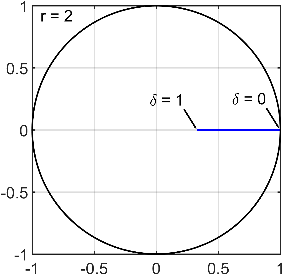
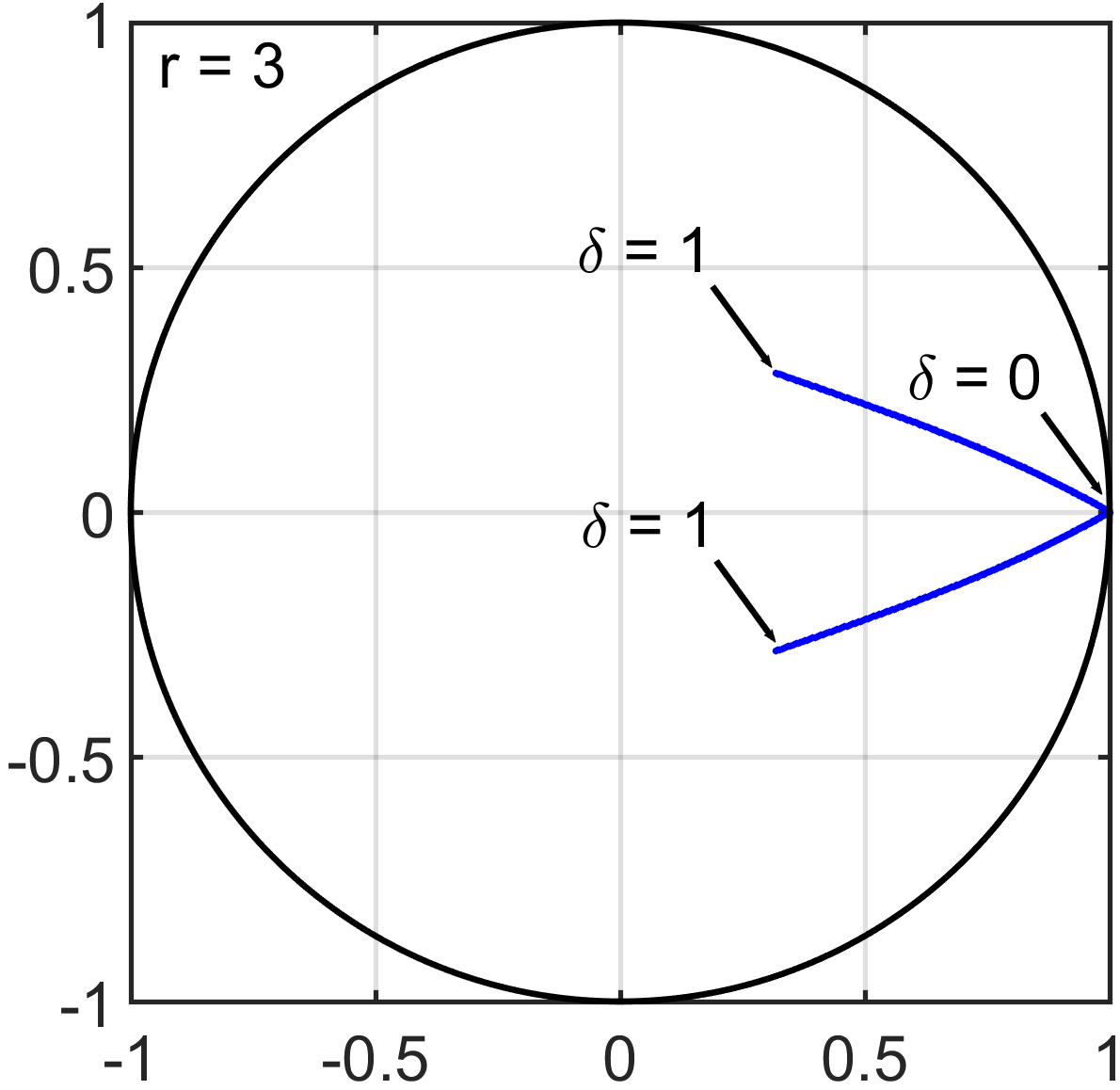
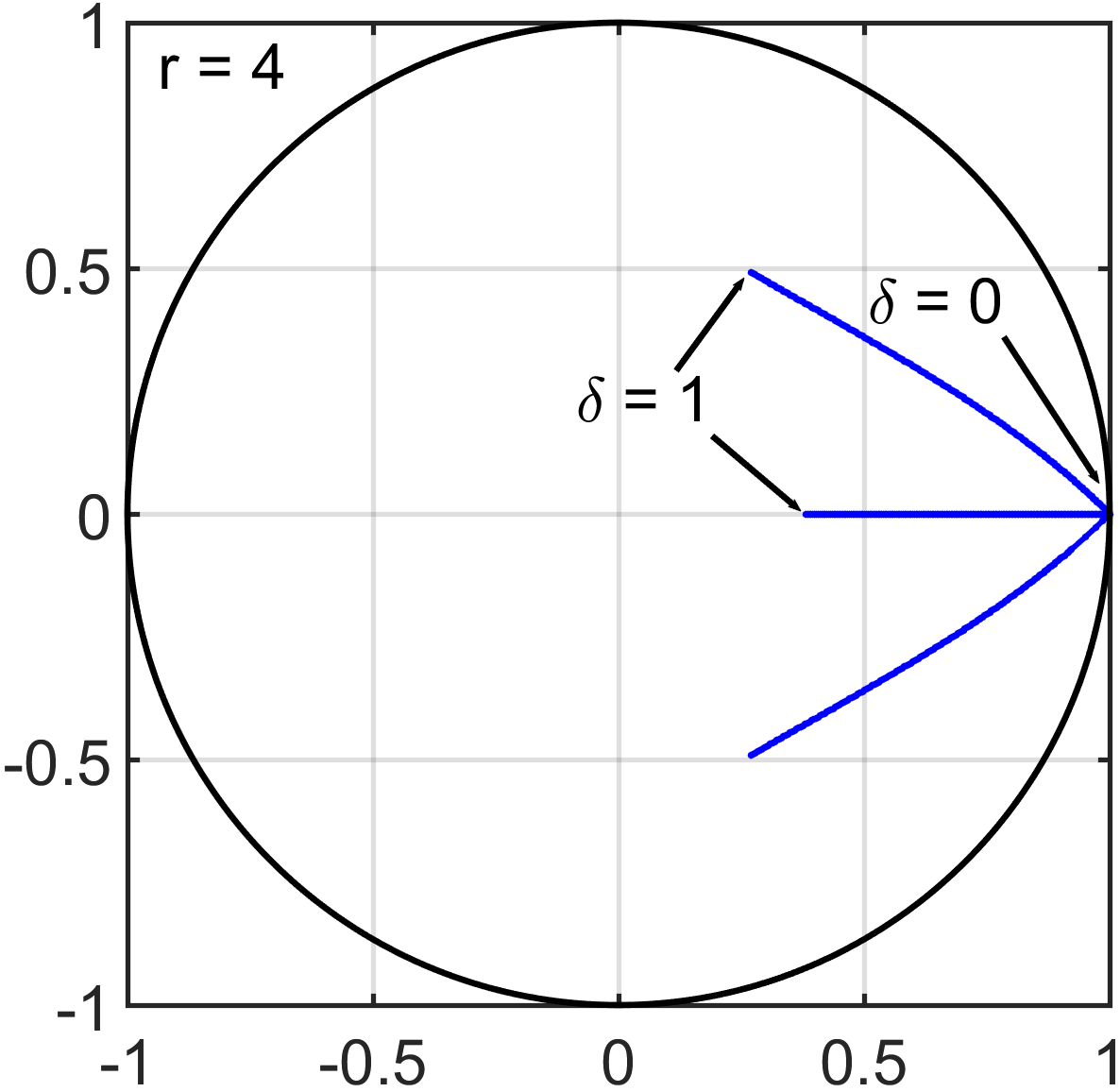
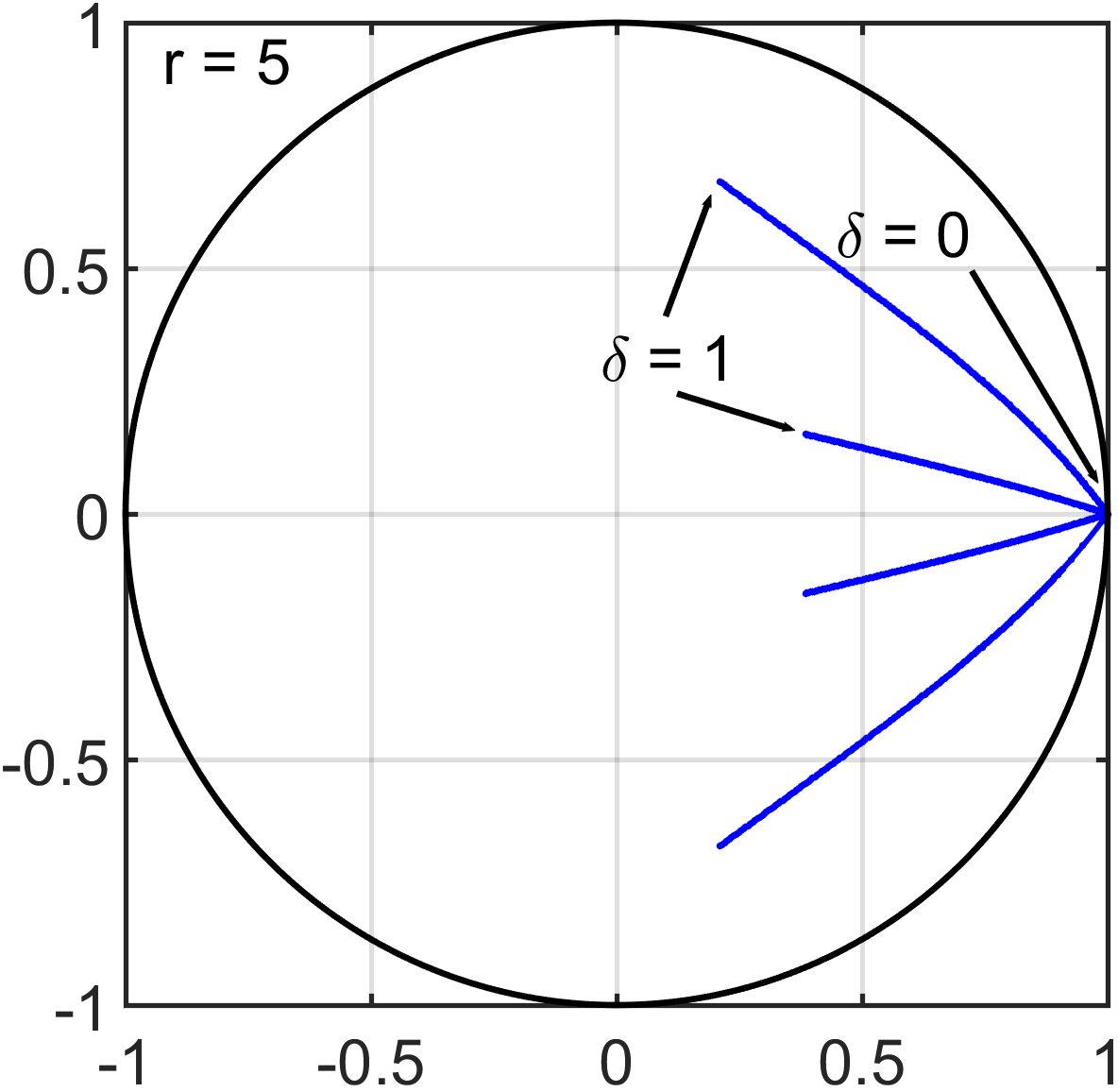
Figure 7: Zero stability for the new ImEx coefficients defined by (4.1)–(4.3), and orders $r=2$–$5\/$. The blue curve shows the roots of $a(z)$ in the complex plane for different $\delta$. Note $z=1$ is a root for all $\delta$ since $a(1)=0$. The remaining $r-1$ roots remain strictly inside the unit circle for all $0<\delta\leq 1$, and approach $z=1$ as $\delta\rightarrow 0$.

Appendix C Numerical test: Global Truncation Error constant

To numerically examine the $\delta$-dependence on the error, we compute the GTE of the test ODE:

$$u_{t}=-u,$$ (C.1)

where $\mbox{\boldmath$A$}u=-u$ (and $\mbox{\boldmath$B$}u=0$). We take a final integration time $t=1$, $u^{*}(1)=e^{-1}$. We perform tests with two different sets of time steps $k$:

• Table 2 shows the GTE (scales as $\delta^{-r}$), and error rates for a fixed $k=10^{-3}$ and variable $\delta$ values.

• Table 3 shows the GTE for different $\delta$ values, with a time step $k=\frac{1}{5}\delta$ taken as a fixed fraction of $\delta$. The table shows that the GTE is approximately constant over decreasing $\delta$, and decreases by $\big{(}\frac{k}{\delta}\big{)}^{r}=\big{(}\frac{1}{5}\big{)}^{r}$ with the order.

$\delta$	$r=1$	Rate	$r=2$	Rate	$r=3$	Rate	$r=4$	Rate	$r=5$	Rate
$2^{0}$	1.839e-04	-	1.227e-07	-	9.203e-11	-	7.370e-14	-	1.030e-17	-
$2^{-1}$	5.514e-04	-1.58	8.587e-07	-2.81	1.381e-09	-3.91	2.284e-12	-4.95	2.304e-15	-7.81
$2^{-2}$	1.285e-03	-1.22	4.539e-06	-2.40	1.611e-08	-3.54	5.754e-11	-4.65	1.663e-13	-6.17
$2^{-3}$	2.749e-03	-1.10	2.073e-05	-2.19	1.560e-07	-3.28	1.175e-09	-4.35	8.027e-12	-5.59
$2^{-4}$	5.658e-03	-1.04	8.838e-05	-2.09	1.371e-06	-3.14	2.126e-08	-4.18	3.138e-10	-5.29
$2^{-5}$	1.141e-02	-1.01	3.637e-04	-2.04	1.144e-05	-3.06	3.589e-07	-4.08	1.095e-08	-5.13
$2^{-6}$	2.263e-02	-0.99	1.454e-03	-2.00	9.160e-05	-3.00	5.681e-06	-3.98	3.438e-07	-4.97
$2^{-3}$	2.7e-03	-1.10	2.1e-05	-2.19	1.6e-07	-3.28	1.2e-09	-4.35	8.0e-12	-5.59
$2^{-4}$	5.7e-03	-1.04	8.8e-05	-2.09	1.4e-06	-3.14	2.1e-08	-4.18	3.1e-10	-5.29
$2^{-5}$	1.1e-02	-1.01	3.6e-04	-2.04	1.1e-05	-3.06	3.6e-07	-4.08	1.1e-08	-5.13
$2^{-6}$	2.3e-02	-0.99	1.5e-03	-2.00	9.2e-05	-3.00	5.7e-06	-3.98	3.4e-07	-4.97

Table 2: Global truncation error. Error rates varying $\delta$ with fixed $k=10^{-3}$ for the equation $u_{t}=-u$. Calculations for orders $r=4,5$ required 64 digits of accuracy. Errors for $\delta=2^{-2}$ are not shown, but used to compute rates for the values $\delta=2^{-3}$.

$\delta$	$r=1$	$r=2$	$r=3$	$r=4$	$r=5$
$2^{0}$	3.400e-02	5.047e-03	8.545e-04	1.509e-04	2.704e-05
$2^{-1}$	5.102e-02	7.967e-03	1.278e-03	2.043e-04	3.239e-05
$2^{-2}$	5.903e-02	9.766e-03	1.573e-03	2.404e-04	3.480e-05
$2^{-3}$	6.291e-02	1.069e-02	1.728e-03	2.587e-04	3.584e-05
$2^{-4}$	6.482e-02	1.116e-02	1.804e-03	2.673e-04	3.618e-05
$2^{-5}$	6.577e-02	1.139e-02	1.842e-03	2.713e-04	3.629e-05
$2^{-6}$	6.625e-02	1.150e-02	1.860e-03	2.732e-04	3.753e-05
$2^{-7}$	6.648e-02	1.156e-02	1.870e-03	2.742e-04	3.592e-05
$2^{-8}$	6.660e-02	1.159e-02	1.874e-03	2.718e-04	3.634e-05
$2^{-9}$	6.666e-02	1.160e-02	1.877e-03	2.818e-04	3.634e-05
$2^{-10}$	6.669e-02	1.161e-02	1.878e-03	2.750e-04	3.635e-05

Table 3: Global truncation error fixing $k=\frac{1}{5}\delta$ for the equation $u_{t}=-u$. Note that the overall error decreased by $\sim\frac{1}{5}$ with each order, and remains constant with a decrease in $\delta$. Numbers in bold required 64 digits of accuracy in the computation.

Appendix D Systematic study of second order ImEx coefficients

The purpose of this section is to show systematically the following necessary condition for large regions of unconditional stability in second order ImEx LMMs: The roots of $c(z)$ must become close to $1$. An ImEx scheme of order $r$ with $s=r$-steps is characterized by $r$ parameters. The proposed coefficients in Definition 4.1 only exploit a one-parameter family of ImEx coefficients. Instead, here we examine ImEx coefficients that arise from a polynomial $c(z)$ with complex roots.

Schemes with $r=s=2$ are characterized by

$$c(z) =(z-\sigma)(z-\bar{\sigma})=z^{2}-(\sigma+\bar{\sigma})z+|\sigma|^{2}.$$

$$b(z) =c(z)-(z-1)^{2}=[2-(\sigma+\bar{\sigma})]z+|\sigma|^{2}-1=Az-B,$$

where $A=2-(\sigma+\bar{\sigma})$, $B=1-|\sigma|^{2}$. Note that the roots of $c(z)$ must satisfy $|\sigma|\leq 1$ for unconditional stability and hence $A,B$ are real and $0\leq A\leq 4$, $0\leq B\leq 1$.

The boundary of the limiting stability region $\mathcal{D}_{-\infty}$ takes the form:

$$\frac{c(z)}{b(z)}=\frac{z^{2}-Az+B-1}{Az-B},\quad\textrm{such that }|z|=1.$$

Note that the numerator $|c(z)|\leq 1+4=5$ is bounded. Therefore for $\mathcal{D}_{-\infty}$ to be large, the denominator $b(z)$ must become small. Examining $b(z)$ we have

$$|b(z)|^{2} =(Az-B)(A\bar{z}-B)=A^{2}+B^{2}-2AB\;\textrm{Re }z,\quad\quad-1\leq\textrm{Re }z\leq 1$$

$$\geq A^{2}+B^{2}-2AB=(A-B)^{2}\geq 0.$$

Therefore the denominator $b(z)$ is bounded away from $0$, unless $A\approx B$. Here

$$(A-B)=(\sigma-1)(\bar{\sigma}-1).$$

Therefore, a necessary condition for a large stability region is to have the roots $\sigma=1-\delta$ for some arbitrary complex $\delta\in\mathbb{C}$ with $|\delta|\ll 1$. The polynomials $b(z),c(z)$ are then

$$b(z)=2(\textrm{Re}\;\delta)\;z-2\textrm{Re}\;\delta-|\delta|^{2},\quad c(z)=(z-1+\delta)(z-1+\bar{\delta}).$$

Computing the implicit GTE error constant in equation (4.20) yields

$$C_{I,r}=|\delta|^{-2}\Big{(}\frac{-74}{6}-\frac{35}{6}|\delta|^{2}+\frac{563}{36}\textrm{Re }\delta\Big{)}=\mathcal{O}(|\delta|^{-2}),\quad|\delta|\rightarrow 0.$$

Therefore, large regions of unconditional stability are accompanied by a decrease in the error constant (when applied to arbitrary general initial data).

One can also examine the case where the polynomial $c(z)$ has real, but unequal, roots.

References

- [1] A. Abdulle and A. A. Medovikov, Second order Chebyshev methods based on orthogonal polynomials, Numer. Math., 90 (2001), pp. 1–18.
- [2] L. Ahlfors, Complex analysis, McGraw-Hill, Inc., third ed., 1979.
- [3] G. Akrivis, Implicit-explicit multistep methods for nonlinear parabolic equations, Mathematics of Computation, 82 (2012), pp. 45–68.
- [4] G. Akrivis, M. Crouzeix, and C. Makridakis, Implicit-explicit multistep finite element methods for nonlinear parabolic problems, Mathematics of Computation, 67 (1998), pp. 457–477.
- [5] , Implicit-explicit multistep methods for quasilinear parabolic equations, Numer. Math, 82 (1999), pp. 521–541.
- [6] G. Akrivis and F. Karakatsani, Modified implicit-explicit BDF methods for nonlinear parabolic equations, BIT Numerical Mathematics, 43 (2003), pp. 467–483.
- [7] M. Anitescu, W. Layton, and F. Pahlevani, Implicit for local effects, explicit for nonlocal is unconditionally stable, ETNA, 18 (2004), pp. 174–187.
- [8] U. Ascher, S. J. Ruuth, and B. Wetton, Implicit-explicit methods for time dependent partial differential equations, SIAM J. Numer. Anal., 32 (1995), pp. 797–823.
- [9] V. Badalassi, H. Ceniceros, and S. Banerjee, Computation of multiphase systems with phase field models, J. Comput. Phys., 190 (2003), pp. 371–397.
- [10] A. Bertozzi, N. Ju, and J.-W. Lu, A biharmonic-modified forward time stepping method for fourth order nonlinear diffusion equations, Discrete and continuous dynamical systems, 29 (2011), pp. 1367–1391.
- [11] J. Cahn and J. Hilliard, Free energy of a nonuniform system I. interfacial free energy, J. Chem. Phys., 28 (1958), pp. 258–267.
- [12] H. Ceniceros, A semi-implicit moving mesh method for the focusing nonlinear Schroedinger equation, Comm. on Pure and Appl. Anal., 1 (2002), pp. 1–14.
- [13] A. Christlieb, J. Jones, K. Promislow, B. Wetton, and M. Willoughby, High accuracy solutions to energy gradient flows from material science models, J. Comput. Phys., 257 (2014), pp. 193–215.
- [14] P. Concus and G. H. Golub, Use of fast direct methods for the efficient numerical solution of nonseparable elliptic equations, SIAM J. Numer. Anal., 10 (1973), pp. 1103–1120.
- [15] M. Crouzeix, Une méthode multipas implicite-explicite pour l’approximation des équations d’évolution paraboliques, Numer. Math, 35 (1980), pp. 257–276.
- [16] J. Douglas and T. Dupont, Alternating-direction Galerkin methods on rectangles, in Numerical Solution of Partial Differential Equations, B. Hubbard, ed., vol. II, College Park, Md., 1971, SYNSPADE-1970, Univ. of Maryland, Academic Press, New York, pp. 133–213.
- [17] T. A. Driscoll, N. Hale, and L. N. Trefethen, Chebfun guide, 2014. Code title: Field of values and numerical abscissa.
- [18] M. Elsey and B. Wirth, A simple and efficient scheme for phase field crystal simulation, M2AN, 47 (2013), pp. 1413–1432.
- [19] D. Eyre, Unconditionally gradient stable time marching the Cahn-Hilliard equation, in Computational and Mathematical Models of Microstructural Evolution, J. W. Bullard, R. Kalia, M. Stoneham, and L. Chen, eds., vol. 53, Warrendale, PA, USA, 1998, Materials Research Society, pp. 1686–1712.
- [20] J. Frank, W. Hundsdorfer, and J. Verwer, On the stability of IMEX LM methods, Appl. Numer. Math., 25 (1997), pp. 193––205.
- [21] K. Glasner, A diffuse interface approach to Hele-Shaw flow, Nonlinearity, 16 (2003), pp. 49–66.
- [22] K. Glasner and S. Orizaga, Improving the accuracy of convexity splitting methods for gradient flow equations, J. Comput. Phys., 315 (2016), pp. 52–64.
- [23] D. Gottlieb and B. Orszag, Numerical Analysis of Spectral Methods, CBMS-NSF Regional Conference Series in Applied Mathematics, SIAM Press, 1977.
- [24] L. Greengard and V. Rokhlin, A fast algorithm for particle simulations, J. Comput. Phys., 73 (1987), pp. 325–348.
- [25] Z. Guan, J. Lowengrub, C. Wang, and S. Wise, Second-order convex splitting schemes for periodic nonlocal Cahn-Hilliard and Allen-Cahn equations, J. Comput. Phys., 277 (2014), pp. 48–71.
- [26] E. Hairer, S. P. Nørsett, and G. Wanner, Solving ordinary differential equations I: Nonstiff problems, Springer-Verlag, Berlin, second revised edition ed., 1987.
- [27] E. Hairer and G. Wanner, Solving ordinary differential equations II: Stiff and Differential-Algebraic Problems, vol. 1, Springer-Verlag, Berlin, 1991.
- [28] A. Horn and C. Johnson, Topics in Matrix analysis, Cambridge University Press, 1991.
- [29] W. Hundsdorfer and J. Verwer, Numerical Solution of Time-Dependent Advection-Diffusion-Reaction Equations, Springer Series in Comput. Math. 33, Springer, 2003.
- [30] R. Jeltsch and O. Nevanlinna, Stabiliity of explicit time discretizations for solving initial value problems, Numer. Math., 37 (1981), pp. 61–91.
- [31] , Stability and accuracy of time discretizations for initial value problems, Numer. Math., 40 (1982), pp. 245–296.
- [32] C. R. Johnson, Numerical determination of the field of values of a general complex matrix, SIAM J. Numer. Anal., 15 (1978), pp. 595–602.
- [33] H. Johnston and J.-G. Liu, Accurate, stable and efficient Navier-Stokes solvers based on explicit treatment of the pressure term, J. Comput. Phys., 199 (2004), pp. 221–259.
- [34] L. Ju, J. Zhang, L. Zhu, and Q. Du, Fast explicit integration factor methods for semilinear parabolic equations, J. Sci. Comput., 62 (2015), pp. 431–455.
- [35] G. Karniadakis, M. Israeli, and S. A. Orszag, High-order splitting methods for the incompressible Navier-Stokes equations, J. Comput. Phys., 97 (1991), pp. 414–443.
- [36] J. Kim and P. Moin, Application of a fractional step method to incompressible Navier-Stokes equations, J. Comput. Phys., 59 (1985), pp. 308–323.
- [37] T. Koto, Stability of implicit-explicit linear multistep methods for ordinary and delay differential equations, Front. Math. China, 4 (2009), pp. 113–129.
- [38] W. Layton and C. Trenchea, Stability of two IMEX methods, CNLF and BDF2-AB2, for uncoupling systems of evolution equations, Appl. Numer. Math., 62 (2012), pp. 112––120.
- [39] R. J. LeVeque, Finite difference methods for ordinary and partial differential equations: Steady-state and time-dependent problems, Society for Industrial and Applied Mathematics, first ed., 2007.
- [40] J.-G. Liu, J. Liu, and R. L. Pego, Stability and convergence of efficient Navier-Stokes solvers via a commutator estimate, Comm. Pure Appl. Math., 60 (2007), pp. 1443–1487.
- [41] , Stable and accurate pressure approximation for unsteady incompressible viscous flow, J. Comput. Phys., 229 (2010), pp. 3428–3453.
- [42] P. A. Milewski and E. G. Tabak, A pseudo-spectral algorithm for the solution of nonlinear wave equations, SIAM J. Sci. Comput., 21 (1999), pp. 1102–1114.
- [43] M. L. Minion, Semi-implicit spectral deferred correction methods for ordinary differential equations, Commun. Math Sci., 1 (2003), pp. 471–500.
- [44] G. Sheng, T. Wang, Q. Du, K. Wang, Z. Liu, and L. Q. Chen, Coarsening kinetics of a two phase mixture with highly disparate diffusion mobility, Commun. Comput. Phys., 8 (2010), pp. 249–264.
- [45] D. Shirokoff and R. R. Rosales, An efficient method for the incompressible Navier-Stokes equations on irregular domains with no-slip boundary conditions, high order up to the boundary, J. Comput. Phys., 230 (2011), pp. 8619–8646.
- [46] P. Smereka, Semi-implicit level set methods for curvature and surface diffusion motion, J. Sci. Comput., 19 (2003), pp. 439–456.
- [47] L. N. Trefethen, Spectral Methods in MATLAB, SIAM, Philadelphia, 2000.
- [48] L. N. Trefethen and D. Bau, Numerical Linear Algebra, SIAM, Philadelphia, 2000.
- [49] C. Trenchea, Second order implicit for local effects and explicit for nonlocal effects is unconditionally stable, Romai J., 12 (2016), pp. 163–178.
- [50] J. M. Varah, Stability restrictions on second order, three level finite difference schemes for parabolic equations, SIAM J. Numer. Anal., 17 (1980), pp. 300–309.
- [51] J. Xu, Y. Li, and S. Wu, Convex splitting schemes interpreted as fully implicit schemes in disguise for phase field modeling, 2016. arXiv:1604.05402.
- [52] Y. Yan, W. Chen, C. Wang, and S. Wise, A second-order energy stable BDF numerical scheme for the Cahn-Hilliard equation, 2015.