Private Topic Modeling

Abstract

We develop a privatised stochastic variational inference method for Latent Dirichlet Allocation (LDA). The iterative nature of stochastic variational inference presents challenges: multiple iterations are required to obtain accurate posterior distributions, yet each iteration increases the amount of noise that must be added to achieve a reasonable degree of privacy. We propose a practical algorithm that overcomes this challenge by combining: (1) an improved composition method for differential privacy, called the moments accountant, which provides a tight bound on the privacy cost of multiple variational inference iterations and thus significantly decreases the amount of additive noise; and (2) privacy amplification resulting from subsampling of large-scale data. Focusing on conjugate exponential family models, in our private variational inference, all the posterior distributions will be privatised by simply perturbing expected sufficient statistics. Using Wikipedia data, we illustrate the effectiveness of our algorithm for large-scale data.

1 Background

Differential Privacy

(DP) is a formal definition of the privacy properties of data analysis algorithms [1, 2]. A randomized algorithm $\mathcal{M}(\mathbf{X})$ is said to be $(\epsilon,\delta)$-differentially private if

$$Pr(\mathcal{M}(\mathbf{X})\in\mathcal{S})\leq\exp(\epsilon)Pr(\mathcal{M}(\mathbf{X}^{\prime})\in\mathcal{S})+\delta$$ (1)

for all measurable subsets $\mathcal{S}$ of the range of $\mathcal{M}$ and for all datasets $\mathbf{X}$, $\mathbf{X}^{\prime}$ differing by a single entry (either by excluding that entry or replacing it with a new entry). Here, an entry usually corresponds to a single individual’s private value. If $\delta=0$, the algorithm is said to be $\epsilon$-differentially private, and if $\delta>0$, it is said to be approximately differentially private. Intuitively, the definition states that the probability of any event does not change very much when a single individual’s data is modified, thereby limiting the amount of information that the algorithm reveals about any one individual. We observe that $\mathcal{M}$ is a randomized algorithm, and randomization is achieved by either adding external noise, or by subsampling. In this paper, we use the “include/exclude” version of DP, in which differing by a single entry refers to the inclusion or exclusion of that entry in the dataset.

Variational inference for the conjugate exponential models

Variational inference is an optimization-based posterior inference method, which simplifies to a two-step procedure when the model falls into the Conjugate-Exponential (CE) class of models. CE family models satisfy two conditions [3]:

$$(1)\mbox{ The complete-data likelihood is in the exponential family}:$$

$$\qquad p(\mathcal{D}_{n},\mathbf{\bm{\mathit{l}}}_{n}|\mathbf{\bm{\mathit{m}}})=g(\mathbf{\bm{\mathit{m}}})f(\mathcal{D}_{n},\mathbf{\bm{\mathit{l}}}_{n})\exp(\mathbf{n}(\mathbf{\bm{\mathit{m}}}){{}^{\top}}\mathbf{s}(\mathcal{D}_{n},\mathbf{\bm{\mathit{l}}}_{n})),$$ (2)

$$(2)\mbox{ The prior over $\mathbf{\bm{\mathit{m}}}$ is conjugate to the complete-data likelihood}:$$

$$\qquad p(\mathbf{\bm{\mathit{m}}}|\tau,\mathbf{\bm{\nu}})=h(\tau,\mathbf{\bm{\nu}})g(\mathbf{\bm{\mathit{m}}})^{\tau}\exp(\mathbf{\bm{\nu}}{{}^{\top}}\mathbf{n}(\mathbf{\bm{\mathit{m}}})).$$ (3)

where natural parameters and sufficient statistics of the complete-data likelihood are denoted by $\mathbf{n}(\mathbf{\bm{\mathit{m}}})$ and $\mathbf{s}(\mathcal{D}_{n},\mathbf{\bm{\mathit{l}}}_{n})$, respectively, and $g,f,h$ are some known functions. The hyperparameters are denoted by $\tau$ (a scalar) and $\mathbf{\bm{\nu}}$ (a vector).

The variational inference algorithm for a CE family model optimises the lower bound on the model log marginal likelihood given by,

$$\mathcal{L}(q(\mathbf{\bm{\mathit{l}}})q(\mathbf{\bm{\mathit{m}}}))=\int d\mathbf{\bm{\mathit{m}}}\;d\mathbf{\bm{\mathit{l}}}\;q(\mathbf{\bm{\mathit{l}}})q(\mathbf{\bm{\mathit{m}}})\log\frac{p(\mathbf{\bm{\mathit{l}}},\mathcal{D},\mathbf{\bm{\mathit{m}}})}{q(\mathbf{\bm{\mathit{l}}})q(\mathbf{\bm{\mathit{m}}})},$$ (4)

where we assume that the joint approximate posterior distribution over the latent variables and model parameters $q(\mathbf{\bm{\mathit{l}}},\mathbf{\bm{\mathit{m}}})$ is factorised via the mean-field assumption as $q(\mathbf{\bm{\mathit{l}}},\mathbf{\bm{\mathit{m}}})=q(\mathbf{\bm{\mathit{l}}})q(\mathbf{\bm{\mathit{m}}})=q(\mathbf{\bm{\mathit{m}}})\prod_{n=1}^{N}q(\mathbf{\bm{\mathit{l}}}_{n}),$ and that each of the variational distributions also has the form of an exponential family distribution. Computing the derivatives of the variational lower bound in Eq. 4 with respect to each of these variational distributions and setting them to zero yield the following two-step procedure.

$$(1)\mbox{ First, given expected natural parameters $\bar{\mathbf{n}}$, the E-step computes:}$$

$$\qquad q(\mathbf{\bm{\mathit{l}}})=\prod_{n=1}^{N}q(\mathbf{\bm{\mathit{l}}}_{n})\propto\prod_{n=1}^{N}f(\mathcal{D}_{n},\mathbf{\bm{\mathit{l}}}_{n})\exp(\bar{\mathbf{n}}{{}^{\top}}\mathbf{s}(\mathcal{D}_{n},\mathbf{\bm{\mathit{l}}}_{n}))=\prod_{n=1}^{N}p(\mathbf{\bm{\mathit{l}}}_{n}|\mathcal{D}_{n},\bar{\mathbf{n}}).$$ (5)

Using $$q(\mathbf{\bm{\mathit{l}}}) {\mathbf{s}}(\mathcal{D}_{n},\mathbf{\bm{\mathit{l}}}_{n})$$, it outputs expected sufficient statistics, the expectation of

$$\qquad\mbox{with probability density $q(\mathbf{\bm{\mathit{l}}}_{n})$ : }\bar{\mathbf{s}}(\mathcal{D})=\tfrac{1}{N}\sum_{n=1}^{N}\langle{\mathbf{s}}(\mathcal{D}_{n},\mathbf{\bm{\mathit{l}}}_{n})\rangle_{q(\mathbf{\bm{\mathit{l}}}_{n})}.$$

$$(2)\mbox{ Second, given expected sufficient statistics $\bar{\mathbf{s}}(\mathcal{D})$, the M-step computes:}$$

$$\qquad q(\mathbf{\bm{\mathit{m}}})=h(\tilde{\tau},\tilde{\mathbf{\bm{\nu}}})g(\mathbf{\bm{\mathit{m}}})^{\tilde{\tau}}\exp(\tilde{\mathbf{\bm{\nu}}}{{}^{\top}}\mathbf{n}(\mathbf{\bm{\mathit{m}}})),\mbox{ where }\tilde{\tau}=\tau+N,\;\tilde{\mathbf{\bm{\nu}}}=\mathbf{\bm{\nu}}+N\bar{\mathbf{s}}(\mathcal{D}).$$ (6)

$$\qquad\mbox{Using $q(\mathbf{\bm{\mathit{m}}})$, it outputs expected natural parameters $\bar{\mathbf{n}}=\langle\mathbf{n}(\mathbf{\bm{\mathit{m}}})\rangle_{q(\mathbf{\bm{\mathit{m}}})}$}.$$

2 Privacy preserving VI algorithm for CE family

The only place where the algorithm looks at the data is when computing the expected sufficient statistics $\bar{\mathbf{s}}(\mathcal{D})$ in the first step. The expected sufficient statistics then dictates the expected natural parameters in the second step. So, perturbing the sufficient statistics leads to perturbing both posterior distributions $q(\mathbf{\bm{\mathit{l}}})$ and $q(\mathbf{\bm{\mathit{m}}})$. Perturbing sufficient statistics in exponential families is also used in [4]. Existing work focuses on privatising posterior distributions in the context of posterior sampling [5, 6, 7, 8], while our work focuses on privatising approximate posterior distributions for optimisation-based approximate Bayesian inference. Suppose there are two neighbouring datasets $\mathcal{D}$ and $\mathcal{D}^{\prime}$, where there is only one datapoint difference among them. We also assume that the dataset is pre-processed such that the L2 norm of any datapoint is less than 1. The maximum difference in the expected sufficient statistics given the datasets, e.g., the L-1 sensitivity of the expected sufficient statistics is given by (assuming s is a vector of length L) $\Delta\mathbf{s}=\max_{\mathcal{D},\mathcal{D}^{\prime},q(\mathbf{\bm{\mathit{l}}}),q(\mathbf{\bm{\mathit{l}}}^{\prime})}\sum_{l=1}^{L}\frac{1}{N}|\mathbb{E}_{q(\mathbf{\bm{\mathit{l}}})}\mathbf{s}_{l}(\mathcal{D},\mathbf{\bm{\mathit{l}}})-\mathbb{E}_{q(\mathbf{\bm{\mathit{l}}}^{\prime})}\mathbf{s}_{l}(\mathcal{D}^{\prime},\mathbf{\bm{\mathit{l}}}^{\prime})|$.Under some models like LDA below, expected sufficient statistic has a limited sensitivity, in which case we add noise to each coordinate of the expected sufficient statistics to compensate the maximum change.

3 Privacy preserving latent Dirichlet allocation (LDA)

The most successful topic modeling is based on LDA, where the generative process is given by [9]. Its generative process is given by

• Draw topics $\mathbf{\bm{\beta}}_{k}\sim$ Dirichlet $(\eta\mathbf{1}_{V})$, for $k=\{1,\ldots,K\}$, where $\eta$ is a scalar hyperarameter.

• For each document $d\in\{1,\ldots,D\}$

  • Draw topic proportions $\mathbf{\bm{\theta}}_{d}\sim$ Dirichlet $(\alpha\mathbf{1}_{K})$, where $\alpha$ is a scalar hyperarameter.

  • For each word $n\in\{1,\ldots,N\}$

    • Draw topic assignments $\mathbf{z}_{dn}\sim$ Discrete$(\mathbf{\bm{\theta}}_{d})$

    • Draw word $\mathbf{w}_{dn}\sim$ Discrete$(\mathbf{\bm{\beta}}_{\mathbf{z}_{dn}})$

where each observed word is represented by an indicator vector $\mathbf{w}_{dn}$ ($n$th word in the $d$th document) of length $V$, and where $V$ is the number of terms in a fixed vocabulary set. The topic assignment latent variable $\mathbf{z}_{dn}$ is also an indicator vector of length $K$, where $K$ is the number of topics. The LDA model falls in the CE family, viewing $\mathbf{z}_{d,1:N}$ and $\mathbf{\bm{\theta}}_{d}$ as two types of latent variables: $\mathbf{\bm{\mathit{l}}}_{d}=\{\mathbf{z}_{d,1:N},\mathbf{\bm{\theta}}_{d}\}$, and $\mathbf{\bm{\beta}}$ as model parameters $\mathbf{\bm{\mathit{m}}}=\mathbf{\bm{\beta}}$. The conditions for CE are satisfied: (1) the complete-data likelihood is in exponential family: $p(\mathbf{w}_{d,1:N},\mathbf{z}_{d,1:N},\mathbf{\bm{\theta}}_{d}|\mathbf{\bm{\beta}})\propto f(\mathcal{D}_{d},\mathbf{z}_{d,1:N},\mathbf{\bm{\theta}}_{d})\exp(\sum_{n}\sum_{k}[\log\mathbf{\bm{\beta}}_{k}]{{}^{\top}}[\mathbf{z}_{dn}^{k}\mathbf{w}_{dn}]),$ where $f(\mathcal{D}_{d},\mathbf{z}_{d,1:N},\mathbf{\bm{\theta}}_{d})\propto\exp([\alpha\mathbf{1}_{K}]{{}^{\top}}[\log\mathbf{\bm{\theta}}_{d}]+\sum_{n}\sum_{k}\mathbf{z}_{dn}^{k}\log\mathbf{\bm{\theta}}_{d}^{k})$; and (2) we have a conjugate prior over $\mathbf{\bm{\beta}}_{k}$: $p(\mathbf{\bm{\beta}}_{k}|\eta\mathbf{1}_{V})\propto\exp([\eta\mathbf{1}_{V}]{{}^{\top}}[\log\mathbf{\bm{\beta}}_{k}]),$ for $k=\{1,\ldots,K\}$. For simplicity, we assume hyperparameters $\alpha$ and $\eta$ are set manually. Under the LDA model, we assume the variational posteriors are given by

• Discrete : $q(\mathbf{z}_{dn}^{k}|\mathbf{\bm{\phi}}_{dn}^{k})\propto\exp(\mathbf{z}_{dn}^{k}\log\mathbf{\bm{\phi}}_{dn}^{k})$, with variational parameters for capturing the posterior topic assignment, $\mathbf{\bm{\phi}}_{dn}^{k}\propto\exp(\langle\log\mathbf{\bm{\beta}}_{k}\rangle_{q(\mathbf{\bm{\beta}}_{k})}{{}^{\top}}\mathbf{w}_{dn}+\langle\log\mathbf{\bm{\theta}}_{d}^{k}\rangle_{q(\mathbf{\bm{\theta}}_{d})}).$

• Dirichlet : $q(\mathbf{\bm{\theta}}_{d}|\mathbf{\bm{\gamma}}_{d})\propto\exp(\mathbf{\bm{\gamma}}_{d}{{}^{\top}}\log\mathbf{\bm{\theta}}_{d}),\mbox{where }\mathbf{\bm{\gamma}}_{d}=\alpha\mathbf{1}_{K}+\sum_{n=1}^{N}\langle\mathbf{z}_{dn}\rangle_{q(\mathbf{z}_{dn})}$,

where these two distributions are computed in the E-step behind the privacy wall. The expected sufficient statistics are $\bar{\mathbf{s}}_{k}^{v}=\tfrac{1}{D}\sum_{d}\sum_{n}\langle\mathbf{z}_{dn}^{k}\rangle_{q(\mathbf{z}_{dn})}\mathbf{w}^{v}_{dn}=\tfrac{1}{D}\sum_{d}\sum_{n}\mathbf{\bm{\phi}}_{dn}^{k}\mathbf{w}_{dn}$. Then, in the M-step, we compute the posterior

• Dirichlet : $q(\mathbf{\bm{\beta}}_{k}|\mathbf{\bm{\lambda}}_{k})\propto\exp(\mathbf{\bm{\lambda}}_{k}{{}^{\top}}\log\mathbf{\bm{\beta}}_{k}),\mbox{ where }\mathbf{\bm{\lambda}}_{k}=\eta\mathbf{1}_{V}+\sum_{d}\sum_{n}\langle\mathbf{z}_{dn}^{k}\rangle_{q(\mathbf{z}_{dn})}\mathbf{w}_{dn}$.

Sensitivity analysis

In a large-scale data setting, it is impossible to handle the entire dataset at once. In such case, stochastic learning using noisy sufficient statistics computed on mini-batches of data. At each learning step with a freshly drawn mini-batch of data (size $S$), we perturb the expected sufficient statistics. While each document has a different document length $N_{d}$, we limit the maximum length of any document to $N$ by randomly selecting $N$ words in a document if the number of words in the document is longer than $N$.

We add Gaussian noise to each component of the expected sufficient statistics, which is a matrix of size $K\times V$,

$$\tilde{\bar{\mathbf{s}}}_{k}^{v}={\bar{\mathbf{s}}}_{k}^{v}+Y_{k}^{v},\mbox{ where }Y_{k}^{v}\sim\mathcal{N}(0,\sigma^{2}(\Delta\bar{\mathbf{s}})^{2}),$$ (7)

where $\bar{\mathbf{s}}_{k}^{v}=\tfrac{1}{S}\sum_{d}\sum_{n}\mathbf{\bm{\phi}}_{dn}^{k}\mathbf{w}_{dn}^{v}$, and $\Delta\bar{\mathbf{s}}$ is the sensitivity. We then map the perturbed components to 0 if they become negative. For LDA, the worst-case sensitivity is given by

$$\Delta\bar{\mathbf{s}} =\max_{|\mathcal{D}\setminus{\mathcal{D}^{\prime}}|=1}\sqrt{\sum_{k}\sum_{v}(\bar{\mathbf{s}}_{k}^{v}(\mathcal{D})-\bar{\mathbf{s}}_{k}^{v}(\mathcal{D}^{\prime}))^{2}},$$

$$=\max_{|\mathcal{D}\setminus{\mathcal{D}^{\prime}}|=1}\sqrt{\sum_{k}\sum_{v}\left(\frac{1}{S}\sum_{n}\sum_{d=1}^{S}\mathbf{\bm{\phi}}_{dn}^{k}\mathbf{w}_{dn}^{v}-\frac{1}{S-1}\sum_{n}\sum_{d=1}^{S-1}\mathbf{\bm{\phi}}_{dn}^{k}\mathbf{w}_{dn}^{v}\right)^{2}},$$

$$=\max_{|\mathcal{D}\setminus{\mathcal{D}^{\prime}}|=1}\sqrt{\sum_{k}\sum_{v}\left|\frac{S-1}{S}\frac{1}{S-1}\sum_{n}\sum_{d=1}^{S-1}\mathbf{\bm{\phi}}_{dn}^{k}\mathbf{w}_{dn}^{v}+\frac{1}{S}\sum_{n}\mathbf{\bm{\phi}}_{Sn}^{k}\mathbf{w}_{Sn}^{v}-\frac{1}{S-1}\sum_{n}\sum_{d=1}^{S-1}\mathbf{\bm{\phi}}_{dn}^{k}\mathbf{w}_{dn}^{v}\right|^{2}},$$

$$=\max_{\mathbf{\bm{\phi}}_{Sn}^{k},\mathbf{w}_{Sn}^{v}}\sqrt{\sum_{k}\sum_{v}\left|\frac{1}{S}\sum_{n}\mathbf{\bm{\phi}}_{Sn}^{k}\mathbf{w}_{Sn}^{v}-\frac{1}{S}\left(\frac{1}{S-1}\sum_{n}\sum_{d=1}^{S-1}\mathbf{\bm{\phi}}_{dn}^{k}\mathbf{w}_{dn}^{v}\right)\right|^{2}},$$

$$=\max_{\mathbf{\bm{\phi}}_{Sn}^{k},\mathbf{w}_{Sn}^{v}}\sqrt{\sum_{k}\sum_{v}\left|\frac{1}{S}\sum_{n}\mathbf{\bm{\phi}}_{Sn}^{k}\mathbf{w}_{Sn}^{v}\right|^{2}},$$

since $$0\leq\mathbf{\bm{\phi}}_{dn}^{k}\leq 1 \mathbf{w}_{dn}^{v}\in\{0,1\} 0\leq\frac{1}{S-1}\sum_{n}\sum_{d=1}^{S-1}\mathbf{\bm{\phi}}_{dn}^{k}\mathbf{w}_{dn}^{v}\leq\sum_{n}\mathbf{\bm{\phi}}_{Sn}^{k}\mathbf{w}_{Sn}^{v}$$, , and we assume ,

$$\leq\max_{\mathbf{\bm{\phi}}_{Sn}^{k},\mathbf{w}_{Sn}^{v}}\;\;\frac{1}{S}\sum_{n}(\sum_{k}\mathbf{\bm{\phi}}_{Sn}^{k})(\sum_{v}\mathbf{w}_{Sn}^{v})\leq\frac{N}{S},$$ (8)

since $\sum_{k}\mathbf{\bm{\phi}}_{Sn}^{k}=1$, and $\sum_{v}\mathbf{w}_{Sn}^{v}=1$. This sensitivity accounts for the worst case in which all $NS$ words in the minibatch are assigned to the same entry of $\bar{\mathbf{s}}$, i.e. they all have the same word type $v$, and are hard-assigned to the same topic $k$ in the variational distribution. In our practical implementation, we improve the sensitivity by exploiting the fact that most typical sufficient statistic matrix $\bar{\mathbf{s}}$ given a minibatch (where the size of the matrix is the number of topics by the number of words in the vocabulary set) has a much smaller norm than this worst case. Specifically, inspired by [10], we apply a norm clipping strategy, in which the matrix $\bar{\mathbf{s}}$ is clipped (or projected) such that the Frobenious norm of the matrix is bounded by $|\bar{\mathbf{s}}|\leq a\frac{N}{S}$, for a user-specified $a\in(0,1]$. For each minibatch, if this criterion is not satisfied, we project the expected sufficient statistics down to the required norm via

$$\bar{\mathbf{s}}:=a\frac{N}{S}\frac{\bar{\mathbf{s}}}{{|\bar{\mathbf{s}}|}}\mbox{ .}$$ (9)

After this the procedure, the sensitivity of the entire matrix becomes $a\Delta\bar{\mathbf{s}}$ (i.e., $aN/S$), and we add noise on this scale to the clipped expected sufficient statistics. We set $a=0.1$ in our experiments, which empirically resulted in clipping being applied to around $3/4$ of the documents. The resulting algorithm is summarised in Algorithm 1.

Algorithm 1 Private LDA

0:  Data $\mathcal{D}$. Define $D$ (documents), $V$ (vocabulary), $K$ (number of topics).    Define $\rho_{t}=(\tau_{0}+t)^{-\kappa}$, mini-batch size $S$, hyperparameters $\alpha,\eta$, $\sigma^{2}$, and $a$

0:  Privatised expected natural parameters $\langle\log\mathbf{\bm{\beta}}_{k}\rangle_{q(\mathbf{\bm{\beta}}_{k})}$ and sufficient statistics $\tilde{\bar{\mathbf{s}}}$.

  Compute the sensitivity of the expected sufficient statistics given in Eq. 3.

  for $t=1,\ldots,J$ do

     (1) E-step: Given expected natural parameters $\langle\log\mathbf{\bm{\beta}}_{k}\rangle_{q(\mathbf{\bm{\beta}}_{k})}$

     for $d=1,\ldots,S$ do

        Compute $q(\mathbf{z}_{dn}^{k})$ parameterised by $\mathbf{\bm{\phi}}_{dn}^{k}\propto\exp(\langle\log\mathbf{\bm{\beta}}_{k}\rangle_{q(\mathbf{\bm{\beta}}_{k})}{{}^{\top}}\mathbf{w}_{dn}+\langle\log\mathbf{\bm{\theta}}_{d}^{k}\rangle_{q(\mathbf{\bm{\theta}}_{d})})$.

        Compute $q(\mathbf{\bm{\theta}}_{d})$ parameterised by $\mathbf{\bm{\gamma}}_{d}=\alpha\mathbf{1}_{K}+\sum_{n=1}^{N}\langle\mathbf{z}_{dn}\rangle_{q(\mathbf{z}_{dn})}$.

     end for

     Compute the expected sufficient statistics $\bar{\mathbf{s}}_{k}^{v}=\tfrac{1}{S}\sum_{d}\sum_{n}\mathbf{\bm{\phi}}_{dn}^{k}\mathbf{w}_{dn}^{v}$.

     if $|\bar{\mathbf{s}}|>aN/S$ then

        $\bar{\mathbf{s}}:=a\frac{N}{S}\frac{\bar{\mathbf{s}}}{{|\bar{\mathbf{s}}|}}$

     end if

     Output the perturbed expected sufficient statistics $\tilde{\bar{\mathbf{s}}}_{k}^{v}=\bar{\mathbf{s}}+Y_{k}^{v}$, where $Y_{k}^{v}$ is Gaussian noise given in Eq. 7, but using sensitivity $aN/S$.

     Clip negative entries of $\tilde{\bar{\mathbf{s}}}$ to 0.

     Update the log-moment functions.

     (2) M-step: Given perturbed expected sufficient statistics $\tilde{\bar{\mathbf{s}}}_{k}$,

     Compute $q(\mathbf{\bm{\beta}}_{k})$ parameterised by $\mathbf{\bm{\lambda}}_{k}^{(t)}=\eta\mathbf{1}_{V}+D\tilde{\bar{\mathbf{s}}}_{k}$.

     Set $\mathbf{\bm{\lambda}}^{(t)}\mapsfrom(1-\rho_{t})\mathbf{\bm{\lambda}}^{(t-1)}+\rho_{t}\mathbf{\bm{\lambda}}^{(t)}$.

     Output expected natural parameters $\langle\log\mathbf{\bm{\beta}}_{k}\rangle_{q(\mathbf{\bm{\beta}}_{k})}$.

  end for

4 Privacy analysis of private LDA

We use the Moments Accountant (MA) composition method [10] for accounting for privacy loss incurred by successive iterations of an iterative mechanism. We choose this method as it provides tight privacy bounds (cf., [11]). The moments accountant method is based on the concept of a privacy loss random variable, which allows us to consider the entire spectrum of likelihood ratios $\frac{Pr(\mathcal{M}(\mathbf{X})=o)}{Pr(\mathcal{M}(\mathbf{X}^{\prime})=o)}$ induced by a privacy mechanism $\mathcal{M}$. Specifically, the privacy loss random variable corresponding to a mechanism $\mathcal{M}$, datasets $\mathbf{X}$ and $\mathbf{X^{\prime}}$, and an auxiliary parameter $w$ is a random variable defined as follows: $L_{\mathcal{M}}(\mathbf{X},\mathbf{X^{\prime}},w):=\log\frac{Pr(\mathcal{M}(\mathbf{X},w)=o)}{Pr(\mathcal{M}(\mathbf{X}^{\prime},w)=o)},\quad{\text{with likelihood\ }}Pr(\mathcal{M}(\mathbf{X},w)=o),$ where $o$ lies in the range of $\mathcal{M}$. Observe that if $\mathcal{M}$ is $(\epsilon,0)$-differentially private, then the absolute value of $L_{\mathcal{M}}(\mathbf{X},\mathbf{X^{\prime}},w)$ is at most $\epsilon$ with probability $1$.

The moments accountant method exploits properties of this privacy loss random variable to account for the privacy loss incurred by applying mechanisms $\mathcal{M}_{1},\ldots,\mathcal{M}_{t}$ successively to a dataset $\mathbf{X}$; this is done by bounding properties of the log of the moment generating function of the privacy loss random variable. Specifically, the log moment function $\alpha_{\mathcal{M}_{t}}$ of a mechanism $\mathcal{M}_{t}$ is defined as:

$$\alpha_{\mathcal{M}_{t}}(\lambda)=\sup_{\mathbf{X},\mathbf{X^{\prime}},w}\log\mathbb{E}[\exp(\lambda L_{\mathcal{M}_{t}}(\mathbf{X},\mathbf{X^{\prime}},w))],$$ (10)

where $\mathbf{X}$ and $\mathbf{X^{\prime}}$ are datasets that differ in the private value of a single person. [10] shows that if $\mathcal{M}$ is the combination of mechanisms $(\mathcal{M}_{1},\ldots,\mathcal{M}_{k})$ where each mechanism addes independent noise, then, its log moment generating function $\alpha_{\mathcal{M}}$ has the property that:

$$\alpha_{\mathcal{M}}(\lambda)\leq\sum_{t=1}^{k}\alpha_{\mathcal{M}_{t}}(\lambda)$$ (11)

Additionally, given a log moment function $\alpha_{\mathcal{M}}$, the corresponding mechanism $\mathcal{M}$ satisfies a range of privacy parameters $(\epsilon,\delta)$ connected by the following equation:

$$\delta=\min_{\lambda}\exp(\alpha_{\mathcal{M}}(\lambda)-\lambda\epsilon)$$ (12)

These properties immediately suggest a procedure for tracking privacy loss incurred by a combination of mechanisms $\mathcal{M}_{1},\ldots,\mathcal{M}_{k}$ on a dataset. For each mechanism $\mathcal{M}_{t}$, first compute the log moment function $\alpha_{\mathcal{M}_{t}}$; for simple mechanisms such as the Gaussian mechanism this can be done by simple algebra. Next, compute $\alpha_{\mathcal{M}}$ for the combination $\mathcal{M}=(\mathcal{M}_{1},\ldots,\mathcal{M}_{k})$ from (11), and finally, recover the privacy parameters of $\mathcal{M}$ using (12) by either finding the best $\epsilon$ for a target $\delta$ or the best $\delta$ for a target $\epsilon$. In some special cases such as composition of $k$ Gaussian mechanisms, the log moment functions can be calculated in closed form; the more common case is when closed forms are not available, and then a grid search may be performed over $\lambda$.

In Algorithm 1, observe that iteration $t$ of the algorithm subsamples a $\nu=S/D$ fraction of the dataset, computes the sufficient statistics based on this subsample, and perturbs it using the Gaussian mechanism with variance $\sigma^{2}I_{d}$. To simplify the privacy calculations, we assume that each example in the dataset is included in a minibatch according to an independent coin flip with probability $\nu$. From Proposition 1.6 in [12] along with simple algebra, the log moment function of the Gaussian Mechanism $\mathcal{M}$ applied to a query with $L_{2}$-sensitivity $\Delta$ is $\alpha_{\mathcal{M}}(\lambda)=\frac{\lambda(\lambda+1)\Delta^{2}}{2\sigma^{2}}$. To compute the log moment function for the subsampled Gaussian Mechanism, we follow [10]. Let $\beta_{0}$ and $\beta_{1}$ be the densities $\mathcal{N}(0,(\sigma/\Delta)^{2})$ and $\mathcal{N}(1,(\sigma/\Delta)^{2})$, and let $\beta=(1-\nu)\beta_{0}+\nu\beta_{1}$ be the mixture density; then, the log moment function at $\lambda$ is $\max\log(E_{1},E_{2})$ where $E_{1}=\mathbb{E}_{z\sim\beta_{0}}[(\beta_{0}(z)/\beta(z))^{\lambda}]$ and $E_{2}=\mathbb{E}_{z\sim\beta}[(\beta(z)/\beta_{0}(z))^{\lambda}]$. $E_{1}$ and $E_{2}$ can be numerically calculated for any $\lambda$, and we maintain the log moments over a grid of $\lambda$ values.

Note that our algorithms are run for a prespecified number of iterations, and with a prespecified $\sigma$; this ensures a certain level of ($\epsilon,\delta$) guarantee in the released expected sufficient statistics from Algorithm 1.

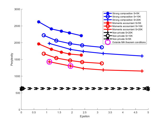
Figure 1: Epsilon versus perplexity, varying $\sigma$ and $S$, Wikipedia data, one epoch. The parameters for the two data points indicated by the pink circles do not satisfy the conditions of the moments accountant composition theorem, so those $\epsilon$ values are not formally proved.

5 Experiments using Wikipedia data

We downloaded a random $D=400,000$ documents from Wikipedia to test our algorithm. We used $50$ topics and a vocabulary set of approximately $8000$ terms. The algorithm was run for one epoch in each experiment.

We compared our moments accountant approach with a baseline method using the strong composition (Theorem 3.20 of [1]), resulting from the max divergence of the privacy loss random variable being bounded by a total budget including a slack variable $\delta$, which yields $(J\epsilon^{\prime}(e^{\epsilon^{\prime}}-1)+\sqrt{2J\log(1/\delta{{}^{\prime\prime}})}\epsilon^{\prime},\;\delta{{}^{\prime\prime}}+J\delta^{\prime})$-DP.

As our evaluation metric, we compute an upper bound on the perplexity on held-out documents. Perplexity is an information-theoretic measure of the predictive performance of probabilistic models which is commonly used in the context of language modeling [13]. The perplexity of a probabilistic model $p_{model}(x)$ on a test set of $N$ data points $x_{i}$ (e.g. words in a corpus) is defined as

$$\mbox{perplexity}(\mathcal{D}^{test},\mathbf{\bm{\lambda}})\leq\exp\left[-\left(\sum_{i}\langle\log p(\mathbf{n}^{test},\mathbf{\bm{\theta}}_{i},\mathbf{z}_{i}|\mathbf{\bm{\lambda}})\rangle_{q(\mathbf{\bm{\theta}}_{i},\mathbf{z}_{i})}-\langle\log q(\mathbf{\bm{\theta}},\mathbf{z})\rangle_{q(\mathbf{\bm{\theta}},\mathbf{z})}\right)/\sum_{i,n}\mathbf{n}_{i,n}^{test}\right],$$

where $\mathbf{n}_{i}^{test}$ is a vector of word counts for the $i$th document, $\mathbf{n}^{test}=\{\mathbf{n}_{i}^{test}\}_{i=1}^{I}$. In the above, we use the $\mathbf{\bm{\lambda}}$ that was calculated during training. We compute the posteriors over $\mathbf{z}$ and $\mathbf{\bm{\theta}}$ by performing the first step in our algorithm using the test data and the perturbed sufficient statistics we obtain during training. We adapted the python implementation by the authors of [14] for our experiments.

Figure 1 shows the trade-off between $\epsilon$ and per-word perplexity on the Wikipedia dataset for the different methods under a variety of conditions, in which we varied the value of $\sigma\in\{1.0,1.1,1.24,1.5,2\}$ and the minibatch size $S\in\{5,000,10,000,20,000\}$. We found that the moments accountant composition substantially outperformed strong composition in each of these settings. Here, we used relatively large minibatches, which were necessary to control the signal-to-noise ratio in order to obtain reasonable results for private LDA. Larger minibatches thus had lower perplexity. However, due to its impact on the subsampling rate, increasing $S$ comes at the cost of a higher $\epsilon$ for a fixed number of documents processed (in our case, one epoch). The minibatch size $S$ is limited by the conditions of the moments accountant composition theorem shown by [10], with the largest valid value being obtained at around $S\approx 20,000$ for the small noise regime where $\sigma\approx 1$.

In Table 1, for each method, we show the top $10$ words in terms of assigned probabilities for $3$ example topics. Non-private LDA results in the most coherent words among all the methods. For the private LDA models with a total privacy budget $\epsilon=2.44$ ($S=20,000,\sigma=1.24$), as we move from moments accountant to strong composition, the amount of noise added gets larger, and the topics become less coherent. We also observe that the probability mass assigned to the most probable words decreases with the noise, and thus strong composition gave less probability to the top words compared to the other methods.

Table 1: Posterior topics from private ($\epsilon=2.44$) and non-private LDA

Non-private		Moments Acc.		Strong Comp.
topic 33:		topic 33:		topic 33:
german	0.0244	function	0.0019	resolution	0.0003
system	0.0160	domain	0.0017	northward	0.0003
group	0.0109	german	0.0011	deeply	0.0003
based	0.0089	windows	0.0011	messages	0.0003
science	0.0077	software	0.0010	research	0.0003
systems	0.0076	band	0.0007	dark	0.0003
computer	0.0072	mir	0.0006	river	0.0003
software	0.0071	product	0.0006	superstition	0.0003
space	0.0061	resolution	0.0006	don	0.0003
power	0.0060	identity	0.0005	found	0.0003
topic 35:		topic 35:		topic 35:
station	0.0846	station	0.0318	station	0.0118
line	0.0508	line	0.0195	line	0.0063
railway	0.0393	railway	0.0149	railway	0.0055
opened	0.0230	opened	0.0074	opened	0.0022
services	0.0187	services	0.0064	services	0.0015
located	0.0163	closed	0.0056	stations	0.0015
closed	0.0159	code	0.0054	closed	0.0014
owned	0.0158	country	0.0052	section	0.0013
stations	0.0122	located	0.0051	platform	0.0012
platform	0.0109	stations	0.0051	company	0.0010
topic 37:		topic 37:		topic 37:
born	0.1976	born	0.0139	born	0.0007
american	0.0650	people	0.0096	american	0.0006
people	0.0572	notable	0.0092	street	0.0006
summer	0.0484	american	0.0075	charles	0.0004
notable	0.0447	name	0.0031	said	0.0004
canadian	0.0200	mountain	0.0026	events	0.0004
event	0.0170	japanese	0.0025	people	0.0003
writer	0.0141	fort	0.0025	station	0.0003
dutch	0.0131	character	0.0019	written	0.0003
actor	0.0121	actor	0.0014	point	0.0003

6 Conclusion

We have developed a practical privacy-preserving topic modeling algorithm which outputs accurate and privatized expected sufficient statistics and expected natural parameters. Our approach uses the moments accountant analysis combined with the privacy amplification effect due to subsampling of data, which significantly decrease the amount of additive noise for the same expected privacy guarantee compared to the standard analysis.

References

• [1] Cynthia Dwork and Aaron Roth. The algorithmic foundations of differential privacy. Found. Trends Theor. Comput. Sci., 9:211โ€“407, August 2014.
• [2] Cynthia Dwork, Frank McSherry, Kobbi Nissim, and Adam Smith. Calibrating noise to sensitivity in private data analysis. In Theory of Cryptography Conference, pages 265โ€“284. Springer, 2006.
• [3] M.ย J. Beal. Variational Algorithms for Approximate Bayesian Inference. PhD thesis, Gatsby Unit, University College London, 2003.
• [4] Mijung Park, Jamesย R. Foulds, Kamalika Chaudhuri, and Max Welling. DP-EM: Differentially private expectation maximization. In Proceedings of the 20th International Conference on Artificial Intelligence and Statistics (AISTATS), 2017.
• [5] Zuhe Zhang, Benjamin Rubinstein, and Christos Dimitrakakis. On the differential privacy of Bayesian inference. In Proceedings of the Thirtieth AAAI Conference on Artificial Intelligence (AAAI), 2016.
• [6] Christos Dimitrakakis, Blaine Nelson, Aikaterini Mitrokotsa, and Benjaminย I.P. Rubinstein. Robust and private Bayesian inference. In Algorithmic Learning Theory (ALT), pages 291โ€“305. Springer, 2014.
• [7] Jamesย R. Foulds, Joseph Geumlek, Max Welling, and Kamalika Chaudhuri. On the theory and practice of privacy-preserving Bayesian data analysis. In Proceedings of the 32nd Conference on Uncertainty in Artificial Intelligence (UAI), 2016.
• [8] Gilles Barthe, Gianย Pietro Farina, Marco Gaboardi, Emilio Jesรบsย Gallego Arias, Andy Gordon, Justin Hsu, and Pierre-Yves Strub. Differentially private Bayesian programming. In Proceedings of the 2016 ACM SIGSAC Conference on Computer and Communications Security, pages 68โ€“79. ACM, 2016.
• [9] Davidย M. Blei, Andrewย Y. Ng, and Michaelย I. Jordan. Latent Dirichlet allocation. Journal of Machine Learning Research, 3(Jan):993โ€“1022, 2003.
• [10] M.ย Abadi, A.ย Chu, I.ย Goodfellow, H.ย Brendan McMahan, I.ย Mironov, K.ย Talwar, and L.ย Zhang. Deep learning with differential privacy. In Proceedings of the 2016 ACM SIGSAC Conference on Computer and Communications Security, pages 308โ€“318. July 2016.
• [11] Cynthia Dwork, Guyย N Rothblum, and Salil Vadhan. Boosting and differential privacy. In Foundations of Computer Science (FOCS), 2010 51st Annual IEEE Symposium on, pages 51โ€“60. IEEE, 2010.
• [12] Mark Bun and Thomas Steinke. Concentrated differential privacy: Simplifications, extensions, and lower bounds. In Theory of Cryptography Conference, pages 635โ€“658. Springer, 2016.
• [13] Fred Jelinek, Robertย L Mercer, Lalitย R Bahl, and Jamesย K Baker. Perplexityโ€“a measure of the difficulty of speech recognition tasks. The Journal of the Acoustical Society of America, 62(S1):S63โ€“S63, 1977.
• [14] Matthew Hoffman, Francisย R. Bach, and Davidย M. Blei. Online learning for latent Dirichlet allocation. In J.ย D. Lafferty, C.ย K.ย I. Williams, J.ย Shawe-Taylor, R.ย S. Zemel, and A.ย Culotta, editors, Advances in Neural Information Processing Systems 23, pages 856โ€“864. Curran Associates, Inc., 2010.