Constructing Frequency Domains on Graphs in Near-Linear Time

Abstract.

Analysis of big data has become an increasingly relevant area of research, with data often represented on discrete networks both constructed and organic. While for structured domains, there exist intuitive definitions of signals and frequencies, the definitions are much less obvious for data sets associated with a given network. Often, the eigenvectors of an induced graph Laplacian are used to construct an orthogonal set of low-frequency vectors. For larger graphs, however, the computational cost of creating such structures becomes untenable, and the quality of the approximation is adequate only for signals near the span of the set. We propose a construction of a full basis of frequencies with computational complexity that is near-linear in time and linear in storage. Using this frequency domain, we can compress data sets on unstructured graphs more robustly and accurately than spectral-based constructions.

1. Introduction

Graphs provide a representation for data of interacting discrete objects in a given system. For structured data, such as an image or video, there exist extremely efficient methods for compression and storage, such as the fast Fourier transform [42] and wavelet approaches [19]. These techniques are often hailed as some of the most important and influential discoveries of the $20^{\text{th}}$ century. When dealing with unstructured data or a discrete graph (which lacks geometric foundation), the definition of a frequency becomes much less clear and the analogous techniques less obvious. This has made the area of signal processing on graphs a major research area in the $21^{\text{st}}$ century thus far.

Sometimes, the graph is a constructed representation, such as a “similarity” graph [43]. This construction is useful in areas such as spectral clustering [28, 25], data visualization [2], and dimension reduction of data [9, 3]. However, often the graph is not a construct. Instead, the natural structure from which the data comes is a pre-existing network, such as a biological [5, 24], economic [22], neurological [6], transportation [4], sensor [29], or social [27, 23] network. In what follows, we may safely ignore whether the given graph is organic or constructed. In both cases, the connectivity of the graph represents information regarding the similarity of discrete objects and, therefore, implies similarity and smoothness of the data produced by related objects.

Most often, an associated discrete Laplacian of the graph is used, and the spectrum and eigenvectors of the Laplacian are used to define a frequency domain, with the eigenspaces of minimal and maximal eigenvalues producing low- and high-pass filters, respectively [39]. This definition is intuitive; it is well known that the Fourier transform of a real-valued function on the real line is an expansion in the eigenfunctions of the continuous Laplacian. There is great debate as to which discrete Laplacian is the most suitable; the answer varies depending on which properties are deemed most important [21]. In this work, we consider the unnormalized graph Laplacian of $G=(V,E)$, denoted by $L(G)\in{\rm I\!R}^{n\times n}$, $n=|V|$, and defined by the bilinear form

(1) $$\langle L(G)u,v\rangle=\sum_{(i,j)\in E}(u_{i}-u_{j})(v_{i}-v_{j})$$

for any $u,v\in{\rm I\!R}^{n}$, though other choices, such as the normalized or random walk Laplacian, would be equally appropriate. These spectral-type frequency constructions have been studied extensively in [37, 38, 11, 12, 32], among others. Other techniques exist, such as wavelets on graphs [33, 20, 17, 31, 40], graph filterbanks [26], or aggregation-based algorithms [41]. In addition, the application of many discrete signal processing concepts to graphs was studied in [34, 36, 35, 7]. For an excellent coverage of the current innovations and projected areas of future work and research for signal processing on graphs, we refer the reader to [10].

In what follows, we use the localization properties of the graph to construct a multilevel structure of aggregations and produce a complete frequency domain with complexity that is near-linear in time and linear in storage, the first aggregation-based algorithm in the literature to do so. Our technique allows us to construct frequencies on large networks when the complexity of other methods may not be feasible. In addition, the efficient computation of a full basis of frequencies allows a much more robust representation of signals and does not rely heavily on the assumption of exclusively low-frequency data.

2. Near-Linear Time Frequency Domain Construction

Let $G=(V,E)$, $V=\{1,...,n\}$, be a given simple, connected, and undirected graph. For each vertex $i\in V$, we define its neighborhood $N(i)$ and degree $d(i)$ as

$$N(i)=\{j\in V\;|\;(i,j)\in E\},\quad d(i)=|N(i)|.$$

For $w\in{\rm I\!R}^{n}$ and $\sigma\subset\{1,\ldots,n\}$, $|\sigma|=k$, by $w_{\sigma}\in{\rm I\!R}^{n}$ and $[w]_{\sigma}\in{\rm I\!R}^{k}$, we denote the restrictions of $w$ to $\sigma$ in ${\rm I\!R}^{n}$ and ${\rm I\!R}^{k}$, respectively. We denote the subgraph of $G$ induced by vertices $U\subset V$ by $G[U]$. In what follows, the $\ell^{2}$-inner product is denoted by $\langle\cdot,\cdot\rangle$ and the standard (Euclidean) norm induced by the $\ell^{2}$-inner product is denoted by $\|\cdot\|$. An aggregation $\mathcal{A}=\{a_{1},...,a_{|\mathcal{A}|}\}$ of a graph $G=(V,E)$ is a non-overlapping partition of $V$ into connected components, namely,

1. $V=\bigcup_{a\in\mathcal{A}}a$,

2. $a\cap a^{\prime}=\emptyset$, $a,a^{\prime}\in\mathcal{A}$, $a\neq a^{\prime}$,

3. $G[a]$ connected, $a\in\mathcal{A}$.

Here, and in what follows, we will consider only aggregations $\mathcal{A}$ such that $|a|\geq 2$ for all $a\in\mathcal{A}$. We can construct such a set using a randomized augmented matching algorithm, such as Algorithm 1. Other suitable aggregation algorithms are found in [30]. When constructing an aggregation, we aim to minimize both the number of aggregates of order greater than two and the largest order of any aggregate, while using an algorithm that has complexity at worst near-linear in the size of the graph. Intuitively, for the majority of graphs, we should be able to accomplish both of these goals reasonably well. In particular, we recall a corollary of a famous result of Erdos and Renyi.

Theorem 2.1 ([16]).

Let $G_{n,m}$ be the graph with vertex set $V=\{1,...,n\}$ and edge set $E$ a random $m$-subset of $\{(i,j)|i,j\in V,i\neq j\}$. If $m\geq(\frac{1}{2}+C)n\log n$ for some fixed constant $C$, then

$$\lim_{\tiny\begin{array}[]{c}n\rightarrow\infty\\ n\text{ even}\end{array}}\mathrm{P}[G_{n,m}\text{ has a perfect matching }]=1.$$

All the experiments performed will use Algorithm 1, but we note that there does exist an algorithm for finding an approximately maximum matching in near-linear time [15].

Algorithm 1 Construct Aggregation $\mathcal{A}$

1. Set: ${\mathcal{A}}=\emptyset$, $\mathcal{S}=\emptyset$, $\mathcal{R}=V$.

2. For $i\in\mathcal{R}$, set $\mathcal{R}_{i}=\mathcal{R}\cap N(i)$.

   1. If $\mathcal{R}_{i}\neq\emptyset$, then

      1. $j=\arg\min\{d(\hat{j})\;|\;\hat{j}\in\mathcal{R}_{i}\};$

      2. update: $\mathcal{A}\leftarrow\mathcal{A}\cup\{i,j\}$, $\mathcal{R}\leftarrow\mathcal{R}\setminus\{i,j\}$,
             $d(k)\leftarrow d(k)-1$, $k\in N(i)$,
             $d(\ell)\leftarrow d(\ell)-1$, $\ell\in N(j)$;

   2. else update: $\mathcal{S}\leftarrow\mathcal{S}\cup\{i\}$, $\mathcal{R}\leftarrow\mathcal{R}\setminus\{i\}$.

3. For $i\in\mathcal{S}$,

   1. $a=\arg\min\{|b|\;|\;b\in\mathcal{A},b\cap N(i)\neq\emptyset\}$,
      $a\leftarrow a\cup\{i\}$.

For a given aggregation $\mathcal{A}$, we can define an associated graph on the aggregates, namely, $G_{\mathcal{A}}=(V_{\mathcal{A}},E_{\mathcal{A}})$, with

$$V_{\mathcal{A}}=\{1,...,|\mathcal{A}|\},$$

$$E_{\mathcal{A}}=\{(i,j)\;|\;\exists\;u\in a_{i},v\in a_{j},(u,v)\in E\}.$$

For each aggregate $a_{i}\in\mathcal{A}$, consider the eigendecomposition

(2) $$L(G[a_{i}])=Q_{a_{i}}\Lambda_{a_{i}}Q_{a_{i}}^{*},$$

with $\Lambda_{a_{i}}(j,j)\leq\Lambda_{a_{i}}(k,k)$, $j\leq k$, and $Q_{a_{i}}$ unitary. Let $Q_{\mathcal{A}}\in{\rm I\!R}^{n\times n}$ be the unitary matrix acting on $G$ whose restriction on $a_{i}$ equals $Q_{a_{i}}$, namely,

$$[Q_{\mathcal{A}}u]_{a_{i}}=Q_{a_{i}}^{*}[u]_{a_{i}},\quad\mbox{for all}\quad u\in{\rm I\!R}^{n},\quad a_{i}\in\mathcal{A}.$$

We define a partition of the set of vertices $V=V_{+}\cup V_{-}\cup V_{*}$, where

$$V_{+} = \{i\in V|\;\exists\;j\text{ s.t. }a_{j}(1)=i\},$$

$$V_{-} = \{i\in V|\;\exists\;j\text{ s.t. }a_{j}(2)=i\},$$

$$V_{*} = V\setminus[V_{+}\cup V_{-}].$$

Therefore, for a permutation $\pi:\{1:n\}\mapsto\{1:n\}$ and any $u\in{\rm I\!R}^{n}$, we have

$$\pi Q_{\mathcal{A}}u=\begin{bmatrix}u_{+}\\ u_{-}\\ u_{*}\end{bmatrix},\;u_{\pm}=[Q_{\mathcal{A}}u]_{{V}_{\pm}},\;u_{*}=[Q_{\mathcal{A}}u]_{{V}_{*}}.$$

Each entry in $u_{+}$ and $u_{-}$ is associated with a vertex of the aggregation graph $G_{\mathcal{A}}$. We then have two copies of $G_{\mathcal{A}}$, one with vertex set $V_{+}$ and the other with vertex set $V_{-}$, which allows us to repeat our aggregation procedure for the graph $G_{\mathcal{A}}$.

When $|a_{i}|=2$, which, by Theorem 2.1 and inspection of Algorithm 1, occurs the majority of the time for well-behaved graphs, we have

$$Q_{a}=\frac{1}{\sqrt{2}}\begin{bmatrix}1&1\\ 1&-1\end{bmatrix}.$$

It follows that, for a given aggregate $\mathcal{A}\ni a=\{i_{1},i_{2}\}$, the vectors $u_{+}$ and $u_{-}$ restricted to $a$ are given by the normalized sum and difference of the elements:

$$\sqrt{2}\;[u_{+}]_{a} = u_{i_{1}}+u_{i_{2}},$$

$$\sqrt{2}\;[u_{-}]_{a} = u_{i_{1}}-u_{i_{2}}.$$

We can apply this procedure recursively until we have $|\mathcal{A}_{J}|=1$ for some $J$. This results in a multilevel structure of graphs $G_{\mathcal{A}_{j}}$, aggregations $\mathcal{A}_{j}$, unitary matrices $Q_{\mathcal{A}_{j}}$, and permutations $\pi_{j}:\{1:n_{j}\}\mapsto\{1:n_{j}\}$, for $j=0,...,J$, where $n_{j}=|\mathcal{A}_{j-1}|$ is the number of aggregates on level $j-1$, $n_{0}:=n$, and each $Q_{\mathcal{A}_{j}}$ is an $n_{j}\times n_{j}$ matrix. For an illustration of this multilevel structure for a structural discretization of a Comanche helicopter, see Figure 1.

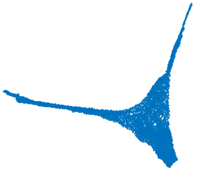
(a) Original Graph $G$

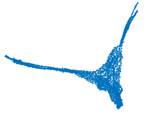
(b) Aggregation Graph $G_{\mathcal{A}_{0}}$

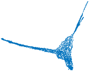
(c) Aggregation Graph $G_{\mathcal{A}_{1}}$

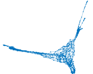
(d) Aggregation Graph $G_{\mathcal{A}_{2}}$

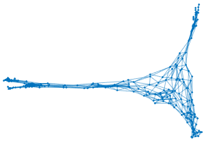
(e) Aggregation Graph $G_{\mathcal{A}_{3}}$

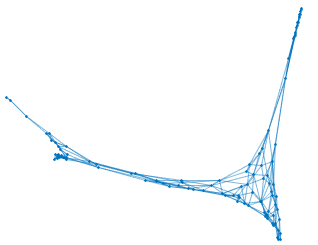
(f) Aggregation Graph $G_{\mathcal{A}_{4}}$

Figure 1. Successive application of random aggregation Algorithm 1 to a structural discretization of a Comanche helicopter. Source [13].

Let us define

$$\mathcal{Q}_{j}^{\prime}=\operatorname{diag}(\underbrace{\pi_{j}Q_{\mathcal{A}_{j}},\ldots,\pi_{j}Q_{\mathcal{A}_{j}}}_{\textstyle 2^{j}},I_{j}).$$

The matrix $I_{j}$ is the $m_{j}\times m_{j}$ identity matrix, where $m_{0}=0$, and $m_{j}=m_{j-1}+n_{j-1}-2n_{j}$, for $j=1,\ldots,J$. Let $\Pi_{j}\colon\{1:n\}\to\{1:n\}$ be a permutation such that

$$\Pi_{j}\begin{bmatrix}u_{1,+}\\ u_{1,-}\\ u_{1,*}\\ \vdots\\ \vdots\\ u_{2^{j},+}\\ u_{2^{j},-}\\ u_{2^{j},*}\\ u_{*}\end{bmatrix}=\begin{bmatrix}u_{1,+}\\ u_{1,-}\\ \vdots\\ u_{2^{j},+}\\ u_{2^{j},-}\\ u_{2^{j},*}\\ \vdots\\ u_{1,*}\\ u_{*}\end{bmatrix},\quad\parbox{164.77771pt}{for $u_{i,\pm}\in\mathbb{R}^{n_{j+1}}$, $u_{i,*}\in\mathbb{R}^{n_{j}-2n_{j+1}}$, $i=1,\dots,2^{j}$, and $u_{*}\in\mathbb{R}^{m_{j}}$.}$$

We then define

$$\mathcal{Q}_{j}=\Pi_{j}\mathcal{Q}_{j}^{\prime},\;\mathcal{Q}=\prod_{j=0}^{J}\mathcal{Q}_{J-j}.$$

By the properties of unitary matrices, $\mathcal{Q}$ is invertible, and its inverse is

$$\mathcal{Q}^{-1}=\mathcal{Q}^{*}=\prod_{j=0}^{J}\mathcal{Q}^{*}_{j}.$$

The columns of $\mathcal{Q^{*}}$ form an orthogonal basis of ${\rm I\!R}^{n}$, referred to as a basis in the frequency domain or a wavelet basis. The rationale given above is summarized in Algorithm 2.

Algorithm 2 Make Frequency Basis and Filter Signal

1. Construct aggregates and unitary matrices $\{\mathcal{A}_{i},\pi_{i}Q_{\mathcal{A}_{i}}\}_{i=0}^{J}$. Store $\{\pi_{i}Q_{\mathcal{A}_{i}}\}_{i=0}^{J}$.

2. Given signal $u\in{\rm I\!R}^{n}$, define $\widehat{u}=\prod_{i=0}^{J}\mathcal{Q}_{J-j}u$ as the frequency representation of $u$.

3. Given $k\in\{1,...,n\}$, let

   $$\sigma_{k}=\arg\max\{\|\widehat{u}_{\sigma}\|\;|\;|\sigma|=k\}.$$

   Define the $k$-frequency filter of $u$ as $v=\mathcal{Q}^{*}\widehat{u}_{\sigma_{k}}$.

In practice, the eigendecomposition in equation (2) is not computed explicitly. Instead, a dictionary of eigendecompositions for low-order graphs (e.g. $|V|\leq 5$) is stored a priori. The lookup time for this dictionary is an $O(1)$ procedure. Because the aggregate size is rarely greater than three for well-behaved graphs, this results in significantly less computation. For the remainder of the paper, we will make the following assumption:

Assumption 2.2.

There exists some constant $C_{\mathcal{A}}$, independent of $n$, such that

$$\max_{j=0,...,J}\;\max_{a\in\mathcal{A}_{j}}\;|a|\leq C_{\mathcal{A}}.$$

Of course, there exists examples for which this is not the case (e.g. the star graph $S_{n}$), but Theorem 2.1 and the experiments in Section 4 support this assumption in practice.

Once the multilevel structure has been constructed, the aggregations can be discarded and only the sparse unitary transformations need to be stored. Furthermore, the application of the local orthogonal matrices require only addition and subtraction, followed by a single normalization to the entire vector at the end of each level. Because floating point addition is typically quicker than floating point multiplication, the application of $\mathcal{Q}_{\mathcal{A}_{j}}$ is more ideal [18]. Finally, we explicitly prove the complexity and storage of Algorithm 2.

Theorem 2.3.

Algorithm 2 has complexity $O(|E|\log|V|)$ and storage $O(|V|)$.

Proof.

To verify that the algorithm is near-linear in complexity, we note that the complexity of Algorithm 1 is $O(|E|)$, and that the eigendecomposition requires at most $|V|/2$ dictionary lookups or solutions to constant sized eigenvalue problems. The structure can have at most $O(\log|V|)$ levels, each with at most half the vertices of the previous level. This gives the overall computational cost of $O(|E|\log(|E|))$. Each unitary matrix $\mathcal{Q}_{\mathcal{A}}$ has at most $C_{\mathcal{A}}|V|$ non-zero entries. This results in an overall storage cost of $O(|V|)$. ∎

2.1. An Example of Algorithm 2

In this section, on a small example we demonstrate the essential steps in Algorithm 1 and Algorithm 2. Consider the graph depicted in Fig. 2. The matching algorithm Algorithm 1 starts with a graph $G$. The vertices of $G$ are grouped by matching and they form a new graph $G_{\mathcal{A}_{0}}$. Next, the graph $G_{\mathcal{A}_{1}}$ is generated, and we continue until a graph $G_{\mathcal{A}_{2}}$ with only one vertex is generated. Note that lines decorated with springs are those chosen in the initial pairwise matching and the lines with small segments are those added for isolated points.

After the matching is available, we compute the matrices $Q_{j}$ (constructed in Algorithm 2) as follows.

$G$

$G_{\mathcal{A}_{0}}$

$G_{\mathcal{A}_{1}}$

$G_{\mathcal{A}_{2}}$

Figure 2. Matching algorithm applied on a graph

For the graph resulting from the first matching $G_{\mathcal{A}_{0}}$, the orthgonal matrices $Q_{a_{i}}$ are:

$$Q_{\{1,2\}}=Q_{\{3,4\}}=Q_{\{6,7\}}=\frac{1}{\sqrt{2}}\begin{bmatrix}1&1\\ 1&-1\end{bmatrix},$$

$$Q_{\{5,8,9\}}=\begin{bmatrix}\frac{1}{\sqrt{3}}&\frac{1}{\sqrt{2}}&\frac{1}{\sqrt{2}}\\ \frac{1}{\sqrt{3}}&0&-\frac{1}{\sqrt{2}}\\ \frac{1}{\sqrt{3}}&-\frac{1}{\sqrt{2}}&0\end{bmatrix},$$

and we have the following transformation matrix

$$Q_{\mathcal{A}_{0}}=\frac{1}{\sqrt{2}}\begin{bmatrix}1&1&0&0&0&0&0&0&0\\ 1&-1&0&0&0&0&0&0&0\\ 0&0&1&1&0&0&0&0&0\\ 0&0&1&-1&0&0&0&0&0\\ 0&0&0&0&\sqrt{\frac{2}{3}}&0&0&\sqrt{\frac{2}{3}}&\sqrt{\frac{2}{3}}\\ 0&0&0&0&0&1&1&0&0\\ 0&0&0&0&0&1&-1&0&0\\ 0&0&0&0&1&0&0&0&-1\\ 0&0&0&0&1&0&0&-1&0\end{bmatrix}.$$

The permutation which is applied to this marix is

$$\pi_{0}=\begin{pmatrix}1&2&3&4&5&6&7&8&9\\ 1&5&4&8&3&2&6&7&9\end{pmatrix}.$$

and as a result we get

$$Q_{0}=\frac{1}{\sqrt{2}}\begin{bmatrix}1&1&0&0&0&0&0&0&0\\ 0&0&0&0&0&1&1&0&0\\ 0&0&0&0&\sqrt{\frac{2}{3}}&0&0&\sqrt{\frac{2}{3}}&\sqrt{\frac{2}{3}}\\ 0&0&1&1&0&0&0&0&0\\ 1&-1&0&0&0&0&0&0&0\\ 0&0&0&0&0&1&-1&0&0\\ 0&0&0&0&1&0&0&0&-1\\ 0&0&1&-1&0&0&0&0&0\\ 0&0&0&0&1&0&0&-1&0\end{bmatrix}.$$

For the graph resulting from the second matching, $G_{\mathcal{A}_{1}}$, the matrix $Q_{1}$ has a block diagonal form, $Q_{1}=\operatorname{diag}(\pi_{1}Q_{\mathcal{A}_{1}},\pi_{1}Q_{\mathcal{A}_{1}},1)$, where

$$Q_{\mathcal{A}_{1}}=1\begin{bmatrix}1&0&1&0\\ 0&1&0&1\\ 1&0&-1&0\\ 0&1&0&-1\end{bmatrix},\quad\pi_{1}=\operatorname{id}_{\{1,2,3,4\}}.$$

Therefore, for $G_{\mathcal{A}_{2}}$, we get

$$Q_{1}=\frac{1}{\sqrt{2}}\begin{bmatrix}1&0&1&0&0&0&0&0&0\\ 0&1&0&1&0&0&0&0&0\\ 1&0&-1&0&0&0&0&0&0\\ 0&1&0&-1&0&0&0&0&0\\ 0&0&0&0&1&0&1&0&0\\ 0&0&0&0&0&1&0&1&0\\ 0&0&0&0&1&0&-1&0&0\\ 0&0&0&0&0&1&0&-1&0\\ 0&0&0&0&0&0&0&0&\sqrt{2}\end{bmatrix},\;\;Q_{2}=\frac{1}{\sqrt{2}}\begin{bmatrix}1&1&0&0&0&0&0&0&0\\ 1&-1&0&0&0&0&0&0&0\\ 0&0&1&1&0&0&0&0&0\\ 0&0&1&-1&0&0&0&0&0\\ 0&0&0&0&1&1&0&0&0\\ 0&0&0&0&1&-1&0&0&0\\ 0&0&0&0&0&0&1&1&0\\ 0&0&0&0&0&0&1&-1&0\\ 0&0&0&0&0&0&0&0&\sqrt{2}\end{bmatrix}.$$

Finally, the matrices $Q_{0}$, $Q_{1}$, and $Q_{2}$ are all constructed and ready to use for approximation of signals as in Algorithm 2.

2.2. A nonlinear version of Algorithm 2

In this subsection, we consider a nonlinear version of Algorithm 2, motived by ideas in nonlinear approximation found in DeVore [14, Section 3].

Figure 3. Hierarchy of orthonormal bases formed in constructing the frequency domain.

As it is immediately seen, Algorithm 2 produces not only a frequency basis, but a hierarchical structure which defines a hierarchy of bases (see Figure 3). The collection of all such bases is a frame for the underlying space ${\rm I\!R}^{n}$. For a given element $f\in{\rm I\!R}^{n}$ we choose expansion in a basis from this frame which has fast decay in the absolute values of the values of the coefficients in the expansion. We now explain this in more detail and refer to [14] for more general cases.

Let $\mathcal{B}:=\left\{\bm{e}_{1},\bm{e}_{2},\dots,\bm{e}_{n}\right\}$ be the natural basis of $\mathbb{R}^{n}$. We can write the matrix $(\pi Q_{\mathcal{A}})^{*}$ as

(3) $$(\pi Q_{\mathcal{A}})^{*}=\begin{bmatrix}\bm{q}_{+,1}&\cdots&\bm{q}_{+,n_{1}}&\bm{q}_{-,1}&\cdots&\bm{q}_{-,n_{1}}&\bm{q}_{*,1}&\cdots&\bm{q}_{*,n-2n_{1}}\end{bmatrix}.$$

We further define

$$\widetilde{\bm{q}}_{s+} :=\begin{bmatrix}\bm{q}_{s+,1}&\cdots&\bm{q}_{s+,n_{|s|+1}}\end{bmatrix},$$

$$\widetilde{\bm{q}}_{s-} :=\begin{bmatrix}\bm{q}_{s-,1}&\cdots&\bm{q}_{s-,n_{|s|+1}}\end{bmatrix},$$

$$\widetilde{\bm{q}}_{s*} :=\begin{bmatrix}\bm{q}_{s*,1}&\cdots&\bm{q}_{s*,n_{|s|}-2n_{|s|+1}}\end{bmatrix},$$

where $s\in\{+,-,\}^{j},j=0,\dots,J$, and $s+$, $s-$ and $s*$ are the strings obtained by appending ‘$+$’, ‘$-$’ and ‘$*$’ to $s$, respectively. Given the above notation, one can rewrite (3) as

$$(\pi Q_{\mathcal{A}})^{*}=\begin{bmatrix}\widetilde{\bm{q}}_{+}&\widetilde{\bm{q}}_{-}&\widetilde{\bm{q}}_{*}\end{bmatrix}.$$

Let $\operatorname{cols}(A)$ be the set of column vectors of a matrix $A$, and define

$$\mathcal{B}_{s+}:=\operatorname{cols}(\widetilde{\bm{q}}_{s+}),\quad\mathcal{B}_{s-}:=\operatorname{cols}(\widetilde{\bm{q}}_{s-}),\quad\mathcal{B}_{s*}:=\operatorname{cols}(\widetilde{\bm{q}}_{s*}).$$

We arrange $\mathcal{B}_{+}$, $\mathcal{B}_{-}$ and $\mathcal{B}_{*}$ as the children of the root node $\mathcal{B}$ in the tree. In a similar fashion, we recursively define

$$\begin{bmatrix}\widetilde{\bm{q}}_{s+}&\widetilde{\bm{q}}_{s-}&\widetilde{\bm{q}}_{s*}\end{bmatrix}:=\widetilde{\bm{q}}_{s}(\pi_{i}Q_{\mathcal{A}_{i}})^{*},\quad\text{for all }s\in\{+,-\}^{j},\ j=0,\dots,J.$$

Clearly, $\mathcal{B}_{s+}\cup\mathcal{B}_{s-}\cup\mathcal{B}_{s*}$ spans the same subspace of $\mathbb{R}^{n}$ as $\mathcal{B}_{s}$. In addition, given $j\in\{0,1,\dots,J\}$, the set of vectors

$$\bigcup_{s\in\{+,-,\}^{j}}(\mathcal{B}_{s+}\cup\mathcal{B}_{s-})\,\cup\,\bigcup_{i=0}^{j}\bigcup_{s\in\{+,-\}^{i}}\mathcal{B}_{s*}$$

are exactly the columns of $\left(\prod_{i=0}^{j}\mathcal{Q}_{j-i}\right)^{*}$.

The basis produced by Algorithm 2 is the specific case where $j=J$. However, we can choose an adaptive basis by taking the union of various sets $\mathcal{B}_{\cdot}$. Following [14], for a given signal $f$ on the graph, we choose the basis $\mathcal{B}^{\text{a}}$ adaptively so that the $\ell^{1}$-norm of the coefficients of $f$ in this basis

$$N(f,\mathcal{B}^{\text{a}}):=\sum_{\bm{q}\in\mathcal{B}^{\text{a}}}\lvert(f,\bm{q})\rvert$$

is minimized. We note that this guarantees coefficient decay at least as fast of that of the basis produced by Algorithm 2. We describe the minimization procedure formally in Algorithm 3.

Algorithm 3 Find the Basis that Minimizes the $\ell^{1}$-norm of Coefficients

For each $s\in\{+,-\}^{J+1}$, set $\mathcal{B}_{s}^{\text{a}}\leftarrow\mathcal{B}_{s}$.

for $j=J,J-1,\dots,0$ do

     for $s\in\{+,-\}^{j}$ do

         $\mathcal{B}_{s}^{\text{a}}\leftarrow\operatorname*{arg\,min}\left\{N(f,\mathcal{B}^{\prime})\mid\mathcal{B}^{\prime}\in\left\{\mathcal{B}_{s},\mathcal{B}_{s+}^{\text{a}}\cup\mathcal{B}_{s+}^{\text{a}}\cup\mathcal{B}_{s*}\right\}\right\}$

     end for

end for

Output the basis $\mathcal{B}^{\text{a}}\leftarrow\mathcal{B}_{\emptyset}^{\text{a}}$

In addition, we have the following complexity and storage guarantees.

Theorem 2.4.

Algorithm 3 has complexity $O(\lvert V\rvert\log\lvert V\rvert)$ and storage $\lvert V\rvert$.

Proof.

The depth of the hierarchy is at most $\log\lvert V\rvert$, within each hierarchy, a total number of $\lvert V\rvert$ inner products need to be computed for the terms $N(f,\mathcal{B}^{\prime})$. Therefore the complexity of the algorithm is $O(\lvert V\rvert\log\lvert V\rvert)$. To store the basis chosen, we only need to store one boolean value for each element in $\{+,-\}^{j}$ ($j=0,1,\dots,J$): $1$ if $\mathcal{B}_{s}$ is chosen, or $0$ if $\mathcal{B}_{s+}^{\text{a}}\cup\mathcal{B}_{s+}^{\text{a}}\cup\mathcal{B}_{s*}$ is chosen. There are $2^{J+1}-1$ such nodes, and we have $2^{J+1}\leq\lvert V\rvert$. This gives at most $\lvert V\rvert$ storage. ∎

3. Approximation of Smooth Signals

In this section, we analyze the decay of smooth signals in our frequency domain. In particular, let

$$|u|_{G,\infty}:=\max_{(i,j)\in E}|u_{i}-u_{j}|.$$

Recall, the columns of $\mathcal{Q^{*}}$ form the orthogonal basis of our frequency domain. Let $q_{i}=\prod_{j=0}^{J}\mathcal{Q}^{*}_{j}e_{i}$. For each basis element, we can associate the label

$$\phi(i):=\max\{j|n_{j}\geq i\}.$$

This naturally gives rise to a partition

$$\Phi_{j}:=\{i|\phi(i)=j\},\quad\bigcup_{j=0}^{J}\Phi_{j}=[n],\quad\Phi_{j_{1}}\cap\Phi_{j_{2}}=\emptyset,j_{1}\neq j_{2}.$$

First, we give the following lemma regarding the approximation of smooth vectors by the constant vector $\mathbf{1}:=(1,...,1)^{T}$.

Lemma 3.1.

Let $u\in{\rm I\!R}^{m}$, $m>1$. If

$$|u_{i}-u_{i+1}|\leq\alpha\quad\text{ for }i=1,...,m-1,$$

then

$$\|u\|^{2}-\frac{\langle 1_{m},u\rangle^{2}}{\langle 1_{m},1_{m}\rangle}\leq\frac{\alpha^{2}m^{3}}{12}.$$

Proof.

Let

$$u=\sum_{i=1}^{m}\alpha_{i}\hat{1}_{i},\qquad\hat{1}_{i}(j):=\left\{\begin{matrix}1\quad j\leq i\\ 0\quad j>i\end{matrix}\right.$$

Then

$$\|u\|^{2}-\frac{\langle 1_{m},u\rangle^{2}}{\langle 1_{m},1_{m}\rangle} =\left\langle\sum_{i=1}^{m}\alpha_{i}\hat{1}_{i},\sum_{i=1}^{m}\alpha_{i}\hat{1}_{i}\right\rangle-\frac{1}{m}\left\langle 1_{m},\sum_{i=1}^{m}\alpha_{i}\hat{1}_{i}\right\rangle^{2}$$

$$=\sum_{i=1}^{m}i\alpha_{i}^{2}+2\sum_{i=1}^{m-1}\sum_{j=i+1}^{m}i\alpha_{i}\alpha_{j}-\frac{1}{m}\left[\sum_{i=1}^{m}i^{2}\alpha_{i}^{2}+2\sum_{i=1}^{m-1}\sum_{j=i+1}^{m}ij\alpha_{i}\alpha_{j}\right]$$

$$=\frac{1}{m}\left[\sum_{i=1}^{m}(m-i)i\alpha_{i}^{2}+2\sum_{i=1}^{m-1}\sum_{j=i+1}^{m}(m-j)i\alpha_{i}\alpha_{j}\right]$$

$$=\frac{1}{m}\left[\sum_{i=1}^{m-1}(m-i)i\alpha_{i}^{2}+2\sum_{i=1}^{m-2}\sum_{j=i+1}^{m-1}(m-j)i\alpha_{i}\alpha_{j}\right].$$

Noting that we have $|\alpha_{i}|\leq\alpha$, $i=1,...,m-1$, the result quickly follows:

$$\|u\|^{2}-\frac{\langle 1_{m},u\rangle^{2}}{\langle 1_{m},1_{m}\rangle} \leq\frac{\alpha^{2}}{m}\left[\sum_{i=1}^{m-1}(m-i)i+2\sum_{i=1}^{m-2}\sum_{j=i+1}^{m-1}(m-j)i\right]$$

$$=\frac{\alpha^{2}}{m}\left[\frac{1}{6}(m-1)m(m+1)+\frac{1}{12}(m-2)(m-1)m(m+1)\right]$$

$$=\frac{\alpha^{2}}{12}(m-1)m(m+1)\leq\frac{\alpha^{2}m^{3}}{12}.$$

∎

We have the following result regarding the expansion of a smooth signal in the basis $\{q_{i}\}_{i=1}^{n}$.

Lemma 3.2.

$$\sum_{i\in\Phi_{k}}\langle u,q_{i}\rangle^{2}\leq\frac{n}{12}\bigg{[}\frac{C_{\mathcal{A}}^{3}}{2}\bigg{]}^{k+1}|u|^{2}_{G,\infty}.$$

Proof.

First, we will treat $\Phi_{0}$. The elements of $\Phi_{0}$ are precisely those which correspond to the sets $V_{-}$ and $V_{*}$ of $G$. We will bound the sum of the quantities $[\mathcal{Q}_{0}u](i)^{2}$, $i\in\Phi_{0}$. By Lemma 3.1, we have

$$\sum_{i\in\Phi_{0}}[\mathcal{Q}_{0}u](i)^{2} =\sum_{a_{\ell}\in\mathcal{A}_{0}}||u_{a_{\ell}}||^{2}-\frac{\langle 1_{|a_{\ell}|},u_{a_{\ell}}\rangle}{\langle 1_{|a_{\ell}|},1_{|a_{\ell}|}\rangle}$$

$$\leq\sum_{a_{\ell}\in\mathcal{A}_{0}}\frac{|u|^{2}_{G,\infty}|a_{\ell}|^{3}}{12}$$

$$\leq\frac{C_{\mathcal{A}}^{3}}{24}n|u|^{2}_{G,\infty}.$$

In addition, because each $\mathcal{Q}_{j}$ is unitary and is block diagonal with respect to the partition $\Phi_{0}$ and $[n]\backslash\Phi_{0}$, this implies that

$$\sum_{i\in\Phi_{0}}\langle u,q_{i}\rangle^{2}\leq\frac{C_{\mathcal{A}}^{3}}{24}n|u|^{2}_{G,\infty}.$$

The vector $u_{+}$ satisfies

$$|u_{+}|_{G_{\mathcal{A}_{0}},\infty}\leq|u|_{G,\infty}+\frac{2}{\sqrt{C_{\mathcal{A}}}}\sum_{i=1}^{C_{\mathcal{A}}-1}|u|_{G,\infty}i\leq C_{\mathcal{A}}^{3/2}|u|_{G,\infty}.$$

Now, proceeding by induction, for $\Phi_{k}$ we will repeat the same procedure, except we will have

$$|v_{+}|_{G_{\mathcal{A}_{k-1}},\infty}\leq C_{\mathcal{A}}^{3k/2}|u|_{G,\infty}.$$

Using Lemma 3.1 and noting that $|\mathcal{A}_{k}|\leq 2^{-(k+1)}n$, we obtain the bound

$$\sum_{i\in\Phi_{k}}\langle u,q_{i}\rangle^{2} \leq|\mathcal{A}_{k}|\bigg{[}\frac{C_{\mathcal{A}}^{3k}|u|^{2}_{G,\infty}C_{\mathcal{A}}^{3}}{12}\bigg{]}\leq\frac{n}{12}\bigg{[}\frac{C_{\mathcal{A}}^{3}}{2}\bigg{]}^{k+1}|u|^{2}_{G,\infty}.$$

∎

Based on Lemma 3.2, we can now give theoretical bounds on the quality of the $k$-term approximation $\widehat{u}_{\sigma_{k}}$, which only depends on the smoothness of the original signal and the quality of aggregation produced. We have the following theorem.

Theorem 3.3.

$$\|u-\mathcal{Q}^{*}\widehat{u_{\sigma_{k}}}\|^{2}\leq\frac{C^{3}_{\mathcal{A}}n}{12}\bigg{[}\frac{n}{k}\bigg{]}^{\log_{2}C^{3}_{\mathcal{A}}-1}|u|^{2}_{G,\infty}.$$

Proof.

$$\|u-\mathcal{Q}^{*}\widehat{u_{\sigma_{k}}}\|^{2} \leq\sum_{i=0}^{\lceil\log_{2}\frac{n}{k}\rceil-1}\frac{n}{12}\bigg{[}\frac{C_{\mathcal{A}}^{3}}{2}\bigg{]}^{i+1}|u|^{2}_{G,\infty}$$

$$\leq\frac{n}{6}\bigg{[}\frac{C_{\mathcal{A}}^{3}}{2}\bigg{]}^{\lceil\log_{2}\frac{n}{k}\rceil}|u|^{2}_{G,\infty}$$

$$\leq\frac{n}{6}\bigg{[}\frac{C_{\mathcal{A}}^{3}}{2}\bigg{]}^{\log_{2}\frac{n}{k}+1}|u|^{2}_{G,\infty}$$

$$=\frac{C^{3}_{\mathcal{A}}n}{12}\bigg{[}\frac{C_{\mathcal{A}}^{3}}{2}\bigg{]}^{\log_{2}\frac{n}{k}}|u|^{2}_{G,\infty}$$

$$=\frac{C^{3}_{\mathcal{A}}n}{12}\bigg{[}\frac{n}{k}\bigg{]}^{\log_{2}C^{3}_{\mathcal{A}}-1}|u|^{2}_{G,\infty}.$$

∎

This proves that for sufficiently smooth signals and perfect matchings, the decay in the coefficients of our frequency domain is of order at least $k^{-2}$.

4. Results and Discussion

We now consider how the complexity, storage costs and performance of Algorithm 2 for several examples.

We note that spectral-based techniques require at least $O(k|E|\log^{1/2}|V|)$ computations and $O(k|V|)$ storage to compute a $k$-dimensional low-frequency subspace, and $O(|V||E|\log^{1/2}|V|)$ computations and $O(|V|^{2})$ storage to create a full frequency domain [8]. The latter procedure is untenable for even moderately large graphs. Algorithm 2 is superior in complexity and storage for any choice of $k=\omega(\log^{1/2}|V|)$, and it produces an entire frequency domain rather than a $k$-dimensional subspace. See Table 1.

In addition, Algorithm 2 is applicable to low-pass data compression. For a given sparse network $G=(V,E)$, $n=|V|$, $|E|=|V|\log|V|$, suppose we have $m$ smooth signals $\{u^{(i)}\}_{i=1}^{m}\subset{\rm I\!R}^{n}$, with $m=n^{\alpha}$, $0<\alpha<1$. The current storage requirements for the network and the data combined are $O(|V|^{1+\alpha})$. Suppose we wish to compress this data so that the overall storage requirements are $O(|E|)$. Using a $k$-frequency low-pass filter for each $u^{(i)}$, the $m$ smooth signals can be compressed and stored using $O(k|V|^{\alpha})$ memory, not including the frequency domain and network storage. Using a spectral approach, we can only perform $O(\log|V|)$-frequency low-pass filtering. On the other hand, using Algorithm 2, we can compute the full frequency domain with only $O(|V|)$ storage. Because the network is sparse, we can safely perform $|V|^{1-\alpha}$-frequency low-pass filtering and still have storage requirements for the signals that are less than that of the graph. Therefore, although the quality of low-pass spectral frequencies is slightly superior to those of Algorithm 2, the large number of frequencies that Algorithm 2 provides results in improved and more robust compression.

Table 1. Complexity and Storage Costs of Algorithm 2 and $k$-Frequency Spectral Subspace

Costs	$k$-Spectral	Algorithm 2
Make Frequency Domain	$O(k|E|\log^{1/2}|V|)$	$O(|E|\log|V|)$
Map to/from Domain	$O(k|V|)$	$O(|V|)$
Store Frequency Domain	$O(k|V|)$	$O(|V|)$

To investigate the performance of Algorithm 2 and 3 we consider two simulations on real-world networks.

4.1. Compression of monthly precipitation data

The first example is on compressing the monthly precipitation data over Punjab, India in the rectangle $[29^{\circ}N,33^{\circ}N]\times[73.25^{\circ}E,77.5^{\circ}E]$. The original data is on $(512\times 512)$ grid. We compress the data using our compression algorithm and show how the recovered data is like compared to the original plot (Figure 4). For compressing the precipitation data, lattice graph of size $512\times 512$ is used. Figure 4 shows the plotted data over the 12 months of an year. For each month, the first plot is a plot of the original data, while the second plot is data recovered after compression using Algorithm 2. The third (most right) image shows the data recovered from the adaptive compression algorithm described in §2.2. The filtering threshold for compression is chosen to be 10,000 (out of about 260,000). In Figure 5 we plot the relative error of the compression for different filtering threshold $k$.

(a) January

(b) February

(c) March

(d) April

(e) May

(f) June

(g) July

(h) August

(i) September

(j) October

(k) November

(l) December

Figure 4. Precipitation data over 12 months from Punjab, India, in year 1980. The data were compressed and decompressed using both the original and adaptive compression algorithms.

(a) January

(b) February

(c) March

(d) April

(e) May

(f) June

(g) July

(h) August

(i) September

(j) October

(k) November

(l) December

Figure 5. Plots of relative error $\lVert u-v\rVert/\lVert u\rVert$ on the Punjab precipitation data. The horizontal axis is $\log_{2}k$, $k$ being the filtering threshold. For each plot, blue line is Algorithm 2, red line is adaptive compression.

4.2. Low pass filtering on average annual precipitation

Another example, is on low-pass filtering on average annual precipitation data for the contiguous United States in Figure 6. The spectral filter is mildly, but not notably superior to Algorithm 2.

(a) Precipitation Data

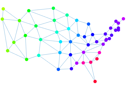
(b) Spectral Filter

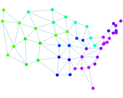
(c) Algorithm 2 Filter

Figure 6. Average annual precipitation for states in the contiguous United States, in Figure (a). Spectral filter of precipitation data, using the three minimal, nontrivial eigenvectors, in Figure (b). Algorithm 2 filter, using three component compression, in Figure (c). For both filters, signal was pre-processed with centering and normalization. Source [1].

References

• [1] I. D. A. Arguez and S. Applequist, NOAA’s U.S. climate normals (1981-2010), 2010.
• [2] G. D. Battista, P. Eades, R. Tamassia, and I. G. Tollis, Graph Drawing: Algorithms for the Visualization of Graphs, Prentice Hall PTR, Upper Saddle River, NJ, USA, 1st ed., 1998.
• [3] M. Belkin and P. Niyogi, Laplacian eigenmaps for dimensionality reduction and data representation, Neural Comput., 15 (2003), pp. 1373–1396.
• [4] M. G. H. Bell and Y. Lida, Transportation network analysis, 1997.
• [5] D. Bu, Y. Zhao, L. Cai, H. Xue, X. Zhu, H. Lu, J. Zhang, S. Sun, L. Ling, N. Zhang, G. Li, and R. Chen, Topological structure analysis of the protein–protein interaction network in budding yeast, Nucleic Acids Research, 31 (2003), pp. 2443–2450.
• [6] E. Bullmore and O. Sporns, Complex brain networks: Graph theoretical analysis of structural and functional systems, Nat Rev Neurosci, 10 (2009), pp. 186–198.
• [7] S. Chen, R. Varma, A. Sandryhaila, and J. Kovačević, Discrete signal processing on graphs: Sampling theory¡? pub _newline?, IEEE transactions on signal processing, 63 (2015), pp. 6510–6523.
• [8] M. B. Cohen, R. Kyng, G. L. Miller, J. W. Pachocki, R. Peng, A. B. Rao, and S. C. Xu, Solving sdd linear systems in nearly mlog1/2n time, in Proceedings of the 46th Annual ACM Symposium on Theory of Computing, STOC ’14, New York, NY, USA, 2014, ACM, pp. 343–352.
• [9] R. R. Coifman and S. Lafon, Diffusion maps, Applied and Computational Harmonic Analysis, 21 (2006), pp. 5 – 30. Special Issue: Diffusion Maps and Wavelets.
• [10] D. I Shuman, S. K. Narang, P. Frossard, A. Ortega, and P. Vandergheynst, The emerging field of signal processing on graphs: Extending high-dimensional data analysis to networks and other irregular domains, IEEE Signal Processing Magazine, 30 (2013), pp. 83–98.
• [11] D. I Shuman, B. Ricaud, and P. Vandergheynst, Vertex-frequency analysis on graphs, submitted to Applied and Computational Harmonic Analysis, (2013).
• [12] D. I. Shuman, C. Wiesmeyr, N. Holighaus, and P. Vandergheynst, Spectrum-adapted tight graph wavelet and vertex-frequency frames, submitted to IEEE Transactions on Signal Processing, (2013).
• [13] T. A. Davis and Y. Hu, The University of Florida sparse matrix collection, ACM Trans. Math. Softw., 38 (2011), pp. 1:1–1:25.
• [14] R. A. DeVore, Nonlinear approximation, in Acta numerica, 1998, vol. 7 of Acta Numer., Cambridge Univ. Press, Cambridge, 1998, pp. 51–150.
• [15] R. Duan and S. Pettie, Approximating maximum weight matching in near-linear time, in Foundations of Computer Science (FOCS), 2010 51st Annual IEEE Symposium on, IEEE, 2010, pp. 673–682.
• [16] P. Erdos and A. Rényi, On the existence of a factor of degree one of a connected random graph, Acta Math. Acad. Sci. Hungar, 17 (1966), pp. 359–368.
• [17] M. Gavish, B. Nadler, and R. R. Coifman, Multiscale wavelets on trees, graphs and high dimensional data: Theory and applications to semi supervised learning, in Proceedings of the 27th International Conference on Machine Learning (ICML-10), 2010, pp. 367–374.
• [18] D. Goldberg, What every computer scientist should know about floating-point arithmetic, ACM Computing Surveys (CSUR), 23 (1991), pp. 5–48.
• [19] A. Haar, Zur theorie der orthogonalen funktionensysteme, Mathematische Annalen, 69, pp. 331–371.
• [20] D. K. Hammond, P. Vandergheynst, and R. Gribonval, Wavelets on graphs via spectral graph theory, Applied and Computational Harmonic Analysis, 30 (2011), pp. 129–150.
• [21] M. Hein, J.-Y. Audibert, and U. von Luxburg, Graph Laplacians and their convergence on random neighborhood graphs, Journal of Machine Learning Research, 8 (2007), pp. 1325–1370.
• [22] M. O. Jackson et al., Social and economic networks, vol. 3, Princeton University Press, Princeton, 2008.
• [23] J. M. Kleinberg, Authoritative sources in a hyperlinked environment, Journal of the ACM (JACM), 46 (1999), pp. 604–632.
• [24] E. Lieberman, C. Hauert, and M. A. Nowak, Evolutionary dynamics on graphs, Nature, 433 (2005), pp. 312–316.
• [25] U. Luxburg, A tutorial on spectral clustering, Statistics and Computing, 17 (2007), pp. 395–416.
• [26] S. K. Narang and A. Ortega, Compact support biorthogonal wavelet filterbanks for arbitrary undirected graphs, IEEE transactions on signal processing, 61 (2013), pp. 4673–4685.
• [27] M. E. Newman, Finding community structure in networks using the eigenvectors of matrices, Physical review E, 74 (2006), p. 036104.
• [28] A. Y. Ng, M. I. Jordan, and Y. Weiss, On spectral clustering: Analysis and an algorithm, in ADVANCES IN NEURAL INFORMATION PROCESSING SYSTEMS, MIT Press, 2001, pp. 849–856.
• [29] R. Olfati-Saber and J. S. Shamma, Consensus filters for sensor networks and distributed sensor fusion, in 44th IEEE Conference on Decision and Control and 2005 European Control Conference. CDC-ECC’05, IEEE, 2005, pp. 6698–6703.
• [30] R. Rajagopalan and P. K. Varshney, Data aggregation techniques in sensor networks: A survey, Comm. Surveys and Tutorials, IEEE, 8 (2006), pp. 48–63.
• [31] I. Ram, M. Elad, and I. Cohen, Generalized tree-based wavelet transform, IEEE Transactions on Signal Processing, 59 (2011), pp. 4199–4209.
• [32] B. Ricaud, D. I. Shuman, and P. Vandergheynst, On the sparsity of wavelet coefficients for signals on graphs, in SPIE Wavelets and Sparsity, San Diego, California, August 2013.
• [33] R. Rustamov and L. J. Guibas, Wavelets on graphs via deep learning, in Advances in neural information processing systems, 2013, pp. 998–1006.
• [34] A. Sandryhaila and J. M. Moura, Discrete signal processing on graphs, IEEE transactions on signal processing, 61 (2013), pp. 1644–1656.
• [35] A. Sandryhaila and J. M. Moura, Big data analysis with signal processing on graphs: Representation and processing of massive data sets with irregular structure, IEEE Signal Processing Magazine, 31 (2014), pp. 80–90.
• [36]  , Discrete signal processing on graphs: Frequency analysis., IEEE Trans. Signal Processing, 62 (2014), pp. 3042–3054.
• [37] A. Sandryhaila and J. M. F. Moura, Discrete signal processing on graphs, IEEE Trans. Signal Processing, 61 (2013), pp. 1644–1656.
• [38] A. Sandryhaila and J. M. F. Moura, Big data analysis with signal processing on graphs: Representation and processing of massive data sets with irregular structure, IEEE Signal Processing Magazine, 31 (2014), pp. 80–90.
• [39]  , Discrete signal processing on graphs: Frequency analysis, IEEE Transactions on Signal Processing, 62 (2014), pp. 3042–3054.
• [40] N. Tremblay and P. Borgnat, Graph wavelets for multiscale community mining, IEEE Transactions on Signal Processing, 62 (2014), pp. 5227–5239.
• [41]  , Subgraph-based filterbanks for graph signals, IEEE Transactions on Signal Processing, 64 (2016), pp. 3827–3840.
• [42] S. Winograd, On computing the discrete Fourier transform, Math. Comp., 32 (1978), pp. 175–199.
• [43] Z. Wu and R. Leahy, An optimal graph theoretic approach to data clustering: Theory and its application to image segmentation, IEEE Trans. Pattern Anal. Mach. Intell., 15 (1993), pp. 1101–1113.