Diffusive estimates for random walks on
stationary random graphs of polynomial growth
Abstract
Let be a stationary random graph, and use to denote the ball of radius about in . Suppose that has annealed polynomial growth, in the sense that for some and every .
Then there is an infinite sequence of times at which the random walk on is at most diffusive: Almost surely (over the choice of ), there is a number such that
This result is new even in the case when is a stationary random subgraph of . Combined with the work of Benjamini, Duminil-Copin, Kozma, and Yadin (2015), it implies that almost surely does not admit a non-constant harmonic function of sublinear growth.
To complement this, we argue that passing to a subsequence of times is necessary, as there are stationary random graphs of (almost sure) polynomial growth where the random walk is almost surely superdiffusive at an infinite subset of times.
1 Introduction
It is a classical fact that the the standard random walk on exhibits diffusive behavior: . The well-known estimates of Varopoulos and Carne [Car85, Var85] show that, if is random walk on a graph of polynomial growth, then the speed can be at most slightly superdiffusive: , where is the graph metric on .
Kesten [Kes86] examined the distribution of the random walk on percolation clusters in . Suppose that is a stationary random subgraph of . This means that if is the random walk conditioned on with , then . Kesten’s argument can be used to show that, in this case,
| (1.1) |
On the other hand, Kesten’s approach only works for the extrinsic Euclidean metric, and not for the intrinsic metric (which can be arbitrarily larger).
Kesten asked whether (1.1) holds for any (deterministic) subgraph of . Barlow and Perkins [BP89] answered this negatively: They exhibit a subgraph of on which the Varopoulos-Carne bound is asymptotically tight (even for the Euclidean metric).
Random walk and the growth of harmonic functions
One motivation for studying situations in which Varopoulos-Carne can be improved comes from the theory of harmonic functions and their role in geometric analysis and in recent proofs of the central limit theorem for random graphs. Indeed, this led the authors of [BDCKY15] to study harmonic functions in random environments.
Consider a random rooted graph . We will assume that is locally finite and almost surely connected. Let denote the random walk conditioned on . Unless otherwise stated, we take .
Definition 1.1.
is said to be stationary if .
Let be the vertex set of , and let denote the graph metric on . For , we use the notation
The random graph has annealed polynomial growth if there exist constants such that for ,
| (1.2) |
Say that the random walk is at most diffusive if there is a constant such that
| (1.3) |
for all .
We now state the main result of [BDCKY15] for the special case of stationary random graphs. A harmonic function conditioned on is a map satisfying
Say that has sublinear growth if for every infinite sequence with , it holds that
Theorem 1.2 ([BDCKY15]).
Suppose is a stationary random graph with annealed polynomial growth, and suppose the random walk on is at most diffusive in the sense of (1.3). Then almost surely does not admit a non-constant harmonic function of sublinear growth.
Our main result is that the diffusivity assumption can be removed. Say that has weakly annealed polynomial growth if there are non-negative constants such that for ,
| (1.4) |
(Note that this is a weaker assumption than annealed polynomial growth.)
Theorem 1.3.
Suppose is a stationary random graph with weakly annealed polynomial growth. Then almost surely does not admit a non-constant harmonic function of sublinear growth.
Our proof of Theorem 1.3 proceeds in the natural way: We show that weakly annealed polynomial growth always yields a sequence of times at which the random walk is at most diffusive.
Theorem 1.4.
If is a stationary random graph of annealed polynomial growth, then for every , there is a constant and an infinite (deterministic) sequence of times such that
Note that Theorem 1.4 is new even for stationary random subgraphs of since, in contrast to Kesten’s work, we are able to bound the speed of the random walk in the intrinsic metric. To complement this result, we show that passing to a subsequence of times is necessary: There are stationary random graphs of (almost sure) polynomial growth on which the random walk is almost surely superdiffusive at an infinite subset of times.
Theorem 1.5 (See Theorem 4.1).
There is a stationary random graph of almost sure polynomial growth such that for an infinite (deterministic) sequence of times ,
We remark that instead of , one could put for any function satisfying as . This is almost tight as it nearly matches the Varopoulos-Carne estimate (see, e.g., [Woe00, Ch. 14]). Our work leaves open the intriguing question of whether whether Theorem 1.4 holds for all times when is a stationary random subgraph of .
1.1 The absence of non-constant sublinear growth harmonic functions
Let us recall that the entropy of conditioned on :
| (1.5) |
with the convention that . Similarly we define to be the entropy of the joint distribution of , conditioned on . To simplify notation, we will denote and by and , respectively.
Define the annealed entropy by
| (1.6) |
Our proof of Theorem 1.3 is based on the main result of [BDCKY15] which exploits connections between harmonic functions and the escape rate of random walk on graphs. This reduces proving Theorem 1.3 to proving the following.
Theorem 1.6.
If is a stationary random graph of weakly annealed polynomial growth, then for every , there is a constant and an infinite (deterministic) sequence of times such that and,
The proof of the preceding theorem constitutes the bulk of this article. We first show how Theorem 1.3 follows.
Proof of Theorem 1.3.
Observe that by the chain rule for entropy and stationarity of it follows that for any ,
| (1.7) |
There by Theorem 1.6, (1.7) and Fatou’s Lemma, for any , there is a constant such that with probability over the choice of , there exists an infinite sequence of times (depending on ) such that,
| (1.8) |
(for the first inequality notice ).
Suppose is harmonic on . The authors of [BDCKY15] establish the inequality: For any time ,
| (1.9) |
(This inequality is the conjunction of inequality (11) and the first inequality in the proof of Theorem 8 in [BDCKY15].)
If the graph is such that (1.8) holds and has sublinear growth, then if we consider (1.9) along the sequence and send , we conclude that almost surely
Now send to conclude that almost surely on and the random walk , we have
By stationarity, this implies almost surely for every time . Since is almost surely connected, we conclude that must be constant. Therefore Theorem 1.6 implies that almost surely does not admit a non-constant harmonic function of sublinear growth. ∎
1.2 Speed via Euclidean embeddings
Note that for discrete groups of polynomial growth, significantly stronger results than Theorem 1.4 are known (giving precise estimates on the heat kernel). See, for instance, the work of Hebisch and Saloff-Coste [HSC93]. But those estimates require detailed information about the geometry that is furnished by Gromov’s classification of such groups (in particular, they require the counting measure to be doubling). Clearly such methods are unavailable in our setting.
Even when one does not know that the counting measure is doubling, polynomial growth of a graph still yields infinitely many radii at which for some constant depending only on the growth rate. Indeed, locating such scales and performing geometric arguments that depend only on the local doubling constant underlie Kleiner’s remarkable proof of Gromov’s theorem [Kle10] (see also the quantitative results in [ST10]). (Somewhat related to the topic of the current paper, the heart of Kleiner’s argument lies in establishing that on any finitely generated group of polynomial growth, the space of harmonic functions of (fixed) polynomial growth is finite-dimensional.)
We will pursue a related course, but in order to bound the speed of the random walk after steps, we require control on the volume growth over scales, corresponding to distances in the interval . Polynomial volume growth is certainly not sufficient to find consecutive scales at which the growth is doubling (uniformly in ). Confronting this difficulty is the major technical challenge we face.
Reducing to analysis on finite subgraphs
In order to establish Theorem 1.6, we first invoke the mass transport principle to show that it suffices to examine the random walk restricted to finite subgraphs of . Let for all subsets .
In Section 3.1, we argue that it is enough to find an infinite sequence of times and radii such that the following three conditions hold for some constant :
-
1.
For every and all with ,
(1.10) -
2.
-
3.
It is noteworthy that our application of the mass transport principle uses the polynomial growth condition; specifically, we need to apply it at a scale where is doubling (see Lemma 3.1).
Embeddings and martingales
Let us focus now on condition (1) since it is the difficult one to verify. In order to control the speed of the random walk started at a uniformly random point of , we construct a family of mappings from into a Hilbert space and use the martingale methods of [NPSS06, DLP13] to derive bounds on the speed. The following statement is a slightly weaker version of Lemma 2.3 in Section 2.1.
Lemma 1.7.
Consider a graph , a finite subset , and a family of -Lipschitz mappings into a Hilbert space. Let be a given function. For , define the set of pairs
If is the stationary random walk restricted to (cf. Definition 1.12), then for every ,
| (1.11) |
where .
In Section 2.2, we show how standard tools from metric embedding theory [CKR01, KLMN05] provide a family of maps which are co-Lipschitz at a fixed scale, assuming the growth rate of balls at that scale is small.
Lemma 1.8 (Statement of Lemma 2.5).
For any graph and any , there is a -Lipschitz map such that for all , it holds that
It may help to consider now the following special case: Suppose that the counting measure on is doubling, i.e.
In that case, if we use the family from Lemma 1.8, then there is some uniformly bounded function in Lemma 1.7 such that for all . Evaluating the sum in (1.11) immediately yields , completing our verification of (1.10). (Strictly speaking, the stationary measure on and the measure restricted to are different, but they can be made arbitrarily close by taking where is chosen so that is a sufficiently good Følner set.)
In general, polynomial growth does not imply that the counting measure is doubling (and certainly the annealed form introduces even more complexity). Still, using Lemma 1.7 and Lemma 1.8 in conjunction, in Section 3.2 we show that (1.10) holds at time (for some radius ) if the average profile of growth rates of balls is sufficiently well-behaved for .
Finally, in Section 3.3, we argue that the annealed growth condition (1.4) allows us to find an infinite sequence of radii at which the average growth profile is well-behaved (with high probability over the choice of ). This is subtle, as we require control on the growth for scales (corresponding to ).111The Varopoulos-Carne bound suggests we only need control for scales corresponding to , but the same problem arises. As mentioned before, one cannot hope to find such a sequence of consecutive scales at which the volume growth is uniformly doubling. Fortunately, the subgaussian tail in (1.11) gives us some flexibility; it will suffice to find a sequence of consecutive scales where the volume growth is not increasing too fast. Once this is established, we can verify (1.10) along this sequence and confirm Theorem 1.6.
1.3 A deterministic example: Planar graphs
In this section, we present a solution to a question of Benjamini about random walks on planar graphs. It illustrates some of the ideas our main argument and their origins (in K. Ball’s notion of Markov type), as well as the reduction of speed questions to the setting of stationary Markov chains on finite subgraphs.
Consider again a graph . For a finite subset , define the edge boundary
and the edge expansion of for :
Say that is amenable if . Otherwise, say that is non-amenable.
Let denote simple random walk on . We say that the walk is ballistic if there is a constant such that for all ,
for all . Say that the walk is always somewhere at most diffusive if there is a constant such that for all ,
The following result was conjectured by Itai Benjamini.222It was made by Benjamini at the Erdös Centennial in Budapest, July, 2013 It states that for planar graphs, there are no intermediate (uniform) speeds between and .
Theorem 1.9.
Suppose that is an infinite planar graph with uniformly bounded vertex degrees. Either is amenable and the random walk is always somewhere at most diffusive, or is non-amenable and the random walk is ballistic.
Benjamini suggested this as an analog to the following dichotomy: Every amenable planar graph admits arbitrarily large sets such that , where . (This fact was announced by Gromov; see [Bow95] for a short proof.) Of course, in the non-amenable case, one has a linear isoperimetric profile: for some and every . Note that Theorem 1.9 is straightforward in the non-amenable case: If a graph is non-amenable, then has spectral radius [Kes59], hence the random walk is ballistic (see, e.g. [Woe00, Prop. 8.2]).
Remark 1.10.
If one removes the assumption of bounded degrees from Theorem 1.9, then for amenable, it still holds that the random walk is always somewhere at most diffusive (the argument below does not assume any bound on the vertex degrees). But there are non-amenable planar graphs for which the random walk does not have positive speed. We refer to [LP16, Ex 6.56] for a description of the unpublished construction of Angel, Hutchcroft, Nachmias, and Ray.
For the amenable case, we recall K. Ball’s notion of Markov type [Bal92].
Definition 1.11 (Markov type).
A metric space is said to have Markov type if there is a constant such that for every , the following holds. For every reversible Markov chain on , every mapping , and every time ,
| (1.12) |
where is distributed according to the stationary measure of the chain. One denotes by the infimal constant such that the inequality holds.
Definition 1.12 (Restricted random walk).
Consider a graph , and let
denote the neighborhood of a vertex . Fix a finite subset . Denote the measure on by . We define the random walk restricted to as the following process : For , put
It is straightforward to check that is a reversible Markov chain on with stationary measure . If has law , we say that is the stationary random walk restricted to .
Definition 1.13 (Graphic Markov type).
Define the graphic Markov type constant of a graph as the infimal number such that for every finite subset and ,
where is the stationary random walk restricted to .
Lemma 1.14.
If is an amenable graph, then for every time ,
We will prove this lemma momentarily. Let us observe first that Theorem 1.9 follows immediately in conjunction with the next theorem.
Theorem 1.15 ([DLP13]).
There is a constant such that for any planar graph .
We remark that bounding (which is all that is needed to apply Lemma 1.14) is somewhat easier than bounding ; see Corollary 2.4 and the remarks thereafter.
Proof of Lemma 1.14.
Fix a subset . Let denote the stationary random walk restricted to . From the definition of graphic Markov type, for every , we have
| (1.13) |
Note that since is stationary, it holds that for all , we have . Recall that is the random walk on . If has the law of , then has the law of conditioned on the event .
In particular, we can conclude that
| (1.14) |
Hence,
| (1.15) |
where in the first line we have used the fact that holds with probability one, and in the second line we have employed the bounds (1.13) and (1.14).
Now fix a time . Since is amenable, there exists a choice of for which . In this case, from (1.15) we obtain
Thus certainly the bound holds for some fixed , concluding the proof. ∎
2 Martingales, embeddings, and growth rates
Our proof of Theorem 1.6 involves the construction of embeddings of into a Hilbert space . The embeddings give rise to a family of martingales in whose behavior can be used to control the speed of the random walk in . This section is primarily expository; we review the martingale methods of [NPSS06, DLP13] and a construction of Euclidean embeddings that reflect the local geometry of a discrete metric space at a fixed scale [CKR01, KLMN05].
2.1 Control by martingales
Consider a finite metric space . Let denote a stationary, reversible Markov chain on with the property that
| (2.1) |
Let be a normed space and for a map , define
The following result is proved in [NPSS06] (see also [LZ94]). A similar decomposition appears already in the work of Kesten [Kes86] (see the discussion in [BP89, Sec. 2]) for the special case of percolation clusters in . A stark difference is that in Kesten’s paper, the Markov chain already takes values in a subset of (and hence the map does not appear). On the other hand, this means that Kesten only bounds the speed of the walk in the ambient Euclidean metric, whereas we are interested in the speed in the intrinsic metric (which is larger, and hence harder to bound from above).
Lemma 2.1.
Then for every , there is a forward martingale and a backward martingale such that
-
1.
-
2.
For all , it holds that
For completeness we include the proof.
Proof.
Define the martingales and by and and for ,
| (2.2) | ||||
Observe that is a martingale with respect to the filtration induced on and is a martingale with respect to the filtration induced on .
Corollary 2.2.
If is a Hilbert space, then for all ,
Define the constants
| (2.4) | ||||
| (2.5) |
Lemma 2.3.
Consider a graph , a finite subset , and a family of -Lipschitz mappings into a Hilbert space. Let be a given function. For , define the set of pairs
If is the stationary random walk restricted to (cf. Definition 1.12), then for every ,
Proof.
Use that fact that for a non-negative random variable , we have to write
where in the first inequality we have used the fact that is always true. The desired bound now follows from Corollary 2.2. ∎
We remark on one straightforward (but illustrative) application of Lemma 2.3. Following [DLP13], we say that a metric space admits a threshold embedding with distortion into a Hilbert space if there is a family of -Lipschitz maps such that
| (2.6) |
It is proved in [DLP13] that if such a threshold embedding exists, then (recall the definition of Markov type from Section 1.3). Bounding the graphic Markov type is substantially easier.
Corollary 2.4.
If is a graph and admits a threshold embedding into a Hilbert space with distortion , then
Proof.
Fix a finite subset . Let denote the stationary random walk restricted to . Let be the claimed threshold embedding. Apply Lemma 2.3 to the family with , in which case . One concludes that for every ,
Using yields a similar estimate for odd times, completing the proof. ∎
On the other hand, we will not have a uniform lower bound as in (2.6) that holds for all pairs .
Volume growth
Let be a graph with vertex set . For , we recall that is the closed -ball around in the metric . Define
| (2.7) |
In the next section, we exibit a family of mappings that reflect the geometry of well at scale when is small.
Lemma 2.5.
For any , there is a -Lipschitz map such that for all , it holds that
2.2 Embeddings and growth rates
For a metric space , define . We now prove the following generalization of Lemma 2.5.
Lemma 2.6.
If is a discrete metric space, then the following holds. For any , there is a -Lipschitz mapping such that for all ,
Lemma 2.5 is a well-known result in metric embedding theory; see, e.g., [KLMN05] where a similar lemma is stated. We provide a proof here for the sake of completeness.
By a simple compactness argument, it suffices to prove Lemma 2.6 for finite, which we now assume. Given a probability space , we use to denote the Hilbert space of measureable real-valued random variables with inner product . If is a partition of , we denote by the map that sends to the unique set containing .
Lemma 2.7.
For any value and , the following holds. Let be a random partition of with the following two properties:
-
1.
Almost surely, .
-
2.
For every ,
Then there exists a -Lipschitz mapping such that for all ,
Proof.
For every , let be a sequence of i.i.d. Bernoulli random variables (independent of ).
Consider the (random) map given by
By construction, is almost surely -Lipschitz.
Now fix with . Note that by assumption (1), . Therefore
Therefore provides the desired mapping, where is the law of the random map . Note that since is finite, is finitely supported, so one can take as a finite-dimensional Hilbert space. ∎
In light of Lemma 2.5, in order to prove Lemma 2.6, it suffices to construct an appropriate random partition. To do so, we employ the method and analysis of [CKR01].
Lemma 2.8.
For every , there is a random partition satisfying the assumptions of Lemma 2.5 with and
| (2.8) |
Proof.
Suppose that and let be a uniformly random bijection. Choose uniformly at random.
Let be the random partition constructed by iteratively cutting out the balls . In other words, where
Fix a number and a point . Let denote the smallest index for which . Then we have
| (2.9) |
For , define the interval . Note that the bad event is the same as the event .
Order the points of in non-decreasing order from : . Then (2.9) yields
| (2.10) | ||||
| (2.11) | ||||
Inequality (2.10) arises from the fact that the length of is and is chosen uniformly from an interval of length and that if or , then . Finally, to confirm (2.11), note that
In particular, conditioned on , the event can only happen if is chosen first from in the permutation .
Setting as in (2.8) completes the proof. ∎
3 Diffusive estimates
In order to apply the techniques of the preceding section, we need to reduce our main diffusive estimate (Theorem 1.6) to a statement about the random walk restricted to finite subgraphs in . In Section 3.1, we use the mass transport principle to show that it suffices to control the speed of the random walk on an appropriate sequence of balls in .
In Section 3.2, we argue that this is possible, conditioned on , as long as there are good enough bounds on the average growth rate of balls , where the average is taken over the stationary measure of the random walk restricted to . Finally, in Section 3.3, we show that the weakly annealed polynomial growth property shows yields an infinite sequence of radii such that the average growth is controlled with high probability over the choice of . This allows us to complete the proof of Theorem 1.6.
3.1 The mass transport principle
We now return to the setting where is a stationary random graph with vertex set . For a subset , define .
In order to establish Theorem 1.6, we employ an unpublished result of Russ Lyons that every stationary random graph of (weakly) annealed subexponential growth is actually a reversible random graph. For completeness, we indicate a proof at the end of this section.
In particular, we can assume that satisfies a mass transport principle (see, e.g., the extensive reference [AL07] or the discussion in [BC12]): For every positive functional , it holds that
| (3.1) |
Consider an event in (depending only on the isomorphism classes of finite rooted subgraphs).
Lemma 3.1.
For any , it holds that,
Proof.
Define a mass transportation:
Observe that,
where the last line follows from the fact that . ∎
The following theorem, along with the mass transport principle, implies Theorem 1.6. Its proof occupies Section 3.2 and Section 3.3.
Theorem 3.2.
Suppose that is a stationary random graph of weakly annealed polynomial growth. Then there is a constant depending only on the growth constants of (cf. (1.4)) and an infinite (deterministic) sequence of times and radii such that the following conditions hold:
-
1.
For every and all with , it holds that,
-
2.
-
3.
We finish off this section with the proof of Theorem 1.6.
Proof of Theorem 1.6.
Fix and apply Theorem 3.2. Applying Markov’s inequality to (3) yields
We now lower bound the probability that the random walk started from the root is at most diffusive. Note that Theorem 3.2 asserts this for the majority of the points in To transfer this to the root, we use the mass transport principle.
To apply Lemma 3.1, we define the set of rooted graphs such that
for some constant which is specified below. Using Lemma 3.1 in conjunction with (1) yields
Thus by union bound,
Choosing yields that for some , and for all sufficiently large,
Therefore it holds that for all sufficiently large, and,
yielding the desired result. ∎
3.1.1 Subexponential growth and reversibility
We now prove the following unpublished result of Russ Lyons.
Recall that is stationary if where is the random walk on with . The random graph is said to be reversible if .
Theorem 3.3.
If is a stationary random graph such that
| (3.2) |
then is reversible.
This result was proved earlier in [BC12] with the additional assumption that almost surely.
Proof.
We will borrow heavily from [BC12, Ch. 4]. The reader is encouraged to consult that paper for more detailed explanations. Let and denote the laws of and , respectively. For a fixed graph and , we denote the Radon-Nikodym derivative
One can extend this to pairs which are not necessarily adjacent: Consider any path and define
This value is independent of the path between and (see [BC12, Lem. 4.2]; this is a manifestation of the fact that a cycle and its reverse have the same probability under random walk on a graph).
Note that, because of this, for pairs such that , it holds that
| (3.3) |
where and are the laws of and , respectively. (This equality only makes sense up to sets of -measure zero.)
One has , and moreover Jensen’s inequality shows that
| (3.4) |
Let denote the set of isomorphism classes of bi-rooted graphs. Then for any Borel set and , stationarity yields
| (3.5) |
Let denote the -step transition kernel in . Using (3.5) in (3.3) implies that almost surely:
| (3.6) |
Therefore almost surely,
Note that (3.2) implies . Therefore taking expectations and again employing stationarity yields
| (3.7) |
where denotes the Shannon entropy conditioned on .
3.2 Choosing a good Følner set
Fix a rooted graph with vertex set . The most difficult part of the proof of Theorem 3.2 is verifying (1). Toward this end, we will employ Lemma 2.3 and Lemma 2.5 to control the random walk restricted to a subset of the vertices in whenever the local growth rates are sufficiently well-behaved. Consider a finite subset .
Let denote the stationary random walk restricted to (recall Definition 1.12), and let denote the corresponding stationary measure. Recall the definition of from (2.7). For , define the numbers
Note that by Markov’s inequality and a geometric summation, we have
| (3.8) |
Lemma 3.4.
For all , it holds that
| (3.9) |
Proof.
Therefore control on for yields control on the speed of . Let us define, for ,
and chose for some .
Definition 3.5 (Tempered growth).
Lemma 3.6.
For all and the following holds. If is tempered in and , then
Proof.
To see this, apply Lemma 3.4 and note that , hence
To compare the (unrestricted) random walk on to the walk restricted to , we will choose some satisfying
| (3.11) |
In particular, this implies that for ,
| (3.12) |
Definition 3.7 (Insulation).
We say that a triple is insulated in if (3.11) holds.
Our final choice of will satisfy some additional constraints, hence a complete description of the requirements is postponed to the next section. However we already have the following.
Lemma 3.8.
For every the following holds. For any rooted graph , if is tempered and insulated in , then for , it holds that
Proof.
Note that by Lemma 3.6, and Markov’s inequality,
Combining the preceding lemma with (3.11) gives us the following.
Corollary 3.9.
There is a constant such that for every if is tempered and insulated in , then
3.3 Multi-scale control of growth functionals
In this section we find scales which simultaneously satisfy all the criterion in Theorem 3.2.
We begin with the following observation. For a function , an integer , let
Then an elementary geometric summation yields
| (3.13) |
Define now the quantity
recalling that is the average of over the stationary measure of the random walk restricted to . Note that
In particular, recalling Definition 3.5,
| (3.14) |
Consider now a stationary random graph . For , define
If has weakly annealed polynomial growth (1.4), then there is a number such that
| (3.15) |
We now fix a number , and try to locate triples with that are tempered in with high probability. To ensure simultaneous occurrence of the many conditions required, we define
where
Observe that from (3.13), for any we have,
The sum in braces is bounded by which is at most . The first two terms sum telescopically to at most Putting everything together, we arrive at
| (3.16) |
Note that we use the trivial bound and the fact that .
The growth assumption (1.4) now implies that
Thus there must exist numbers with and such that
| (3.17) | ||||
| (3.18) |
and there are similarly and
| (3.19) |
such that
| (3.20) | ||||
| (3.21) |
With the above preparation, we are now ready to finish the proof of Theorem 3.2.
Proof of Theorem 3.2.
For every , we obtain a quadruple satisfying (3.17)–(3.18) and (3.20)–(3.21). Fix an infinite and strictly increasing sequence of values so that the sequence of times
is also strictly increasing.
For , define . Let denote the sequence . Inequalities (3.17) and (3.21) show that and satisfy conditions (2) and (3) of Theorem 3.2 for some constant . It remains to verify condition (1).
Toward this end, consider some . From (3.18) and (3.20), for every , we can choose constants and such that the event
has .
Define , where is the constant from Corollary 3.9. Then since , it holds that
where the first inequality uses for . Therefore,
Note that occurs for all sufficiently large (since as ).
We can thus apply Corollary 3.9 to conclude that if occurs and is sufficiently large, then there is a constant such that
We conclude that
completing the proof. ∎
4 Existence of exceptional times
We now present an example showing that one cannot hope to prove Theorem 1.6 for all times. For ease of notation, throughout this section, if is a graph, we use and for the vertex and edge set of , respectively.
Theorem 4.1.
There exists a stationary random rooted graph with the following properties:
-
1.
Almost surely: For any and it holds that
-
2.
Almost surely: .
-
3.
Let be an unbounded, monotone increasing function. Then there is a sequence of times so that
Remark 4.2.
With more effort, it is possible to obtain a similar construction with .
The basic idea of the construction is simple: Let denote the result of taking a -regular expander graph on vertices and replacing every edge by a path of length . Then by construction, the volume growth is at most quadratic, but after time , the random walk will have gone distance , making it slightly superdiffusive. The technical difficulties lie in converting this finite family of examples into a stationary random graph. To accomplish this, we build a tree of such graphs (see Figure 1(b)), with the sizes decreasing rapidly down the tree, and with buffers between the levels to enforce polynomial volume growth.
4.1 Trees of graphs

We first describe a certain way of constructing graphs from other graphs and provide some preliminary estimates on the properties of the construction. In this section, we will deal primarily with rooted graphs. For a graph , we use to denote its root.
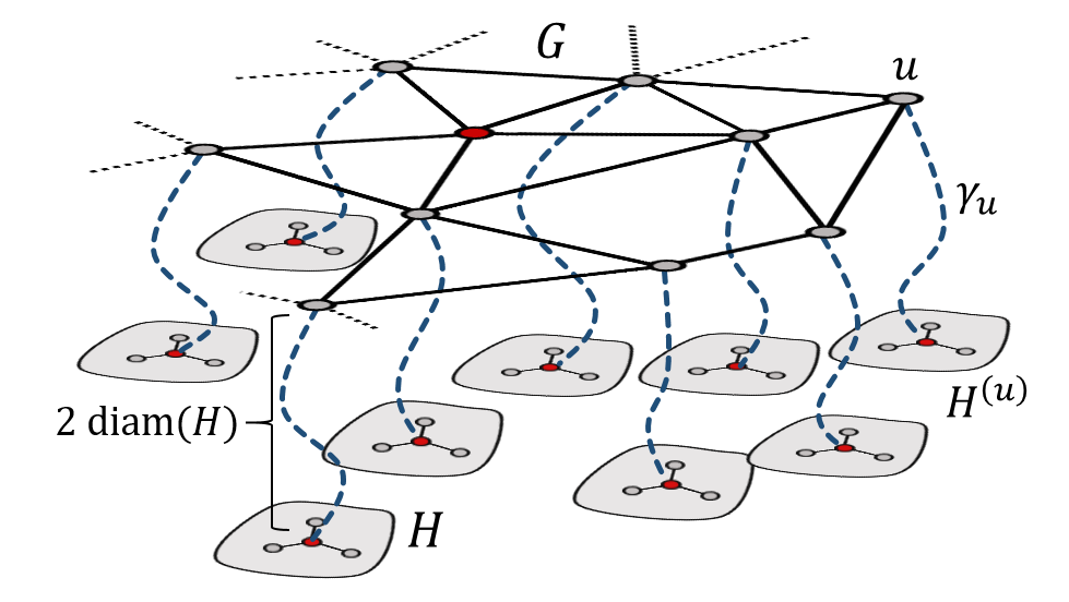
A tree of ’s under
Consider two rooted graphs and . Construct a new rooted graph as follows. Take disjoint copies of : . Let be the copy of in . Let be a collection of edge-disjoint paths of length where connects to in . Define
There is a natural identification and we define the root of . We refer to the paths as tails. See Figure 1(a).
For a graph , let us use to denote its maximum degree.
Lemma 4.3.
For any rooted graphs and and , if , then , and
Graph subdivision
For a parameter , we define a graph as the one which arises from by subdividing every edge in into a path of length . If has root , then under the natural identification , we set . Note that:
| (4.1) |
4.2 Stretched expanders and the rate of escape
Let denote a family of -regular, -vertex non-bipartite expander graphs. For each such , we distinguish an arbitrary root . We use to denote the (total variation) mixing time of a graph .
Fact 4.4.
There is a constant such that for all .
Since is -regular, a fixed vertex is further than from all but vertices in . Combining this with the preceding fact yields the following.
Lemma 4.5.
There is a constant such that the following holds for every and . If is the random walk in and , then
| (4.2) |
For a graph , define
where is the random walk on .
One has the following basic estimate (see, e.g., [LPW09, Ch. 10]):
| (4.3) |
Let denote the stationary measure of the random walk on a graph .
Lemma 4.6.
There is a constant such that the following holds for all and . Let denote the random walk on , with chosen according to the stationary measure .
Assume that and . Then for all
it holds that
Proof.
Let . Let denote the graph , but where a path of length is added between and a new copy of (so that now all vertices of have a copy of attached).
Consider the random walk on . Let be the sequence of times at which . Let (and let if no such exists). Observe that, conditioned on the sequence , the process has the law of random walk on , therefore using (4.2) yields
| (4.4) |
The waiting periods are i.i.d., and we have the estimates
Hence,
Combined with (4.4), this shows for ,
| (4.5) |
Now, note that as long as and , we can couple with the random walk on . For any ,
| (4.6) |
where the last inequality follows because is a stationary walk on , conditioned on , and because is regular.
We now require a basic estimate on . Let denote the amount of time needed for a random walk on , started at the origin, to hit the set . Then stochastically dominates , and we have the standard identities (see, e.g., [Moo73]):
Let be i.i.d. copies of , and use Chebyshev’s inequality to obtain:
For , this yields
Plugging this into (4.6) gives
Note that as long as .
4.3 The recursive construction
Observe that there is a constant such that for ,
| (4.8) |
Let us denote and suppose that for . We define an inductive sequence of rooted graphs as follows: is the graph consisting of a single vertex, and for ,
Refer to Figure 1(b) for a depiction.
We begin by consulting Lemma 4.3 for the following estimates. Using (4.8), we have for :
Thus one can easily verify by induction that
| (4.9) |
Moreover,
and one verifies by induction that for ,
| (4.10) |
From Lemma 4.3, the following bound on the vertex degrees is immediate:
| (4.11) |
Levels of vertices
The graph consists of a copy of connected to copies of via tails of length . Each such copy of contains a copy of that is connected to copies of via tails of length , and so on. If a tail connects to , we refer to it as a level- tail.
Naturally, we can think of every vertex as occurring in either in a copy of for some , or in a tail between and a copy of . Let denote the set of internal vertices in level- tails. Let denote the set of vertices occurring in some copy of . Note that the sets form a partition of .
Finally, we use the notation for the graph , together with the tail of length attached to , and the disjoint tails of length attached to all vertices of . Observe that partitions into a disjoint union of copies of with . Accordingly, we can write for the index such that is in a copy of , and for the subgraph corresponding to ’s copy of . We now observe the main point of the tails.
Lemma 4.7.
Suppose that . If , then either and lie on a common tail, or .
Lemma 4.8.
For any , , and , it holds that
Proof.
If , then
Otherwise, . ∎
Observe also the basic estimate: For ,
| (4.12) |
Lemma 4.9 (Polynomial volume growth).
For every , , and , it holds that
Proof.
Consider . The main idea is that if , then from Lemma 4.7, we know the ball cannot intersect both the top and bottom half of a level- tail unless , because the length of is at least .
Let denote the random walk on where has law .
Lemma 4.10 (Speed of the random walk).
There is a constant such that the following holds: For all and sufficiently large (with respect to ), if and
then
Proof.
For , let denote the probability that a vertex chosen uniformly at random does not fall in some copy of . First, we use (4.10) and (4.9) to bound
| (4.13) |
This yields
Observe that since , the probability that a vertex chosen from the stationary measure does not fall in some copy of is bounded by . Recall that the sequence is increasing rapidly: . Let be chosen large enough so that .
Let denote the event that lies in a copy of of . We have . Moreover, conditioned on , if the random walk avoids the root , then it can be coupled to a stationary random walk on . Now applying Lemma 4.6 with yields the desired result. ∎
4.4 Convergence to a stationary random graph
Let be chosen according to the stationary measure , and let be the law of the random rooted graph .
Lemma 4.11.
The measure exists in the local weak topology. Moreover, if has the law of , then is a stationary random graph such that, almost surely, , and for all .
Proof.
By definition of the local weak topology, to prove convergence of the measures , it suffices to show that for every , the measures converge, where is the law of . A standard application of Kolmogorov’s extension theorem then proves the existence of the limit . For more details, see [BS01].
Let denote the event that lies in a copy of . Observe that (recall (4.13)):
Suppose that occurs, and let denote the copy of in containing . In this case, we can couple and in the obvious way. Note furthermore that and are coupled (under the natural isomorphism) as long as . This yields
since . We conclude that, for fixed , it holds that
Since is summable, this yields the desired convergence as . ∎
We are ready to complete the proof of Theorem 4.1.
Proof of Theorem 4.1.
Let be the limit of constructed in Lemma 4.11. Properties (1) and (2) are satisfied by the statement of the lemma. Let denote a sequence with as and such that Lemma 4.10 applies to for .
The third property follows from Lemma 4.10 by choosing the sequence to grow fast enough so that
as . ∎
References
- [AL07] David Aldous and Russell Lyons. Processes on unimodular random networks. Electron. J. Probab., 12:no. 54, 1454–1508, 2007.
- [Bal92] K. Ball. Markov chains, Riesz transforms and Lipschitz maps. Geom. Funct. Anal., 2(2):137–172, 1992.
- [BC12] Itai Benjamini and Nicolas Curien. Ergodic theory on stationary random graphs. Electron. J. Probab., 17:no. 93, 20, 2012.
- [BDCKY15] Itai Benjamini, Hugo Duminil-Copin, Gady Kozma, and Ariel Yadin. Disorder, entropy and harmonic functions. Ann. Probab., 43(5):2332–2373, 2015.
- [Bow95] B. H. Bowditch. A short proof that a subquadratic isoperimetric inequality implies a linear one. Michigan Math. J., 42(1):103–107, 1995.
- [BP89] Martin T. Barlow and Edwin A. Perkins. Symmetric Markov chains in : how fast can they move? Probab. Theory Related Fields, 82(1):95–108, 1989.
- [BS01] Itai Benjamini and Oded Schramm. Recurrence of distributional limits of finite planar graphs. Electron. J. Probab., 6:no. 23, 13 pp. (electronic), 2001.
- [Car85] Thomas Keith Carne. A transmutation formula for Markov chains. Bull. Sci. Math. (2), 109(4):399–405, 1985.
- [CKR01] Gruia Calinescu, Howard Karloff, and Yuval Rabani. Approximation algorithms for the 0-extension problem. In Proceedings of the 12th Annual ACM-SIAM Symposium on Discrete Algorithms, pages 8–16, Philadelphia, PA, 2001.
- [DLP13] Jian Ding, James R. Lee, and Yuval Peres. Markov type and threshold embeddings. Geom. Funct. Anal., 23(4):1207–1229, 2013.
- [HSC93] W. Hebisch and L. Saloff-Coste. Gaussian estimates for Markov chains and random walks on groups. Ann. Probab., 21(2):673–709, 1993.
- [Kes59] Harry Kesten. Symmetric random walks on groups. Trans. Amer. Math. Soc., 92:336–354, 1959.
- [Kes86] Harry Kesten. Subdiffusive behavior of random walk on a random cluster. Ann. Inst. H. Poincaré Probab. Statist., 22(4):425–487, 1986.
- [Kle10] Bruce Kleiner. A new proof of Gromov’s theorem on groups of polynomial growth. J. Amer. Math. Soc., 23(3):815–829, 2010.
- [KLMN05] R. Krauthgamer, J. R. Lee, M. Mendel, and A. Naor. Measured descent: A new embedding method for finite metrics. Geom. Funct. Anal., 15(4):839–858, 2005.
- [LP16] Russell Lyons and Yuval Peres. Probability on Trees and Networks. Cambridge University Press, 2016. Available at http://pages.iu.edu/~rdlyons/.
- [LPW09] David A. Levin, Yuval Peres, and Elizabeth L. Wilmer. Markov chains and mixing times. American Mathematical Society, Providence, RI, 2009. With a chapter by James G. Propp and David B. Wilson.
- [LZ94] T. J. Lyons and T. S. Zhang. Decomposition of Dirichlet processes and its application. Ann. Probab., 22(1):494–524, 1994.
- [Moo73] J. W. Moon. Random walks on random trees. J. Austral. Math. Soc., 15:42–53, 1973.
- [NPSS06] Assaf Naor, Yuval Peres, Oded Schramm, and Scott Sheffield. Markov chains in smooth Banach spaces and Gromov-hyperbolic metric spaces. Duke Math. J., 134(1):165–197, 2006.
- [Pin94] Iosif Pinelis. Optimum bounds for the distributions of martingales in Banach spaces. Ann. Probab., 22(4):1679–1706, 1994.
- [ST10] Yehuda Shalom and Terence Tao. A finitary version of Gromov’s polynomial growth theorem. Geom. Funct. Anal., 20(6):1502–1547, 2010.
- [Var85] Nicholas Th. Varopoulos. Long range estimates for Markov chains. Bull. Sci. Math. (2), 109(3):225–252, 1985.
- [Woe00] Wolfgang Woess. Random walks on infinite graphs and groups, volume 138 of Cambridge Tracts in Mathematics. Cambridge University Press, Cambridge, 2000.