Performance of a quantum heat engine at strong reservoir coupling

Abstract

We study a quantum heat engine at strong coupling between the system and the thermal reservoirs. Exploiting a collective coordinate mapping, we incorporate system-reservoir correlations into a consistent thermodynamic analysis, thus circumventing the usual restriction to weak coupling and vanishing correlations. We apply our formalism to the example of a quantum Otto cycle, demonstrating that the performance of the engine is diminished in the strong coupling regime with respect to its weakly coupled counterpart, producing a reduced net work output and operating at a lower energy conversion efficiency. We identify costs imposed by sudden decoupling of the system and reservoirs around the cycle as being primarily responsible for the diminished performance, and define an alternative operational procedure which can partially recover the work output and efficiency. More generally, the collective coordinate mapping holds considerable promise for wider studies of thermodynamic systems beyond weak reservoir coupling.

I Introduction

Heat engines played a major role in formulating the laws of thermodynamics. For example, the second law can be understood in terms of the efficiency of an ideal Carnot cycle Carnot (1824); Blundell and Blundell (2010). Recently, significant effort has been invested into studying quantum mechanical analogues of these engines as an approach to establishing whether the same laws apply also to quantum systems; see Refs. Kosloff and Levy (2014); Gelbwaser-Klimovsky et al. (2015a); Vinjanampathy and Anders (2016); Kosloff (2013) for some contemporary reviews. Though quantum engines that have been designed to operate in standard cycles seem to respect the laws of thermodynamics Skrzypczyk et al. (2014); Scovil and Schulz-DuBois (1959); Quan et al. (2007); Kieu (2004), it has been shown that in certain situations quantum effects can be used to enhance their performance Scully et al. (2003); Scully (2002), and in some cases even violate classical thermodynamic bounds Roßnagel et al. (2014); Dillenschneider and Lutz (2009). However, these treatments usually involve circumstances beyond the scope for which the laws apply, for example non-thermal baths Roßnagel et al. (2014); Dillenschneider and Lutz (2009) or systems out of equilibrium Abah and Lutz (2014).

Typically, quantum mechanical models of heat engines are restricted to the weak coupling regime Gelbwaser-Klimovsky et al. (2013, 2015a); Kosloff and Levy (2014); Quan et al. (2007); Rezek and Kosloff (2006); Roßnagel et al. (2014); Friedenberger and Lutz (2015). That is, they assume the interaction strength between the working system and each reservoir to be negligible in comparison to their respective self-energies. During processes in which the system is coupled to a reservoir the total state may then be approximated as remaining a product state, with no correlations generated between the two. As well as significantly simplifying the analysis, this is advantageous as it makes distinguishing energy flows in terms of heat and work less problematic Seifert (2016). However, it is of both fundamental and practical importance to understand whether and how thermodynamic treatments can be modified to apply beyond such simplifying assumptions. For example, the strong coupling regime is experimentally accessible in nanoscale devices Słowik et al. (2013); Hümmer et al. (2013); Le Hur (2012); Goldstein et al. (2013); Peropadre et al. (2013); Nazir and McCutcheon (2016); Wei et al. (2014) and exciting technological implications of quantum heat machines have been proposed, such as in laser cooling Vogl and Weitz (2009); Gelbwaser-Klimovsky et al. (2015b). This motivates the requirement for a greater understanding of heat engines which operate under conditions of strong reservoir coupling .

Though considerable attention has recently been focused on identifying consistent definitions of heat, work, and internal energy in the strong coupling regime Ankerhold and Pekola (2014); Seifert (2016); Carrega et al. (2015); Esposito et al. (2015), and on formulating the second law by studying strong coupling versions of quantum fluctuation relations Campisi et al. (2009, 2011); Hanggi and Talkner (2015), or entropy and entropy production Hörhammer and Büttner (2008); Esposito et al. (2010); Deffner and Lutz (2011); Pucci et al. (2013), a consensus on a consistent approach to analysing thermodynamic cycles beyond weak reservoir coupling is arguably still lacking. In fact, there are few studies of heat engines in this regime to date, with some exceptions being Refs. Gelbwaser-Klimovsky and Aspuru-Guzik (2015); Strasberg et al. (2016); Katz and Kosloff (2016) that analyse continuously coupled engines, and Ref. Gallego et al. (2014), which considers a general work extraction process from a single temperature reservoir, rather than a full heat engine cycle.

In this article, we study a quantum heat engine operating in a discrete stroke thermodynamic (Otto) cycle between two thermal reservoirs, close in spirit to its classical counterpart, though without the usual restriction to weak reservoir coupling and vanishing system-reservoir correlations. By generalising the energetic analysis of the cycle strokes to account for both the system and reservoirs, including sudden coupling and decoupling steps, we find that strong reservoir coupling acts to diminish the engine’s performance compared to a standard weak coupling treatment. This is due primarily to the work cost incurred in turning off such interactions, which we show can be mitigated by an adiabatic decoupling procedure that partially recovers the engine’s output.

To facilitate thermodynamic calculations in the strong coupling regime we apply a collective coordinate mapping (see below). This was recently shown to predict the dynamics and equilibrium states of a quantum spin strongly coupled to a bosonic environment—the spin-boson model Leggett et al. (1987); Weiss (2012); Nitzan (2013); Breuer and Petruccione (2002); Schlosshauer (2007)—in very close agreement with accurate numerical simulations Iles-Smith et al. (2014), and also independently put forward in Ref. Strasberg et al. (2016) to analyse a continuously coupled engine. As we shall show, the collective coordinate mapping enables us to redefine the boundary between our system and its thermal reservoirs, making calculations of energy flows tractable without recourse to vastly simplifying weak coupling assumptions that neglect the generation of system-reservoir correlations. Furthermore, it allows us to retain a description in terms of reduced thermal states even within the strong coupling regime, albeit defined on an enlarged state space, such that our engine cycle calculations proceed in very close analogy to standard thermodynamic approaches.

II Otto cycle model

We shall focus on the example of a heat engine operating in an Otto cycle. Quantum Otto cycles have previously been studied in the weak coupling regime Gelbwaser-Klimovsky et al. (2015a); Kosloff and Levy (2014); Quan et al. (2007); Rezek and Kosloff (2006); Roßnagel et al. (2014); Friedenberger and Lutz (2015) with various results ranging from those analogous to classical thermodynamic bounds Quan et al. (2007), to interesting violations thereof Scovil and Schulz-DuBois (1959). An advantage of the Otto cycle is that it allows energetic changes to be distinguished by means of separate strokes where either work is extracted from (or done on) the system, or energy is exchanged between the system and the reservoirs.

We consider a quantum system with self-Hamiltonian $H_{S}$, which may be coupled to and decoupled from two heat reservoirs, one at the hot temperature $T_{h}$ and the other at the cold temperature $T_{c}$. The protocol for our Otto cycle is schematically depicted in Fig. 1. It consists of four strokes that also include system-reservoir coupling and decoupling steps:

• $A^{\prime}\rightarrow B$: At point $A^{\prime}$ the system is coupled to the hot thermal reservoir at temperature $T_{h}$ and then allowed to reach a steady state (point $B$) while its self-Hamiltonian remains fixed. The classical analogue of this stroke is referred to as the hot isochore. The system is then decoupled from the hot reservoir ($B\rightarrow B^{\prime}$). In standard treatments of the cycle, there is no energy exchange associated with the decoupling step and so it is typically ignored.

• $B^{\prime}\rightarrow C$: From point $B^{\prime}$, the system does not interact with either reservoir. Along the stroke, referred to as isentropic expansion, its self-Hamiltonian is changed from $H_{S}^{B}$ to $H_{S}^{C}$. Once at point $C$, the system is coupled to the cold reservoir, point $C^{\prime}$, ready for the next stroke.

• $C^{\prime}\rightarrow D$: At point $C^{\prime}$, the system is allowed to interact with the cold thermal reservoir at temperature $T_{c}$ and reaches a steady state (point $D$) while its self-Hamiltonian remains fixed. Classically, this stroke is referred to as the cold isochore. The system is then decoupled from the cold reservoir to reach point $D^{\prime}$.

• $D^{\prime}\rightarrow A$: From point $D^{\prime}$, the system does not interact with either reservoir. Its self-Hamiltonian is changed from $H_{S}^{D}$ ($=H_{S}^{C}$) to $H_{S}^{A}$ ($=H_{S}^{B}$) during the stroke, known as isentropic compression. The system is then coupled to the hot reservoir, reaching point $A^{\prime}$, and the cycle proceeds once more.

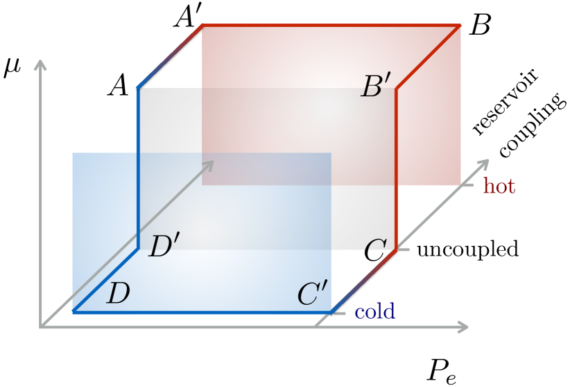
Figure 1: Quantum Otto cycle for a TLS with ground state $|g\rangle$ and excited state $|e\rangle$. The vertical axis represents the TLS splitting $\mu$ and the horizontal axis represents the population of the excited state $P_{e}$. The shaded planes indicate hot and cold reservoirs at temperatures $T_{h}$ and $T_{c}$, respectively. It is standardly a four stroke cycle: isochoric thermalisation $A^{\prime}\rightarrow B$, isentropic expansion $B^{\prime}\rightarrow C$, isochoric thermalisation $C^{\prime}\rightarrow D$, and isentropic compression $D^{\prime}\rightarrow A$. However, here we expand the cycle to explicitly include energetic contributions from coupling and decoupling the system and reservoirs: coupling to the hot reservoir $A\rightarrow A^{\prime}$, decoupling from the hot reservoir $B\rightarrow B^{\prime}$, coupling to the cold reservoir $C\rightarrow C^{\prime}$, and decoupling from the cold reservoir $D\rightarrow D^{\prime}$.

In order to perform the cycle analysis, we shall study a model consisting of a two-level system (TLS) interacting sequentially with two harmonic oscillator reservoirs, $R_{h}$ (hot) and $R_{c}$ (cold). This model, typically referred to as the spin-boson model, is paradigmatic in the study of dissipation in quantum systems Leggett et al. (1987), and has been applied to case studies such as semiconductor quantum dots, spins in magnetic fields, superconducting circuits and decoherence in biological systems Liu et al. (2015, 2014); Le Hur (2012); Goldstein et al. (2013); Peropadre et al. (2013); Nazir and McCutcheon (2016); Gullans et al. (2015); Shevchenko et al. (2010); Gilmore et al. (2005). The self-Hamiltonian for the TLS is (we set $\hbar=1$ throughout)

$$H_{S}(t)=\frac{\mu(t)}{2}I+\frac{\epsilon(t)}{2}\sigma_{z}+\frac{\Delta(t)}{2}\sigma_{x},$$ (1)

where $\epsilon(t)$ represents the TLS bias, $\Delta(t)$ the tunnelling matrix element, $\sigma_{x,z}$ denote the usual Pauli matrices, and $I$ is the identity. The eigenstates of $H_{S}$ are associated with eigenvalues $0$ and $\mu(t)$, with splitting given by

$$\mu(t)=\sqrt{\epsilon^{2}(t)+\Delta^{2}(t)}.$$ (2)

The first term in Eq. (1) thus provides a time-dependent shift of the system energy scale. Due to the periodicity of the cycle, it does not affect the work output or efficiency so that it can be chosen at will. We shall therefore use it to arrive at an unambiguous definition of positive (negative) work as that done on (by) the system during the relevant isentropic strokes.

We assume that the TLS couples to each reservoir via oscillator position, which may be expressed along with the reservoir self-Hamiltonian in the general form

$$H_{{SR}}=\sum_{k}\frac{{p_{k}}^{2}}{2m_{k}}+\frac{m_{k}{\omega_{k}}^{2}}{2}\left(x_{k}-\frac{d_{k}}{{m_{k}\omega_{k}}^{2}}\sigma_{z}\right)^{2},$$ (3)

with $d_{k}$ denoting the coupling parameters for the interaction between the spin and the bosonic field. In terms of creation and annihilation operators, Eq. (3) decomposes into a reservoir Hamiltonian and an interaction term. We define position $x^{h}_{k}=(\frac{1}{2m_{k}^{h}\omega^{h}_{k}})^{1/2}(b_{k}^{\dagger}+b_{k})$ and momentum $p^{h}_{k}=i(\frac{m_{k}^{h}\omega^{h}_{k}}{2})^{1/2}(b_{k}^{\dagger}-b_{k})$ for the hot reservoir $R_{h}$, and analogous relations for the cold reservoir $R_{c}$. The self-Hamiltonians for the reservoirs are then given by

$$H_{R_{h}} = \sum_{k}\omega^{h}_{k}(b_{k}^{\dagger}b_{k}+{1}/{2}),$$ (4)

$$H_{R_{c}} = \sum_{q}\omega^{c}_{q}(c_{q}^{\dagger}c_{q}+{1}/{2}),$$ (5)

written in terms of creation (annihilation) operators $b_{k}^{\dagger}$ $(b_{k})$ and $c_{q}^{\dagger}$ $(c_{q})$ for the hot and cold reservoir, respectively. The corresponding oscillator frequencies are denoted by $\omega^{h}_{k}$ and $\omega^{c}_{q}$. The interactions between the TLS and each reservoir, with all constants subsumed into couplings $f_{k}^{h}\equiv\frac{d_{k}}{\sqrt{m^{h}_{k}\omega^{h}_{k}}}$ and $f_{q}^{c}\equiv\frac{d_{q}}{\sqrt{m^{c}_{q}\omega^{c}_{q}}}$, may then be written

$$H_{I_{h}} = -\sigma_{z}\sum_{k}f_{k}^{h}(b_{k}^{\dagger}+b_{k})+\sum_{k}{(f_{k}^{h})}^{2}/\omega_{k}^{h},$$ (6)

$$H_{I_{c}} = -\sigma_{z}\sum_{q}f_{q}^{c}(c_{q}^{\dagger}+c_{q})+\sum_{q}{(f_{q}^{c})}^{2}/\omega_{q}^{c}.$$ (7)

The full Hamiltonian is given by the sum of all terms,

$$H(t)=H_{S}(t)+H_{R_{h}}+H_{R_{c}}+H_{I_{h}}+H_{I_{c}},$$ (8)

where it should be remembered that the interactions are only present along the relevant isochores. In the following, we shall omit terms in the reservoir and interaction Hamiltonians proportional to the identity as they do not contribute when evaluating a complete engine cycle, nor help in defining sign conventions as was the case for $H_{S}(t)$.

II.1 Reaction Coordinate Formalism

Before turning to detailed calculations of the Otto cycle performance, we review elements of the reaction (or collective) coordinate formalism that are pertinent to the analysis of a heat engine. A complete and thorough derivation of the mapping is given in Refs Iles-Smith et al. (2014, 2016).

Figure 2: Schematic of the RC mapping. Original picture (left): The TLS $S$ is strongly coupled via $f_{k}$ to an environment of harmonic oscillators $E$ with natural frequencies $\omega_{k}$. Mapped picture (right): An enlarged system $S^{\prime}$—consisting of the TLS strongly coupled via $\lambda$ to a RC with natural frequency $\Omega$—is weakly coupled via $g_{k}$ to a residual oscillator environment $E^{\prime}$ of natural frequencies $\nu_{k}$.

The reaction-coordinate (RC) approach to strong coupling is based upon a unitary mapping of the system-reservoir Hamiltonian, schematically depicted in Fig. 2. In our case, a TLS $S$ interacting with a multimode harmonic oscillator environment $E$ is mapped to an enlarged system $S^{\prime}$, consisting of the TLS and a single collective degree of freedom of the environment called the RC, which interact strongly. The RC is also weakly coupled to a redefined residual environment $E^{\prime}$, though this does not restrict the coupling strength between $S$ and $E$ in the original picture. For example, considering a single reservoir, the original Hamiltonian is given by (ignoring irrelevant terms in the reservoir and interaction Hamiltonians as stated)

$$H = \frac{\mu(t)}{2}I+\frac{\epsilon(t)}{2}\sigma_{z}+\frac{\Delta(t)}{2}\sigma_{x}+\sum_{k}\omega_{k}b_{k}^{\dagger}b_{k}$$ (9)

$$-\sigma_{z}\sum_{k}f_{k}(b_{k}^{\dagger}+b_{k}),$$

where we shall characterise the system-reservoir interaction by means of the spectral density Leggett et al. (1987)

$$J(\omega)\equiv\sum_{k}f_{k}^{2}\delta(\omega-\omega_{k}).$$ (10)

In the cycle computations, we shall take the continuum limit for the bath oscillators, and assume the following functional form of the spectral density for each reservoir,

$$J(\omega)=\frac{\alpha\omega\omega_{c}}{\omega^{2}+\omega_{c}^{2}},$$ (11)

where $\alpha$ is the coupling strength and $\omega_{c}$ is a cutoff frequency.

The mapped Hamiltonian is then obtained by defining a collective coordinate (the RC) with creation operator $a^{\dagger}=(1/\lambda)\sum_{k}f_{k}b_{k}^{\dagger}$, which satisfies bosonic commutation relations for $\lambda=\sqrt{\sum_{k}f_{k}^{2}}$, such that

$$H_{I}=-\sigma_{z}\sum_{k}f_{k}(b_{k}^{\dagger}+b_{k})=-\lambda\sigma_{z}(a^{\dagger}+a).$$ (12)

The reservoir Hamiltonian maps as

$$H_{R} =\sum_{k}\omega_{k}b_{k}^{\dagger}b_{k}$$

$$=\Omega a^{\dagger}a+\sum_{k}g_{k}(a^{\dagger}+a)(r_{k}^{\dagger}+r_{k})+\sum_{k}\nu_{k}r_{k}^{\dagger}r_{k},$$ (13)

while the system Hamiltonian remains unchanged. The full mapped Hamiltonian thus becomes 

$$\tilde{H}= \frac{\mu(t)}{2}I+\frac{\epsilon(t)}{2}\sigma_{z}+\frac{\Delta(t)}{2}\sigma_{x}-\lambda\sigma_{z}(a^{\dagger}+a)$$

$$+\Omega a^{\dagger}a+\sum_{k}g_{k}(a^{\dagger}+a)(r_{k}^{\dagger}+r_{k})+\sum_{k}\nu_{k}r_{k}^{\dagger}r_{k}.$$ (14)

Here, the RC has natural frequency $\Omega$, it couples to the system with strength $\lambda$, and to the residual environment via $g_{k}$, whose oscillator excitations at natural frequency $\nu_{k}$ are created (annihilated) by $r_{k}^{\dagger}$ ($r_{k}$). These obey bosonic commutation relations and commute with the RC operators as they describe different modes in the mapped representation. Since the residual bath is traced out when deriving a master equation for the enlarged system $S^{\prime}$, explicit expressions for the frequencies $\nu_{k}$ and the operators $r_{k}$ are not required. It suffices to find a functional form in the continuum limit for the spectral density function $\tilde{J}(\omega)\equiv\sum_{k}g_{k}^{2}\delta(\nu-\nu_{k})$ characterising the coupling between $S^{\prime}$ and the residual bath $E^{\prime}$, as well as the parameters $\Omega$ and $\lambda$, such that the Heisenberg equations of motion for the TLS are equivalent in both pictures. This results in

$$\Omega=2\pi\gamma\omega_{c},$$ (15)

$$\lambda=\sqrt{\frac{\pi\alpha\Omega}{2}},$$ (16)

and

$$\tilde{J}(\omega)=\gamma\omega e^{-{\omega}/{\Lambda}},$$ (17)

where we set the (free) parameter $\gamma=\frac{\sqrt{\epsilon^{2}+\Delta^{2}}}{2\pi\omega_{c}}$ and eventually take to infinity the cutoff frequency $\Lambda$, in order to ensure that the original form of spin-boson spectral density is still accurately represented post mapping Iles-Smith et al. (2014).

A standard Born-Markov treatment Breuer and Petruccione (2002) of the enlarged open quantum system $S^{\prime}$ now leads to a second order master equation where the strong coupling between the TLS and the RC is treated exactly, while only the weakly coupled residual environment is traced out. The master equation can be solved numerically to obtain the dynamics of the TLS (or RC) as in Refs. Iles-Smith et al. (2014, 2016), where the number of RC basis states, labelled $n$ here, is truncated at a sufficient size to ensure convergence. Benchmarking against other numerical techniques has validated that this combination of Hamiltonian mapping and second order master equation is capable of very accurately capturing both the TLS dynamics and steady-states over a wide range of parameters Iles-Smith et al. (2014, 2016), particularly when non-Markovian and strong reservoir coupling effects preclude second order (i.e. Born-Markov) expansions in the original unmapped representation. Furthermore, the mapping also allows access to properties of the reservoir through the RC itself, as well as to the system-reservoir correlations, something that is often impossible within other open systems approaches. This will in fact prove to be crucial in studying the heat engine at strong coupling in the following sections, as it allows a tractable analysis of the Otto cycle to be formulated in terms of the full system-reservoir Hamiltonian, including interactions and the resulting correlations.

Of particular importance in the present context is then the steady state solution of the master equation governing the dynamics of $S^{\prime}$, as this will determine the state of the correlated system and reservoir at the end of each isochore. Since the coupling to the residual environment is treated according to the Born-Markov approximations within the RC formalism, this steady state is given by a thermal state of the mapped system Hamiltonian

$$\tilde{H}_{S^{\prime}}\equiv\frac{\mu(t)}{2}I+\frac{\epsilon(t)}{2}\sigma_{z}+\frac{\Delta(t)}{2}\sigma_{x}-\lambda\sigma_{z}(a^{\dagger}+a)+\Omega a^{\dagger}a,$$ (18)

as

$$\tilde{\rho}_{S^{\prime}}=\frac{\exp\left(-\beta\tilde{H}_{S^{\prime}}\right)}{\textrm{tr}\left[\exp\left(-\beta\tilde{H}_{S^{\prime}}\right)\right]},$$ (19)

where $\beta=1/k_{B}T$ is the inverse temperature. The full state is then approximately

$$\tilde{\rho}\approx\tilde{\rho}_{S^{\prime}}\otimes\tilde{\rho}_{E^{\prime}}$$ (20)

where

$$\tilde{\rho}_{E^{\prime}}=\frac{\exp(-\beta\tilde{H}_{E^{\prime}})}{{\rm tr}[\exp(-\beta\tilde{H}_{E^{\prime}})]},$$ (21)

is a Gibbs thermal state of the residual environment with $\tilde{H}_{E^{\prime}}=\sum_{k}\nu_{k}r_{k}^{\dagger}r_{k}$. One can obtain the reduced state of the TLS by performing a partial trace over the RC degrees of freedom, $\rho_{S}=\textrm{tr}_{RC+E^{\prime}}[\tilde{\rho}]=\textrm{tr}_{RC}[\tilde{\rho}_{S^{\prime}}]$, which in general does not take the form of a canonical Gibbs thermal state due to the correlations generated between the system and reservoir via their non-negligible interactions. Likewise, the reduced state of the RC can be obtained from a partial trace over the TLS. Eqs. (19) and (20) are thus central to our analysis of the Otto cycle beyond weak coupling assumptions.

This can be exemplified by considering the energy expectation with respect to the full Hamiltonian

$$\langle H\rangle={\rm tr}[H\rho],$$ (22)

where $H$ is given by Eq. (9) and $\rho={\exp(-\beta H})/{{\rm tr}[\exp(-\beta H)]}$ is a thermal state of the interacting system and reservoir in the original representation. Eq. (22) is often difficult to evaluate—requiring advanced numerical techniques—without making a factorisation assumption between the system and reservoir. However, under the RC treatment it becomes

$$\langle H\rangle ={\rm tr}[\tilde{H}\tilde{\rho}]$$

$$\approx{\rm tr}[\tilde{H}_{S^{\prime}}\tilde{\rho}_{S^{\prime}}]+{\rm tr}[\tilde{H}_{E^{\prime}}\tilde{\rho}_{E^{\prime}}],$$ (23)

where in the last line we have used Eq. (20) for the mapped density operator and the fact that ${\rm tr}[\sum_{k}g_{k}(a^{\dagger}+a)(r_{k}^{\dagger}+r_{k})\tilde{\rho}_{E^{\prime}}]=0$. Thus, within the RC approach, the average energy of the interacting system and reservoir reduces to a sum of thermal expectations for the enlarged mapped system Hamiltonian and the residual bath, substantially simplifying calculations in the strong coupling regime. This is also intuitively appealing as it draws a natural boundary between the system and reservoir at finite coupling strength to link to standard thermodynamics, i.e. the residual environment provides a well defined temperature as well as a reference for energy absorption and dissipation even at strong coupling.

II.2 Generalised Otto Cycle Analysis

We shall now present a detailed analysis of the Otto cycle beyond weak system-reservoir coupling and vanishing correlations. We accomplish this by considering energetic changes with respect to the full system-reservoir Hamiltonian $H$ and state $\chi$, rather than just the internal system Hamiltonian $H_{S}$ and the reduced system state $\rho_{S}$. This leads to expressions that may be evaluated for arbitrary interaction strength using the RC formalism, and further reduce to the standard weak coupling forms under the assumption of fully factorising system-reservoir states.

II.2.1 Hot isochore

Without loss of generality, we consider starting the analysis of the cycle at point $A^{\prime}$ (see Fig. 1), when the interaction between the system and the hot reservoir has just been switched on (assumed instantaneous). The interaction with the cold reservoir is not present, however. The Hamiltonian along the isochore is given by

$$H=H_{S}^{A^{\prime}}+H_{R_{h}}+H_{R_{c}}+H_{I_{h}},$$ (24)

where

$$H_{S}^{A^{\prime}}=H_{S}^{B}=\frac{\mu_{h}}{2}I+\frac{\epsilon_{h}}{2}\sigma_{z}+\frac{\Delta_{h}}{2}\sigma_{x},$$ (25)

is unchanging along the stroke, with $H_{S}^{A^{\prime}}$ and $H_{S}^{B}$ representing the system Hamiltonian at point $A^{\prime}$ and $B$, respectively. At the end of the stroke (point $B$) the full state of the system and both reservoirs has relaxed to equilibrium, which we write as

$$\chi^{B}=\rho_{h}\otimes\rho_{R_{c}},$$ (26)

where

$$\rho_{h}=\frac{\exp\left[-\beta_{h}\left(H_{S}^{B}+H_{R_{h}}+H_{I_{h}}\right)\right]}{\textrm{tr}\left\{\exp\left[-\beta_{h}\left(H_{S}^{B}+H_{R_{h}}+H_{I_{h}}\right)\right]\right\}},$$ (27)

is the equilibrium state of the interacting TLS and hot reservoir and $\rho_{R_{c}}$ represents the state of the uncoupled cold reservoir. We have made the assumption that there are no correlations between the system and the cold reservoir at this stage in the cycle, since they are non-interacting, and hence the state $\rho_{R_{c}}$ may be factored out.

In general, $\rho_{h}$ is difficult to evaluate for a non-vanishing interaction term $H_{I_{h}}$. However, by employing the RC formalism, in particular Eq. (20), we may write

$$\rho_{h}=\frac{\exp(-\beta_{h}\tilde{H}_{S^{\prime}}^{B})}{{\rm tr}[\exp(-\beta_{h}\tilde{H}_{S^{\prime}}^{B})]}\otimes\tilde{\rho}_{E^{\prime}_{h}}=\tilde{\rho}_{S^{\prime}_{h}}\otimes\tilde{\rho}_{E^{\prime}_{h}},$$ (28)

which is far easier to calculate for finite system-reservoir coupling. Here $\tilde{\rho}_{E^{\prime}_{h}}$ is a thermal state of the hot reservoir residual environment (self Hamiltonian $\tilde{H}_{E^{\prime}_{h}}$) at inverse temperature $\beta_{h}=1/k_{B}T_{h}$ and

$$\tilde{H}_{S^{\prime}}^{B}=H_{S}^{B}-\lambda_{h}\sigma_{z}(a_{h}^{\dagger}+a_{h})+\Omega_{h}a_{h}^{\dagger}a_{h},$$ (29)

is the mapped (enlarged) system Hamiltonian including a RC for the hot reservoir.

For the cycle analysis, we are interested in the average energy at the end of the stroke, point $B$. This is obtained by taking the trace of the Hamiltonian with the full state

$$\langle H\rangle^{B} =\textrm{tr}\left[\left(H_{S}^{B}+H_{R_{h}}+H_{R_{c}}+H_{I_{h}}\right)\rho_{h}\rho_{R_{c}}\right]$$

$$=\textrm{tr}\left[\tilde{H}_{S^{\prime}}^{B}\tilde{\rho}_{S^{\prime}_{h}}\right]+\textrm{tr}\left[\tilde{H}_{E^{\prime}_{h}}\tilde{\rho}_{{E^{\prime}_{h}}}\right]+\textrm{tr}\left[H_{R_{c}}\rho_{R_{c}}\right],$$ (30)

where in the second line we have re-written the trace using the RC approach, as in Eq. (II.1). This distinguishes correlated and uncorrelated contributions due to the system and hot reservoir, the latter of which depends only on the residual thermal bath and will cancel out in the full cycle analysis. The presence of the residual thermal bath is still important, however, as it provides a reference against which we can define energy absorption along the hot isochore. The third term in Eq. (II.2.1) is the internal energy of the cold reservoir. To remain close to the spirit of the classical Otto cycle, we shall assume that the cold reservoir thermalises when uncoupled from the system, and likewise with the hot reservoir. In this way, whenever the coupling between the system and either reservoir is switched on, the reservoir is always initially in a thermal equilibrium state of well defined temperature, with correlations then generated along the subsequent isochore. It follows then that $\rho_{R_{c}}$ should be taken at this point to be a Gibbs thermal state at inverse temperature $\beta_{c}=1/k_{B}T_{c}$:

$$\rho_{R_{c}}=\rho_{th_{c}}=\frac{\exp(-\beta_{c}H_{R_{c}})}{{\rm tr}[\exp(-\beta_{c}H_{R_{c}})]}.$$ (31)

In the standard weak coupling analysis, one makes the assumption that the full state remains separable at all times with each reservoir in a thermal state at its given temperature. Under these conditions the state $\rho_{h}$ factorises into a product of the system state $\rho_{S_{h}}$ and the hot reservoir state $\rho_{th_{h}}$. Each state is of canonical Gibbs form with respect to the relevant self-Hamiltonian, which for the system reads

$$\rho_{S_{h}}=\frac{\exp\left(-\beta_{h}H_{S}^{B}\right)}{\textrm{tr}\left[\exp\left(-\beta_{h}H_{S}^{B}\right)\right]},$$ (32)

with $H_{S}^{B}$ defined in Eq. (25), and for the hot reservoir is

$$\rho_{th_{h}}=\frac{\exp(-\beta_{h}H_{R_{h}})}{{\rm tr}[\exp(-\beta_{h}H_{R_{h}})]}.$$ (33)

With the system Hamiltonian defined in equations (1) and (2), the expression for the average energy then reduces to

$$\langle H\rangle^{B}_{weak} = \frac{\mu_{h}}{2}\left[1-\tanh\left(\frac{\mu_{h}}{2k_{B}T_{h}}\right)\right]+\langle H_{R_{h}}\rangle_{th}$$ (34)

$$\>{+}\langle H_{R_{c}}\rangle_{th},$$

where we denote the reservoir thermal expectations by $\langle H_{R_{i}}\rangle_{th}={\rm tr}[H_{R_{i}}\rho_{th_{i}}]$, for $i=h,c$.

The interaction between the TLS and the hot reservoir is then switched off. In order to explicitly consider any cost associated with this step, we define the point after decoupling as $B^{\prime}$ and denote the corresponding Hamiltonian as

$$H^{B^{\prime}}=H^{B}_{S}+H_{R_{h}}+H_{R_{c}},$$ (35)

with energy

$$\langle H\rangle^{B^{\prime}}=\textrm{tr}\left[\left(H_{S}^{B}+H_{R_{h}}+H_{R_{c}}\right)\chi^{B^{\prime}}\right].$$ (36)

If $H_{I_{h}}$ is switched off instantaneously, then the full state has no time to change between points $B$ and $B^{\prime}$ and so $\chi^{B^{\prime}}=\chi^{B}=\rho_{h}\otimes\rho_{th_{c}}$, and the work in decoupling is given by

$$\langle H\rangle^{B^{\prime}}-\langle H\rangle^{B}=-\textrm{tr}\left[H_{I_{h}}\rho_{h}\right].$$ (37)

For the standard weak coupling treatment $\rho_{h}=\rho_{S_{h}}\otimes\rho_{th_{h}}$ and the energy cost equation (37) associated with decoupling from the environment evaluates identically to zero. Within the RC approach for finite coupling on the other hand, the state is given by equation (28) and we obtain

$$\langle H\rangle^{B^{\prime}}-\langle H\rangle^{B}=\lambda_{h}\textrm{tr}\left[\sigma_{z}(a_{h}^{\dagger}+a_{h})\tilde{\rho}_{S^{\prime}_{h}}\right],$$ (38)

which is generally non-zero, and the work contribution due to decoupling must therefore be included in the cycle analysis. If this contribution were negative, then we would extract work. However, we shall see that in the examples considered here it is positive, and thus represents a cost. As an alternative to attempt to mitigate this cost we also consider switching the interaction off adiabatically, the details of which are described in the Appendix.

II.2.2 Isentropic expansion

With the system now interacting with neither of the two reservoirs, the parameters in $H_{S}$ are changed such that $\mu_{h}\rightarrow\mu_{c}$, $\epsilon_{h}\rightarrow\epsilon_{c}$, $\Delta_{h}\rightarrow\Delta_{c}$. The TLS Hamiltonian at the end of the stroke (point C) becomes

$$H_{S}^{C}=\frac{\mu_{c}}{2}I+\frac{\epsilon_{c}}{2}\sigma_{z}+\frac{\Delta_{c}}{2}\sigma_{x}.$$ (39)

In the usual treatment of the Otto cycle, it is assumed that these parameters are changed slowly enough such that the quantum adiabatic theorem holds. We are then interested in the average energy along the stroke

$$\langle H(t)\rangle=\textrm{tr}\left[\left(H_{S}(t)+H_{R_{h}}+H_{R_{c}}\right)\chi(t)\right].$$ (40)

To see how the adiabatic theorem applies, one can define a unitary transformation $V\left(t\right)=\exp\left[-i\sigma_{y}{\theta\left(t\right)}/{2}\right]$, with $\theta\left(t\right)=\tan^{-1}\left[{\Delta\left(t\right)}/{\epsilon\left(t\right)}\right]$, and consider the Hamiltonian $H^{\prime}$ in the frame defined by $V(t)$. One finds

$$H^{\prime}(t) = V^{\dagger}(t)H(t)V(t)+i\dot{V}^{\dagger}(t)V(t)$$ (41)

$$= \frac{\mu(t)}{2}\left(I+\sigma_{z}\right)-\frac{\dot{\theta}(t)}{2}\sigma_{y}+H_{R_{h}}+H_{R_{c}}.$$

In the adiabatic limit, one assumes $\dot{\theta}(t)\ll 1$ and the transformation approximately diagonalises the system Hamiltonian $H_{S}(t)$. The average energy at any point along the stroke, given by equation (40), may then be calculated in this new basis:

$$\langle H(t)\rangle=\frac{\mu\left(t\right)}{2}\left\{1+\textrm{tr}\left[\sigma_{z}\chi^{\prime}(t)\right]\right\}+{\rm tr}\left[(H_{R_{h}}+H_{R_{c}})\chi(t)\right],$$ (42)

where $\chi^{\prime}(t)\equiv V^{\dagger}(t)\chi(t)V(t)$. The term $\textrm{tr}\left[\sigma_{z}\chi^{\prime}(t)\right]$ remains constant. To see this, we may substitute in for $\chi^{\prime}(t)\equiv U^{\prime}(t)\chi^{\prime}(0)U^{\prime\dagger}(t)$, where we define a time evolution operator in the transformed frame as $U^{\prime}(t)\equiv T\exp\left[-i\int_{0}^{t}H_{S}^{\prime}(\tau)d\tau\right]$, with $T$ denoting the time-ordered exponential. Thus, we have

$$\text{tr}\left[\sigma_{z}\chi^{\prime}(t)\right] = \text{tr}\left[\sigma_{z}U^{\prime}(t)\chi^{\prime}(0)U^{\prime\dagger}(t)\right]$$ (43)

$$= \text{tr}\left[U^{\prime\dagger}(t)\sigma_{z}U^{\prime}(t)\chi^{\prime}(0)\right],$$

where we have used the cyclic property of the trace. In the adiabatic limit ($\dot{\theta}\ll 1$), $H^{\prime}_{S}(t)\approx(\mu(t)/2)(I+\sigma_{z})$, such that the time evolution operator commutes with $\sigma_{z}$, and so $U^{\prime\dagger}(t)\sigma_{z}U^{\prime}(t)=\sigma_{z}$. This leaves us with

$$\text{tr}\left[\sigma_{z}\chi^{\prime}(t)\right]=\text{tr}\left[\sigma_{z}\chi^{\prime}(0)\right],$$

with the result that this term remains constant along the stroke. The average energy along the stroke is then

$$\langle H(t)\rangle =\frac{\mu(t)}{2}\left\{1+\textrm{tr}\left[\sigma_{z}\chi(0)\right]\right\}+{\rm tr}\left[(H_{R_{h}}+H_{R_{c}})\chi^{\prime}(t)\right]$$

$$=\frac{\mu(t)}{\mu(0)}\langle H_{S}(0)\rangle+{\rm tr}\left[(H_{R_{h}}+H_{R_{c}})\chi(t)\right].$$ (44)

As the reservoirs are evolving only under their own self-Hamiltonians, their energy expectations are unchanging. Hence, at the end of the stroke the energy of the system reads

$$\langle H\rangle^{C} =\textrm{tr}\left[\left(H_{S}^{C}+H_{R_{h}}+H_{R_{c}}\right)\chi^{C}\right]$$

$$=\frac{\mu_{c}}{\mu_{h}}\textrm{tr}\left[H_{S}^{B}\rho_{h}\right]+\text{tr}\left[H_{R_{h}}\rho_{h}\right]+\langle H_{R_{c}}\rangle_{th}.$$ (45)

The work extracted along the stroke is given by the difference in energy between the start and end points

$$\langle H\rangle^{C}-\langle H\rangle^{B^{\prime}}=\left(\frac{\mu_{c}}{\mu_{h}}-1\right)\textrm{tr}\left[H_{S}^{B}\rho_{h}\right],$$ (46)

which reduces in the standard weak coupling limit to

$$\langle H\rangle^{C}_{weak}-\langle H\rangle^{B^{\prime}}_{weak}=\left(\frac{\mu_{c}}{2}-\frac{\mu_{h}}{2}\right)\left[1-\tanh\left(\frac{{\mu}_{h}}{2k_{B}T_{h}}\right)\right],$$ (47)

where $\mu_{h}>\mu_{c}$.

The interaction between the system and the cold reservoir is now switched on instantaneously, leading to point $C^{\prime}$, where the energy is

$$\langle H\rangle^{C^{\prime}}=\textrm{tr}\left[\left(H_{S}^{C}+H_{R_{h}}+H_{R_{c}}+H_{I_{c}}\right)\chi^{C^{\prime}}\right],$$ (48)

and $\chi^{C^{\prime}}=\chi^{C}$. We make the assumption that the hot and cold reservoirs rapidly relax to equilibrium at temperatures $T_{h}$ and $T_{c}$ respectively, when disconnected from the system. This means that when the interaction is turned on, the system is connecting to a reservoir in a thermal equilibrium state. Hence, the work associated with coupling to the cold reservoir, $\langle H\rangle^{C^{\prime}}-\langle H\rangle^{C}$, evaluates to zero in both the weak coupling and RC treatments as the cold reservoir state $\rho_{R_{c}}$ is a thermal state at this point. Note that we do not consider the option of adiabatically turning on the coupling to the cold reservoir as this would negate the need for the cold isochore that follows, and thus has no equivalent in the standard Otto cycle.

II.2.3 Cold isochore

The system is now allowed to reach equilibrium with the cold reservoir. In analogy to the hot isochore, the full state at the end of the stroke (point $D$) is given by

$$\chi^{D}=\rho_{c}\otimes\rho_{th_{h}},$$ (49)

where

$$\rho_{c}=\frac{\exp\left[-\beta_{c}\left(H_{S}^{D}+H_{R_{c}}+H_{I_{c}}\right)\right]}{\textrm{tr}\left\{\exp\left[-\beta_{c}\left(H_{S}^{D}+H_{R_{c}}+H_{I_{c}}\right)\right]\right\}},$$ (50)

is a thermal state of the interacting TLS and cold reservoir and we assume that the hot reservoir has rethermalised along the stroke, see Eq. (33).

Employing the RC treatment to account for the interacting system and cold reservoir, the energy at point $D$ is written

$$\langle H\rangle^{D} =\textrm{tr}\left[\left(H_{S}^{C}+H_{R_{h}}+H_{R_{c}}+H_{I_{c}}\right)\rho_{c}\rho_{th_{h}}\right]$$

$$=\textrm{tr}\left[\tilde{H}_{S^{\prime}}^{C}\tilde{\rho}_{S^{\prime}_{c}}\right]+\textrm{tr}\left[\tilde{H}_{E^{\prime}_{c}}\tilde{\rho}_{E^{\prime}_{c}}\right]+\langle H_{R_{h}}\rangle_{th},$$ (51)

with

$$\rho_{c}=\frac{\exp(-\beta_{c}\tilde{H}_{S^{\prime}}^{C})}{{\rm tr}[\exp(-\beta_{c}\tilde{H}_{S^{\prime}}^{C})]}\otimes\tilde{\rho}_{E^{\prime}_{c}}=\tilde{\rho}_{S^{\prime}_{c}}\otimes\tilde{\rho}_{E^{\prime}_{c}},$$ (52)

where

$$\tilde{H}_{S^{\prime}}^{C}=H_{S}^{C}-\lambda_{c}\sigma_{z}(a_{c}^{\dagger}+a_{c})+\Omega_{c}a_{c}^{\dagger}a_{c},$$ (53)

is the RC mapped Hamiltonian for the system and cold reservoir, and $\tilde{\rho}_{E^{\prime}_{c}}$ is a thermal state of the cold reservoir residual environment (self Hamiltonian $\tilde{H}_{E^{\prime}_{c}}$) at inverse temperature $\beta_{c}$. In the weak coupling treatment, the state again reduces to the product of three thermal states for the system and the two reservoirs, such that

$$\langle H\rangle^{D}_{weak} = \frac{\mu_{c}}{2}\left[1-\tanh\left(\frac{\mu_{c}}{2k_{B}T_{c}}\right)\right]+\langle H_{R_{h}}\rangle_{th}$$ (54)

$$\>{+}\langle H_{R_{c}}\rangle_{th}.$$

In both the RC and weak coupling treatments, the energy exchanged with the cold reservoir is given by the energetic change across the isochore, $Q^{C^{\prime}D}=\langle H\rangle^{D}-\langle H\rangle^{C^{\prime}}$.

The interaction between the system and the cold reservoir is now switched off and we consider point $D^{\prime}$, where the Hamiltonian contains no interaction terms, such that

$$\langle H\rangle^{D^{\prime}}=\textrm{tr}\left[\left(H_{S}^{C}+H_{R_{h}}+H_{R_{c}}\right)\chi^{D^{\prime}}\right].$$ (55)

If the interaction is switched off instantaneously then $\chi^{D^{\prime}}=\chi^{D}=\rho_{c}\otimes\rho_{th_{h}}$, and the work cost is therefore

$$\langle H\rangle^{D^{\prime}}-\langle H\rangle^{D}=-\textrm{tr}\left[H_{I_{c}}\rho_{c}\right].$$ (56)

In the weak coupling treatment, the cold reservoir remains in a thermal state and factorises out of the expression for $\rho_{c}$, so that the cost again evaluates to zero. At strong coupling we obtain

$$\langle H\rangle^{D^{\prime}}-\langle H\rangle^{D}=\lambda_{c}\textrm{tr}\left[\sigma_{z}(a_{c}^{\dagger}+a_{c})\tilde{\rho}_{S^{\prime}_{c}}\right],$$ (57)

within the RC approach, which is generally non-zero once more. As in the hot isochore, we consider the alternative of adiabatic decoupling in the Appendix.

II.2.4 Isentropic compression

This stroke is analogous to the expansion stroke, with the system parameters changed back to their original values such that at point $A$

$$H_{S}^{A}=\frac{\mu_{h}}{2}I+\frac{\epsilon_{h}}{2}\sigma_{z}+\frac{\Delta_{h}}{2}\sigma_{x}.$$ (58)

In the adiabatic limit the energy at point $A$ is given by

$$\langle H\rangle^{A} =\textrm{tr}\left[\left(H_{S}^{A}+H_{R_{h}}+H_{R_{c}}\right)\chi^{A}\right]$$

$$=\frac{\mu_{h}}{\mu_{c}}\textrm{tr}\left[H_{S}^{C}\rho_{c}\right]+\textrm{tr}\left[H_{R_{c}}\rho_{c}\right]+\langle H_{R_{h}}\rangle_{th}.$$ (59)

The energy difference across the stroke, equivalent to the work done on the system, is

$$\langle H\rangle^{A}-\langle H\rangle^{D^{\prime}}=\left(\frac{\mu_{h}}{\mu_{c}}-1\right)\textrm{tr}\left[H_{S}^{C}\rho_{c}\right],$$ (60)

which reduces to

$$\langle H\rangle_{weak}^{A}-\langle H\rangle_{weak}^{D^{\prime}}=\left(\frac{\mu_{h}}{2}-\frac{\mu_{c}}{2}\right)\left[1-\tanh\left(\frac{\mu_{c}}{2k_{B}T_{c}}\right)\right],$$ (61)

within the weak coupling treatment. The coupling to the hot reservoir is now switched on instantaneously and we return to point $A^{\prime}$ where the Hamiltonian contains the term $H_{I_{h}}$. The energy is thus given by

$$\langle H\rangle^{A^{\prime}}= \textrm{tr}\left[(H_{S}^{B}+H_{R_{h}}+H_{R_{c}}+H_{I_{h}})\chi^{A^{\prime}}\right]$$

$$= \frac{\mu_{h}}{\mu_{c}}\textrm{tr}\left[H_{S}^{C}\rho_{c}\right]+\text{tr}\left[H_{R_{c}}\rho_{c}\right]+\langle H_{R_{h}}\rangle_{th}$$

$$= \langle H\rangle^{A},$$ (62)

where, as in the cold reservoir case, there is no cost associated with switching on the coupling to the hot reservoir.

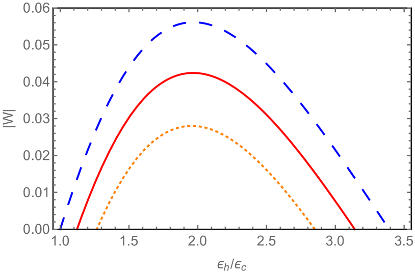
(a) (b)

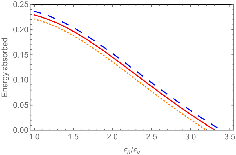
Figure 3: Adiabatic limit. Work output (a) and energy absorbed from the hot reservoir (b) for a quantum Otto cycle plotted as a function of the TLS bias at point $A$, $\epsilon_{h}$. Blue dashed curves: weak coupling; Orange dotted curves: strong coupling with instantaneous decoupling of the reservoirs; Red solid curves: strong coupling with adiabatic decoupling of the reservoirs. Parameters (in units of $\epsilon_{c}$): $\Delta_{h}=\Delta_{c}=1$, $\beta_{h}=1$, $\beta_{c}=2.5$, $\omega_{c}=2$, $\alpha=0.005$, and $n=30$ states are taken in the RC calculations.

II.3 Work output and efficiency at strong coupling

We are now in a position to evaluate the net work output and energy conversion efficiency of the strong coupling Otto cycle. The work output is obtained by summing the energetic changes along each isentropic stroke, including the work costs associated with decoupling:

$$W= W^{BB^{\prime}}+W^{B^{\prime}C}+W^{CC^{\prime}}+W^{DD^{\prime}}+W^{D^{\prime}A}+W^{AA^{\prime}}$$

$$= \left(\frac{\mu_{c}}{\mu_{h}}-1\right)\textrm{tr}\left[H_{S}^{B}\rho_{h}\right]+\left(\frac{\mu_{h}}{\mu_{c}}-1\right)\textrm{tr}\left[H_{S}^{C}\rho_{c}\right]$$

$$-\textrm{tr}\left[H_{I_{h}}\rho_{h}\right]-\textrm{tr}\left[H_{I_{c}}\rho_{c}\right].$$ (63)

Similarly, the energy transferred into the system is given by the energetic change along the hot isochore:

$$Q^{A^{\prime}B}= \langle H\rangle^{B}-\langle H\rangle^{A^{\prime}}$$

$$= \textrm{tr}\left[H_{S}^{B}\rho_{h}\right]-\frac{\mu_{h}}{\mu_{c}}\textrm{tr}\left[H_{S}^{C}\rho_{c}\right]$$

$$+\textrm{tr}\left[H_{R_{h}}\left(\rho_{h}-\rho_{th_{h}}\right)\right]+\textrm{tr}\left[H_{R_{c}}\left(\rho_{th_{c}}-\rho_{c}\right)\right]$$

$$+\textrm{tr}\left[H_{I_{h}}\rho_{h}\right].$$ (64)

In the weak coupling treatment, the reservoirs remain in thermal equilibrium such that their internal energies cancel out and the interaction terms evaluate to zero. The expressions for the net work output and energy flow from the hot reservoir then reduce to the standard forms

$$W_{weak}= \langle H\rangle^{C^{\prime}}-\langle H\rangle^{B}+\langle H\rangle^{A^{\prime}}-\langle H\rangle^{D}$$

$$= \frac{1}{2}\left(\mu_{c}-\mu_{h}\right)\left[\tanh\left(\frac{\mu_{h}}{2k_{B}T_{h}}\right)-\tanh\left(\frac{\mu_{c}}{2k_{B}T_{c}}\right)\right]$$ (65)

and

$$Q_{weak}=\frac{\mu_{h}}{2}\left[\tanh\left(\frac{\mu_{c}}{2k_{B}T_{c}}\right)-\tanh\left(\frac{\mu_{h}}{2k_{B}T_{h}}\right)\right],$$ (66)

respectively.

The efficiency of the engine is given as usual by the ratio of the net work output to the energy absorbed by the system along the hot isochore,

$$\eta=\frac{W}{Q^{A^{\prime}B}}.$$ (67)

For weak coupling this reduces to

$$\eta_{weak}=1-\frac{{\mu_{c}}}{{\mu_{h}}},$$ (68)

as expected.

III Otto cycle results

Figure 4: Adiabatic limit. Net work output of the Otto cycle split into decoupling work cost and magnitude of the remaining work extracted, plotted as a function of the TLS bias at point $A$, $\epsilon_{h}$. Blue dashed curve: weak coupling (no decoupling cost) and strong coupling work extracted ignoring work cost (adiabatic decoupling case); Orange dotted curve: strong coupling work extracted ignoring work cost (instantaneous decoupling case); Red dashed line: strong coupling cost of instantaneous decoupling; Purple solid line: strong coupling cost of adiabatic decoupling. Parameters as in Fig. 3.

We shall now present some specific examples to explore the impact of strong coupling and system-reservoir correlations on the quantum Otto engine’s performance. We begin by considering adiabatic isentropic strokes, as outlined above, though for completeness we shall subsequently extend the analysis to the opposite limit of sudden isentropes as well. In both instances, we shall see through comparison to the weak coupling analysis that strong coupling acts to reduce the performance of the cycle. This is also consistent with findings for continuous heat engines in the strong coupling regime Gelbwaser-Klimovsky and Aspuru-Guzik (2015). However, in our case, we can identify the work costs imposed in decoupling the system and reservoirs after each isochore as the primary reason for the reduced performance, which is thus distinct from considerations for continuous engines. In fact, as we shall see, in the absence of this cost, it is possible for the strong coupling engine to output more work than its weak coupling counterpart, though in all cases we have explored the decoupling cost outweighs this benefit.

Figure 5: Adiabatic limit. Parametric plots of work output against efficiency in the adiabatic regime for a quantum Otto cycle plotted by varying the TLS bias at point $A$, $\epsilon_{h}$. Blue dashed curve: weak coupling; Red solid curve: strong coupling with adiabatic decoupling of the reservoirs; Orange dotted curve: Strong coupling with instantaneous decoupling of the reservoirs. Parameters (in units of $\epsilon_{c}$): $\Delta_{h}=\Delta_{c}=1$, $\beta_{h}=1$, $\beta_{c}=2.5$, $\omega_{c}=2$, $\alpha=0.005$, and $n=30$ states are taken in the RC calculations.

III.1 Adiabatic isentropic strokes

As considered in Section II.2, in the adiabatic limit the isentropic strokes of the cycle are carried out slowly enough for the quantum adiabatic theorem to hold. In Fig. 3 we show representative plots of the work output and energy absorbed from the hot reservoir in this case, here as a function of the TLS bias at point $A$. We compare the weak coupling limit (dashed curves), Eqs. (II.3) and (66), with our two alternative cycles in the strong coupling regime, which consider either instantaneous (dotted curves) or adiabatic (solid curves) decoupling of the reservoirs from the system. For strong coupling, all calculations have been performed using the RC formalism, as previously described.

In the weak coupling limit, net work output vanishes when ${\mu_{h}}/{\mu_{c}}=1$, since the engine requires non-zero work input in order to operate. Similarly, from Eq. (II.3) it can be seen that for $W_{weak}$ to be negative (representing work output) the condition ${\mu_{h}}/{\mu_{c}}<{T_{h}}/{T_{c}}$ must be satisfied, meaning that at ${\mu_{h}}/{\mu_{c}}={T_{h}}/{T_{c}}$ the work output vanishes as well, as does the energy absorbed from the hot reservoir. We note that beyond this point for weak coupling, ${\mu_{h}}/{\mu_{c}}>{T_{h}}/{T_{c}}$, the engine turns over to operate instead as a refrigerator, absorbing energy from the cold reservoir and dissipating into the hot reservoir.

It is clear that the strong coupling treatments yield lower work outputs than the weak coupling calculations, and that work cannot be extracted right up to the limit of ${\mu_{h}}/{\mu_{c}}={T_{h}}/{T_{c}}$. They do, however, show a reduction in the energy absorbed from the hot reservoir. Note also that in contrast to the weak coupling case, for strong coupling the work output and energy absorbed do not change sign at the same point, meaning that there are regimes in which the strong coupling cycle acts neither as an engine nor as a refrigerator. Looking more closely at the work output, we find that the decoupling cost terms account for the majority of the reduction for strong coupling. To illustrate this point we have separated these contributions from the remaining work output in Fig. 4. For instantaneous decoupling we see that even neglecting the cost of switching off the reservoir interactions (dotted curve), the net work extracted along the isentropic strokes is slightly lower than in the weak coupling case (dashed curve). However, the size of the cost term (dashed line) dwarfs this effect, to an extent that emphasises just how severe a simplification is made by neglecting interaction effects in the weak coupling treatment. We see that the cost can be mitigated to a certain extent by the adiabatic decoupling procedure (solid line). As the work extracted neglecting the decoupling cost only recovers to the weak coupling limit in this case, the total work output is still lower and so the cost cannot be fully overcome.

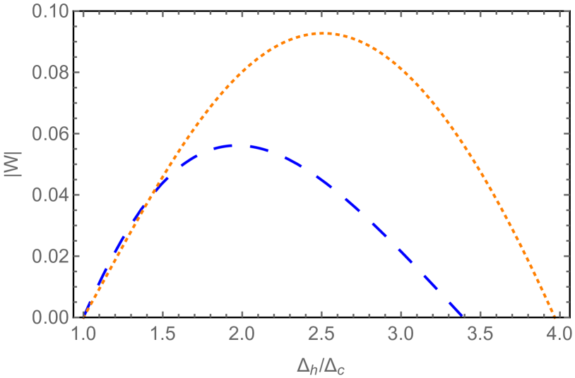
Figure 6: Adiabatic limit. Work output of the Otto cycle plotted as a function of the TLS tunneling at point $A$, $\Delta_{h}$, ignoring the decoupling cost for strong coupling (instantaneous decoupling case). Blue dashed curve: weak coupling; Orange dotted curve: strong coupling. Parameters (in units of $\Delta_{c}$): $\epsilon_{h}=\epsilon_{c}=1$, $\beta_{h}=1$, $\beta_{c}=2.5$, $\omega_{c}=2$, $\alpha=1$, and $n=30$ states are taken in the RC calculations.

We show a parametric plot of the work output against the efficiency of the engine for both strong and weak coupling in Fig. 5. The parameter which is varied along these curves is the bias, $\epsilon_{h}$, at point $A$. In the weak coupling regime, the efficiency increases monotonically with $\epsilon_{h}$ and saturates at the Carnot limit, $\eta_{C}=1-{T_{c}}/{T_{h}}$, at the point where the work output vanishes, $\mu_{c}/\mu_{h}=T_{c}/T_{h}$. The efficiency at maximum work output occurs prior to the Carnot bound being attained. The efficiency of the engine is inferior at strong coupling: work output is reduced in this regime and the energy absorbed from the hot reservoir is not reduced sufficiently to prevent a reduction in efficiency. We observe a qualitatively different behaviour compared with the weak coupling limit: the efficiency is maximised below the Carnot limit before turning over and falling to zero as the work output vanishes. This creates the loop structure of both the instantaneous decoupling and adiabatic decoupling curves. This structure is reminiscent of studies of heat engines containing some degree of internal frictional loss, for example in Ref. Alecce et al. (2015). The adiabatic decoupling protocol yields an improved efficiency, with some mitigation of the decoupling costs, and a loop which lies beyond the instantaneous decoupling case.

It is worth noting that for instantaneous decoupling in certain parameter regimes, the work output in the strong coupling case can beat the weak coupling limit when ignoring the decoupling cost. An example is shown in Fig. 6, where we vary $\Delta_{h}$ along the isentropic strokes rather than $\epsilon_{h}$. However, even in these situations the decoupling costs far outweigh such enhancements, and the cycle always displays a reduction in work output for the strong coupling calculations.

Finally, we consider how the engine performance scales with system-reservoir coupling strength $\alpha$ in Fig. 7. We observe that as the coupling strength is increased, the engine’s performance deteriorates in all but the weak coupling case, since there the magnitude of the interaction term is unimportant. Also, as expected, the weak coupling efficiency is recovered as $\alpha\rightarrow 0$. It is clear that the detrimental effect of the decoupling cost is more pronounced at higher couplings, and the adiabatic decoupling procedure becomes increasingly desirable, despite being unable to fully recover the weak coupling efficiency. In fact, for large enough couplings, it allows the cycle to perform as an engine even when the work output has vanished in the instantaneous decoupling case. It is also worth recognising that the sensitivity of the cycle performance to the system-reservoir decoupling procedure (instantaneous or adiabatic) is a feature inherent to the strong coupling regime, i.e. it is completely absent in the weak coupling treatment. Hence, it could be used (even at fixed $\alpha$) to signify the presence of strong coupling effects in experimental realisations of quantum heat engines.

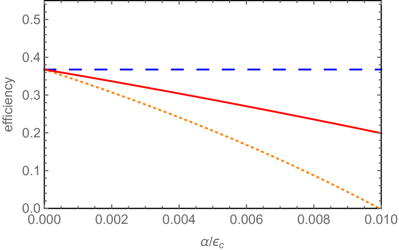
Figure 7: Adiabatic limit. Efficiency of the Otto engine plotted as a function of coupling strength $\alpha$. Blue dashed line: weak coupling; Orange dotted curve: strong coupling with instantaneous decoupling of the reservoirs; Red solid curve: strong coupling with adiabatic decoupling of the reservoirs. Parameters as in Fig. 3 with $\epsilon_{h}/\epsilon_{c}=2$.

III.2 Sudden isentropic strokes

We move now to the sudden limit of the Otto cycle, where the isentropes are carried out so quickly that the quantum state has no time to evolve along the stroke. The states at $C$ and $A$ thus read $\chi^{C}=\chi^{B^{\prime}}$ and $\chi^{A}=\chi^{D^{\prime}}$, which alters the respective energy expressions at these points. Working through the cycle (assuming instantaneous decoupling), we find that in the sudden limit the net work output reads

$$W= \textrm{tr}\left[H_{S}^{B}(\rho_{c}-\rho_{h})\right]+\textrm{tr}\left[H_{S}^{C}(\rho_{h}-\rho_{c})\right]$$

$$-\textrm{tr}[H_{I_{h}}\rho_{h}]-\textrm{tr}[H_{I_{c}}\rho_{c}],$$ (69)

while the energy absorbed from the hot reservoir becomes

$$Q^{A^{\prime}B}= \textrm{tr}\left[H_{S}^{B}(\rho_{h}-\rho_{c})\right]$$

$$+\textrm{tr}\left[H_{R_{h}}(\rho_{h}-\rho_{R_{h}})\right]+\textrm{tr}\left[H_{R_{c}}(\rho_{R_{c}}-\rho_{c})\right]$$

$$+\textrm{tr}[H_{I_{h}}\rho_{h}].$$ (70)

Both expressions may be evaluated within the RC formalism, as was the case in the adiabatic treatment.

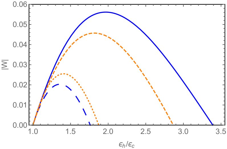
Figure 8: Comparing the adiabatic and sudden limits. Work output of the Otto cycle plotted as a function of the TLS bias at point $A$, $\epsilon_{h}$, ignoring the decoupling cost for strong coupling. Blue solid curve: weak coupling adiabatic; Orange (small) dashed curve: strong coupling adiabatic with instantaneous decoupling; Blue (large) dashed curve: weak coupling sudden; Orange dotted curve: strong coupling sudden. Parameters as in Fig. 3 though with $\alpha/\epsilon_{c}=0.1$.

It is well known that operating the cycle in the sudden limit introduces a process known as quantum friction Rezek and Kosloff (2006); Çakmak et al. (2016), which impacts negatively on the performance of the engine. This is apparent, for instance, in Fig. 8, where we note a large reduction in the weak coupling work output as compared to the adiabatic limit. Interestingly, we see that in this example the effect of quantum friction is less pronounced in the strong coupling regime, and indeed if it were not for the cost of decoupling (which outweighs the benefit), the strong coupling engine would outperform its weakly coupled counterpart. The impacts of the decoupling cost on the work output and energy conversion efficiency are shown in Fig. 9. In this figure, we see both the effect of quantum friction leading to a loop-like structure qualitatively similar to those seen in Fig. 5, and the effect of finite coupling reducing work output and efficiency such that the loops become smaller. We find that the scaling of engine performance with coupling strength is qualitatively similar to the adiabatic isentrope limit in Fig. 7.

IV Discussion

We have studied a quantum heat engine in the regime of strong coupling between the system and reservoirs, employing the RC formalism to account for the resulting generation of system-reservoir correlations. Considering the quantum Otto cycle, we have shown that the work cost incurred in decoupling the system and reservoirs impacts negatively on the engine, and have established that a variation of the cycle can help to improve its performance at strong coupling.

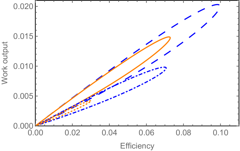
Figure 9: Sudden limit. Parametric plots of work output against efficiency in the sudden regime for a quantum Otto cycle plotted by varying the TLS bias at point $A$, $\epsilon_{h}$, for two different temperatures of the cold reservoir. Blue dashed curve: weak coupling and $\beta_{c}=2.5$; Orange solid curve: strong coupling and $\beta_{c}=2.5$; Blue dot-dashed curve: weak coupling $\beta_{c}=1.75$; Orange dotted curve: strong coupling $\beta_{c}=1.75$. Parameters (in units of $\epsilon_{c}$): $\Delta_{h}=\Delta_{c}=1$, $\beta_{h}=1$, $\omega_{c}=2$, $\alpha=0.001$, and $n=30$ states are taken in the RC calculations.

At the heart of our treatment lie the TLS-reservoir interactions, which we have modelled as being of spin-boson form. As such, we had to specify a certain spectral density, here chosen to be Ohmic. Extending the RC formalism of Refs. Iles-Smith et al. (2014, 2016) to other forms of spectral density is the subject of ongoing work, and should yield further understanding on the generality of our results. There are also alternative theoretical techniques, for example the polaron transformation Gelbwaser-Klimovsky and Aspuru-Guzik (2015); Nazir and McCutcheon (2016), that could be used to perform a similar and complementary analysis.

Several experimental realisations of nanoscale heat engines have been proposed Roßnagel et al. (2016); Abah et al. (2012); Jordan et al. (2013); Sothmann et al. (2015); Hofer and Sothmann (2015); Hofer et al. (2016). Although the protocols presented here are idealised in that they involve complete decoupling of the system from the reservoirs at various points during the engine cycle, it is certainly possible to control very precisely parameters such as the bias and tunnelling, for example, in experimental realisations of double well quantum dots in semiconductor nanowires Liu et al. (2015, 2014). An experimental realisation of a single-atom heat engine has recently been achieved Roßnagel et al. (2016), indicating that tuning the interaction strength as required for protocols such as those outlined here is possible. The theoretical description of nanoscale quantum engines which do not require decoupling from the reservoirs is given by continuously coupled models, recently reviewed in Ref. Kosloff and Levy (2014). The access afforded by the RC formalism to hitherto unexplored regimes are compelling reasons to apply the techniques discussed here to such models, as in Ref. Strasberg et al. (2016).

For the purposes of this work, we have considered an idealised version of the Otto cycle where full equilibration occurs along the isochores and the isentropic strokes are carried out either in the adiabatic or sudden limit. Extensions to finite time versions of the cycle could also be studied, in which case work output and efficiency become functions of the cycle time, and a power output may be defined. Considering such a cycle within the RC formalism would enable us to evaluate finite power situations at strong coupling, where full equilibration does not occur along the isochoric strokes. The question of whether strong system-reservoir couplings are also detrimental for the performance of finite time cycles is an important and interesting one, which merits further investigation.

Let us finally comment that the RC formalism has allowed us to consider explicitly the work costs involved in coupling and decoupling the system and the reservoirs around a heat engine cycle. These costs are typically ignored in the weak coupling limit where it is assumed that the interaction term in the Hamiltonian is small enough that the reservoirs remain in thermal equilibrium, and so linear interaction terms may be considered free. This assumption is frequently valid in classical thermodynamic systems, though at the quantum scale this need not necessarily be so. It may be argued that in considering such costs, we have had to specify a particular microscopic model of a heat engine and that, as a result, the emerging thermodynamics becomes model dependent. As such, one loses the appealing generality at the heart of the success of classical thermodynamics. We would argue in response that at strong coupling, whether on the quantum or classical scale, given that the Hamiltonian interaction terms become appreciable, a model specific description of thermodynamics may be inevitable. In which case, a formalism such as the RC method that allows for a physically intuitive treatment of these interactions holds great promise.

Acknowledgments—The authors wish to thank Philipp Strasberg and Neill Lambert for interesting discussions, comments, and for sharing their related manuscript on nonequilibrium thermodynamics in the strong coupling regime prior to publication. We also thank Obinna Abah, Zach Blunden-Codd, and Adam Stokes for discussions. DN is supported by the EPSRC. FM is supported by ERCG grant ODYCQUENT. AN is supported by The University of Manchester and the EPSRC.

*

Appendix A Adiabatic reservoir decoupling

In this Appendix we consider the possibility of mitigating some of the work cost associated with decoupling from the hot and cold reservoirs at points $B^{\prime}$ and $D^{\prime}$, respectively. If, at the end of the hot isochore, we consider decoupling the reservoir from the system adiabatically, the state at $B^{\prime}$ then differs from that at $B$ and reads

$$\chi^{B^{\prime}}=\rho_{S_{h}}\otimes\rho_{th_{h}}\otimes\rho_{th_{c}},$$ (71)

see Eqs. (31) - (33). Computing the cost of decoupling now yields

$$\langle H\rangle^{B^{\prime}}-\langle H\rangle^{B}= \textrm{tr}\left[H_{S}^{B}(\rho_{S_{h}}-\rho_{h})\right]+\textrm{tr}\left[H_{R_{h}}(\rho_{th_{h}}-\rho_{h})\right]$$

$$-\textrm{tr}\left[H_{I_{h}}\rho_{h}\right].$$ (72)

This cost remains zero in the standard weak coupling analysis. For strong coupling, however, it will involve both a work contribution and heat dissipation into the hot reservoir. We thus compute the change in free energy and equate this to the work associated with decoupling:

$$F_{B^{\prime}}-F_{B}= \langle H\rangle^{B^{\prime}}-\frac{1}{\beta_{h}}S(\chi^{B^{\prime}})-\left[\langle H\rangle^{B}-\frac{1}{\beta_{h}}S(\chi^{B})\right]$$

$$= \frac{1}{\beta_{h}}\ln\textrm{tr}\left[\exp\left(-\beta_{h}\left(H_{S}^{B}+H_{R_{h}}+H_{I_{h}}\right)\right)\right]$$

$$-\frac{1}{\beta_{h}}\ln Z_{S_{h}}-\frac{1}{\beta_{h}}\ln Z_{R_{h}},$$ (73)

where $S(\rho)=-\textrm{tr}\left[\rho\ln\rho\right]$ is the von Neumann entropy, $Z_{S_{h}}=\textrm{tr}\left[\exp\left(-\beta_{h}H_{S}^{B}\right)\right]$, and $Z_{R_{h}}=\textrm{tr}\left[\exp\left(-\beta_{h}H_{R_{h}}\right)\right]$. The heat dissipated into the bath during decoupling is then

$$Q_{BB^{\prime}} = \langle H\rangle^{B^{\prime}}-\langle H\rangle^{B}-\left[F_{B^{\prime}}-F_{B}\right],$$ (74)

and both the heat and work are calculated within the RC approach.

We also need to consider decoupling from the cold reservoir at point $D$. If the interaction is switched off adiabatically then the state at $D^{\prime}$ is given by

$$\chi^{D^{\prime}}=\rho_{S_{c}}\otimes\rho_{th_{h}}\otimes\rho_{th_{c}},$$ (75)

where

$$\rho_{S_{c}}=\frac{\exp\left(-\beta_{c}H_{S}^{C}\right)}{\textrm{tr}\left[\exp\left(-\beta_{c}H_{S}^{C}\right)\right]}.$$ (76)

The cost of decoupling may be evaluated in an analogous fashion to the hot reservoir case to yield

$$\langle H\rangle^{D^{\prime}}-\langle H\rangle^{D}= \textrm{tr}\left[H_{S}^{C}(\rho_{S_{c}}-\rho_{c})\right]+\textrm{tr}\left[H_{R_{c}}(\rho_{th_{c}}-\rho_{c})\right]$$

$$-\textrm{tr}\left[H_{I_{c}}\rho_{c}\right],$$ (77)

which may be partitioned into a work contribution and energy dissipated into the cold reservoir, just as was done for the hot reservoir.

For adiabatic decoupling, the expression for the net work output around a complete cycle then evaluates to

$$W = \left(\frac{\mu_{c}}{\mu_{h}}-1\right)\textrm{tr}\left[H_{S}^{B}\rho_{S_{h}}\right]+\left(\frac{\mu_{h}}{\mu_{c}}-1\right)\textrm{tr}\left[H_{S}^{C}\rho_{S_{c}}\right]$$ (78)

$$+\frac{1}{\beta_{h}}\ln\textrm{tr}\left[\exp\left(-\beta_{h}\left(H_{S}^{B}+H_{R_{h}}+H_{I_{h}}\right)\right)\right]$$

$$+\frac{1}{\beta_{c}}\ln\textrm{tr}\left[\exp\left(-\beta_{c}\left(H_{S}^{C}+H_{R_{c}}+H_{I_{c}}\right)\right)\right]$$

$$-\frac{1}{\beta_{h}}\ln Z_{S_{h}}-\frac{1}{\beta_{h}}\ln Z_{R_{h}}$$

$$-\frac{1}{\beta_{c}}\ln Z_{S_{c}}-\frac{1}{\beta_{c}}\ln Z_{R_{c}}.$$

To calculate the energy dissipated into the hot reservoir we need to consider both the contribution from the hot isochore and the subsequent decoupling, $Q=Q_{A^{\prime}B}+Q_{BB^{\prime}}$. We then find

$$Q= -\frac{\mu_{h}}{\mu_{c}}\textrm{tr}\left[H_{S}^{A}\rho_{S_{c}}\right]-\textrm{tr}\left[H_{S}^{B}\rho_{S_{h}}\right]$$

$$+\frac{1}{\beta_{h}}\ln Z_{S_{h}}+\frac{1}{\beta_{h}}\ln Z_{R_{h}}$$

$$-\ln\textrm{tr}\left[\exp\left(-\beta_{h}\left(H_{S}^{B}+H_{R_{h}}+H_{I_{h}}\right)\right)\right].$$ (79)

References

- Carnot (1824) S. Carnot, Réflexions sur la puissance motrice du feu: et sur les machines propres à développer cette puissance (Chez Bachelier, libraire, quai des Augustins, no. 55, A Paris, 1824).
- Blundell and Blundell (2010) S. Blundell and K. M. Blundell, Concepts in thermal physics, 2nd ed. (Oxford University Press, Oxford, 2010).
- Kosloff and Levy (2014) R. Kosloff and A. Levy, Annual Review of Physical Chemistry 65, 365 (2014).
- Gelbwaser-Klimovsky et al. (2015a) D. Gelbwaser-Klimovsky, W. Niedenzu, and G. Kurizki, Advances In Atomic, Molecular, and Optical Physics 64, 329 (2015a).
- Vinjanampathy and Anders (2016) S. Vinjanampathy and J. Anders, Contemporary Physics 57, 1 (2016).
- Kosloff (2013) R. Kosloff, Entropy 15, 2100 (2013).
- Skrzypczyk et al. (2014) P. Skrzypczyk, A. J. Short, and S. Popescu, Nat Commun 5 (2014).
- Scovil and Schulz-DuBois (1959) H. E. D. Scovil and E. O. Schulz-DuBois, Phys. Rev. Lett. 2, 262 (1959).
- Quan et al. (2007) H. T. Quan, Y.-X. Liu, C. P. Sun, and F. Nori, Phys. Rev. E 76, 031105 (2007).
- Kieu (2004) T. D. Kieu, Phys. Rev. Lett. 93, 140403 (2004).
- Scully et al. (2003) M. O. Scully, M. S. Zubairy, G. S. Agarwal, and H. Walther, Science 299, 862 (2003).
- Scully (2002) M. O. Scully, Phys. Rev. Lett. 88, 050602 (2002).
- Roßnagel et al. (2014) J. Roßnagel, O. Abah, F. Schmidt-Kaler, K. Singer, and E. Lutz, Phys. Rev. Lett. 112, 030602 (2014).
- Dillenschneider and Lutz (2009) R. Dillenschneider and E. Lutz, EPL (Europhysics Letters) 88, 50003 (2009).
- Abah and Lutz (2014) O. Abah and E. Lutz, EPL (Europhysics Letters) 106, 20001 (2014).
- Gelbwaser-Klimovsky et al. (2013) D. Gelbwaser-Klimovsky, R. Alicki, and G. Kurizki, Phys. Rev. E 87, 012140 (2013).
- Rezek and Kosloff (2006) Y. Rezek and R. Kosloff, New Journal of Physics 8, 83 (2006).
- Friedenberger and Lutz (2015) A. Friedenberger and E. Lutz, arXiv:1508.04128 (2015).
- Seifert (2016) U. Seifert, Phys. Rev. Lett. 116, 020601 (2016).
- Słowik et al. (2013) K. Słowik, R. Filter, J. Straubel, F. Lederer, and C. Rockstuhl, Phys. Rev. B 88, 195414 (2013).
- Hümmer et al. (2013) T. Hümmer, F. J. García-Vidal, L. Martín-Moreno, and D. Zueco, Phys. Rev. B 87, 115419 (2013).
- Le Hur (2012) K. Le Hur, Phys. Rev. B 85, 140506 (2012).
- Goldstein et al. (2013) M. Goldstein, M. H. Devoret, M. Houzet, and L. I. Glazman, Phys. Rev. Lett. 110, 017002 (2013).
- Peropadre et al. (2013) B. Peropadre, D. Zueco, D. Porras, and J. J. García-Ripoll, Phys. Rev. Lett. 111, 243602 (2013).
- Nazir and McCutcheon (2016) A. Nazir and D. P. S. McCutcheon, Journal of Physics: Condensed Matter 28, 103002 (2016).
- Wei et al. (2014) Y.-J. Wei, Y. He, Y.-M. He, C.-Y. Lu, J.-W. Pan, C. Schneider, M. Kamp, S. Höfling, D. P. S. McCutcheon, and A. Nazir, Phys. Rev. Lett. 113, 097401 (2014).
- Vogl and Weitz (2009) U. Vogl and M. Weitz, Nature 461, 70 (2009).
- Gelbwaser-Klimovsky et al. (2015b) D. Gelbwaser-Klimovsky, K. Szczygielski, U. Vogl, A. Saß, R. Alicki, G. Kurizki, and M. Weitz, Phys. Rev. A 91, 023431 (2015b).
- Note (1) We consider any situation in which the system-reservoir factorisation assumption fails to define the strong coupling regime.
- Ankerhold and Pekola (2014) J. Ankerhold and J. P. Pekola, Phys. Rev. B 90, 075421 (2014).
- Carrega et al. (2015) M. Carrega, P. Solinas, A. Braggio, M. Sassetti, and U. Weiss, New Journal of Physics 17, 045030 (2015).
- Esposito et al. (2015) M. Esposito, M. A. Ochoa, and M. Galperin, Phys. Rev. Lett. 114, 080602 (2015).
- Campisi et al. (2009) M. Campisi, P. Talkner, and P. Hänggi, Phys. Rev. Lett. 102, 210401 (2009).
- Campisi et al. (2011) M. Campisi, P. Hänggi, and P. Talkner, Rev. Mod. Phys. 83, 771 (2011).
- Hanggi and Talkner (2015) P. Hanggi and P. Talkner, Nat Phys 11, 108 (2015).
- Hörhammer and Büttner (2008) C. Hörhammer and H. Büttner, Journal of Statistical Physics 133, 1161 (2008).
- Esposito et al. (2010) M. Esposito, K. Lindenberg, and C. V. den Broeck, New Journal of Physics 12, 013013 (2010).
- Deffner and Lutz (2011) S. Deffner and E. Lutz, Phys. Rev. Lett. 107, 140404 (2011).
- Pucci et al. (2013) L. Pucci, M. Esposito, and L. Peliti, Journal of Statistical Mechanics: Theory and Experiment 2013, P04005 (2013).
- Gelbwaser-Klimovsky and Aspuru-Guzik (2015) D. Gelbwaser-Klimovsky and A. Aspuru-Guzik, The Journal of Physical Chemistry Letters 6, 3477 (2015).
- Strasberg et al. (2016) P. Strasberg, G. Schaller, N. Lambert, and T. Brandes, New Journal of Physics 18, 073007 (2016).
- Katz and Kosloff (2016) G. Katz and R. Kosloff, Entropy 18, 186 (2016).
- Gallego et al. (2014) R. Gallego, A. Riera, and J. Eisert, New Journal of Physics 16, 125009 (2014).
- Leggett et al. (1987) A. J. Leggett, S. Chakravarty, A. T. Dorsey, M. P. A. Fisher, A. Garg, and W. Zwerger, Rev. Mod. Phys. 59, 1 (1987).
- Weiss (2012) U. Weiss, Quantum Dissipative Systems (World Scientific, 2012).
- Nitzan (2013) A. Nitzan, Chemical Dynamics in Condensed Phases: Relaxation, Transfer, and Reactions in Condensed Molecular Systems (OUP Oxford, 2013).
- Breuer and Petruccione (2002) H.-P. Breuer and F. Petruccione, The theory of open quantum systems (Oxford University Press, Oxford, 2002).
- Schlosshauer (2007) M. A. Schlosshauer, Decoherence and the quantum-to-classical transition (Springer, Berlin, 2007).
- Iles-Smith et al. (2014) J. Iles-Smith, N. Lambert, and A. Nazir, Phys. Rev. A 90, 032114 (2014).
- Liu et al. (2015) Y.-Y. Liu, J. Stehlik, C. Eichler, M. J. Gullans, J. M. Taylor, and J. R. Petta, Science 347, 285 (2015).
- Liu et al. (2014) Y.-Y. Liu, K. D. Petersson, J. Stehlik, J. M. Taylor, and J. R. Petta, Phys. Rev. Lett. 113, 036801 (2014).
- Gilmore et al. (2005) J. Gilmore, and R. McKenzie, Journal of Physics: Condensed Matter 17, 1735 (2005).
- Gullans et al. (2015) M. J. Gullans, Y.-Y. Liu, J. Stehlik, J. R. Petta, and J. M. Taylor, Phys. Rev. Lett. 114, 196802 (2015).
- Shevchenko et al. (2010) S. Shevchenko, S. Ashhab, and F. Nori, Physics Reports 492, 1 (2010).
- Iles-Smith et al. (2016) J. Iles-Smith, A. G. Dijkstra, N. Lambert, and A. Nazir, The Journal of Chemical Physics 144, 044110 (2016).
- Note (2) The mapped Hamiltonian defined in Eq. (14) differs from that given in Eq. of Ref. Iles-Smith et al., 2014 in that it does not include an extra term that is quadratic in the RC creation and annihilation operators, and the couplings . As explained in Ref. Iles-Smith et al. (2014), there the term is added to cancel energy shifts that appear in the master equation governing the dynamics of the enlarged system. However, as we shall be concerned here with steady state solutions for the enlarged system, which are independent of the quadratic term, it has no bearing in our case, and we work directly with the mapped Hamiltonian as given in Eq. (14).
- Alecce et al. (2015) A. Alecce, F. Galve, N. Lo Gullo, L. Dell’Anna, F. Plastina, and R. Zambrini, New Journal of Physics 17, 075007 (2015).
- Çakmak et al. (2016) S. Çakmak, F.Altintas, and Ö. E. Müstecaplioğlu, Physica Scripta 91, 075101 (2016).
- Roßnagel et al. (2016) J. Roßnagel, S. T. Dawkins, K. N. Tolazzi, O. Abah, E. Lutz, F. Schmidt-Kaler, and K. Singer, Science 352, 325 (2016).
- Abah et al. (2012) O. Abah, J. Roßnagel, G. Jacob, S. Deffner, F. Schmidt-Kaler, K. Singer, and E. Lutz, Phys. Rev. Lett. 109, 203006 (2012).
- Jordan et al. (2013) A. N. Jordan, B. Sothmann, R. Sánchez, and M. Büttiker, Phys. Rev. B 87, 075312 (2013).
- Sothmann et al. (2015) B. Sothmann, R. Sánchez, and A. N. Jordan, Nanotechnology 26, 032001 (2015).
- Hofer and Sothmann (2015) P. P. Hofer and B. Sothmann, Phys. Rev. B 91, 195406 (2015).
- Hofer et al. (2016) P. P. Hofer, J.-R. Souquet, and A. A. Clerk, Phys. Rev. B 93, 041418 (2016).