A Cubic-Time 2-Approximation Algorithm for rSPR Distance

Abstract

Due to hybridization events in evolution, studying two different genes of a set of species may yield two related but different phylogenetic trees for the set of species. In this case, we want to measure the dissimilarity of the two trees. The rooted subtree prune and regraft (rSPR) distance of the two trees has been used for this purpose. The problem of computing the rSPR distance of two given trees has many applications but is NP-hard. The previously best approximation algorithm for rSPR distance achieves a ratio of 2 in polynomial time and its analysis is based on the duality theory of linear programming. In this paper, we present a cubic-time approximation algorithm for rSPR distance that achieves a ratio of $2$. Our algorithm is based on the notion of key and several structural lemmas; its analysis is purely combinatorial and explicitly uses a search tree for computing rSPR distance exactly.

Keywords: Phylogenetic tree, rSPR distance, approximation algorithm.

1 Introduction

When studying the evolutionary history of a set $X$ of existing species, one can obtain a phylogenetic tree $T_{1}$ with leaf set $X$ with high confidence by looking at a segment of sequences or a set of genes [12, 13]. When looking at another segment of sequences, a different phylogenetic tree $T_{2}$ with leaf set $X$ can be obtained with high confidence, too. In this case, we want to measure the dissimilarity of $T_{1}$ and $T_{2}$. The rooted subtree prune and regraft (rSPR) distance between $T_{1}$ and $T_{2}$ has been used for this purpose [11]. It can be defined as the minimum number of edges that should be deleted from each of $T_{1}$ and $T_{2}$ in order to transform them into essentially identical rooted forests $F_{1}$ and $F_{2}$. Roughly speaking, $F_{1}$ and $F_{2}$ are essentially identical if they become identical forests (called agreement forests of $T_{1}$ and $T_{2}$) after repeatedly contracting an edge $(p,c)$ in each of them such that $c$ is the unique child of $p$ (until no such edge exists).

The rSPR distance is an important metric that often helps us discover reticulation events. In particular, it provides a lower bound on the number of reticulation events [1, 2], and has been regularly used to model reticulate evolution [14, 15].

Unfortunately, it is NP-hard to compute the rSPR distance of two given phylogenetic trees [5, 11]. This has motivated researchers to design approximation algorithms for the problem [3, 4, 11, 16]. Hein et al. [11] were the first to come up with an approximation algorithm. They also introduced the important notion of maximum agreement forest (MAF) of two phylogenetic trees. Their algorithm was correctly analyzed by Bonet et al. [3]. Rodrigues et al. [16] modified Hein et al.’s algorithm so that it achieves an approximation ratio of 3 and runs in quadratic time. Whidden et al. [20] came up with a very simple approximation algorithm that runs in linear time and achieves an approximation ratio of 3. Although the ratio 3 is achieved by a very simple algorithm in [20], no polynomial-time approximation algorithm had been designed to achieve a better ratio than 3 before Shi et al. [10] presented a polynomial-time approximation algorithm that achieves a ratio of 2.5. Schalekamp et al. [17] presented a polynomial-time 2-approximation algorithm for the same problem. However, they use an LP-model of the problem and apply the duality theory of linear programming in the analysis of their algorithm. Hence, their analysis is not intuitively understandable. Moreover, they did not give an explicit upper bound on the running time of their algorithm. Unaware of Schalekamp et al.’s work [17], we [9] presented a quadratic-time $\frac{7}{3}$-approximation algorithm for the problem; the algorithm is relatively simpler and its analysis is purely combinatorial.

In certain real applications, the rSPR distance between two given phylogenetic trees is small enough to be computed exactly within reasonable amount of time. This has motivated researchers to take the rSPR distance as a parameter and design fixed-parameter algorithms for computing the rSPR distance of two given phylogenetic trees [5, 8, 18, 20, 19]. These algorithms are basically based on the branch-and-bound approach and use the output of an approximation algorithm (for rSPR distance) to decide if a branch of the search tree should be cut. Thus, better approximation algorithms for rSPR distance also lead to faster exact algorithms for rSPR distance. It is worth noting that approximation algorithms for rSPR distance can also be used to speed up the computation of hybridization number and the construction of minimum hybridization networks [6, 7].

In this paper, we improve our $\frac{7}{3}$-approximation algorithm in [9] to a new 2-approximation algorithm. Our algorithm proceeds in stages until the input trees $T_{1}$ and $T_{2}$ become identical forests. Roughly speaking, in each stage, our algorithm carefully chooses a dangling subforest $S$ of $T_{1}$ and uses $S$ to carefully choose and remove a set $B$ of edges from $T_{2}$. $B$ has a crucial property that the removal of the edges of $B$ decreases the rSPR distance of $T_{1}$ and $T_{2}$ by at least $\frac{1}{2}|B|$. Because of this property, our algorithm achieves a ratio of $2$. As in [9], the search of $S$ and $B$ in our algorithm is based on our original notion of key. However, unlike the algorithm in [9], the subforest $S$ in our new algorithm is not bounded from above by a constant. This difference is crucial, because the small bounded size of $S$ in [9] makes for a tedious case-analysis. Fortunately, we can prove a number of structural lemmas which enable us to construct $B$ systematically and hence avoid complicated case-analysis. Our analysis of the algorithm explicitly uses a search tree (for computing the rSPR distance of two given trees exactly) as a tool, in order to show that it achieves a ratio of 2. To our knowledge, we were the first to use a search tree explicitly for this purpose.

The remainder of this paper is organized as follows. Section 2 reviews the rSPR distance problem and presents our main theorems. Section 3 gives the basic definitions that will be used thereafter. Section 4 shows how to build a search tree for computing the rSPR distance exactly. Section 5 defines the important notion of key. Section 6 presents our algorithm for finding a good key or cut.

2 The rSPR Distance Problem and the Main Theorems

In this paper, a forest $F$ always means a rooted forest in which each vertex has at most two children. A vertex of $F$ is unifurcate (respectively, bifurcate) if its number of children in $F$ is 1 (respectively, 2). If a vertex $v$ of $F$ is not a root in $F$, then $e_{F}(v)$ denotes the edge entering $v$ in $F$; otherwise, $e_{F}(v)$ is undefined. For a set or sequence $U$ of vertices, $\ell_{F}(U)$ denotes the lowest common ancestor (LCA) of the vertices of $U$ in $F$ if the vertices of $U$ are in the same connected component of $F$, while $\ell_{F}(U)$ is undefined otherwise. When $\ell_{F}(U)$ is defined, we simply use $e_{F}(U)$ to denote $e_{F}(\ell_{F}(U))$.

$F$ is binary if it has no unifurcate vertex. Binarizing $F$ is the operation of modifying $F$ by repeatedly contracting an edge between a unifurcate vertex $p$ and its unique child $c$ into a single vertex $c$ until no vertex of $F$ is unifurcate. The binarization of $F$ is the forest obtained by binarizing $F$.

A phylogenetic forest is a binary forest $F$ whose leaves are distinctively labeled but non-leaves are unlabeled. Whenever we say that two phylogenetic forests are isomorphic, we always mean that the bijection also respects the leaf labeling. $F$ is a phylogeny if it is connected. Figure 1 shows two phylogenies $T$ and $F$. For convenience, we allow the empty phylogeny (i.e., the phylogeny without vertices at all) and denote it by $\bot$. For two phylogenetic forests $F_{1}$ and $F_{2}$ with the same set of leaf labels, we always view two leaves of $F_{1}$ and $F_{2}$ with the same label as the same vertex although they are in different forests.

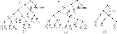
Figure 1: (1) A phylogeny $T$,  (2) another phylogeny $F$,  (3) $F\uparrow_{\{x_{1},\ldots,x_{4}\}}$.

Suppose that $F$ is a phylogenetic forest and $C$ is a set of edges in $F$. $F-C$ denotes the forest obtained from $F$ by deleting the edges in $C$. $F-C$ may not be phylogenetic, because it may have unlabeled leaves or unifurcate vertices. $F\ominus C$ denotes the phylogenetic forest obtained from $F-C$ by first removing all vertices without labeled descendants and then binarizing it. $C$ is a cut of $F$ if each connected component of $F-C$ has a labeled leaf. If in addition every leaf of $F-C$ is labeled, then $C$ is a canonical cut of $F$. For example, if $F$ is as in Figure 2(1), then the four dashed edges in $F$ form a canonical cut of $F$. It is known that if $C$ is a set of edges in $F$, then $F$ has a canonical cut $C^{\prime}$ such that $F\ominus C=F\ominus C^{\prime}$ [4].

Given a cut $\hat{C}$ of $F\ominus C$, we can extend $C$ to a cut $C^{\prime}$ of $F$ with $|C^{\prime}|=|C|+|\hat{C}|$ as follows. Clearly, $F-C$ is a subgraph of $F$. Let $F^{\prime}$ be the forest obtained from $F-C$ by removing all vertices without labeled descendants. Obviously, $F\ominus C$ can be transformed back into $F^{\prime}$ by replacing each edge $(u,v)$ of $F\ominus C$ with the path $P_{u,v}$ from $u$ to $v$ in $F$. Note that each vertex of $P_{u,v}$ other than $u$ and $v$ is unifurcate in $F^{\prime}$. For convenience, we refer to the edge of $P_{u,v}$ leaving $u$ as the edge of $F$ corresponding to the edge $(u,v)$ in $F\ominus C$. One can see that $C^{\prime}=C\cup\tilde{C}$ is a cut of $F$, where $\tilde{C}$ consists of the edges in $F$ corresponding to the edges in $\hat{C}$. Moreover, if both $C$ and $\hat{C}$ are canonical, then so is $C^{\prime}$.

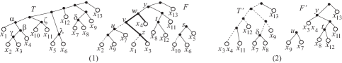
Figure 2: (1) A TF-pair $(T,F)$    (2) an induced sub-TF pair $(T^{\prime},F^{\prime})$ of $(T,F)$.

The rSPR Distance Problem: Given a pair $(T,F)$ of phylogenies with the same set of leaf-labels, find a cut $C_{T}$ in $T$ and a smallest cut $C_{F}$ in $F$ such that $T\ominus C_{T}$ and $F\ominus C_{F}$ are isomorphic.

For example, if $T$ and $F$ in Figure 1 are the input to the rSPR distance problem, then the dashed edges in $T$ and those in $F$ together form a possible output. In the above definition, we require that the size of $C_{F}$ be minimized; indeed, it is equivalent to require that the size of $C_{T}$ be minimized because the output $C_{T}$ and $C_{F}$ have the same size.

To solve the rSPR distance problem, it is more convenient to relax the problem by only requiring that $T$ be a phylogenetic tree (i.e., a connected phylogenetic forest) and $F$ be a phylogenetic forest. Hereafter, we assume that the problem has been relaxed in this way. Then, we refer to each input $(T,F)$ to the problem as a tree-forest (TF) pair. The size of the output $C_{F}$ is the rSPR distance of $T$ and $F$, and is denoted by $d(T,F)$. In the sequel, we assume that a TF-pair $(T,F)$ always satisfies that no leaf of $F$ is a root of $F$. This assumption does not lose generality, because we can remove $x$ from both $T$ and $F$ without changing $d(T,F)$ if $x$ is both a leaf and a root of $F$. By this assumption, $e_{F}(x)$ is defined for all leaves $x$ in $F$. We also assume that no two leaves $x$ and $y$ are siblings in both $T$ and $F$. This assumption does not lose generality, because we can contract the subtree of $T$ (respectively, $F$) rooted at the parent of $x$ and $y$ into a single leaf (whose label is, say the concatenation of those of $x$ and $y$) without changing $d(T,F)$.

It is worth pointing out that to compute $d(T,F)$, it is required in the literature that we preprocess each of $T$ and $F$ by first adding a new root and a dummy leaf and further making the old root and the dummy be the children of the new root. However, the common dummy in the modified $T$ and $F$ can be viewed as an ordinary labeled leaf and hence we do not have to explicitly mention the dummy when describing an algorithm.

To compute $d(T,F)$ for a given TF-pair $(T,F)$, it is unnecessary to compute both a cut $C_{T}$ in $T$ and a cut $C_{F}$ in $F$. Indeed, it suffices to compute only $C_{F}$, because a cut in $F$ forces a cut in $T$. To make this clear, we obtain a cut $C_{T}$ of $T$ from a (possibly empty) cut $C_{F}$ of $F$ as follows.

1. Initially, $C_{T}=\emptyset$.

2. While $T\ominus C_{T}$ has a non-root $\alpha$ such that the subtree of $T\ominus C_{T}$ rooted at $\alpha$ is isomorphic to a connected component of $F\ominus C_{F}$, add to $C_{T}$ the edge of $T$ corresponding to $(\beta,\alpha)$, where $\beta$ is the parent of $\alpha$ in $T\ominus C_{T}$.

We refer to $C_{T}$ obtained from $C_{F}$ as above as the cut of $T$ forced by $C_{F}$. For convenience, we say that a vertex $\alpha$ of $T\ominus C_{T}$ and a vertex $v$ of $F\ominus C_{F}$ agree if the subtree of $T\ominus C_{T}$ rooted at $\alpha$ is isomorphic to the subtree of $F\ominus C_{F}$ rooted at $v$. For example, if $C_{F}$ consists of the four dashed edges in Figure 2(1), then $C_{T}=\{e_{F}(x_{1}),e_{F}(x_{2}),e_{F}(x_{10}),e_{F}(\lambda)\}$, $\beta$ in $T\ominus C_{T}$ and $w$ in $F\ominus C_{F}$ agree, and so do $\lambda$ in $T\ominus C_{T}$ and $s$ in $F\ominus C_{F}$. We further define the sub-TF pair of $(T,F)$ induced by $C_{F}$ to be the TF pair $(T^{\prime},F^{\prime})$ obtained as follows.

1. Initially, $F^{\prime}=F\ominus C_{F}$ and $T^{\prime}=T\ominus C_{T}$, where $C_{T}$ is the cut of $T$ forced by $C_{F}$.

2. For each connected component $K$ of $F^{\prime}$ isomorphic to a connected component $H$ of $T^{\prime}$, delete $K$ and $H$ from $F^{\prime}$ and $T^{\prime}$, respectively.

3. Find the set $A$ of pairs $(\alpha,v)$ such that $\alpha$ and $v$ are non-leaves in $T^{\prime}$ and $F^{\prime}$ respectively and they agree but their parents do not.

4. For each $(\alpha,v)\in A$ (in any order), modify $T^{\prime}$ (respectively, $F^{\prime}$) by contracting the subtree rooted at $\alpha$ (respectively, $v$) into a single leaf $\tilde{\alpha}$ (respectively, $\tilde{v}$) and further assigning the same new label to $\tilde{\alpha}$ and $\tilde{v}$.

For example, if $C_{F}$ consists of the four dashed edges in Figure 2(1), then the sub-TF pair induced by $C_{F}$ is as in Figure 2(2). We can view $T^{\prime}$ (respectively, $F^{\prime}$) as a subgraph of $T\ominus C_{T}$ (respectively, $F\ominus C_{F}$), by viewing $\tilde{\alpha}$ (respectively, $\tilde{v}$) as $\alpha$ (respectively, $v$) for each $(\alpha,v)\in A$.

If $(T^{\prime},F^{\prime})=(\bot,\bot)$, then $C_{F}$ is an agreement cut of $(T,F)$ and $F\ominus C_{F}$ is an agreement forest of $(T,F)$. If in addition, $C_{F}$ is canonical, then $C_{F}$ is a canonical agreement cut of $(T,F)$. The smallest size of an agreement cut of $(T,F)$ is actually $d(T,F)$.

To compute an approximation of $d(T,F)$, our idea is to look at a local structure of $T$ and $F$ and find a cut within the structure. A cut $C$ of $F$ is good (respectively, fair) for $(T,F)$ if $d(T^{\prime},F^{\prime})\leq d(T,F)-\frac{1}{2}|C|$ (respectively, $d(T^{\prime},F^{\prime})\leq d(T,F)-\frac{1}{2}(|C|-1)$), where $(T^{\prime},F^{\prime})$ is the sub-TF pair of $(T,F)$ induced by $C$. It is trivial to find a fair cut $C$ for $(T,F)$ with $|C|=3$ [20]. In contrast, Theorem 2.1 is hard to prove and the next sections are devoted to its proof.

Theorem 2.1

Given a TF-pair $(T,F)$, we can find a good cut for $(T,F)$ in quadratic time.

Theorem 2.2

Given a TF-pair $(T,F)$, we can compute an agreement cut $C_{F}$ of $(T,F)$ with $|C_{F}|\leq 2d(T,F)$ in cubic time.

Proof. Given a TF-pair $(T,F)$, we first compute a good cut $C$ for $(T,F)$ and then construct the sub-TF pair $(T^{\prime},F^{\prime})$ of $(T,F)$ induced by $C$. If $(T^{\prime},F^{\prime})=(\bot,\bot)$, then we return $C$; otherwise, we recursively compute an agreement cut $C^{\prime}$ of $(T^{\prime},F^{\prime})$, and then return $C\cup C^{\prime\prime}$, where $C^{\prime\prime}$ consists of the edges in $F$ corresponding to those in $C^{\prime}$.

The correctness and time complexity of the above algorithm are clear. We next prove that the algorithm returns an agreement cut $C_{F}$ of $(T,F)$ with $|C_{F}|\leq 2d(T,F)$ by induction on the recursion depth of the algorithm. If the algorithm makes no recursive call, it is clear that the algorithm outputs an agreement cut $C$ of $(T,F)$ with $|C|\leq 2d(T,F)$. So, assume that the algorithm makes a recursive call. Then, $|C^{\prime}|\leq 2d(T^{\prime},F^{\prime})$ by the inductive hypothesis. Now, since $d(T^{\prime},F^{\prime})\leq d(T,F)-\frac{1}{2}|C|$, $|C\cup C^{\prime\prime}|=|C|+|C^{\prime}|\leq 2(d(T,F)-d(T^{\prime},F^{\prime}))+2d(T^{\prime},F^{\prime})=2d(T,F)$. $\Box$

3 Basic Definitions and Notations

Throughout this section, let $F$ be a phylogenetic forest. We view each vertex $v$ of $F$ as an ancestor and descendant of itself. Two vertices $u$ and $v$ of $F$ are comparable if $\ell_{F}(u,v)\in\{u,v\}$, while they are incomparable otherwise. For brevity, we refer to a connected component of $F$ simply as a component of $F$. We use $L(F)$ to denote the set of leaves in $F$, and use $|F|$ to denote the number of components in $F$. A dangling subtree of $F$ is the subtree rooted at a vertex of $F$.

Let $u_{1}$ and $u_{2}$ be two vertices in the same component of $F$. If $u_{1}$ and $u_{2}$ have the same parent in $F$, then they are siblings in $F$. We use $u_{1}\sim_{F}u_{2}$ to denote the path between $u_{1}$ and $u_{2}$ in $F$. Note that $u_{1}\sim_{F}u_{2}$ is not a directed path if $u_{1}$ and $u_{2}$ are incomparable in $F$. For convenience, we still view each edge of $u_{1}\sim_{F}u_{2}$ as a directed edge (whose direction is the same as in $F$) although $u_{1}\sim_{F}u_{2}$ itself may not be a directed path. Each vertex of $u_{1}\sim_{F}u_{2}$ other than $u_{1}$ and $u_{2}$ is an inner vertex of $u_{1}\sim_{F}u_{2}$. $D_{F}(u_{1},u_{2})$ denotes the set of edges $(p,c)$ in $F$ such that $p$ is an inner vertex of $u_{1}\sim_{F}u_{2}$ but $c$ does not appear in $u_{1}\sim_{F}u_{2}$. Moreover, if $u_{1}$ and $u_{2}$ are incomparable in $F$, then $D_{F}^{+}(u_{1},u_{2})$ denotes the set consisting of the edges in $D_{F}(u_{1},u_{2})$ and all defined $e_{F}(v)$ such that $v$ is a vertex of $u_{1}\sim_{F}u_{2}$ but $e_{F}(v)\neq e_{F}(u_{i})$ for each $i\in\{1,2\}$ with $u_{i}\in L(F)$; otherwise $D_{F}^{+}(u_{1},u_{2})=\emptyset$. For convenience, if $w_{1}$ and $w_{2}$ are two vertices in different components in $F$, we define $D_{F}(w_{1},w_{2})=\emptyset$ and $D_{F}^{+}(w_{1},w_{2})=\emptyset$. For example, in Figure 1(2), $D_{F}(x_{1},x_{9})=\{e_{F}(x_{7}),e_{F}(u),e_{F}(v),e_{F}(x_{3})\}$, while in Figure 2(2), $D_{T^{\prime}}^{+}(\delta,x_{11})$ consists of the eight dashed edges.

Let $X$ be a subset of $L(F)$, and $v$ be a vertex of $F$. A descendant $x$ of $v$ in $F$ is an $X$-descendant of $v$ if $x\in X$. $X^{F}(v)$ denotes the set of $X$-descendants of $v$ in $F$. If $X^{F}(v)\neq\emptyset$, then $v$ is $X$-inclusive; otherwise, $v$ is $X$-exclusive. If $v$ is a non-leaf and both children of $v$ are $X$-inclusive, $v$ is $X$-bifurcate. An edge of $F$ is $X$-inclusive (respectively, $X$-exclusive) if its head is $X$-inclusive (respectively, $X$-exclusive). For an $X$-bifurcate $v$ in $F$, an $X$-child of $v$ in $F$ is a descendant $u$ of $v$ in $F$ such that each edge in $D_{F}(v,u)$ is $X$-exclusive and either $u\in X$ or $u$ is $X$-bifurcate; we also call $v$ the $X$-parent of $u$ in $F$; note that $v$ has exactly two $X$-children in $F$ and we call them $X$-siblings. In particular, when $X=L(F)$, $X$-parent, $X$-children, and $X$-siblings become parent, children, and siblings, respectively. For example, if $F$ is as in Figure 2(1) and $X=\{x_{1},\ldots,x_{4}\}$, then $v$ is $X$-bifurcate and its $X$-children are $x_{2}$ and $z$. $F\uparrow_{X}$ denotes the phylogenetic forest obtained from $F$ by removing all $X$-exclusive vertices and all vertices without $X$-bifurcate ancestors. See Figure 1 for an example.

4 Search Trees

A simple way to compute $d(T,F)$ for a TF-pair $(T,F)$ is to build a search tree $\Gamma$ (whose edges each are associated with a set of edges in $F$) recursively as follows. If $(T,F)=(\bot,\bot)$, then $\Gamma$ has only one node and we are done. So, assume that $(T,F)\neq(\bot,\bot)$. We first construct the root $\rho$ of $\Gamma$. To construct the subtrees of $\Gamma$ rooted at the children of $\rho$, we choose a pair $(x_{1},x_{2})$ of sibling leaves in $T$ and distinguish two cases as follows:

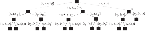
Figure 3: A search tree for the TF-pair $(T^{\prime},F^{\prime})$ in Figure 2(2).

Case 1: $x_{1}$ and $x_{2}$ fall into the same component of $F$. In this case, let $C_{1}=\{e_{F}(x_{1})\}$, $C_{2}=\{e_{F}(x_{2})\}$, and $C_{3}=D_{F}(x_{1},x_{2})$. For each $i\in\{1,\ldots,3\}$, we recursively construct a search tree $\Gamma_{i}$ for the sub-TF pair induced by $C_{i}$, make the root $\rho_{i}$ of $\Gamma_{i}$ be the $i$-th child of $\rho$ by adding the edge $(\rho,\rho_{i})$, associate $C_{i}$ with the edge $(\rho,\rho_{i})$, and modify the set $C$ associated with each edge in $\Gamma_{i}$ by replacing each $e\in C$ with the edge of $F$ corresponding to $e$.

Case 2: $x_{1}$ and $x_{2}$ fall into different components of $F$. In this case, $D_{F}(x_{1},x_{2})$ is undefined; we construct $\Gamma$ as in Case 1 by ignoring $C_{3}$, i.e., we do not construct the third child and its descendants.

Note that the children of each node in $\Gamma$ are ordered. This finishes the construction of $\Gamma$. See Figure 3 for an example.

A path in $\Gamma$ is a root-path if it starts at the root of $\Gamma$. For a root-path $P$ in $\Gamma$, we use $C(P)$ to denote the union of the sets associated with the edges in $P$. Clearly, $C(P)$ is a canonical cut of $F$. In particular, $C(P)$ is a canonical agreement cut of $(T,F)$ if $P$ ends at a leaf node of $\Gamma$. For a node $\varpi$ in $\Gamma$, we use $C(\varpi)$ to denote $C(P_{\varpi})$, where $P_{\varpi}$ is the path from the root to $\varpi$ in $\Gamma$.

Let $\varpi$ be a non-leaf node in $\Gamma$, $C_{T}$ be the cut of $T$ forced by $C(\varpi)$, $(T^{\prime},F^{\prime})$ be the sub-TF pair of $(T,F)$ induced by $C(\varpi)$, and $(\alpha_{1},\alpha_{2})$ be the pair of sibling leaves in $T^{\prime}$ selected to construct the children of $\varpi$ in $\Gamma$. The cherry picked at $\varpi$ is $(Y_{1},Y_{2})$, where for each $i\in\{1,2\}$, $Y_{i}$ is the set of leaf descendants of $\alpha_{i}$ in $T\ominus C_{T}$. For example, if $(T,F)$ is the same as $(T^{\prime},F^{\prime})$ in Figure 2(2), then the cherry picked at $\varpi$ is $(\{x_{3}x_{4},x_{11}\},\{x_{12}\})$.

A root-path $P$ in $\Gamma$ picks a cherry $(Y_{1},Y_{2})$ if $P$ contains a node $\varpi$ at which $P$ does not end and the cherry picked is $(Y_{1},Y_{2})$. If in addition, $P$ contains the $k$-th child of $\varpi$, then $P$ picks $(Y_{1},Y_{2})$ in the $k$-th way. Moreover, $P$ isolates $Y_{k}$ if $k\in\{1,2\}$, while $P$ creates $Y_{1}\cup Y_{2}$ if $k=3$.

$(T,F)$ may have multiple search trees (depending on the order of cherries picked by root-paths in a search tree). Nonetheless, it is widely known that for each search tree $\Gamma$ of $(T,F)$, $d(T,F)=\min_{\varpi}|C(\varpi)|$, where $\varpi$ ranges over all leaf nodes of $\Gamma$ [19]. Basically, this is true because a search tree represents an exhaustive search of a smallest agreement cut of $(T,F)$.

Let $Z$ be a set of leaves in $T$ such that each component of $T\uparrow_{Z}$ is a dangling subtree of $T$. A search tree $\Gamma$ of $(T,F)$ respects $Z$, if $P$ can be cut into two portions $P_{1}$ and $P_{2}$ such that $P_{1}$ starts at the root of $\Gamma$ and always picks a cherry $(Z_{1},Z_{2})$ with $Z_{1}\cup Z_{2}\subseteq Z$ while $P_{2}$ never picks such a cherry. Since each component of $T\uparrow_{Z}$ is a dangling subtree of $T$, at least one search tree of $(T,F)$ respects $Z$. For each search tree $\Gamma$ of $(T,F)$ respecting $Z$, the tree obtained from $\Gamma$ by deleting all nodes at which the cherries $(Z_{1},Z_{2})$ picked satisfy $Z_{1}\cup Z_{2}\not\subseteq Z$ is called a $Z$-search tree of $(T,F)$. For example, the dashed lines in Figure 3 form a $\{x_{3}x_{4},x_{11},x_{12}\}$-search tree for the TF-pair $(T^{\prime},F^{\prime})$ in Figure 2(2).

Let $\Gamma_{Z}$ be a $Z$-search tree of $(T,F)$. A root-leaf path in $\Gamma_{Z}$ is a root-path $P$ in $\Gamma_{Z}$ ending at a leaf node of $\Gamma_{Z}$. Since each $Z$-search tree $\Gamma_{Z}$ of $(T,F)$ can be extended to a search tree of $(T,F)$, the following hold:

• For each root-leaf path $P$ in $\Gamma_{Z}$, $C(P)$ is a canonical cut of $F$ and can be extended to a canonical agreement cut of $(T,F)$.

• $\Gamma_{Z}$ has at least one root-leaf path $P$ such that $C(P)$ can be extended to a smallest canonical agreement cut of $(T,F)$.

5 Keys and Lower Bounds

Throughout this section, let $(T,F)$ be a TF pair. Instead of cuts, we consider a more useful notion of key. Intuitively speaking, a key contains not only a cut $B$ within a local structure of $F$ but also possibly two leaves in $F\ominus B$ to be merged into a single leaf. Formally, a key of $(T,F)$ is a triple $\kappa=(X,B,R)$ satisfying the following conditions:

1. $X$ is a set of leaves in $T$ such that each component of $T\uparrow_{X}$ is a dangling subtree of $T$.

2. $B\subseteq E_{X}$ is a cut of $F$, where $E_{X}$ is the set of edges in $F$ whose tails or heads appear in $F\uparrow_{X}$. Moreover, either $\{e_{F}(x)~{}|~{}x\in X\}\subseteq B$ or $|\{e_{F}(x)~{}|~{}x\in X\}\setminus B|=2$.

3. If $\{e_{F}(x)~{}|~{}x\in X\}\subseteq B$, then $R=\emptyset$; otherwise, for the two vertices $x_{1}$ and $x_{2}$ in $X$ with $\{e_{F}(x_{1}),e_{F}(x_{2})\}=\{e_{F}(x)~{}|~{}x\in X\}\setminus B$, we have that $x_{1}$ and $x_{2}$ are siblings in $F\ominus B$, $R$ is the edge set of $x_{1}\sim_{F}x_{2}$, and $B\cap R=\emptyset$. (Comment: By Condition 1, $x_{1}$ and $x_{2}$ are siblings in $T\ominus\{e_{T}(x)~{}|~{}x\in X\setminus\{x_{1},x_{2}\}\}$ as well. So, when we compute the sub-TF pair of $(T,F)$ induced by $B$, $x_{1}\sim_{F}x_{2}$ will be contracted into a single leaf and so will $x_{1}\sim_{T}x_{2}$.)

For example, if $(T,F)$ is as in Figure 2(1), then $\kappa_{e}=(X,B,R)$ is a key of $(T,F)$, where $X=\{x_{2},x_{3},x_{4}\}$, $B=\{e_{F}(x_{1}),e_{F}(x_{2}),e_{F}(u)\}$, and $R$ is the edge set of $x_{3}\sim_{F}x_{4}$.

If $R=\emptyset$, then $\kappa$ is normal and we simply write $\kappa=(X,B)$ instead of $\kappa=(X,B,R)$; otherwise, it is abnormal. In essence, only normal keys were considered in [10].

Let $\kappa=(X,B,R)$ be a key of $(T,F)$. The size of $\kappa$ is $|B|$ and is also denoted by $|\kappa|$. The sub-TF pair of $(T,F)$ induced by $\kappa$ is the sub-TF pair $(T^{\prime},F^{\prime})$ of $(T,F)$ induced by $B$. Let $Y$ be a subset of $L(T)$ such that $X\subseteq Y$ and each component in $T\uparrow_{Y}$ is a dangling subtree of $T$. Further let $P$ be a root-leaf path in a $Y$-search tree of $(T,F)$. A component $K$ in $F-((C(P)\setminus R)\cup B)$ is free if $K$ contains no labeled leaf. We use $f_{c}(\kappa,P)$ to denote the set of free components in $F-((C(P)\setminus R)\cup B)$, and use $f_{e}(\kappa,P)$ to denote $C(P)\cap(B\cup R)$. The lower bound achieved by $\kappa$ $w.r.t.$ $P$ is $b(\kappa,P)=|f_{e}(\kappa,P)|+|f_{c}(\kappa,P)|$.

The lower bound achieved by $\kappa$ via $Y$ is $b_{Y}(\kappa)=\displaystyle\max_{\Gamma}\min_{P}b(\kappa,P)$, where $\Gamma$ ranges over all $Y$-search trees of $(T,F)$ and $P$ ranges over all root-leaf paths in $\Gamma$. If $\Gamma$ is a $Y$-search tree of $(T,F)$ with $b_{Y}(\kappa)=\min_{P}b(\kappa,P)$ where $P$ ranges all root-leaf paths in $\Gamma$, then $\Gamma$ is called a $Y$-search tree of $(T,F)$ witnessing $b_{Y}(\kappa)$. When $Y=X$, we write $b(\kappa)$ instead of $b_{X}(\kappa)$. The next two lemmas may help the reader understand the definitions (especially for abnormal keys) and will also be useful later.

Lemma 5.1

Suppose that $T$ has a pair $(x_{1},x_{2})$ of sibling leaves such that $\ell_{F}(x_{1},x_{2})$ exists and $1\leq|D_{F}(x_{1},x_{2})|\leq 2$. Then, $(T,F)$ has an abnormal key $\kappa$ with $|\kappa|\leq 2$ and $b(\kappa)\geq 1$.

Proof. Let $\kappa=(X,B,R)$, where $X=\{x_{1},x_{2}\}$, $B=D_{F}(x_{1},x_{2})$, and $R$ is the edge set of $x_{1}\sim_{F}x_{2}$. A root-leaf path $P$ in the unique $X$-search tree of $(T,F)$ either creates $X$ or isolates one of $\{x_{1}\}$ and $\{x_{2}\}$. In the former case, $B\subseteq C(P)$ and in turn $|C(P)\cap B|\geq 1$. In the latter case, $e_{F}(x_{1})\in C(P)$ or $e_{F}(x_{2})\in C(P)$, and hence $|C(P)\cap R|\geq 1$. $\Box$

Lemma 5.2

Suppose that $T$ has two pairs $(x_{1},x_{2})$ and $(x_{3},x_{4})$ of sibling leaves such that $x_{1}$ and $x_{3}$ are siblings in $F$ and so are $x_{2}$ and $x_{4}$. Then, $(T,F)$ has a normal key $\hat{\kappa}=(\{x_{1},\ldots,x_{4}\},\hat{B})$ with $|\hat{\kappa}|\leq 2b(\hat{\kappa})$.

Proof. Let $\hat{X}=\{x_{1},\ldots,x_{4}\}$ and $\hat{B}=\{e_{F}(x_{1}),\ldots,e_{F}(x_{4})\}$. Consider an $X$-search tree $\Gamma$ of $(T,F)$ in which each root-leaf path $P$ first picks the cherry $(\{x_{1}\},\{x_{2}\})$ and then picks the cherry $(\{x_{3}\},\{x_{4}\})$. If for some $i\in\{1,3\}$, $P$ creates $\{x_{i},x_{i+1}\}$, then $C(P)$ contains both $e_{F}(x_{4-i})$ and $e_{F}(x_{5-i})$. Otherwise, $C(P)$ contains $e_{F}(x_{i})$ and $e_{F}(x_{j})$ for some $i\in\{1,2\}$ and $j\in\{3,4\}$. So, in any case, $|C(P)\cap B|=2$. $\Box$

For the next three lemmas, let $\kappa=(X,B,R)$ be a key of $(T,F)$. The lemmas show why we can call $b_{L(T)}(\kappa)$ a lower bound. The next lemma is obvious.

Lemma 5.3

Let $P$ be a root-leaf path in an $X$-search tree of $(T,F)$, and $H$ be a component in $f_{c}(\kappa,P)$. Then, there is no $e\in R$ such that some endpoint of $e$ is in $H$. Moreover, either the root $r_{H}$ of $H$ is a root in $F$, or $(C(P)\setminus R)\cup B$ contains $e_{F}(r_{H})$.

Lemma 5.4

Let $Y$ be a subset of $L(T)$ such that $X\subseteq Y$ and each component in $T\uparrow_{Y}$ is a dangling subtree of $T$. Then, $b_{Y}(\kappa)\leq b_{L(T)}(\kappa)$.

Proof. Let $\Gamma_{Y}$ be a $Y$-search tree of $(T,F)$ witnessing $b_{Y}(\kappa)$. As aforementioned, we can extend $\Gamma_{Y}$ to a search tree $\Gamma$ of $(T,F)$. In other words, each root-leaf path $P_{Y}$ in $\Gamma_{Y}$ is the first portion of a root-leaf path $P$ in $\Gamma$. Since $C(P_{Y})\subseteq C(P)$, $C(P_{Y})\cap(B\cup R)\subseteq C(P)\cap(B\cup R)$, and $|f_{c}(\kappa,P_{Y})|\leq|f_{c}(\kappa,P)|$. In summary, $b(\kappa,P_{Y})\leq b(\kappa,P)$. $\Box$

The next lemma shows why $b(\kappa)$ is a lower bound on $d(T,F)-d(T^{\prime},F^{\prime})$.

Lemma 5.5

Let $P$ be a root-leaf path in a search tree of $(T,F)$ such that $C(P)$ is a smallest canonical agreement cut of $(T,F)$. Then, $d(T,F)-d(T^{\prime},F^{\prime})\geq b(\kappa,P)$, where $(T^{\prime},F^{\prime})$ is the sub-TF pair of $(T,F)$ induced by $\kappa$. Consequently, $d(T,F)-d(T^{\prime},F^{\prime})\geq b_{L(T)}(\kappa)\geq b(\kappa)$.

Proof. Let $M=C(P)\setminus R$. Obviously, $|M|=|C(P)|-|C(P)\cap R|=d(T,F)-|C(P)\cap R|$ and $F-M$ has $|F|+d(T,F)-|C(P)\cap R|$ components. Since $C(P)$ is a canonical cut of $F$, every component in $F-C(P)$ has a labeled leaf. So, $F\ominus M$ has the same number of components as $F-M$. Moreover, $|B\setminus M|=|B|-|C(P)\cap B|$ and in turn $F-(M\cup B)$ has exactly $|F\ominus M|+|B|-|C(P)\cap B|$ components among which $f_{c}(\kappa,P)$ have no labeled leaves. Hence, $|F\ominus(M\cup B)|\leq\left(d(T,F)+|F|-|C(P)\cap R|\right)+\left(|B|-|C(P)\cap B|-|f_{c}(\kappa,P)|\right)=|F|+|B|+d(T,F)-b(\kappa,P)$.

Since $F\ominus C(P)$ is an agreement forest of $(T,F)$, $F\ominus(C(P)\cup B)$ is clearly an agreement forest of $(T,F\ominus B)$. So, by Condition 3 in the definition of keys, $F\ominus(M\cup B)$ is also an agreement forest of $(T,F\ominus B)$. Now, since $|F\ominus B|=|F|+|B|$, $(T,F\ominus B)$ has an agreement cut of size at most $d(T,F)-b(\kappa,P)$. On the other hand, a smallest agreement cut of $(T,F\ominus B)$ is of size $d(T^{\prime},F^{\prime})$. Hence, $d(T,F)-d(T^{\prime},F^{\prime})\geq b(\kappa,P)$. Therefore, $d(T,F)-d(T^{\prime},F^{\prime})\geq b_{L(T)}(\kappa)$, and in turn $d(T,F)-d(T^{\prime},F^{\prime})\geq b(\kappa)$ by Lemma 5.4. $\Box$

A key $\kappa$ of $(T,F)$ is good if $|\kappa|\leq 2b_{L(T)}(\kappa)$, while $\kappa$ is fair if $|\kappa|\leq 2b_{L(T)}(\kappa)+1$). Obviously, for each leaf $x$ of $T$, $(\{x\},\{e_{F}(x)\})$ is a fair key of $(T,F)$. If $\kappa=(X,B,R)$ is a good key of $(T,F)$, then by Lemma 5.5, $B$ is a good cut of $F$. So, in order to find a good cut of $F$, it suffices to find a good key of $(T,F)$.

The next three lemmas can often help us estimate $f_{e}(\kappa,P)$ and $f_{c}(\kappa,P)$. For the three lemmas, let $\kappa=(X,B)$ be a normal key of $(T,F)$, and $P$ be a root-leaf path in an $X$-search tree $\Gamma_{X}$ of $(T,F)$ witnessing $b(\kappa)$.

Lemma 5.6

Suppose that $(\varpi_{1},\varpi_{2})$ is an edge in $P$ such that some edge $e_{F}(v)\in C(\varpi_{2})\setminus C(\varpi_{1})$ satisfies that the set $Y$ of labeled-leaf descendants of $v$ in $F-C(\varpi_{1})$ is a subset of $X$. Then, the following hold:

1. If $|Y|\geq 2$, then $v$ is the root of a component in $f_{c}(\kappa,P)$.

2. If $|Y|=1$, then either $Y=\{v\}$ and $e_{F}(v)\in f_{e}(\kappa,P)$, or $Y\neq\{v\}$ and $v$ is the root of a component in $f_{c}(\kappa,P)$.

Proof. Since $C(\varpi_{2})$ is a canonical cut of $F$, $F-C(\varpi_{2})$ has a component $K$ whose leaf set is $Y$. The root of $K$ is $v$. Obviously, if $v\in X$, then $Y=\{v\}$ and $e_{F}(v)\in C(P)\cap B$. Otherwise, the leaves of $K$ are the tails of the edges in $\{e_{F}(x)~{}|~{}x\in Y\}$ and hence are all unlabeled; consequently, the leaf descendants of $v$ in $F-(C(P)\cup B)$ are all unlabeled and in turn $f_{c}(\kappa,P)$ contains a component rooted at $v$. $\Box$

Lemma 5.7

Suppose that $(\varpi_{1},\varpi_{2})$ is an edge in $P$ such that $P$ picks some cherry $(Y_{1},Y_{2})$ at $\varpi_{1}$ by creating $Y_{1}\cup Y_{2}$. Let $u_{1}=\ell_{F}(Y_{1})$, $u_{2}=\ell_{F}(Y_{2})$, and $Y=Y_{1}\cup Y_{2}$. Then, the following hold:

1. If $\ell_{F}(Y)$ is a root of $F$, then it is also the root of a component in $f_{c}(\kappa,P)$.

2. $B\cap D_{F}(u_{1},u_{2})\subseteq f_{e}(\kappa,P)$.

3. For each $e=(v,w)\in B\cap\left(D^{+}_{F}(u_{1},u_{2})\setminus D_{F}(u_{1},u_{2})\right)$, $w$ is the root of a component in $f_{c}(\kappa,P)$.

Proof. Let $C_{T}$ be the cut of $T$ forced by $C(\varpi_{2})$, $T^{\prime}=T\ominus C_{T}$, and $F^{\prime}=F\ominus C(\varpi_{2})$. Since $P$ creates $Y_{1}\cup Y_{2}$, $\ell_{T^{\prime}}(Y)$ and $\ell_{F^{\prime}}(Y)$ agree and in turn $F\uparrow_{Y}$ is a dangling subtree of $F-C(P)$. Thus, Statement 1 holds. Statement 2 holds because $D_{F}(u_{1},u_{2})\subseteq C(P)$. To prove Statement 3, consider an edge $e=(v,w)\in B\cap\left(D_{F}^{+}(u_{1},u_{2})\setminus D_{F}(u_{1},u_{2})\right)$. Note that either $e$ appears in $u_{1}\sim_{F}u_{2}$ or $w$ is the root of $F\uparrow_{Y}$. In either case, since $C(P)$ is a canonical cut of $F$, each leaf descendant of $w$ in $F-C(P)$ belongs to $Y$. Now, since $\{e_{F}(x)~{}|~{}x\in Y\}\subseteq B$, the component of $F-(C(P)\cup B)$ rooted at $w$ has no labeled leaf and hence belongs to $f_{c}(\kappa,P)$. $\Box$

Lemma 5.8

Suppose $\tau=(X,\hat{B})$ is another normal key of $(T,F)$ such that $B\subseteq\hat{B}$ and $|\hat{B}\setminus B|=1$. Then, $f_{e}(\kappa,P)\subseteq f_{e}(\tau,P)$. Moreover, either $f_{c}(\kappa,P)\subseteq f_{c}(\tau,P)$, or $f_{c}(\kappa,P)\not\subseteq f_{c}(\tau,P)$ and $|f_{c}(\tau,P)|=|f_{c}(\kappa,P)|+1$.

Proof. Since $B\subseteq\hat{B}$, $f_{e}(\kappa,P)\subseteq f_{e}(\tau,P)$. Let $\hat{e}$ be the unique edge in $\hat{B}\setminus B$. If no component in $f_{c}(\kappa,P)$ contains $\hat{e}$, then clearly $f_{c}(\kappa,P)\subseteq f_{c}(\tau,P)$. Otherwise, $f_{c}(\tau,P)$ can be obtained from $f_{c}(\kappa,P)$ by splitting the component containing $\hat{e}$ into two components neither of which contains a labeled leaf. $\Box$

6 Finding a Good Cut

In this section, we prove Theorem 2.1. Hereafter, fix a TF-pair $(T,F)$ such that for each pair $(x_{1},x_{2})$ of sibling leaves in $T$, $D_{F}(x_{1},x_{2})\neq\emptyset$. For a vertex $\alpha$ in $T$, we use $L_{\alpha}$ to denote the set of leaf descendants of $\alpha$ in $T$.

To find a good key of $(T,F)$, our basic strategy is to process $T$ in a bottom-up fashion. At the bottom (i.e., when processing a leaf $x$ of $T$), we can easily construct a fair key $(\{x\},\{e_{F}(x)\})$ of $(T,F)$. For a non-leaf $\alpha$ of $T$ with children $\alpha_{1}$ and $\alpha_{2}$ in $T$ such that a fair key $\kappa_{i}=(L_{\alpha_{i}},B_{i})$ has been constructed for each $i\in\{1,2\}$, we want to combine $\kappa_{1}$ and $\kappa_{2}$ into a fair key $\kappa=(L_{\alpha},B)$ with $B_{1}\cup B_{2}\subseteq B$. As one can expect, this can be done only when $\kappa_{1}$, $\kappa_{2}$, and $\alpha$ satisfy certain conditions. So, we first figure out the conditions below.

A vertex $\alpha$ of $T$ is consistent with $F$ if either $\alpha$ is a leaf, or $\alpha$ is a non-leaf in $T$ such that $F\uparrow_{L_{\alpha}}$ is a tree and the root in $T\uparrow_{L_{\alpha}}$ agrees with the root in the binarization of $F\uparrow_{L_{\alpha}}$. For example, if $(T,F)$ is as in Figure 2, then $\beta$ is consistent with $F$ but $\alpha$ is not.

Lemma 6.1

Suppose that a vertex $\alpha$ of $T$ is consistent with $F$. Let $P$ be a root-leaf path in an $L_{\alpha}$-search tree of $(T,F)$, and $C_{T}$ be the cut of $T$ forced by $C(P)$. Then, the following hold:

1. Let $T^{\prime}=T\ominus C_{T}$, $F^{\prime}=F\ominus C(P)$, and $Y$ be the set of leaf descendants of $\alpha$ in $T-C_{T}$. Then, $\ell_{T^{\prime}}(Y)$ and $\ell_{F^{\prime}}(Y)$ agree.

2. The tail of each edge in $C_{T}$ (respectively, $C(P)$) is a proper descendant of $\alpha$ (respectively, $\ell_{F}(L_{\alpha})$) in $T$ (respectively, $F$).

3. If $\ell_{F}(\ell_{\alpha})$ is not a root in $F$, then for every normal key $\kappa=(L_{\alpha},B)$ of $(T,F)$, the root $r_{H}$ of each component $H$ in $f_{c}(\kappa,P)$ is a descendant of $\ell_{F}(L_{\alpha})$ in $F$.

Proof. Statements 1 and 2 can be trivially proved via induction on $|L_{\alpha}|$. Statement 3 follows from Statement 2 and Lemma 5.3 immediately. $\Box$

A robust key of $(T,F)$ is a normal key $\kappa=(X,B)$ such that $\ell_{T}(X)$ is consistent with $F$, $\ell_{F}(X)$ is not a root of $F$, $e_{F}(X)\not\in B$, and $\ell_{F}(X)$ has a labeled descendant in $F-B$. If in addition, $\ell_{F}(X)$ has two children in $F-B$ and each of them has a labeled descendant in $F-B$, then $\kappa$ is super-robust. For example, if $T$ and $F$ are as in Figure 2(1), then $\kappa=(\{x_{2},\ldots,x_{4}\},\{e_{F}(x_{1}),\ldots,e_{F}(x_{4}),e_{F}(x_{7})\})$ is a robust but not super-robust key of $(T,F)$.

The next lemma shows how to combine two normal keys into one larger normal key.

Lemma 6.2

Let $\alpha$ be a non-leaf in $T$, and $\beta_{1}$ and $\beta_{2}$ be its children in $T$. Suppose that both ${\beta_{1}}$ and $\beta_{2}$ are consistent with $F$ and neither $\ell_{F}(L_{\beta_{1}})$ nor $\ell_{F}(L_{\beta_{2}})$ is a root of $F$. Further assume that $(T,F)$ has two fair normal keys $\kappa_{1}=(L_{\beta_{1}},B_{1})$ and $\kappa_{2}=(L_{\beta_{2}},B_{2})$. Then, the following hold:

1. If either $\ell_{F}(L_{\alpha})$ is undefined, or $\alpha$ is consistent with $F$ and $\ell_{F}(L_{\alpha})$ is a root of $F$, then $\kappa=(L_{\alpha},B_{1}\cup B_{2})$ is a good normal key of $(T,F)$.

2. If $\alpha$ is consistent with $F$, $\ell_{F}(L_{\alpha})$ is not a root of $F$, and $|D_{F}\left(\ell_{F}(L_{\beta_{1}}),\ell_{F}(L_{\beta_{2}})\right)|+t\geq 1$ where $t$ is the number of robust keys among $\kappa_{1}$ and $\kappa_{2}$, then $\kappa=(L_{\alpha},B_{1}\cup B_{2}\cup\{\tilde{e}\})$ is a fair normal key of $(T,F)$, where $\tilde{e}$ is an arbitrary edge in $D_{F}^{+}(\ell_{F}(L_{\beta_{1}}),\ell_{F}(L_{\beta_{2}}))\setminus\{e_{F}(L_{\beta_{i}})~{}|~{}1\leq i\leq 2$ and $\kappa_{i}$ is not robust$\}$ or any edge entering a child of $\ell_{F}(L_{\beta_{i}})$ in $F$ for some super-robust $\kappa_{i}$ with $i\in\{1,2\}$.

Proof. Obviously, $\kappa$ is a normal key of $(T,F)$. It remains to show that $b(\kappa)\geq b(\kappa_{1})+b(\kappa_{2})+1$.

For each $i\in\{1,2\}$, let $\Gamma_{{i}}$ be an $L_{\beta_{i}}$-search tree witnessing $b(\kappa_{i})$. Since $\alpha$ is consistent with $F$, we can combine $\Gamma_{{1}}$ and $\Gamma_{{2}}$ into an $L_{\alpha}$-search tree $\Gamma$ of $(T,F)$ such that each root-leaf path $P$ in $\Gamma$ can be cut into three portions $P_{1}$, $P_{2}$, $Q$, where $P_{i}$ corresponds to a root-leaf path in $\Gamma_{{i}}$ for each $i\in\{1,2\}$, while $Q$ is a single edge corresponding to picking a cherry $(Y_{1},Y_{2})$ with $Y_{1}\subseteq L_{\beta_{1}}$ and $Y_{2}\subseteq L_{\beta_{2}}$. By Statement 2 in Lemma 6.1, $B_{1}\cap B_{2}=\emptyset$ and in turn $f_{e}(\kappa_{1},P_{1})\cap f_{e}(\kappa_{2},P_{2})=\emptyset$. Moreover, since $B$ is a superset of both $B_{1}$ and $B_{2}$, $f_{e}(\kappa_{1},P_{1})\cup f_{e}(\kappa_{2},P_{2})\subseteq f_{e}(\kappa,P)$. Furthermore, Statement 3 in Lemma 6.1 ensures that $f_{c}(\kappa_{1},P_{1})\cap f_{c}(\kappa_{2},P_{2})=\emptyset$ and $f_{c}(\kappa_{1},P_{1})\cup f_{c}(\kappa_{2},P_{2})\subseteq f_{c}(\kappa,P)$.

For convenience, let $F^{\prime}=F-(C(P_{1})\cup C(P_{2}))$. By Statements 1 and 2 in Lemma 6.1, $F\uparrow_{Y_{i}}$ is a dangling subtree of $F^{\prime}$ and the head of $e_{F^{\prime}}(Y_{i})$ is a descendant of the head of $e_{F}(L_{\beta_{i}})$. If $Q$ isolates $Y_{1}$ or $Y_{2}$, then by Lemma 5.6, $b(\kappa)\geq b(\kappa,P)\geq b(\kappa_{1},P_{1})+b(\kappa_{2},P_{2})+1\geq b(\kappa_{1})+b(\kappa_{2})+1$. So, suppose that $Q$ creates $Y_{1}\cup Y_{2}$. Then, by Lemma 5.7, we cannot guarantee $b(\kappa,P)\geq b(\kappa_{1},P_{1})+b(\kappa_{2},P_{2})+1$ only if $D^{+}_{F}(\ell_{F}(Y_{1}),\ell_{F}(Y_{2}))\cap(B\setminus(B_{1}\cup B_{2}))=\emptyset$. Since $\tilde{e}\in B\setminus(B_{1}\cup B_{2})$, $D^{+}_{F}(\ell_{F}(Y_{1}),\ell_{F}(Y_{2}))\cap(B\setminus(B_{1}\cup B_{2}))=\emptyset$ can happen only if for some $i\in\{1,2\}$, $\tilde{e}$ is the edge entering a child of $\ell_{F}(L_{\beta_{i}})$ in $F$ and $\ell_{F}(L_{\beta_{i}})=\ell_{F}(Y_{i})$. Thus, we may further assume that such an $i$ exists. Then, $P_{i}$ picks its last cherry in the third way and in turn $\tilde{e}\in f_{e}(\kappa,P)$ by Lemma 5.7. $\Box$

We may have two or more choices for $\tilde{e}$ in Lemma 6.2. In that case, sometimes we may want to choose $\tilde{e}$ (in the listed order) as follows:

• If for some $i\in\{1,2\}$, either $|D_{F}\left(\ell_{F}(L_{\beta_{i}}),\ell_{F}(L_{\alpha})\right)|\geq 2$, or $|D_{F}\left(\ell_{F}(L_{\beta_{i}}),\ell_{F}(L_{\alpha})\right)|=1$ and $\kappa_{i}$ is robust, then $\tilde{e}$ is an arbitrary edge in $D_{F}\left(\ell_{F}(L_{\beta_{i}}),\ell_{F}(L_{\alpha})\right)$.

• If $\kappa_{i}$ is super-robust for some $i\in\{1,2\}$, then $\tilde{e}$ is any edge entering a child of $\ell_{F}(L_{\beta_{i}})$ in $F$.

• If $D_{F}\left(\ell_{F}(L_{\beta_{1}}),\ell_{F}(L_{\beta_{2}})\right)\neq\emptyset$, then $\tilde{e}$ is an arbitrary edge in it; otherwise, $\tilde{e}=e_{F}(L_{\beta_{i}})$ for an arbitrary $i\in\{1,2\}$ such that $\kappa_{i}$ is robust.

We refer to the above way of choosing $\tilde{e}$ as the robust way of combining $\kappa_{1}$ and $\kappa_{2}$. Intuitively speaking, we try to make $\kappa$ super-robust; if we fail, we then try to make $\kappa$ robust. For example, if $|D_{F}\left(\ell_{F}(L_{\beta_{1}}),\ell_{F}L_{\beta_{2}})\right)|+t\geq 2$ in Lemma 6.2, choosing $\tilde{e}$ via the robust way yields a robust $\kappa$.

Obviously, for each leaf $x$ of $T$, $\kappa=(\{x\},\{e_{F}(x)\})$ is a normal key of $(T,F)$ with $|\kappa|=1$ and $b(\kappa)\geq 0$. Thus, the next lemma follows from Statements 2 in Lemma 6.2 immediately.

Lemma 6.3

Suppose that $T$ has a pair $(x_{1},x_{2})$ of sibling leaves such that $|D_{F}(x_{1},x_{2})|\geq 2$ and $\ell_{F}(x_{1},x_{2})$ is not a root of $F$. Then, for every $e\in D_{F}(x_{1},x_{2})$, $\kappa=(\{x_{1},x_{2}\},\{e_{F}(x_{1}),e_{F}(x_{2}),e\})$ is a fair robust key of $(T,F)$; if in addition $|D_{F}(x_{1},x_{2})|\geq 3$, neither child of $\ell_{F}(x_{1},x_{2})$ in $F$ is a leaf, and $e\in D_{F}(x_{i},\ell_{F}(x_{1},x_{2}))$ for some $i\in\{1,2\}$ with $|D_{F}(x_{i},\ell_{F}(x_{1},x_{2}))|\geq 2$, then $\kappa$ is super-robust.

Basically, Lemma 6.2 tells us the following. After processing $\beta_{1}$ and $\beta_{2}$, we can move up in $T$ to process $\alpha$ (as long as $\alpha$ satisfies certain conditions). However, the condition $|D_{F}\left(\ell_{F}(L_{\beta_{1}}),\ell_{F}(L_{\beta_{2}})\right)|+t\geq 1$ in Lemma 6.2 is not so easy to use. We next figure out an easier-to-use condition.

Let $A$ be a (possibly empty) set of edges in $F$, and $X$ be a subset of $L(T)$. An $X$-path in $F-A$ is a directed path $q$ to an $x\in X$ in $F-A$ such that each vertex of $q$ that is bifurcate in $F-A$ is also $X$-bifurcate in $F-A$. For each vertex $v$ of $F-A$, let $N_{A,X}(v)$ denote the number of $X$-paths starting at $v$ in $F-A$. When $A=\emptyset$, we write $N_{X}(v)$ instead of $N_{A,X}(v)$.

Example: Let $T$ and $F$ be as in Figure 2(1), and $X=\{x_{2},x_{3},x_{4}\}$. Then, $w\sim_{F}x_{4}$ is an $X$-path in $F$ but $v\sim_{F}x_{3}$ is not; indeed, $N_{X}(v)=0$, $N_{X}(w)=1$. However, if $A=\{e_{F}(x_{1})\}$, then $v\sim_{F}x_{3}$ is an $X$-path in $F-A$, $N_{A,X}(v)=1$, and $N_{A,X}(w)=2$.

Lemma 6.4

Let $\alpha$ be a vertex of $T$ consistent with $F$ such that $\ell_{F}(L_{\alpha})$ is not a root of $F$ and $N_{L_{\alpha}}(v)\leq 1$ for each descendant $v$ of $\ell_{F}(L_{\alpha})$ in $F$. Then, $(T,F)$ has a fair normal key $\kappa=(L_{\alpha},B)$ such that $\kappa$ is robust if $N_{L_{\alpha}}({\ell_{F}({L_{\alpha}})})=0$.

Proof. By induction on $|{L_{\alpha}}|$. The lemma is clearly true when $\alpha$ is a leaf of $T$. So, suppose that $\alpha$ is a non-leaf of $T$. Let $\beta_{1}$ (respectively, $\beta_{2}$) be the children of $\alpha$ in $T$. For each $i\in\{1,2\}$, let $\kappa_{i}=(L_{\beta_{i}},B_{i})$ be a normal key of $(T,F)$ guaranteed by the inductive hypothesis for $\beta_{i}$. Let $t$ be defined as in Lemma 6.2.

Case 1: $N_{L_{\alpha}}({\ell_{F}({L_{\alpha}})})=1$. In this case, there is exactly one $i\in\{1,2\}$ with $N_{L_{\alpha}}(\ell_{F}(L_{\beta_{i}}))=1$. We may assume $i=1$. Then, $D_{F}(\ell_{F}(L_{\alpha}),\ell_{F}(L_{\beta_{2}}))\neq\emptyset$, or $N_{L_{\alpha}}(\ell_{F}(L_{\beta_{2}}))=0$ and in turn $\kappa_{2}$ is robust by the inductive hypothesis. In either case, Statement 2 in Lemma 6.2 ensures that $\kappa=(L_{\alpha},B)$ with $B=B_{1}\cup B_{2}\cup\{e_{F}(L_{\alpha})\}$ satisfies the conditions in the lemma.

Case 2: $N_{L_{\alpha}}({\ell_{F}(L_{\alpha})})=0$. In this case, we claim that $|D_{F}(\ell_{F}(L_{\beta_{1}}),\ell_{F}(L_{\beta_{2}}))|+t\geq 2$. The claim is clearly true if $|D_{F}(\ell_{F}(L_{\beta_{1}}),\ell_{F}(L_{\beta_{2}}))|\geq 2$. Moreover, if $D_{F}(\ell_{F}(L_{\beta_{1}}),\ell_{F}(L_{\beta_{2}}))=\emptyset$, then $N_{L_{\alpha}}(\ell_{F}(L_{\alpha}))=N_{L_{\alpha}}(\ell_{F}(L_{\beta_{1}}))+N_{L_{\alpha}}(\ell_{F}(L_{\beta_{2}}))$ and in turn $N_{L_{\alpha}}(\ell_{F}(L_{\beta_{1}}))=N_{L_{\alpha}}(\ell_{F}(L_{\beta_{2}}))=0$; hence, $t\geq 2$ by the inductive hypothesis, and the claim holds. So, we assume $|D_{F}(\ell_{F}(L_{\beta_{1}}),\ell_{F}(L_{\beta_{2}}))|$ $=1$. Then, for some $i\in\{1,2\}$, $|D_{F}(\ell_{F}(L_{\alpha}),\ell_{F}(L_{\beta_{i}}))|=1$ and $D_{F}(\ell_{F}(L_{\alpha}),\ell_{F}(L_{\beta_{3-i}}))=\emptyset$. We may assume $i=1$. Then, $N_{L_{\alpha}}(\ell_{F}(L_{\beta_{2}}))=0$ and in turn $\kappa_{2}$ is robust by the inductive hypothesis. Thus, the claim holds. By the claim, if we set $\tilde{e}$ to be an arbitrary edge in $D_{F}(\ell_{F}(L_{\beta_{1}}),\ell_{F}(L_{\beta_{2}}))$, or set $\tilde{e}=e_{F}(L_{\beta_{i}})$ for an arbitrary robust $\kappa_{i}$, then Statement 2 in Lemma 6.2 ensures that $\kappa=(L_{\alpha},B)$ with $B=B_{1}\cup B_{2}\cup\{\tilde{e}\}$ satisfies the conditions in the lemma. $\Box$

6.1 The Easy Cases

With Lemmas  6.2 and 6.4, we are now ready to state the easy cases where we can end up with a good key. Throughout this subsection, let $\alpha$ be a vertex of $T$.

$\alpha$ is a close stopper for $(T,F)$ if $\alpha$ is consistent with $F$, $N_{L_{\alpha}}({\ell_{F}({L_{\alpha}})})\geq 2$, and $N_{L_{\alpha}}(v)\leq 1$ for all proper descendants $v$ of $\ell_{F}({L_{\alpha}})$ in $F$. $\alpha$ is a semi-close stopper for $(T,F)$ if $\alpha$ is consistent with $F$ and $L_{\alpha}$ contains $x_{1}$ and $x_{2}$ with $\ell_{F}(x_{1},x_{2})=\ell_{F}(L_{\alpha})$ such that all but at most two edges in $D_{F}(x_{1},x_{2})$ are $L_{\alpha}$-inclusive and the head of each $L_{\alpha}$-inclusive edge in $D_{F}(x_{1},x_{2})$ has no descendant $v$ in $F$ with $N_{L_{\alpha}}(v)\geq 2$. Note that a close stopper for $(T,F)$ is also a semi-close stopper for $(T,F)$. For example, if $T$ and $F$ are as in Figure 2(1), then $\beta$ is a semi-close (but not close) stopper for $(T,F)$, while $\gamma$ is not.

$\alpha$ is a root stopper for $(T,F)$ if it is consistent with $F$, no descendant of $\alpha$ in $T$ is a semi-close stopper for $(T,F)$, and $\ell_{F}(L_{\alpha})$ is a root in $F$, For example, if $T$ and $F$ are as in Figure 2(1), then $\lambda$ looks like a root stopper for $(T,F)$ at first glance, but it is not because it is a semi-close stopper for $(T,F)$.

$\alpha$ is a disconnected stopper for $(T,F)$ if $\ell_{F}(L_{\alpha})$ is undefined, no descendant of $\alpha$ in $T$ is a semi-close or root stopper for $(T,F)$, and both children of $\alpha$ in $T$ are consistent with $F$. For example, if $T$ and $F$ are as in Figure 2(1), then $\zeta$ is a disconnected stopper for $(T,F)$.

Lemma 6.5

Suppose that $\alpha$ is a root or disconnected stopper for $(T,F)$. Then, $(T,F)$ has a good normal key $\kappa=(L_{\alpha},B)$.

Proof. Let $\gamma_{1}$ and $\gamma_{2}$ be the children of $\alpha$ in $T$. Since no descendant of $\alpha$ in $T$ is a close stopper for $(T,F)$, $N_{L_{\alpha}}(v)\leq 1$ for every descendant $v$ of $\ell_{F}(L_{\alpha})$ in $F$. So, we can construct a fair normal key $\kappa_{i}=(L_{\gamma_{i}},B_{i})$ of $(T,F)$ for each $i\in\{1,2\}$, as in Lemma 6.4. Now, by Statement 1 in Lemma 6.2, we can combine $\kappa_{1}$ and $\kappa_{2}$ into a good normal key $\kappa=(L_{\alpha},B)$ of $(T,F)$. $\Box$

Lemma 6.6

Suppose that $\alpha$ is a close stopper for $(T,F)$. Then, $(T,F)$ has a good abnormal key $\kappa=(L_{\alpha},B,R)$.

Proof. For convenience, let $X=L_{\alpha}$, $v=\ell_{F}(X)$, and $u_{1}$ and $u_{2}$ be the children of $v$ in $F$. Clearly, $N_{X}(v)=N_{X}(u_{1})+N_{X}(u_{2})$. So, $N_{X}(u_{1})=N_{X}(u_{2})=1$. For each $i\in\{1,2\}$, let $x_{i}\in X$ be the leaf endpoint of the unique $X$-path starting at $u_{i}$. Further let $v_{i,0}$, …, $v_{i,k_{i}}$ be the vertices of $x_{i}\sim_{F}u_{i}$, where $v_{i,0}=x_{i}$, $v_{i,k_{i}}=u_{i}$, and $v_{i,j}$ is the parent of $v_{i,j-1}$ in $F$ for each $1\leq j\leq k_{i}$. For each $j\in\{1,\ldots,k_{i}\}$, let $u_{i,j}$ be the sibling of $v_{i,j-1}$ in $F$. For convenience, let $X_{i,j}=X^{F}(u_{i,j})$. See Figure 4.

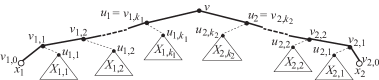
Figure 4: The subtree of $F$ rooted at $v$ in the proof of Lemma 6.6, where thin dashed lines show edges in $B$ and each triangle shows a dangling subtree whose leaf set is a superset of the set inside the triangle.

For each $1\leq j\leq k_{i}$, if $\ell_{F}(X_{i,j})=u_{i,j}$, then $N_{X}(u_{i,j})=0$ (because $N_{X}(v_{i,j})\leq 1$) and hence Lemma 6.4 guarantees that $(T,F)$ has a fair robust key $\kappa_{i,j}=(X_{i,j},B_{i,j})$; otherwise, $N_{X}(\ell_{F}(X_{i,j}))\leq 1$ and hence Lemma 6.4 guarantees that $(T,F)$ has a fair normal key $\kappa_{i,j}=(X_{i,j},B_{i,j})$. So, $\kappa=(X,B_{1}\cup B^{\prime}_{1}\cup B_{2}\cup B^{\prime}_{2},R)$ is a key of $(T,F)$, where $R$ is the edge set of $x_{1}\sim_{F}x_{2}$, $B_{i}=\bigcup_{j=1}^{k_{i}}B_{i,j}$ and $B^{\prime}_{i}=\{e_{F}(u_{i,j})~{}|~{}1\leq j\leq k_{i}\}$ for each $i\in\{1,2\}$.

Note that $|\kappa|=k_{1}+k_{2}+\sum_{i=1}^{2}\sum_{j=1}^{k_{i}}|\kappa_{i,j}|$. Let $\Gamma_{i,j}$ be an $X_{i,j}$-search tree of $(T,F)$ witnessing $b(\kappa_{i,j})$. Obviously, we can use an $X$-search tree $\Gamma$ of $(T,F)$ in which each root-leaf path $P$ can be cut into $2(k_{1}+k_{2})+1$ portions $P_{1,1}$, …, $P_{1,k_{1}}$, $P_{2,1}$, …, $P_{2,k_{2}}$, $Q_{1,1}$, …, $Q_{1,k_{1}}$, $Q_{2,1}$, …, $Q_{2,k_{2}}$, $Q$ (appearing in $P$ in this order), where

• for each $i\in\{1,2\}$ and each $j\in\{1,\ldots,k_{i}\}$, $P_{i,j}$ corresponds to a root-leaf path in $\Gamma_{i,j}$ and $Q_{i,j}$ is a single edge corresponding to picking a cherry $(Y_{i,j},Z_{i,j})$ with $Y_{i,j}\subseteq X_{i,j}$ and $Z_{i,j}\subseteq\bigcup^{j-1}_{h=1}X_{i,h}\cup\{x_{i}\}$,

• $Q$ is a single edge corresponding to picking a cherry $(W_{1},W_{2})$ with $W_{i}\subseteq\bigcup^{k_{i}}_{j=1}X_{i,j}\cup\{x_{i}\}$ for each $i\in\{1,2\}$.

Obviously, the following claims follow from Lemma 6.1:

Claim 1. For each $i\in\{1,2\}$, $Z_{i,1}=\{x_{i}\}$ and for each $j\in\{2,\ldots,k_{i}\}$, either $\ell_{F}(Z_{i,j})$ is a vertex of $x_{i}\sim_{F}v_{i,j}$ other than $v_{i,j}$ or $Z_{i,j}\subseteq X_{i,h}$ for some $h\in\{1,\ldots,j-1\}$.

Claim 2. For each $i\in\{1,2\}$ and each $j\in\{1,\ldots,k_{i}\}$, $f_{e}(\kappa_{i,j},P_{i,j})\subseteq f_{e}(\kappa,P)$ and $f_{c}(\kappa_{i,j},P_{i,j})\subseteq f_{c}(\kappa,P)$. Moreover, for two pairs $\{i,j\}$ and $\{i^{\prime},j^{\prime}\}$ with $\{i,j\}\neq\{i^{\prime},j^{\prime}\}$, $f_{e}(\kappa_{i,j},P_{i,j})\cap f_{e}(\kappa_{i^{\prime},j^{\prime}},P_{i^{\prime},j^{\prime}})=\emptyset$ and $f_{c}(\kappa_{i,j},P_{i,j})\cap f_{c}(\kappa_{i^{\prime},j^{\prime}},P_{i^{\prime},j^{\prime}})=\emptyset$.

Let $A_{e}=\bigcup_{i=1}^{2}\bigcup_{j=1}^{k_{i}}f_{e}(\kappa_{i,j},P_{i,j})$ and $A_{c}=\bigcup_{i=1}^{2}\bigcup_{j=1}^{k_{i}}f_{c}(\kappa_{i,j},P_{i,j})$. By Claims 1 and 2, $A_{e}\subseteq f_{e}(\kappa,P)$, $A_{c}\subseteq f_{c}(\kappa,P)$, $|A_{e}|=\sum_{i=1}^{2}\sum_{j=1}^{k_{i}}|f_{e}(\kappa_{i,j},P_{i,j})|$, and $|A_{c}|=\sum_{i=1}^{2}\sum_{j=1}^{k_{i}}|f_{c}(\kappa_{i,j},P_{i,j})|$. For each $i\in\{1,2\}$ and each $j\in\{1,\ldots,k_{i}\}$, $e_{F}(u_{i,j})\not\in B_{i,j}$ (and hence $e_{F}(u_{i,j})\not\in A_{e}$) because $D_{F}(v_{i,j},\ell_{F}(X_{i,j}))\neq\emptyset$ or $\kappa_{i,j}$ is robust.

Consider an $i\in\{1,2\}$ and a $j\in\{1,\ldots,k_{i}\}$. Further consider the node $\varpi$ of $\Gamma$ at which $P$ picks the cherry $(Y_{i,j},Z_{i,j})$. For convenience, let $T^{\prime}=T\ominus C_{T}$ and $F^{\prime}=F\ominus C(\varpi)$, where $C_{T}$ is the cut of $T$ forced by $C(\varpi)$. By Statement 1 in Lemma 6.1, $\ell_{T^{\prime}}(Y_{i,j})$ agrees with a vertex $w_{i,j}$ of $F^{\prime}$ that is a descendant of $\ell_{F}(X_{i,j})$ in $F$, while $\ell_{T^{\prime}}(Z_{i,j})$ agrees with a vertex $w^{\prime}_{i,j}$ of $F^{\prime}$ that is a descendant of $v_{i,j-1}$ in $F$. Moreover, by Claim 1, either $w^{\prime}_{i,j}$ is a vertex of $x_{i}\sim_{F}v_{i,j-1}$ or $w^{\prime}_{i,j}$ is a descendant of $\ell_{F}(X_{i,h})$ in $F$ for some $h\in\{1,\ldots,j-1\}$. Let $e_{i,j}$ (respectively, $e^{\prime}_{i,j}$) be the edge of $F$ corresponding to $e_{F^{\prime}}(w_{i,j})$ (respectively, $e_{F^{\prime}}(w^{\prime}_{i,j})$).

Claim 3. For each $i\in\{1,2\}$ and each $j\in\{1,\ldots,k_{i}\}$, (1) $f_{c}(\kappa,P)\setminus A_{c}$ contains a component rooted at $u_{i,j}$, (2) $e^{\prime}_{i,j}\in C(P)\cap R$, (3) $e^{\prime}_{i,j}\in C(P)\setminus R$ and either $e^{\prime}_{i,j}\in f_{e}(\kappa,P)\setminus A_{e}$ or $f_{c}(\kappa,P)\setminus A_{c}$ contains a connected component rooted at the head of $e^{\prime}_{i,j}$, or (4) $e_{i,j}\in C(P)\setminus R$ and either $e_{i,j}\in f_{e}(\kappa,P)\setminus A_{e}$ or $f_{c}(\kappa,P)\setminus A_{c}$ contains a connected component rooted at the head of $e_{i,j}$.

To prove Claim 3, consider the three possible ways in which $P$ picks the cherry $(Y_{i,j},Z_{i,j})$. (1) holds when $P$ creates $Y_{i,j}\cup Z_{i,j}$, because of Statement 3 in Lemma 5.7. (2) holds when $P$ isolates $Z_{i,j}$ and $w^{\prime}_{i,j}$ is a vertex of $x_{i}\sim_{F}v_{i,j-1}$. (3) holds when $P$ isolates $Z_{i,j}$ and $w^{\prime}_{i,j}$ is a descendant of $\ell_{F}(X_{i,h})$ in $F$ for some $h\in\{1,\ldots,j-1\}$, because of Lemma 5.6. Similarly, (4) holds when $P$ isolates $Y_{i,j}$.

By Claim 3, each pair $(i,j)$ with $i\in\{1,2\}$ and $j\in\{1,\ldots,k_{i}\}$ contributes at least one element to $(f_{e}(\kappa,P)\setminus A_{e})\cup(f_{c}(\kappa,P)\setminus A_{c})$.

Claim 4. Two different pairs $(i,j)$ and $(i^{\prime},j^{\prime})$ contribute different elements to $(f_{e}(\kappa,P)\setminus A_{e})\cup(f_{c}(\kappa,P)\setminus A_{c})$.

Claim 4 is clearly true when $i\neq i^{\prime}$. So, assume that $i=i^{\prime}$ and $j<j^{\prime}$. If (1) in Claim 3 holds for $(i,j)$, then after $P$ picks $(Y_{i,j},Z_{i,j})$, $e_{F}(u_{i,j})$ cannot be cut by $P$ when picking $(Y_{i,j^{\prime}},Z_{i,j^{\prime}})$. Moreover, if (2) or (3) in Claim 3 holds for $(i,j)$, then after $P$ picks $(Y_{i,j},Z_{i,j})$, $e^{\prime}_{i,j}$ has already been cut by $P$ and hence cannot be cut by $P$ again when picking $(Y_{i,j^{\prime}},Z_{i,j^{\prime}})$. Similarly, if (4) in Claim 3 holds for $(i,j)$, then after $P$ picks $(Y_{i,j},Z_{i,j})$, $e_{i,j}$ has already been cut by $P$ and hence cannot be cut by $P$ again when picking $(Y_{i,j^{\prime}},Z_{i,j^{\prime}})$. Thus, in any case, $(i,j)$ and $(i^{\prime},j^{\prime})$ contribute different elements to $(f_{e}(\kappa,P)\setminus A_{e})\cup(f_{c}(\kappa,P)\setminus A_{c})$, i.e., Claim 4 holds.

By Claims 3 and 4, the $k_{1}+k_{2}$ pairs $(i,j)$ with $i\in\{1,2\}$ and $j\in\{1,\ldots,k_{i}\}$ contributes at least a total of $k_{1}+k_{2}$ elements to $(f_{e}(\kappa,P)\setminus A_{e})\cup(f_{c}(\kappa,P)\setminus A_{c})$. Thus, $b(\kappa,P)\geq k_{1}+k_{2}+\sum_{i=1}^{2}\sum_{j=1}^{k_{i}}b(\kappa_{i,j},P_{i,j})\geq k_{1}+k_{2}+\sum_{i=1}^{2}\sum_{j=1}^{k_{i}}b(\kappa_{i,j})$. Recall that $|\kappa|=k_{1}+k_{2}+\sum_{i=1}^{2}\sum_{j=1}^{k_{i}}|\kappa_{i,j}|$. Since $|\kappa_{i,j}|\leq 2b(\kappa_{i,j})+1$, $|\kappa|\leq 2(k_{1}+k_{2})+2\sum_{i=1}^{2}\sum_{j=1}^{k_{i}}b(\kappa_{i,j})\leq 2b(\kappa,P)$. Because $P$ is an arbitrary root-leaf path of $\Gamma_{X}$, $|\kappa|\leq 2b(\kappa)$. $\Box$

Lemma 6.7

Suppose that $\alpha$ is a semi-close stopper for $(T,F)$. Then, $(T,F)$ has a good abnormal key $\hat{\kappa}=(L_{\alpha},\hat{B},R)$.

Proof. Let $x_{1}$ and $x_{2}$ be as in the definition of a close stopper for $(T,F)$. Let $A$ be the set of $L_{\alpha}$-exclusive edges in $D_{F}(x_{1},x_{2})$. By Lemma 6.6, the lemma holds if $A=\emptyset$. So, we assume that $A\neq\emptyset$. Clearly, we can construct a good abnormal key $\kappa=(L_{\alpha},B,R)$ of $(T,F\ominus A)$ as in the proof of Lemma 6.6. Thus, we hereafter inherit the notations in that proof. Recall that $R$ is the edge set of the path between $x_{1}$ and $x_{2}$ in $F\ominus A$. Further note that the edges in $B$ also appear in $F$.

We set $\hat{B}=B\cup A$. Obviously, $\hat{\kappa}=(X,\hat{B},\hat{R})$ is an abnormal key of $(T,F)$, where $\hat{R}$ is the edge set of $x_{1}\sim_{F}x_{2}$. Since $|\hat{\kappa}|=|A|+k_{1}+k_{2}+\sum_{i=1}^{2}\sum_{j=1}^{k_{i}}|\kappa_{i,j}|$ and $|A|\leq 2$, it remains to show that $b(\hat{\kappa},P)\geq 1+k_{1}+k_{2}+\sum_{i=1}^{2}\sum_{j=1}^{k_{i}}b(\kappa_{i,j},P_{i,j})$. The proof is a simple extension of that of Lemma 6.6. Indeed, the proof of Lemma 6.6 (as it is) already shows that $b(\hat{\kappa},P)\geq k_{1}+k_{2}+\sum_{i=1}^{2}\sum_{j=1}^{k_{i}}b(\kappa_{i,j},P_{i,j})$. We want to show that we can always increase this lower bound by 1. To this end, we take a closer look at (1) in Claim 3 and its proof by distinguishing two cases as follows.

Case 1: $P$ picks $(Y_{i,j},Z_{i,j})$ by creating $Y_{i,j}\cup Z_{i,j}$, and $w_{i,j}\sim_{F}w^{\prime}_{i,j}$ contains the tail of some edge $\hat{e}\in A$. In this case, not only $f_{c}(\kappa,P)\setminus A_{c}$ contains a component rooted at $u_{i,j}$ but also $\hat{e}\in C(P)\cap\hat{B}$.

Case 2: $P$ picks $(Y_{i,j},Z_{i,j})$ by creating $Y_{i,j}\cup Z_{i,j}$, and $w^{\prime}_{i,j}$ is a descendant of $\ell_{F}(X_{i,h})$ in $F$ for some $h\in\{1,\ldots,j-1\}$. In this case, not only $f_{c}(\kappa,P)\setminus A_{c}$ contains a component rooted at $u_{i,j}$ but also $C(P)\cap\hat{R}$ contains the edge entering the child of $v_{i,h}$ that is not an ancestor of $\ell_{F}(X_{i,h})$.

If Case 1 or 2 happens for some $i\in\{1,2\}$ and $j\in\{1,\ldots,k_{i}\}$, then we have increased the lower bound $k_{1}+k_{2}+\sum_{i=1}^{2}\sum_{j=1}^{k_{i}}b(\kappa_{i,j},P_{i,j})$ on $b(\hat{\kappa},P)$ by 1 and hence are done. So, assume that neither Case 1 nor 2 ever occurs. Let $\tilde{e}$ be the edge in $A$ whose tail is the furthest from $v$ in $F$ among the tails of the edges in $A$. Then, there are an $i\in\{1,2\}$ and a $j\in\{0,\ldots,k_{i}\}$ such that the tail of $\tilde{e}$ is an inner vertex of $v_{i,j}\sim_{F}v_{i,j+1}$, where we define $v_{i,k_{i}+1}=v$. We may assume $i=1$.

Now, consider the node $\varrho$ of $\Gamma$ at which $P$ picks the final cherry $(W_{1},W_{2})$. For convenience, let $T^{\prime\prime}=T\ominus C^{\prime}_{T}$ and $F^{\prime\prime}=F\ominus C(\varrho)$, where $C^{\prime}_{T}$ is the cut of $T$ forced by $C(\varrho)$. In the proof of Lemma 6.6, we ignored the contribution of $(W_{1},W_{2})$ to the lower bound $k_{1}+k_{2}+\sum_{i=1}^{2}\sum_{j=1}^{k_{i}}b(\kappa_{i,j},P_{i,j})$ on $b(\hat{\kappa},P)$. So, we here want to count the contribution. For each $i\in\{1,2\}$, let $w_{i}$ be the vertex in $F^{\prime\prime}$ agreeing with $\ell_{T^{\prime\prime}}(W_{i})$ in $T^{\prime\prime}$. Since neither Case 1 nor 2 occurs, either $w_{1}$ is a descendant of $v_{1,j}$ in $F^{\prime\prime}$, or $j<k_{1}$ and $w_{1}$ is a descendant of $\ell_{F}(X_{1,h})$ in $F$ for some $h\in\{j+1,\ldots,k_{1}\}$. In the former case, $\tilde{e}\in D_{F}(w_{1},w_{2})$, implying that $\tilde{e}\in f_{e}(\hat{\kappa},P)$ if $P$ creates $W_{1}\cup W_{2}$. In the latter case, $D_{F}(w_{1},w_{2})$ contains the edge $\ddot{e}$ entering the child of $v_{1,h}$ that is not an ancestor of $u_{1,h}$, implying that $\ddot{e}\in C(P)\cap\hat{R}$ if $P$ creates $W_{1}\cup W_{2}$. On the other hand, if $P$ isolates $W_{i}$ for some $i\in\{1,2\}$, then either $f_{e}(\hat{\kappa},P)$ contains the edge $e^{\prime\prime}_{i}$ of $F$ corresponding to $e_{F^{\prime\prime}}(w_{i})$ or $f_{c}(\hat{\kappa},P)$ contains a component rooted at the head of $e^{\prime\prime}_{i}$. Therefore, in any case, we can increase the lower bound $k_{1}+k_{2}+\sum_{i=1}^{2}\sum_{j=1}^{k_{i}}b(\kappa_{i,j},P_{i,j})$ on $b(\hat{\kappa},P)$ by 1. $\Box$

6.2 The Hard Case

A vertex $\alpha$ of $T$ is an overlapping stopper for $(T,F)$ if $\ell_{F}(L_{\alpha})$ is defined, no descendant of $\alpha$ in $T$ is a semi-close, root, or disconnected stopper for $(T,F)$, and both children $\lambda_{1}$ and $\lambda_{2}$ of $\alpha$ in $T$ are consistent with $F$ but $\alpha$ is not. For example, if $T$ and $F$ are as in Figure 1, then both $\alpha$ and $\beta$ are overlapping stoppers for $(T,F)$.

Lemma 6.8

There always exists a semi-close, root, disconnected, or overlapping stopper for $(T,F)$.

Proof. By assumption, the root in $T$ agrees with no vertex in $F$. So, $T$ has a vertex $\alpha$ such that $\alpha$ is not consistent with $F$ but both children of $\alpha$ are. If some proper descendant of $\alpha$ in $T$ is a semi-close stopper for $(T,F)$, we are done. So, assume that $\alpha$ has no such proper descendant in $T$. Now, if some proper descendant of $\alpha$ in $T$ is a root stopper for $(T,F)$, we are done; otherwise, $\alpha$ must be a disconnected or overlapping stopper for $(T,F)$. $\Box$

So, it remains to show how to compute a good cut for $(T,F)$ when an overlapping stopper for $(T,F)$ exists. The next lemma will be useful later.

Lemma 6.9

Suppose that $\alpha_{1}$ through $\alpha_{k}$ are two or more pairwise incomparable vertices of $T$ satisfying the following conditions:

• For every $i\in\{1,\ldots,k\}$, $\alpha_{i}$ is consistent with $F$ and $N_{L_{\alpha_{i}}}(v)\leq 1$ for each descendant $v$ of $\ell_{F}(L_{\alpha_{i}})$ in $F$.

• $\bigcup^{k}_{i=1}L_{\alpha_{i}}=L_{\alpha}$, where $\alpha=\ell_{T}(\alpha_{1},\ldots,\alpha_{k})$.

• $\ell_{F}(L_{\alpha_{i}}\cup L_{\alpha_{j}})$ is undefined for every pair $(i,j)$ with $1\leq i<j\leq k$.

• Either $\ell_{F}(L_{\alpha_{i}})$ is a root of $F$ for every $i\in\{1,\ldots,k\}$, or neither $\ell_{F}(L_{\alpha_{1}})$ nor $\ell_{F}(L_{\alpha_{2}})$ is a root in $F$.

Then, $(T,F)$ has a good cut $C$ with $\{e_{F}(x)~{}|~{}x\in L_{\alpha}\mbox{ is not a root of }F\}\subseteq C$.

Proof. Let ${\cal I}_{1}$ be the set of all $i\in\{1,\ldots,k\}$ such that $\ell_{F}(L_{\alpha_{i}})$ is a root in $F$ and $|L_{\alpha_{i}}|\geq 2$. Further let ${\cal I}_{2}$ be the set of all $i\in\{1,\ldots,k\}$ such that $\ell_{F}(L_{\alpha_{i}})$ is not a root in $F$. Without loss of generality, we may assume that ${\cal I}_{2}=\{1,2,\ldots,m\}$. For each $i\in{\cal I}_{1}$, we construct a good normal key $\kappa_{i}=(L_{\alpha_{i}},B_{i})$ of $(T,F)$ as in Lemma 6.5. Let $C_{1}=\bigcup_{i\in{\cal I}_{1}}B_{i}$ and $X_{1}=\bigcup_{i\in{\cal I}_{1}}L_{\alpha_{i}}$. By Lemma 6.5, $C_{1}$ is a good cut for $(T,F)$ with $\{e_{F}(x)~{}|~{}x\in X_{1}\}\subseteq C_{1}$. So, we are done if $m=0$. Thus, we may assume that $m\geq 2$. Let $(T^{\prime},F^{\prime})$ be the sub-TF of $(T,F)$ induced by $C_{1}$. Obviously, $F^{\prime}$ is a sub-forest of $F$. Moreover, the conditions in the lemma still hold after replacing $T$, $F$, and $k$ with $T^{\prime}$, $F^{\prime}$, and $m$, respectively. For each $i\in{\cal I}_{2}$, we use Lemma 6.4 to construct a fair normal key $\kappa_{i}=(L_{\alpha_{i}},B_{i})$. Let $C_{2}=\bigcup_{i\in{\cal I}_{2}}B_{i}$ and $X_{2}=\bigcup_{i\in{\cal I}_{2}}L_{\alpha_{i}}$. Now, to show that $C=C_{1}\cup C_{2}$ is desired, it suffices to show that $\kappa=(X_{2},C_{2})$ is a good normal key for $(T^{\prime},F^{\prime})$.

For each $i\in{\cal I}_{2}$, let $\Gamma_{i}$ be an $L_{\alpha_{i}}$-search tree of $(T^{\prime},F^{\prime})$ witnessing $b(\kappa_{i})$. We use an $X_{2}$-search tree $\Gamma$ in which each root-leaf path $P$ can be cut into $m+1$ paths $P_{1}$, …, $P_{m}$, $Q$, where each $P_{i}$ with $i\in{\cal I}_{2}$ corresponds to a root-leaf path in $\Gamma_{i}$. For each $i\in{\cal I}_{2}$, let $Z_{i}$ be the set of $L_{\alpha_{i}}$-descendants of $\ell_{T^{\prime}}(L_{\alpha_{i}})$ in $T^{\prime}-C_{T^{\prime},i}$, where $C_{T^{\prime},i}$ is the cut of $T^{\prime}$ forced by $C(P_{i})$. Further let $e_{i}$ be the edge of $F^{\prime}$ corresponding to $e_{F^{\prime\prime}}(Z_{i})$, where $F^{\prime\prime}=F^{\prime}\ominus C(P_{i})$.

The first edge of $Q$ corresponds to picking a cherry $(Z_{i},Z_{j})$ for some $1\leq i<j\leq m$ such that $\ell_{T^{\prime}}(L_{\alpha_{i}})$ and $\ell_{T^{\prime}}(L_{\alpha_{j}})$ are siblings in $T^{\prime}$. Picking $(Z_{i},Z_{j})$ is done by selecting $h\in\{i,j\}$ and adding $e_{h}$ to $C(P)$; as the result, Lemma 5.6 ensures that either $e_{h}$ becomes an edge in $f_{e}(\kappa,P)$ or $f_{c}(\kappa,P)$ contains a component rooted at the head of $e_{h}$. So, in any case, after picking $(Z_{i},Z_{j})$, $Z_{h^{\prime}}$ will be one part of a cherry for $P$ to pick later, where $h^{\prime}$ is the integer in $\{i,j\}$ such that $e_{h^{\prime}}$ was not added to $C(P)$ when picking $(Z_{i},Z_{j})$; consequently, the next cherry for $P$ to pick is still of the form $(Z_{i^{\prime}},Z_{j^{\prime}})$ for some $1\leq i^{\prime}<j^{\prime}\leq m$. Thus, each edge of $Q$ corresponds to picking a cherry of this form. Moreover, after $P$ finishes picking cherries, there is at most one $g\in{\cal I}_{2}$ such that $e_{g}\not\in C(P)$. Now, $|\kappa|=\sum_{i\in{\cal I}_{2}}|\kappa_{i}|\leq 2\sum_{i\in{\cal I}_{2}}b(\kappa_{i},P_{i})+m$ and $b(\kappa,P)\geq\sum_{i\in{\cal I}_{2}}b(\kappa_{i},P_{i})+(m-1)$. Since $m\geq 2$, $|\kappa|\leq 2b(\kappa,P)$. $\Box$

Hereafter, fix an overlapping stopper $\alpha$ for $(T,F)$. We show how to use $\alpha$ to compute a good cut for $(T,F)$ below. Let $X=L_{\alpha}$, and $X_{1}$ (respectively, $X_{2}$) be the set of leaf descendants of the left (respectively, right) child of $\alpha$ in $T$.

Two leaves $a$ and $b$ are far apart in $F$ if $|D_{F}(a,b)|\geq 3$. Since no descendant of $\alpha$ in $T$ is a semi-close stopper for $(T,F)$, every two leaves in $L_{\alpha}$ are far apart in $F$. The next lemma strengthens Lemma 6.4.

Lemma 6.10

Let $\beta$ be a non-leaf proper descendant of $\alpha$ in $T$. Then, $(T,F)$ has a fair robust key $\kappa=(L_{\beta},B)$ such that if no child of $\ell_{F}(L_{\beta})$ in $F$ is a leaf, $\kappa$ is super-robust.

Proof. For convenience, let $Y=L_{\beta}$. Let $I$ be the set of $Y$-bifurcate vertices in $F$. We claim that for every $v\in I$ with $Y$-children $v_{1}$ and $v_{2}$ in $F$, $(T,F)$ has a fair normal key $\kappa_{v}=(Y^{F}(v),B_{v})$ such that (1) $\kappa_{v}$ is robust, and (2) $\kappa_{v}$ is super-robust if neither $v_{1}$ nor $v_{2}$ is both a leaf and a child of $v$ in $F$. We prove the claim by induction on $|Y^{F}(v)|$. By Lemma 6.3, the claim is true if $|Y^{F}(v)|=2$. So, assume that $|Y^{F}(v)|\geq 3$. We choose an edge $\tilde{e}$ via the robust way of combining $\kappa_{v_{1}}$ and $\kappa_{v_{2}}$. We set $B_{v}=B_{v_{1}}\cup B_{v_{2}}\cup\{\tilde{e}\}$ and $\kappa_{v}=(Y^{F}(v),B_{v})$. By Statement 2 in Lemma 6.2, $|\kappa_{v}|\leq 2b(\kappa_{v})+1$.

Case 1: For some $i\in\{1,2\}$, $v_{i}$ is both a leaf and a child of $v$ in $F$. We may assume $i=1$. Then, $v_{1}\in Y$ by the above crucial point. Moreover, since every two leaves in $Y$ are far apart in $F$, either neither child of $v_{2}$ in $F$ is a leaf, or $|D_{F}(v,v_{2})|\geq 2$ and some child of $v_{2}$ in $F$ is a leaf. In the former case, $\kappa_{v_{2}}$ is super-robust by the inductive hypothesis, and hence $\kappa_{v}$ is robust by the choice of $\tilde{e}$. In the latter case, $\kappa_{v}$ is robust by the choice of $\tilde{e}$.

Case 2: Case 1 does not occur. Then, for each $i\in\{1,2\}$, $D_{F}(v,v_{i})\neq\emptyset$, or $\kappa_{v_{i}}$ is robust by the inductive hypothesis. So, if we can claim that for some $i\in\{1,2\}$, $|D_{F}(v_{i},v)|\geq 2$, $\kappa_{v_{i}}$ is super-robust, or $D_{F}(v,v_{i})\neq\emptyset$ and $\kappa_{v_{i}}$ is robust, then $\kappa_{v}$ is super-robust by the choice of $\tilde{e}$. For a contradiction, assume that the claim is false. Then, for each $i\in\{1,2\}$, either (1) $|D_{F}(v_{i},v)|=1$ and $\kappa_{v_{i}}$ is not robust, or (2) $D_{F}(v,v_{i})=\emptyset$ and $\kappa_{v_{i}}$ is not super-robust. Thus, by the inductive hypothesis, we know that for each $i\in\{1,2\}$, either (1) $|D_{F}(v_{i},v)|=1$ and $v_{i}$ is a leaf, or (2) $D_{F}(v,v_{i})=\emptyset$ and some child of $v_{i}$ in $F$ is a leaf. However, in any case, we found two leaves in $Y$ that are not far apart in $F$, a contradiction. $\Box$

For an $i\in\{1,2\}$, a vertex $\hat{u}$ of $F$ is an $X_{i}$-port if $\hat{u}$ is $X_{i}$-inclusive but $X_{3-i}$-exclusive in $F$, $\hat{u}$ is a non-leaf of $F$, and $e_{F}(\hat{u})\in D_{F}(x_{1},x_{2})$ for some vertices $x_{1}$ and $x_{2}$ in $X_{3-i}$.

Lemma 6.11

Suppose that for some $i\in\{1,2\}$, there is an $X_{i}$-port $\hat{u}$ in $F$. Then, $(T,F)$ has a good normal key.

Proof. We may assume $i=2$. We use Lemma 6.2 to construct a fair normal key $\kappa_{1}=(X_{1},B_{1})$ of $(T,F)$ with $e_{F}(\hat{u})\in B_{1}$. Let $X^{\prime}_{2}=X_{2}^{F}(\hat{u})$. If $|X^{\prime}_{2}|\geq 2$, we use Lemma 6.10 to construct a fair robust key $\kappa_{2}=(X^{\prime}_{2},B_{2})$ of $(T,F)$; otherwise, $X^{\prime}_{2}$ consists of a single $x_{2}\in X_{2}$ and $\kappa_{2}=(X^{\prime}_{2},B_{2})$ with $B_{2}=\{e_{F}(x_{2})\}$. Obviously, no matter what $|X_{2}|$ is, $e_{F}(\hat{u})\not\in B_{2}$. Moreover, $\kappa=(X_{1}\cup X^{\prime}_{2},B)$ with $B=B_{1}\cup B_{2}$ is a normal key of $(T,F)$. We next show that $|\kappa|\leq 2b(\kappa)$.

Clearly, $|\kappa|=|\kappa_{1}|+|\kappa_{2}|\leq 2(b(\kappa_{1})+b(\kappa_{2})+1)$. So, it remains to show that $b_{X}(\kappa)\geq b(\kappa_{1})+b(\kappa_{2})+1$. To this end, we use an $X$-search tree of $(T,F)$ in which each root-leaf path $P$ can be cut into four portions $P_{1}$, $P_{2}$, $Q_{1}$, $Q_{2}$, where $P_{1}$ is a root-leaf path in an $X_{1}$-search tree of $(T,F)$ witnessing $b(\kappa_{1})$, $P_{2}$ is a root-leaf path in an $X^{\prime}_{2}$-search tree of $(T,F)$ witnessing $b(\kappa_{2})$, each edge of $Q_{1}$ corresponds to picking a cherry $(Y,Z)$ with $Y\subseteq X_{2}$ and $Z\subseteq X_{2}$, and $Q_{2}$ consists of a single edge corresponding to picking a cherry $(Y_{1},Y_{2})$ with $Y_{1}\subseteq X_{1}$ and $Y_{2}\subseteq X_{2}$. By Lemma 6.1, $f_{e}(\kappa_{1},P_{1})\cap f_{e}(\kappa_{2},P_{2})=\emptyset$, $f_{c}(\kappa_{1},P_{1})\cap f_{c}(\kappa_{2},P_{2})=\emptyset$, and $f_{c}(\kappa_{2},P_{2})\subseteq f_{c}(\kappa,P)$. Moreover, since $C(P_{1})\cup C(P_{2})\subseteq C(P)$, $f_{e}(\kappa_{1},P_{1})\cup f_{e}(\kappa_{2},P_{2})\subseteq f_{e}(\kappa,P)$. For the same reason, for each $K\in f_{c}(\kappa_{1},P_{1})$, $K$ either remains in $f_{c}(\kappa,P)$ or is split into two or more components in $f_{c}(\kappa,P)$. Thus, $|f_{c}(\kappa_{1},P_{1})|+|f_{c}(\kappa_{2},P_{2})|\leq|f_{c}(\kappa,P)|$. Therefore, $b(\kappa,P)\geq b(\kappa_{1},P_{1})+b(\kappa_{2},P_{2})$. We claim that $b(\kappa,P)\geq b(\kappa_{1},P_{1})+b(\kappa_{2},P_{2})+1$. To see this claim, first note that no component in $f_{c}(\kappa_{1},P_{1})$ is rooted at $\hat{u}$ because each $x\in X^{\prime}_{2}$ is a descendant of $\hat{u}$ in $F-C(P_{1})$. Similarly, no component in $f_{c}(\kappa_{2},P_{2})$ is rooted at $\hat{u}$ because $e_{F}(\hat{u})\not\in B_{2}\cup C(P_{2})$. We next distinguish two cases as follows.

Case 1: $\hat{u}$ has no labeled descendant in $F-(B_{2}\cup C(P_{2}))$. In this case, since $e_{F}(\hat{u})\in B_{1}$, $f_{c}(\kappa,P)$ contains a component rooted at $\hat{u}$. So, $b(\kappa,P)\geq b(\kappa_{1},P_{1})+b(\kappa_{2},P_{2})+1$.

Case 2: $\hat{u}$ has a labeled descendant in $F-(B_{2}\cup C(P_{2}))$. In this case, consider the set $Y_{1}$ of all $x\in X_{1}$ such that $x$ is a descendant of $\ell_{F}(X_{1})$ in $F-C(P_{1})$, and the set $Y_{2}$ of all $x\in X^{\prime}_{2}$ such that $x$ is a descendant of $\ell_{F}(X^{\prime}_{2})$ in $F-C(P_{2})$. By Lemma 6.1, no component in $f_{c}(\kappa_{1},P_{1})$ is rooted at an ancestor of $\ell_{F}(Y_{1})$ in $F$ and no component in $f_{c}(\kappa_{2},P_{2})$ is rooted at a vertex that is both an ancestor of $\ell_{F}(Y_{2})$ in $F$ and a descendant of $\hat{u}$ in $F$. So, if for some $i\in\{1,2\}$, $F-C(P)$ has a component whose leaf set is $Y_{i}$, then we are done because by Lemma 5.6, either $Y_{i}$ consists of a single vertex of $X_{i}$ and $e_{F}(\ell_{F}(Y_{i}))\in f_{e}(\kappa,P)\setminus f_{e}(\kappa_{i},P_{i})$, or $f_{c}(\kappa,P)\setminus f_{c}(\kappa_{i},P_{i})$ contains a component rooted at a vertex that is an ancestor of $\ell_{F}(Y_{i})$ in $F$ (and a descendant of $\hat{u}$ in $F$ if $i=2$). So, we can assume that such $i$ does not exist. Then, $Q_{2}$ must pick the cherry $(Y_{1},Y_{2})$ in the third way and hence $\hat{u}$ is a root of some component in $f_{c}(\kappa,P)$. Therefore, $b(\kappa,P^{\prime})\geq b(\kappa_{1},P_{1})+b(\kappa_{2},P_{2})+1$. $\Box$

By Lemma 6.11, we may hereafter assume that there is neither $X_{1}$-port nor $X_{2}$-port in $F$.

Lemma 6.12

Suppose that for some $h\in\{1,2\}$, $\ell_{F}(X_{h})$ is a descendant of $\ell_{F}(X_{3-h})$ and is $X_{3-h}$-exclusive in $F$. Then, there is a good cut in $F$.

Proof. We may assume $h=2$. Then, $\ell_{F}(X_{1})$ is an ancestor of $\ell_{F}(X_{2})$ in $F$. Further let $v_{1}$, …, $v_{k}$ be those $X_{1}$-bifurcate vertices in $F$ that are also $X_{2}$-inclusive in $F$, where $v_{i}$ is the $X_{1}$-parent of $v_{i-1}$ in $F$ for each $i\in\{2,\ldots,k\}$. Let $v^{\prime}_{0}$ and $v^{\prime}_{1}$ be the $X_{1}$-children of $v_{1}$ in $F$, where $\ell_{F}(X_{2})$ is a descendant of the head of some $\hat{e}\in D_{F}(v^{\prime}_{0},v_{1})$ in $F$. For each $i\in\{2,\ldots,k\}$, let $v^{\prime}_{i}$ be the other $X_{1}$-child of $v_{i}$ in $F$. Since there is no $X_{2}$-port in $F$, $X_{2}$ consists of a single $x_{2}$ and $\hat{e}=e_{F}(x_{2})$. Let $u$ be the tail of $\hat{e}$. See Figure 5.

Figure 5: The subtree of $F$ rooted at $\ell_{F}(X_{1})$ in the proof of Lemma 6.12, where filled triangles show dangling subtrees containing at least one leaf in $X_{1}$, unfilled triangles show dangling subtrees containing no leaf in $X_{1}$, and bold dashed lines show edges in $B$.

It is possible that $v^{\prime}_{0}\in X_{1}$ and $v^{\prime}_{0}$ and $x_{2}$ are siblings in $F$. Suppose that this indeed happens. Then, we can use Lemma 6.4 to construct a fair normal key $\kappa=(X_{1},B)$ of $(T,F)$ with $\hat{e}\in B$. Obviously, $F\ominus B$ has $|F|+|B|$ components. Moreover, since $|\kappa|\leq 2b(\kappa)+1$, $d(T,F\ominus B)\leq d(T,F)-\frac{|B|-1}{2}$. Let $\tilde{F}$ be obtained from $F\ominus B$ by adding back the parent of $v^{\prime}_{0}$ and $x_{2}$ together with $e_{F}(v^{\prime}_{0})$ and $\hat{e}$. Clearly, $d(T,\tilde{F})=d(T,F\ominus B)$ but $|\tilde{F}|=|F\ominus B|-1$. Hence, $|\tilde{F}|-|F|\leq 2(d(T,F)-d(T,\tilde{F}))$. Thus, $(B\setminus\{\hat{e},e_{F}(v^{\prime}_{0})\})\cup\{e_{F}(u)\}$ is a good cut of $F$. So, we hereafter assume that $v^{\prime}_{0}\not\in X_{1}$ or $D_{F}(v^{\prime}_{0},u)\neq\emptyset$.

We use Lemma 6.10 to construct a fair robust key $\kappa=(X_{1},B)$ of $(T,F)$. For each $i\in\{0,1,\ldots,k\}$, consider $\kappa_{i}=(X_{1}^{F}(v^{\prime}_{i}),B_{i})$, where $B_{i}$ is the set of all $e\in B$ such that the head of $e$ is a descendant of $v^{\prime}_{i}$ in $F$. We may assume that $\hat{e}\in B$, because (1) we choose edges via the robust way of combining keys in the construction of $\kappa$, and (2) $D_{F}(v^{\prime}_{0},u)\neq\emptyset$ or $\kappa_{i}$ is a robust key of $(T,F)$. We claim that $\tau=(X_{1},B\cup\{e_{F}(u)\})$ is a normal key of $(T,F)$. Since $v^{\prime}_{0}\not\in X_{1}$ or $D_{F}(v^{\prime}_{0},u)\neq\emptyset$, Lemma 6.10 guarantees that $u$ has a labeled descendant in $F-(B\cup\{e_{F}(u)\})$. Hence, by Lemma 6.10, the claim is true if $v^{\prime}_{1}\not\in X_{1}$, $D_{F}(v^{\prime}_{1},u)\neq\emptyset$, or $X_{1}$ contains neither $v^{\prime}_{2}$ nor a child of $v^{\prime}_{2}$ in $F$. So, assume that $v^{\prime}_{1}\in X_{1}$, $D_{F}(v^{\prime}_{1},u)=\emptyset$, and $X_{1}$ contains $v^{\prime}_{2}$ or a child of $v^{\prime}_{2}$ in $F$. If $v^{\prime}_{2}\in X_{1}$, then $D_{F}(v_{1},v^{\prime}_{2})\geq 2$ (because $v^{\prime}_{1}$ and $v^{\prime}_{2}$ are far apart in $F$) and $B$ contains at most one edge in $D_{F}(v_{1},v^{\prime}_{2})$. On the other hand, if $X_{1}$ contains a child of $v^{\prime}_{2}$ in $F$, then $D_{F}(v_{1},v^{\prime}_{2})\geq 1$ (because every two leaves in $X_{1}$ are far apart in $F$), and in turn Lemma 6.10 guarantees that $B_{2}$ contains one edge in $D_{F}(v_{1},v^{\prime}_{2})$. Therefore, in any case, the component in $F-(B\cup\{e_{F}(u)\})$ containing $v_{1}$ also contains at least one labeled leaf of $F$. Consequently, the claim always holds.

In summary, we have constructed a fair normal key $\kappa=(X_{1},B)$ of $(T,F)$ such that $\hat{e}\in B$ and $\tau=(X_{1},\hat{B})$ with $\hat{B}=B\cup\{e_{F}(u)\}$ is a normal key of $(T,F)$. Let $\Gamma_{1}$ be an $X_{1}$-search tree $\Gamma_{1}$ of $(T,F)$ witnessing $b(\kappa)$. Further let $\Gamma$ be an $X$-search tree of $(T,F)$ in which each root-leaf path $P$ can be transformed into a root-leaf path $P_{1}$ of $\Gamma_{1}$ by deleting the last edge. Let $P$ be an arbitrary root-leaf path in $\Gamma$, and $P_{1}$ be obtained from $P$ by deleting the last edge. Since $\hat{B}$ is a superset of $B$, $f_{e}(\kappa,P_{1})\subseteq f_{e}(\tau,P_{1})$ and $|f_{c}(\tau,P_{1})|\geq|f_{c}(\kappa,P_{1})|$. Moreover, if $u$ has no labeled descendant in $F-(B\cup C(P_{1}))$, then $|f_{c}(\tau,P_{1})|>|f_{c}(\kappa,P_{1})|$ and in turn $b(\tau,P_{1})\geq b(\kappa,P_{1})+1$, implying that $\tau$ is a good key of $(T,F)$ because $|\tau|=|\kappa|+1\leq 2b(\kappa)+2$. Thus, we may assume that $u$ has a labeled descendant in $F-(B\cup C(P_{1}))$. By this assumption, $P_{1}$ never picks a cherry $(Y,Z)$ with $Y\subseteq X^{F}_{1}(u)$ and $Z\cap X^{F}_{1}(u)=\emptyset$ in the third way. Hence, one of the following cases occurs:

Case 1: The set of leaf descendants of $\ell_{F}(X_{1})$ in $F-C(P_{1})$ is a $Y\subseteq X^{F}_{1}(v^{\prime}_{0})$. In this case, the last cherry for $P$ to pick is $(Y,\{x_{2}\})$ and $P$ isolates $Y$ or $\{x_{2}\}$. If $P$ isolates $\{x_{2}\}$, then $\hat{e}\in f_{e}(\tau,P_{1})\setminus f_{e}(\kappa,P_{1})$; otherwise, by Lemma 5.6, $f_{e}(\tau,P)\setminus f_{e}(\kappa,P_{1})\neq\emptyset$ or $f_{c}(\tau,P)\setminus f_{c}(\kappa,P_{1})\neq\emptyset$. So, in any case, $b(\tau,P)\geq b(\kappa,P_{1})+1\geq\frac{1}{2}|\tau|$ and in turn $\tau$ is a good key by Lemma 5.4.

Case 2: The set of leaf descendants of $\ell_{F}(X_{1})$ in $F-C(P_{1})$ is some $Y\subseteq X_{1}\setminus X^{F}_{1}(v^{\prime}_{0})$. In this case, the last cherry for $P$ to pick is $(Y,\{x_{2}\})$ and $P$ isolates $Y$ or $\{x_{2}\}$. By Lemma 6.1, $\ell_{F}(Y)$ is not a root in $F\ominus C(P_{1})$. Thus, as in Case 1, we can prove that $\tau$ is a good key. $\Box$

By Lemma 6.12, we may hereafter assume that for each $i\in\{1,2\}$, $\ell_{F}(X_{i})$ is $X_{3-i}$-inclusive in $F$. By this assumption, $|X_{1}|\geq 2$ and $|X_{2}|\geq 2$. A vertex $v$ in $F$ is a juncture if one child $v_{1}$ of $v$ in $F$ is both $X_{1}$-inclusive and $X_{2}$-inclusive in $F$ and the other $v_{2}$ is $X_{1}$- or $X_{2}$-inclusive in $F$. A juncture $v$ in $F$ is extreme if no proper descendant of $v$ in $F$ is a juncture. Note that $\ell_{F}(X)$ is a juncture in $F$. So, extreme junctures exist in $F$.

Lemma 6.13

$(T,F)$ has a fair normal key $\kappa=(X_{1},B)$ such that $N_{B,X_{2}}(v)\leq 1$ for every descendant $v$ of $\ell_{F}(X_{2})$ in $F$.

Proof. Roughly speaking, the proof is a refinement of that of Lemma 6.4. Let $I$ be the set of $X_{1}$-bifurcate vertices in $F$. The idea is to process the vertices of $I\cup X_{1}$ in a bottom-up fashion. We will maintain an invariant that once a $v\in I\cup X_{1}$ has been processed, we have obtained a fair normal key $\kappa_{v}=(X_{1}^{F}(v),B_{v})$ of $(T,F)$ satisfying the following conditions:

• $\kappa_{v}$ is robust if $N_{X_{1}}(v)=0$.

• $N_{B_{v},X_{2}}(v)=0$ if $v$ has a labeled descendant in $F-B_{v}$.

• $N_{B_{v},X_{2}}(u)\leq 1$ for every descendant $u$ of $v$ in $F$.

We first process each $x\in X_{1}$ by constructing $\kappa_{x}=(\{x\},e_{F}(x))$. We then process those vertices $v\in I$ such that $v$ is $X_{2}$-exclusive in $F$ but its $X_{1}$-parent in $F$ is $X_{2}$-inclusive in $F$, by constructing $\kappa_{v}$ as in the proof of Lemma 6.10; note that $\kappa_{v}$ is robust. Clearly, the invariant is maintained in the two cases. We next describe how to process each $X_{2}$-inclusive $v\in I$. Let $v_{1}$ and $v_{2}$ be the $X_{1}$-children of $v$ in $F$. For each $i\in\{1,2\}$, let $u_{i}$ be the child of $v$ in $F$ that is an ancestor of $v_{i}$ in $F$. We set $\kappa_{v}=(X_{1}^{F}(v),B_{v_{1}}\cup B_{v_{2}}\cup\{\tilde{e}\})$, where $\tilde{e}$ is chosen (in the listed order) as follows:

• If $N_{B_{v_{i}},X_{2}}(u_{i})\geq 1$ for some $i\in\{1,2\}$, then $\tilde{e}=e_{F}(u_{i})$. (Comment: By I2 in the invariant for $v_{i}$, each $X_{2}$-path in $F-B_{v_{i}}$ starting at $u_{i}$ must end at a leaf descendant of the head of some edge in $D_{F}(v,v_{i})$. So, the nonexistence of semi-close stoppers for $(T,F)$ guarantees that $N_{B_{v_{i}},X_{2}}(u_{i})=1$ and $N_{B_{v_{j}},X_{2}}(u_{j})=0$, where $j=3-i$. Thus, I2 in the invariant for $v$ is maintained. Moreover, $\kappa_{v}$ is not robust only when $D_{F}(v,v_{j})=\emptyset$ and $\kappa_{v_{j}}$ is not robust. Hence, by I1 in the invariant for $v_{j}$, $\kappa_{v}$ is not robust only when $N_{X_{1}}(v_{j})\geq 1$ and in turn only when $N_{X_{1}}(v)\geq 1$. So, I1 in the invariant for $v$ is maintained. Because I2 in the invariant hold for both $v_{1}$ and $v_{2}$ and no descendant of $\ell_{T}(X_{2})$ in $T$ is a semi-close stopper for $(T,F)$, I3 in the invariant for $v$ is maintained. By Lemma 6.2, $\kappa_{v}$ is a fair key.)

• If for some $i\in\{1,2\}$, $D_{F}(v,v_{i})=\emptyset$ and $\kappa_{v_{i}}$ is not robust, then $\tilde{e}=e_{F}(u_{3-i})$.

• $\tilde{e}=e_{F}(u_{i})$ for an arbitrary $i\in\{1,2\}$.

Similar to and actually simpler than the above comment on C1, we can also comment on C2 and C3. So, the invariant for $v$ is maintained. We now define $\kappa=(X_{1},B)=\kappa_{r}$, where $r=\ell_{F}(X_{1})$. By the invariant, $\kappa$ is as desired. $\Box$

Lemma 6.14

There is a good cut for $(T,F)$.

Proof. Let $v$ be an extreme juncture in $F$, and $v_{1}$ and $v_{2}$ be the children of $v$ in $F$. Then, for some $i\in\{1,2\}$, both $v_{1}$ and $v_{2}$ are $X_{i}$-inclusive. We may assume $i=1$.

For each $j\in\{1,2\}$, let $x_{j}$ be an $X_{1}$-descendant of $v_{j}$ in $F$. Let $\ddot{X}_{2}$ be the set of all $x\in X_{2}$ such that the head of some edge in $D_{F}(x_{1},x_{2})$ is an ancestor of $x$ in $F$. Since $v$ is $X_{2}$-inclusive in $F$, $\ddot{X}_{2}\neq\emptyset$. Moreover, since $v$ is extreme, no edge in $D_{F}(x_{1},x_{2})$ is both $X_{1}$- and $X_{2}$-inclusive in $F$. So, $e_{F}(x)\in D_{F}(x_{1},x_{2})$ for each $x\in\ddot{X}_{2}$, because otherwise the head of some edge in $D_{F}(x_{1},x_{2})$ would be an $X_{2}$-port in $F$. Furthermore, since $v$ is extreme, there is at most one $x\in\ddot{X}_{2}$ with $e_{F}(x)\in D_{F}(x_{j},v)$ for each $j\in\{1,2\}$. Thus, $1\leq|\ddot{X}_{2}|\leq 2$.

First, consider the case where $|\ddot{X}_{2}|=2$. Because $v$ is extreme, $e_{F}(x_{3})\in D_{F}(x_{1},v)$ for exactly one $x_{3}\in\ddot{X}_{2}$, and $e_{F}(x_{4})\in D_{F}(x_{2},v)$ for exactly one $x_{4}\in\ddot{X}_{2}$. For each $j\in\{1,2\}$, $x_{j}$ and $x_{j+2}$ are siblings in $F$ because otherwise the sibling of $x_{j+2}$ in $F$ would be an $X_{1}$-port. So, by Lemma 5.2, $(T,F)$ has a good normal key and we are done.

We hereafter assume that $\ddot{X}_{2}$ consists of a single vertex $x_{3}\in X_{2}$. Then, there is an $x_{4}\in X_{2}$ that is not a descendant of $v$ in $F$ for $|X_{2}|\geq 2$. So, $e_{F}(x_{j})\in D_{F}(x_{3},x_{4})$ for each $j\in\{1,2\}$, because otherwise the highest $X_{2}$-exclusive ancestor of $x_{j}$ in $F$ would be an $X_{1}$-port in $F$. Thus, for some $h\in\{1,2\}$, $x_{h}$ and $x_{3}$ are siblings in $F$ and $x_{3-h}$ is a child of $v$ in $F$. We may assume that $x_{h}=x_{1}$. Let $w$ be the parent of $x_{1}$ and $x_{3}$ in $F$. Since $v$ is extreme, each edge in $D_{F}(w,v)$ is $X$-exclusive.

We construct a fair normal key $\kappa=(X_{1},B)$ of $(T,F)$ as in the proof of Lemma 6.13. We are lucky if at least one of the following holds:

• For each component $K$ in $F\ominus B$, either the root of $K$ is a leaf or both children of the root of $K$ are $X_{2}$-inclusive in $F\ominus B$.

• $F\ominus B$ has at least two components $K$ such that exactly one child of the root of $K$ is $X_{2}$-inclusive in $F\ominus B$.

Suppose that we are lucky. Then, by Lemma 6.9, we can construct a good normal key $\kappa^{\prime}=(X_{2},B^{\prime})$ of $(T,F\ominus B)$. Let $F^{\prime}=F\ominus(B\cup B^{\prime\prime})$, where $B^{\prime\prime}$ consists of the edges of $F$ corresponding to the edges in $B^{\prime}$. Clearly, $|F^{\prime}|=|F|+|B|+|B^{\prime}|$ and $d(T,F^{\prime})\leq d(T,F)-\frac{|B|+|B^{\prime}|-1}{2}$. We can modify $F^{\prime}$ by adding back $w$ together with $e_{F}(x_{1})$ and $e_{F}(x_{3})$, i.e., by modifying $B\cup B^{\prime\prime}$ by replacing $e_{F}(x_{1})$ and $e_{F}(x_{3})$ with $e_{F}(w)$. The modification decreases $|F^{\prime}|$ by 1 but does not increase $d(T,F^{\prime})$. So, the modified $\hat{B}=B\cup B^{\prime\prime}$ is a cut of $F$ such that $d(T,F\ominus\hat{B})\leq d(T,F)-\frac{1}{2}|\hat{B}|$.

Next, suppose that we are unlucky. Then, $F\ominus B$ has exactly one component $K_{1}$ such that exactly one child of the root of $K_{1}$ is $X_{2}$-inclusive in $F\ominus B$. We want to modify $B$ so that we become lucky without violating the following important condition: $(X_{1},B)$ is a fair normal key of $(T,F)$ and $N_{B,X_{2}}(u)\leq 1$ for all vertices $u$ of $F-B$. In each modification of $B$ below, this important condition will be kept because of the nonexistence of semi-close stoppers for $(T,F)$; so, we will not explicitly mention this fact below.

Recall that $x_{2}$ is a child of $v$ in $F$. So, by C2 in the proof of Lemma 6.13, $e_{F}(v_{1})$ is added to $B$ when we process $v$. Thus, $F\ominus B$ contains a component $K_{2}$ rooted at $v_{1}$. Since $(T,F)$ has no semi-close stopper, $|D_{F}(w,v)|\geq 2$ and in turn one child of $v_{1}$ in $K_{2}$ is $X$-exclusive. Hence, $K_{1}=K_{2}$. We have two ways to modify $B$. One is to replace $e_{F}(v_{1})$ by $e_{F}(x_{3})$ and the other is to replace $e_{F}(v_{1})$ by the edge entering the child of $v_{1}$ that is an ancestor of $x_{1}$ in $F$. If modifying $B$ in the first way does not create a new component $K_{3}$ in $F\ominus B$ such that exactly one child of the root of $K_{3}$ is $X_{2}$-inclusive in $F\ominus B$, then we have become lucky because now $F\ominus B$ satisfies Condition D1; otherwise, we become lucky by modifying $B$ in the second way because now $F\ominus B$ satisfies Condition D2. $\Box$

6.3 Summarizing the Algorithm

We here summarize our algorithm for finding a good cut for $(T,F)$.

1. If there is a sibling-leaf pair $(x_{1},x_{2})$ in $T$ with $|D_{F}(x_{1},x_{2})|=1$, then return $D_{F}(x_{1},x_{2})$.

2. If there is a sibling-leaf pair $(x_{1},x_{2})$ in $F$ such that $|D_{T}(x_{1},x_{2})|=1$ and the head of the unique edge in $D_{T}(x_{1},x_{2})$ is a leaf $x_{3}$, then return $\{e_{F}(x_{3})\}$.

3. If there is a root or disconnected stopper $\alpha$ for $(T,F)$, then compute a good normal key $\kappa=(L_{\alpha},B)$ for $(T,F)$ as in Lemma 6.5, and return $B$.

4. If $(T,F)$ has an overlapping stopper $\alpha$ with children $\beta_{1}$ and $\beta_{2}$ in $T$ such that there is an $L_{\beta_{i}}$-port in $F$ for some $i\in\{1,2\}$, then compute a good normal key $\kappa=(L_{\alpha},B)$ for $(T,F)$ as in Lemma 6.11, and return $B$.

5. If $(T,F)$ has an overlapping stopper $\alpha$ with children $\beta_{1}$ and $\beta_{2}$ in $T$ such that $\ell_{F}(L_{\beta_{i}})$ is a descendant of $\ell_{F}(L_{\beta_{3-i}})$ in $F$ and is $L_{\beta_{3-i}}$-exclusive in $F$ for some $i\in\{1,2\}$, then compute a good cut $C$ for $(T,F)$ as in Lemma 6.12, and return $C$.

6. If there is an overlapping stopper $\alpha$ for $(T,F)$, then compute a good cut $C$ for $(T,F)$ as in Lemma 6.14, and return $C$.

7. Find a semi-close stopper $\alpha$ for $(T,F)$, use $\alpha$ to compute a good abnormal key $\kappa=(L_{\alpha},B,R)$ for $(T,F)$ as in Lemma 6.6, and return $B$.

References

- [1] Baroni, M., Grunewald, S., Moulton, V., and Semple, C. (2005) Bounding the number of hybridisation events for a consistent evolutionary history. Journal of Mathematical Biology, 51, 171-182.
- [2] Beiko, R.G. and Hamilton, N. (2006) Phylogenetic identification of lateral genetic transfer events, BMC Evol. Biol., 6, 159-169.
- [3] Bonet, M.L., John, K. St., Mahindru, R., and Amenta, N. (2006) Approximating subtree distances between phylogenies, Journal of Computational Biology, 13, 1419-1434.
- [4] Bordewich, M., McCartin, C., and Semple, C. (2008) A 3-approximation algorithm for the subtree distance between phylogenies. Journal of Discrete Algorithms, 6, 458-471.
- [5] Bordewich, M. and Semple, C. (2005) On the computational complexity of the rooted subtree prune and regraft distance, Annals of Combinatorics, 8, 409-423.
- [6] Chen, Z.-Z., and Wang, L. (2012) FastHN: a fast tool for minimum hybridization networks, BMC Bioinformatics, 13:155.
- [7] Chen, Z.-Z., and Wang, L. (2013) An ultrafast tool for minimum reticulate networks. Journal of Computational Biology, 20(1): 38-41.
- [8] Chen, Z.-Z., Fan, Y., Wang, L. (2015) Faster exact computation of rSPR distance. Journal of Combinatorial Optimization, 29(3): 605-635.
- [9] Chen, Z.-Z., Machida, E., Wang, L. (2016) An Approximation Algorithm for rSPR Distance. Proceedings of 22nd International Computing and Combinatorics Conference (COCOON’2016), Lecture Notes in Computer Science, Vol. 9797, pp. 468–479, 2016.
- [10] Shi, F., Feng Q., You, J., Wang, J. (2014) Improved Approximation Algorithm for Maximum Agreement Forest of Two Rooted Binary Phylogenetic Trees. To appear in Journal of Combinatorial Optimization.
- [11] Hein, J., Jing, T., Wang, L., and Zhang, K. (1996) On the complexity of comparing evolutionary trees. Discrete Appl. Math., 71, 153-169.
- [12] Ma, B., Wang, L., and Zhang, L. (1999) Fitting distances by tree metrics with increment error. Journal of Combinatorial Optimization, 3, 213-225.
- [13] Ma, B. and Zhang, L. (2011) Efficient estimation of the accuracy of the maximum likelihood method for ancestral state reconstruction. Journal of Combinatorial Optimization, 21, 409-422.
- [14] Maddison, W.P. (1997) Gene trees in species trees. Systematic Biology, 46, 523-536.
- [15] Nakhleh, L., Warnow, T., Lindner, C.R., and John, L.St. (2005) Reconstructing reticulate evolution in species – theory and practice. Journal of Computational Biology, 12, 796-811.
- [16] Rodrigues, E.M, Sagot, M.-F., and Wakabayashi, Y. (2007) The maximum agreement forest problem: Approximation algorithms and computational experiments. Theoretical Computer Science, 374, 91-110.
- [17] Schalekamp, F., van Zuylen, A., and van der Ster, S. (2016) A Duality Based 2-Approximation Algorithm for Maximum Agreement Forest. Proceedings of ICALP 2016, 70:1-70:14.
- [18] Wu, Y. (2009) A practical method for exact computation of subtree prune and regraft distance. Bioinformatics, 25(2), 190-196.
- [19] Whidden, C., Beiko, R. G., and Zeh, N. (2010) Fast FPT algorithms for computing rooted agreement forest: theory and experiments, LNCS, 6049, 141-153.
- [20] Whidden, C. and Zeh, N. (2009) A unifying view on approximation and FPT of agreement forests. LNCS, 5724, 390-401.