On the dimension of triangular self-affine sets
Abstract.
As a continuation of a recent work [6] of the same authors, in this note we study the dimension theory of diagonally homogeneous triangular planar self-affine IFS.
Key words and phrases:
Self-affine measures, self-affine sets, Hausdorff dimension.2010 Mathematics Subject Classification:
Primary 28A80 Secondary 28A781. Introduction
1.1. The theme of the paper
The dimension theory of self-affine measures and sets is so complicated that even on , in the diagonal case (when all the linear part of the mappings from the IFS are diagonal matrices), it is not fully understood. The authors of this note have recently investigated this question [6]. Namely, consider the diagonal self-affine IFS on the plane
| (1) |
The projection of the coordinate axis, naturally generates a self-similar IFS on both coordinate axis. Assume that not both of the similarity dimensions of these projected self-similar IFS are greater than one. In this case, the dimension theory of diagonal self-affine systems on are settled in [6], at least for all but a very small set of parameters.
In this note we make a step forward and consider triangular self-affine IFS. That is we assume that the linear part of the mappings from the IFS are triangular matrices (all of them are lower triangular say). More precisely, let
| (2) |
We say that is diagonally homogeneous if the corresponding diagonal system is homogeneous, that is, all the matrices in (1) are identical. In this case we denote and for all . We mostly investigate the diagonally homogeneous case, see Section 4 and Section 5. However, in the general case, we have result in the case when affinity dimension is smaller than one, see Section 3.
1.2. History
A self-affine Iterated Function System (IFS) is a finite list of contracting affine mappings on . If we choose a ball centered at the origin with sufficiently high radius then this ball will be mapped into itself by all the mappings from the IFS. The ellipses obtained by applying the mappings of the IFS, in any particular order -times, on this ball , are the -cylinders. As tends to infinity, the shapes of many of the -cylinders become more and more relatively thinner and longer. This makes it possible that even if the -cylinders are pairwise disjoint, in some cases, they are not effective covers of the attractor (which is the set that remains after infinite number of iterations of the mappings from the IFS on this ball above).
In 1988 Falconer introduced the notion of affinity dimension [10] for self-affine fractals. We obtain it if we replace the "most economic cover" in the definition of Hausdorff dimension with the most natural cover associated with the -cylinders. In some sense the affinity dimension is the most natural guess for the Hausdorff dimension of a self-affine attractor. Since the affinity dimension of a self-affine IFS
| (3) |
depends only on the linear parts, therefore it remains the same if we substitute with its translations. In 1988 Falconer proved that for almost all translates of a self-affine IFS, the Hausdorff dimension of the attractor and affinity dimension of the IFS are equal, if all of the mappings from the IFS has strong enough contraction. This upper bound on the contractions was originally , which was improved 10 year later by Solomyak [25] to . For a survey of results before 2014 see e.g. [22]. In the last two years there have been a very intensive development on this filed, partially due to the use of Furstenberg measure. See [1], [3], [5], [4], [19], [7], [14].
1.3. Affinity dimension in the triangular case on
In the special case of the triangular self-affine IFS, Falconer and Miao [8, Corollary 2.6] showed that if all the matrices are (e.g. lower) triangular then the affinity dimension can be given explicitly by a formula which depends only on the diagonal elements of the matrices. This formula is rather simple when we are on the plane. Namely, assume that the self-affine IFS is given in the formula (2) and let and be the similarity dimension of the self-similar IFS
| (4) |
respectively. Clearly, is the horizontal and is the vertical projection of the corresponding diagonal system given in the form (1). Let
We define and as the solutions of the following equations:
| (5) |
Then (c.f. [2, Theorem 4.1]) the affinity dimension of is
| (6) |
We say that direction-, (direction-) dominates if , () respectively. It follows from the definition of the Hausdorff dimension that the affinity dimension is always an upper bound for the Hausdorff dimension of the attractor (see [10]).
1.4. Notation
Throughout this note, all self-affine IFS on the plane are supposed to be of the form of (2). Without loss of generality we may assume that
As we mentioned above, the attractor of is
where for . Let be the uniform distribution measure on the symbolic space . That is is the -Bernoulli measure. We define in the natural way.
The push forward measure of is The attractor of the self-similar IFS introduced in (4) is denoted by . The natural projection generated by is
Clearly, , where is the orthogonal projection to the -axis. The measure on the -axis generated by is
| (7) |
Now we introduce the Furstenberg measure. The projection below will be used to construct a method to check that the transversality condition holds.
1.5. Furstenberg measure
In this subsection we study the action of our system on the projective line, in the case
| (8) |
In particular, the direction- dominates.
This action can be identified with the action of a simple iterated function system on the line. Consider the vertical line on the plane. We can identify with . With this identification we define the self-similar IFS on by
| (9) |
(Recall that in this Subsection .) It follows from (8) that all are strict contractions. So, we can define the natural projection in the usual way:
| (10) |
The importance of is as follows: The action of on the projective line is described by the maps
| (11) |
where is .
Then
| (12) |
is the natural projection for .
As a similar construction have first appeared in [12], we will call the projection under of an ergodic measure defined on the Furstenberg measure corresponding to .
1.6. The transversality condition
Consider two cylinders and , . They are parallelograms with two vertical sides. Their angle can be defined as the angle between their non-vertical sides. The following condition holds if any two cylinders and , are either disjoint or have an angle uniformly separated from zero.
Definition 1.1.
We say that satisfies the transversality condition if is there exists a such that for every and for every with we have
| (13) |
Below we present a natural geometric interpretation of this condition which provides a method to check it. First let us define the IFS which acts on
| (14) |
Now we recall two separation properties of IFS. For an IFS we say that it satisfies the Strong Separation Property (SSP) if its natural projection (in case of it is given by ) is a bijection. This is equivalent to the existence of a non-empty open set satisfying
- (a):
-
for all and
- (b):
-
for all ,
where means the closure of the set .
We can define the Open Set Condition (OSC) in an analogous way: an IFS satisfies OSC if there exists a non-empty open set satisfying
- (a):
-
for all and
- (b’):
-
for all ,
Lemma 1.2.
- (i):
-
If satisfies the SSP then the transversality condition holds for .
- (ii):
-
If the transversality condition holds for and for all then satisfies SSP.
Proof.
First we prove part (i). We are going to work with long and thin parallelograms. We will call the principal axis of a parallelogram the direction of its long side.
When ) is a bijection, the usual compactness argument shows that there exists such that for any two symbolic sequences with either
or
Take some . In the first case, for the parallelograms do not intersect at all. In the second case, they intersect but transversally (the angle between their their principal axes is larger than ). In both cases (13) holds. This proves the assertion (i).
Now we prove part (ii). Assume now that (13) holds. By the assumption, there exists such that . Fix some large , to be defined later. Fix also some interval such that for all .
Consider two words with different first digits . Assume for the moment that the parallelograms intersect each other. Then the parallelogram must intersect an internal point of parallelogram , a point which is in distance at least from the vertical boundary and in distance at least from the horizontal (non-vertical) boundary of . Hence, if (13) holds then the angle between the principal axes of the parallelograms is at least . In particular, if was so large that then
| (15) |
On the other hand, when the parallelograms do not intersect each other then (15) also holds. Hence, it holds for all pairs of words with different first digits. This implies that satisfies SSP for the set
This is complete the proof of part (ii) of the assertion. ∎
1.7. Lyapunov exponents, Lyapunov dimension, projection entropy and exponential separation condition
Notation 1.3.
Let be strictly contracting IFS on . Let be the symbolic space, the left-shift operator on and the natural projection is . Let be a probability vector. This generates a Bernoulli measure on , which is denoted by . The corresponding self-similar measure is
| (16) |
Finally, for every we put
| (17) |
1.7.1. Lyapunov exponents and Lyapunov dimension
The general definition of Lyapunov exponents can be found e.g. in [26]. However, in the special case of systems generated by lower triangular matrices like in (2) the vertical direction is preserved by the system. Hence, the Lyapunov exponents can be expressed by the diagonal elements only [8].
The Lyapunov dimension of a self-affine measure was introduced in [1, Definition 1.6]. It is always an upper bound on the Hausdorff dimension of the measure. In the special cases we consider in this note, we can write down a simpler formula for the Lyapunov dimension of :
Example 1.4.
- (a):
-
If is a self-similar IFS on the line then has one Lyapunov exponent which is defined as
(18) - (b):
-
Assume that is a diagonally self-affine IFS on the plane defined as in (1). Then its horizontal and vertical projections of are self-similar IFSs and on the line of the form (4). In this case, has two (not necessarily distinct) Lyapunov exponents: and . We say that direction- dominates if the following counter intuitive condition holds:
(19) Assuming for example that direction- dominates, the Lyapunov dimension can be expressed as
(20) - (c):
1.7.2. Projection entropy
We recall the definition of the projective entropy, which was introduced by Feng and Hu [11].
Here we use Notation 1.3. That is let be a strictly contracting IFS on . Moreover, let be a -invariant ergodic measure on . Let be the partition of , where and we write for the Borel -algebra of . Feng and Hu [11, Definition 2.1] defined the projection entropy of under with respect to
where denotes the usual conditional entropy of given .
1.7.3. Hochman’ exponential separation condition
Hochman introduced the following Diophantine-type condition in [13].
Let be a self-similar IFS on . Let be the minimum of for distinct , where
Condition.
We say that the self-similar IFS satisfies Hochman’s exponential separation condition if there exists an and an such that
| (21) |
We remark that in our earlier paper [6, p.2] we stated this condition in an unnecessarily strict way. Namely, in [6, Condition] we required that (21) holds for all elements of the sequence , while it is enough that this inequality holds only on a subsequence as stated above. However, all the assertions of [6] remain valid under the weaker condition (21) since in [6] we never used the condition directly, we used only the conclusions of Hochman’s Theorems [13].
2. Theorems of Hochman and Feng, Hu
Hochman proved the following very important assertion in [13, Theorem 1.1].
Theorem 2.1 (Hochman).
Here we use Notation 1.3. Let be a self-similar IFS on the real line. Assume that satisfies the Hochman’s exponential separation condition. Let be an arbitrary probability vector.
Then
| (22) |
where .
The ratio on the right hand side of (22) is the similarity dimension of . That is
| (23) |
Theorem 2.2.
Corollary 2.3.
Let be a self-similar IFS on the line which satisfies the Hochman’s exponential separation condition. Then .
Now we consider the diagonally self-affine case on the plane.
Theorem 2.4 (Feng Hu).
Given the diagonally self-affine IFS like in (1). We assume that it satisfies the SSP . Its horizontal and vertical parts (see (4)) are denoted by and .
Fix a probability vector . We consider the Lyapunov exponents and as in (18). Without loss of generality we assume that direction- dominates, which means that
holds. Then
| (25) |
Observe that the Hausdorff dimension of the measure is equal to its Lyaponov dimension if and only if .
3. The trivial case and further notation
3.1. The trivial case
Lemma 3.1.
Assume that direction- dominates and Further, we assume that the exponential separation condition holds for the IFS defined in (4). Then .
The proof is immediate since in this case which is an upper bound always. The lower estimate comes from Hochman Theorem: the dimension of the attractor of is equal to and this attractor is a projection of . Apart from the trivial case, we can get results only if we assume that
| (26) |
3.2. Further notation
We use the notation of Section 1.4.
That is, from now on we always assume that the matrices in (2) are of the form
| (27) |
Clearly, if then direction- dominates and if then direction- dominates.
We use the notation of Section 1.4, where we introduced the uniformly distributed Bernoulli measure on the symbolic space , the natural projection , the projection of to the attractor was called and the projection of to the -axis was denoted by .
The measures and can be disintegrated, according to the partitions
| (28) |
for any sets and . That is the probability measures and are supported by and respectively.
Clearly,
| (29) |
For an arbitrary we write for the restriction of the natural projection to . That is
Then we have and
| (30) |
Now we introduce the vertical distance, vertical ball and and vertical neighborhood of a set:
Further, let
We define the vertical distance in the symbolic space as well:
and are then defined analogously to and .
4. Direction- dominates
In this case by (6),
| (31) |
As we have seen above the case is obvious. So, from now on we may assume that .
Consider the iterated function system . If then the affinity dimension of this system is larger than 1. For systems like that there are many results proving (under different assumptions) that their natural measure is not only absolutely continuous but also has density for some . For example, for Bernoulli convolutions the natural measure has density for almost all parameters ([24]), has density for some for all parameters except a dimension zero subset ([21]), and by the new preprint of Shmerkin it has density for all for all parameters except a dimension zero subset ([20]). It turns out that the knowledge of properties of the density of natural measure is quite useful.
We are going to use the following assumptions:
Assumption A.
(A1) ,
(A2) ,
(A3) with density, for some ,
(A4) satisfies transversality. (Definition 1.1.)
When we replace (A3) with a stronger assumption (B3), we relax our assumption about :
Assumption B.
(B1)
(B2) .
(B3) with density, for all ,
(B4) satisfies transversality.
If we consider the corresponding diagonal system (the one in (1)) then assumptions (A1, B1) say that the similarity dimension to the -axis is greater than one in both cases, while (A2) postulates that the projection to the vertical axis of the corresponding diagonal system has similarity dimension less than one.
Our new results when are as follows:
Theorem 4.1.
Let be a self-affine IFS of the form (2) satisfying Assumption A. Then
| (32) |
Theorem 4.2.
Let be a self-affine IFS of the form (2) satisfying Assumption B. Then
| (33) |
Observe that Assumption A guarantees that .
4.1. The proof of Theorem 4.1
First we give the proof assuming a density assertion (Proposition 4.3). The proof of Proposition 4.3 is given in Sections 4.1.2 and 4.1.3.
4.1.1. The proof of Theorem 4.1 modulo a density lemma
Proof of Theorem 4.1.
Let be the projection entropy which corresponds to the projection (that is, the entropy of ). It follows from [11, Proposition 4.14] that
| (34) |
Observe that . On the other hand, by Assumption (A3), it follows from Corollary 2.3 that we have
| (35) |
Putting these together we obtain that
| (36) |
Our aim below is to prove the corresponding statement for :
| (37) |
Namely, if Proposition 4.3 holds then (37) follows and this implies that for -a.a. we have
| (38) |
Using that we obtain that (38) holds for a set of Hausdorff dimension of . Then by [9, Theorem 5.8] we obtain that
| (39) |
The opposite inequality is immediate since is the affinity dimension of which is always an upper bound on the Hausdorff dimension of the attractor. So, to complete the proof of Theorem 4.1 it is enough to verify Proposition 4.3 below. ∎
4.1.2. Density in the symbolic space versus on the attractor
Proposition 4.3.
For -a.a. we have
| (40) |
The same holds if we replace with on both sides.
We need the following notion:
Definition 4.4 (Definition of ).
Let and we write
| (41) |
where , and for a set , we write for the complement of . We define the function which is the vertical distance from the closest point having a different first cylinder in its symbolic representation:
| (42) |
We say that an is -good if such that for all we have . Moreover, is called good if it is -good for all . That is, we write
| (43) |
The geometric meaning of is given by following observation.
Claim 1.
Assume that is -good for some . Let such that . Then
| (44) |
Proof.
Let . By assumption we have
| (45) |
Using that , and the statement follows from the fact that contracts in vertical direction by factor . ∎
Lemma 4.5.
Let and . Let be a measure on and we write . Then
| (46) |
The equality stays true if we replace by on both sides.
Proof.
Clearly, is supported on . The direction "" follows from the fact that restricted to is a Lipschitz map (with Lipschitz constant 1). This is true for every , hence the inequality in this direction is true for all .
Now we verify the "" part. Fix an an and an which is -good with a constant .
As can be chosen arbitrarily small, the assertion follows. ∎
4.1.3. -almost every point is good
Our goal is to prove
Proposition 4.6.
Let be the uniform distribution on and be defined by (43). Then
| (47) |
Assuming this, we obtain
Recall that, as we discussed above, the proof of Theorem 4.1 follows from Proposition 4.3. So the only thing left is to prove Proposition 4.6. To do so we need the following Lemma. First we introduce
Lemma 4.7.
There exists a constant an such that for all .
| (48) |
Proof.
Let . Then . In the rest of this proof we always suppose that
Recall that by assumption there exist a such that , where is the density function of . It follows from Assumption (A2) that we can choose a such that
| (49) |
and let
and
It follows from Corollary 7.5 of the Appendix that
| (50) |
where is a constant. Furthermore by Markov inequality
that is
| (51) |
Now we define
| (52) |
We define
| (53) |
That is consist of those elements of which are "bad" because of . It follows from transversality (Definition 1.1 ) that
| (54) |
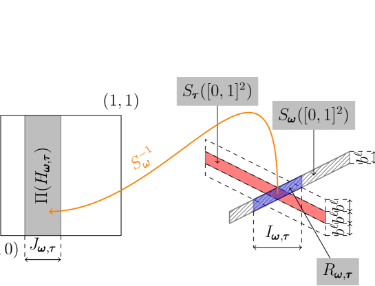
Let
The importance of is that it follows from elementary geometry that
| (55) |
It follows from the construction of that there is a (possibly empty) interval such that
where the length of the interval
| (56) |
Let
Hence the concatenation of and is
| (57) |
To shorten the notation for an we define
| (58) |
To estimate we present
where
It follows from the definition of the set that
| (61) |
On the other hand, it follows from the definition of that
| (62) |
∎
Corollary 4.8.
Let Then .
The Proposition 4.6 is now immediate:
4.2. density case
In this section we will give the proof of Theorem 4.2. In this subsection we assume that is absolute continuous with density for all , we also assume the transversality condition.
In the previous subsection we proved Lemma 4.7. In the calculation of we were not able to make use of the following fact: if the intervals and intersect for some , it does not necessarily mean that the parallelograms and intersect as well. Under the assumption this distinction can be made.
4.2.1. Number of pairs of intersecting cylinder parallelograms
In this subsection we give an upper bound on the number of intersecting (or close-by) level cylinders with distinct first coordinates. To state the lemma we need some preparation.
We write
| (65) |
For an and let
| (66) |
Further, for we write
| (67) |
where was defined in (53) and
| (68) |
Note that by transversality
| (69) |
Let
| (70) |
Lemma 4.9.
Assume that Conditions (B1), (B3) and (B4) hold. Then for every
Proof.
Choose some . Let . Let us define a finite sequence as follows: and
| (71) |
Let . Naturally,
We show that for every there exists such that for every
| (72) |
Let . Assume that
| (73) |
Observe that this is possible only if both
- (a):
-
and
- (b):
-
and
Hence by Corollary 7.6, for every there are at most words such that . In the same way there are at most words such that . So, taking into consideration condition (a) above, we obtain (72).
Thus, by induction
But by definition of the sequence , , , and there exist constants such that . Therefore,
and passing with to infinity proves the assertion. ∎
4.2.2. The corellation dimension
First we recall the definition of the correlation dimension (see [16]).
Definition 4.10.
Let be a positive bounded regular Borel measure on with bounded support . For every let be the -mesh cubes that intersect . For a , we define
| (74) |
Equivalently we could define (see [16]) in either of the following two ways: let
| (75) |
Then
| (76) |
For the -dimension of is defined as
| (77) |
It was proved by Hunt and Kaloshin [15, Proposition 2.1] that
| (78) | ||||
If we apply this for we get the correlation dimension of the measure
It follows from (78) that
| (79) |
Proof of Theorem 4.2.
We will prove that under Assumption B
Let and consider the grid of size . Let be one of the -mesh cubes. Let be such that intersects . Then is contained in some vertical strip of width , hence by Corollary 7.6
Let be an upper bound on the maximal slope of (the principal axis of) our cylinders. Then if the cylinder intersects , it must also intersect at least one of vertical intervals: either or . Let us denote the number of cylinders intersecting by and the number of cylinders intersecting by . Using a similar estimate as in the proof of Lemma 4.7, in equation (4.1.3) we can write
hence
Thus,
where is the -th -mesh cube. It is enough to estimate the first sum, the second is analogous. The interval intersects if and only if the point is contained in . Hence, is equal to the number of pairs such that contains .
For every we write . Then for , there exists such that
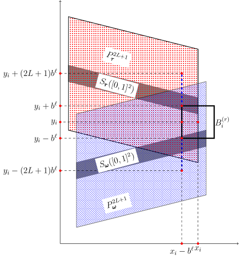
With this notation we present this sum as
Given , the last sum can be estimated by
| (80) |
Namely, by the Transversality Condition we can apply
(69) which yields that
and
. Thus we have only different ’s in and for each of them we have at most different ’ in . Then (80) follows from
(70).
Applying Lemma 4.9 and noting that can take values, we get
The last sum is a geometric series, hence it is bounded by a constant when and by when . When this sum equals . Thus,
Passing with to infinity and to 0 we get
∎
5. Direction- dominates
Finally, in this section we turn to the case when the direction- dominates. In this direction, we have only a mild development on the way of understanding the overlapping self-affine systems. The result can be considered as an extension of [6, Theorem B] and [3, Theorem 4.8, Theorem 4.11].
Similarly to the Section 1.5, we define the backward Furstenberg measure and IFS. This measure is supported on the directions, associated to the strong-stable directions. We note that in the case, when direction- dominates, the backward Furstenberg measure is supported on the singleton .
Consider again the vertical line on the plane and identify with . Moreover, let be the self-similar IFS on defined by
| (81) |
Let us define the natural projection by in the usual way:
| (82) |
Similarly, to (12), we have that the action of on the projective line is described by the maps
where is .
Assumption C.
We assume that
(C1) ,
(C2)
(C3) The backward Furstenberg IFS satisfies Hochman’s exponential separation condition,
(C4) satisfies Hochman’s exponential separation condition,
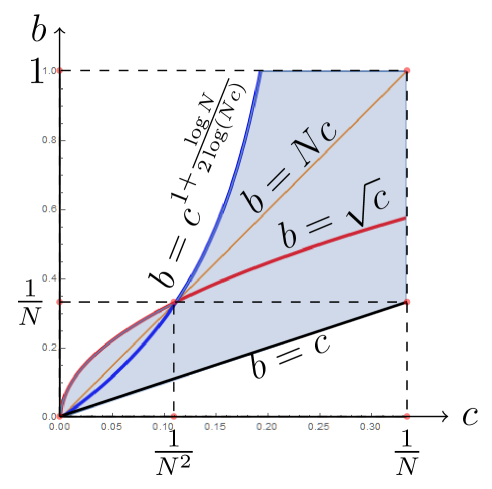
Conditions (C1) and (C4) are devoted to be able to handle the projection entropy (defined in Section 1.7.2). Condition (C3) allows us to calculate the dimension of the backward Furstenberg measure and condition (C5) ensures that its dimension is larger than some possible exceptional set of orthogonal projections, for which the dimension drops.
Theorem 5.1.
Let be a self-affine IFS of the form (2) satisfying Assumption C. Then
| (83) |
As previously, let be the uniform Bernoulli measure on the symbolic space and let be its projection by the mapping , defined in Section 1.4.
For proper subspace of , let us denote the orthogonal projection from to the subspace (orthogonal subspace to ) by . By [4, Theorem 2.2],
| (84) |
where is the projection entropy, defined in Section 1.7.2.
Lemma 5.2.
If (C1), (C2) and (C4) in Assumption C hold then .
Proof.
Let us define a lifted IFS on and a derived IFS on , as follows
where and are chosen such that
| (85) |
Denote the natural projections of and by and respectively. Let us define and the push-down measures.
We note that the Lyapunov exponents coincide for every measure , and for the appropriate directions. Applying [4, Corollary 2.9] and [11, Theorem 2.11], we have
| (87) | |||||
| (88) |
| (89) |
Let us introduce measurable partitions of by and . Moreover, define a measurable partition of by and a measurable partition of by .
By Rokhlin’s Theorem there are families of conditional measures , , and on the partitions respectively, uniquely defined up to zero measure sets.
By definition of conditional measures and the partition , , where , see (29). On the other hand, . Thus,
Let be the orthogonal projection to the -coordinate plane. Since for -a.e. , we get that
| (90) |
Applying [4, Theorem 7.1] we have
By assumptions (C1) and (C4), we may apply [11, Theorem 2.8] and [13, Theorem 1.1], and therefore
Therefore for -a.e. .
By (90), if for a Borel set then for -a.e . Thus, by the definition of the Hausdorff dimension for -a.e . Hence for -a.e. , which implies that . ∎
Lemma 5.3.
Let be a self-affine IFS of the form (2) satisfying the assumptions of Assumption C. Then
| (91) |
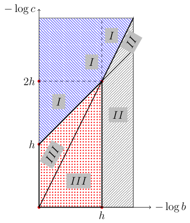
Proof.
6. Examples
6.1. Examples for the direction- dominates case
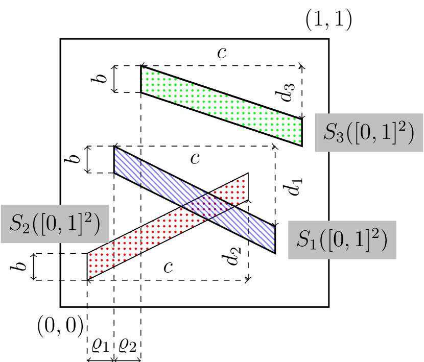
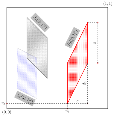
We present three examples. In the first and second case we can apply Theorem 4.1 and in the third example we can apply Theorem 4.2. In all examples can be chosen as an arbitrary element of a parameter interval except a small exceptional set which is going to be , and in the examples respectively with the properties:
| (95) |
The precise definition of these exceptional sets are given in Section 6.1.2.
Example 6.1.
We can apply Theorem 4.1 in Example 6.1 because Assumption A holds. Namely, it is obvious that assumptions (A1)-(A2) hold. Assumption (A3) follows from choice of (see (105)). Assumption (A4), (the transversality condition) follows from the fact that the associated -dimensional IFS , defined in (14), satisfies SSP. Namely, the third coordinate of is an IFS on the line, defined in (9). This consists of two maps with distinct fixed points and the sum of their contraction ratios is less than . This means that the SSP holds for . Consequently, the SSP holds for . Hence the transversality condition (A4) also holds.
Example 6.2.
- (a):
-
.
- (b):
-
We fix an arbitrary . (See (106).)
- (c):
-
Let .
- (d):
-
are pairwise different.
- (e):
-
We assume that and we choose from the interval
Note that this holds for example if .
- (f):
-
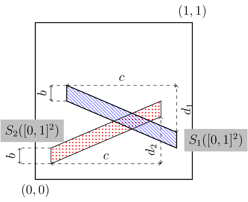
We choose the vertical translation parameters (like on the right hand side of Figure 5(b)) so that
(97) and for .
Then we have
| (98) |
(See Figure 5(b).)
Example 6.3.
- (a):
-
.
- (b):
-
We fix an arbitrary . (See (106).)
- (c):
-
Let .
- (d):
-
are consecutive elements of an arithmetic progression (not necessarily in this order).
- (e):
-
We assume that and we choose from the interval
Note that this holds for example if .
- (f):
-
We choose the vertical translation parameters (like on the right hand side of Figure 5(b)) so that
(99) and for .
Then we have
| (100) |
(See Figure 5(b).)
Combining (c), (e) and (f) (note that these assumptions appear both in Examples 6.2 and 6.3) we get that the transversality condition holds. Namely, with the open set
the IFS satisfies the SSP. Hence by Lemma 1.2 the transversality condition holds. Hence, we can apply Theorem 4.1 for Example 6.2 in the same way we applied it for the Example 6.1.
For the example 6.3 we are going to apply Theorem 4.2 here. The combination of (b) and Corollary 6.5 implies that has bounded density. Hence, Theorem 4.2 applies.
6.1.1. Phase transition in Example 6.3
Note that in Example 6.3 the parameter interval can be partitioned naturally into
Namely, the affinity dimension
is monotone increasing in both and . So, for a fixed it takes its biggest value for . Clearly is the solution of That is for we have for every . However, for it depends on the choice of if or . Now we fix a , and satisfying the conditions of Example 6.3. We vary only . So, the attractor will be denoted by . To study the function
| (101) |
first observe that for a the function is monotone increasing and
| (102) |
That by Theorems 4.2, for a we have:
| (103) |
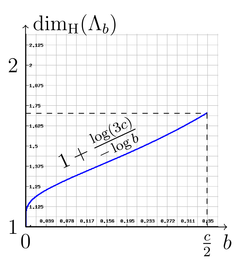
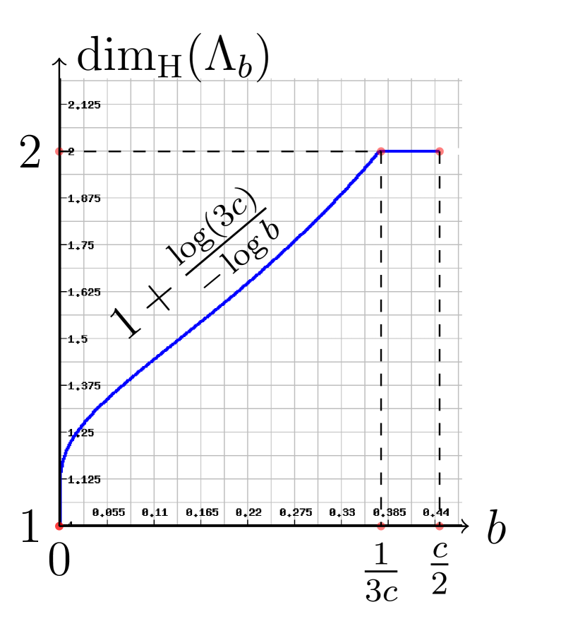
Which means that there is a phase transition at , where the graph of is non-differentiable, although it is continuous on the interval .
6.1.2. The definition of exceptional parameter sets .
Let be the set of exceptional parameters
| (104) |
Let
| (105) |
It follows from [21, Theorem A] that and are sets of Hausdorff dimension zero. About note that as long as the exceptional set is the same for all IFS .
To define the third exceptional set first we need to state the following theorem [23, Theorem 2]
Theorem 6.4 (Simon, Tóth).
For a natural number let be the self-similar measure corresponding to the IFS and the uniform distribution of weights . Then there exists an exceptional set having Lebesgue measure zero such that is absolute continuous with density whenever .
From this is is immediate to see that the following Corollary holds:
Corollary 6.5.
Here we use the notation of Theorem 6.4. Let
| (106) |
Then the Lebesgue measure of is zero and is absolutely continuous with continuous (consequently bounded) density for each .
6.2. Example for the direction- dominates case
Before we show an example for Theorem 5.1, we show a family of IFS of similarities, which satisfies Hochman’s exponential separation condition.
Lemma 6.6.
Let be an IFS on the real line such that , and . Then satisfies Hochman’s exponential separation condition.
The proof is similar to the proof of [13, Theorem 1.6].
Proof.
Without loss of generality, we may assume that , and irrational. For any finite length word , let
By (21), it is enough to show that there exists and a sequence such that for any with , . Suppose that this is not the case. That is, for every there exists a such that for every there exist finite words with such that
| (107) |
By definition, , where relative primes and . Thus, for any with ,
where . Observe that
for every and with . On the other hand, if and then , because of the rational root test of polynomials with integer coefficients. Thus, .
Example 6.7.
7. Appendix
Here we collect some consequences of the fact that a measure on the line is absolute continuous with density for a .
Given a measure supported by and we assume that there exists a such that the density of satisfies:
| (109) |
Lemma 7.1.
Let be the density of . Assume that (109) holds. Then for any interval
Proof.
By Jensen’s inequality we have
| (110) |
This completes the proof after some obvious algebraic manipulations. ∎
Definition 7.2.
Given a real number . We say that a not necessarily countable family , of closed intervals is an -bad family if
| (111) |
We say that is a disjoint -bad family of intervals if is an -bad family and the intervals in are pairwise disjoint.
Lemma 7.3.
There exists a constant independent of everything such that for every if is an -bad family of intervals then
| (112) |
Proof for disjoint -bad families.
Proof for non-disjoint -bad families.
Fix an . For every and for every let
Let and we form the family of closed (one dimensional) balls . Then by definition we can apply Besicovitch’s covering theorem (using the notation of [17, p. 30, Theorem 2.7 part (2)]) for and . From this theorem there is a constant independent of everything such that we can find sub-families of such that
- (a):
-
for every , is a disjoint family. That is for any two distinct intervals we have .
- (b):
-
If then for some and . Then
(115) - (c):
-
.
Using (a) and (b) for every , is a disjoint -bad family. Since we have already verified the assertion of the lemma for disjoint families we can apply (114) for (with writing instead of ) to get that for all :
| (116) |
Using this and (c) above we obtain that
| (117) |
∎
From we get the following two corollaries:
Corollary 7.4.
Let be a family of intervals of and . Then . So,
| (118) |
Corollary 7.5.
Corollary 7.6.
Assume has density for all . Then for every and there exists such that for every every interval of length intersects at most intervals .
Proof.
Denote by the number of intervals intersecting . Each of those intervals is contained in the interval . Hence,
Applying Lemma 7.1 to the interval we get the assertion. ∎
References
- [1] B Bárány, Mark Pollicott, and K Simon. Stationary measures for projective transformations: the blackwell and furstenberg measures. Journal of Statistical Physics, 148(3):393–421, 2012.
- [2] Balázs Bárány. Dimension of the generalized 4-corner set and its projections. Ergodic Theory and Dynamical Systems, 32(04):1190–1215, 2012.
- [3] Balázs Bárány. On the Ledrappier-Young formula for self-affine measures. Math. Proc. Cambridge Philos. Soc., 159(3):405–432, 2015.
- [4] Balázs Bárány and Antti Käenmäki. Ledrappier-young formula and exact dimensionality of self-affine measures. arXiv preprint arXiv:1511.05792, 2015.
- [5] Balázs Bárány and Michał Rams. Dimension maximizing measures and local dimension spectrum for self-affine systems. arXiv preprint arXiv:1507.02829, 2015.
- [6] Balázs Bárány, Michał Rams, and Károly Simon. On the dimension of self-affine sets and measures with overlaps. Proceedings of the American Mathematical Society, 2016.
- [7] Kenneth Falconer and Tom Kempton. The dimension of projections of self-affine sets and measures. arXiv preprint arXiv:1511.03556, 2015.
- [8] Kenneth Falconer and Jun Miao. Dimensions of self-affine fractals and multifractals generated by upper-triangular matrices. Fractals, 15(03):289–299, 2007.
- [9] Kenneth J Falconer. The geometry of fractal sets, volume 85. Cambridge university press, 1986.
- [10] Kenneth J Falconer. The hausdorff dimension of self-affine fractals. Math. Proc. Camb. Phil. Soc, 103(3):339–350, 1988.
- [11] De-Jun Feng and Huyi Hu. Dimension theory of iterated function systems. Communications on Pure and Applied Mathematics, 62(11):1435–1500, 2009.
- [12] H. Furstenberg and Y. Kifer. Random matrix products and measures on projective spaces. Israel J. Math., 46(1-2):12–32, 1983.
- [13] Michael Hochman. On self-similar sets with overlaps and inverse theorems for entropy. Ann. of Math. (2), 180(2):773–822, 2014.
- [14] Michael Hochman and Boris Solomyak. On the dimension of furstenberg measure for random matrix products. arXiv preprint arXiv:1610.02641, 2016.
- [15] Brian R. Hunt and Vadim Yu. Kaloshin. How projections affect the dimension spectrum of fractal measures. Nonlinearity, 10(5):1031–1046, 1997.
- [16] Ka-Sing Lau. Self-similarity, -spectrum and multifractal formalism. In Fractal geometry and stochastics (Finsterbergen, 1994), volume 37 of Progr. Probab., pages 55–90. Birkhäuser, Basel, 1995.
- [17] Pertti Mattila. Geometry of sets and measures in Euclidean spaces: fractals and rectifiability. Number 44. Cambridge University Press, 1999.
- [18] Yuval Peres and Wilhelm Schlag. Smoothness of projections, Bernoulli convolutions, and the dimension of exceptions. Duke Math. J., 102(2):193–251, 2000.
- [19] Ariel Rapaport. On self-affine measures with equal hausdorff and lyapunov dimension. arXiv preprint arXiv:1511.06893, 2015.
- [20] Pablo Shmerkin. On furstenberg’s intersection conjecture, self-similar measures, and the norms of convolutions. arXiv preprint arXiv:1609.07802, 2016.
- [21] Pablo Shmerkin and Boris Solomyak. Absolute continuity of self-similar measures, their projections and convolutions. arXiv preprint arXiv:1406.0204, 2014.
- [22] Károly Simon. The dimension theory of almost self-affine sets and measures. In Fractals, Wavelets, and their Applications, pages 103–127. Springer, 2014.
- [23] Károly Simon and Hajnal R. Tóth. The absolute continuity of the distribution of random sums with digits . Real Anal. Exchange, 30(1):397–409, 2004/05.
- [24] Boris Solomyak. On the random series (an erdös problem). Annals of Mathematics, 142(3):611–625, 1995.
- [25] Boris Solomyak. Measure and dimension for some fractal families. In Mathematical Proceedings of the Cambridge Philosophical Society, volume 124, pages 531–546. Citeseer, 1998.
- [26] Peter Walters. An introduction to ergodic theory, volume 79 of Graduate Texts in Mathematics. Springer-Verlag, New York-Berlin, 1982.
