A generalized bayesian inference method for constraining the interiors of super Earths and sub-Neptunes

Abstract

Aims. We aim to present a generalized Bayesian inference method for constraining interiors of super Earths and sub-Neptunes. Our methodology succeeds in quantifying the degeneracy and correlation of structural parameters for high dimensional parameter spaces. Specifically, we identify what constraints can be placed on composition and thickness of core, mantle, ice, ocean, and atmospheric layers given observations of mass, radius, and bulk refractory abundance constraints (Fe, Mg, Si) from observations of the host star’s photospheric composition.

Methods. We employed a full probabilistic Bayesian inference analysis that formally accounts for observational and model uncertainties. Using a Markov chain Monte Carlo technique, we computed joint and marginal posterior probability distributions for all structural parameters of interest. We included state-of-the-art structural models based on self-consistent thermodynamics of core, mantle, high-pressure ice, and liquid water. Furthermore, we tested and compared two different atmospheric models that are tailored for modeling thick and thin atmospheres, respectively.

Results. First, we validate our method against Neptune. Second, we apply it to synthetic exoplanets of fixed mass and determine the effect on interior structure and composition when (1) radius, (2) atmospheric model, (3) data uncertainties, (4) semi-major axes, (5) atmospheric composition (i.e., a priori assumption of enriched envelopes versus pure H/He envelopes), and (6) prior distributions are varied.

Conclusions. Our main conclusions are: (1) Given available data, the range of possible interior structures is large; quantification of the degeneracy of possible interiors is therefore indispensable for meaningful planet characterization. (2) Our method predicts models that agree with independent estimates of Neptune’s interior. (3) Increasing the precision in mass and radius leads to much improved constraints on ice mass fraction, size of rocky interior, but little improvement in the composition of the gas layer, whereas an increase in the precision of stellar abundances enables to better constrain mantle composition and relative core size. (4) For thick atmospheres, the choice of atmospheric model can have significant influence on interior predictions, including the rocky and icy interior. The preferred atmospheric model is determined by envelope mass.

This study provides a methodology for rigorously analyzing general interior structures of exoplanets which may help to understand how exoplanet interior types are distributed among star systems. This study is relevant in the interpretation of future data from missions such as TESS, CHEOPS, and PLATO.

1 Introduction

The characterization of planet interiors is one of the main foci of current exoplanetary science. For the characterization of super Earths and sub-Neptunes, we mostly rely on mass and radius measurements. Direct measurements of atmospheres are, thus far, mostly limited to transiting hot Jupiters and a few Sub-Neptunes (Iyer et al., 2015), with the exception of super Earth 55 Cnc E (Tsiaras et al., 2016; Demory et al., 2016). For interior characterization, common practice is the use of mass-radius-plots where mass and radius of exoplanets are compared to synthetically computed interior models (e.g., Sotin et al., 2007; Seager et al., 2007; Fortney et al., 2007; Dressing et al., 2015; Howe et al., 2014). However, it is difficult to know (1) how well one interior model compares with the generally large number of other possible interior scenarios that also fit data and (2) which structural parameters can actually be constrained by the observations. Thus, this approach fails to address the degeneracy problem that is, that different interior models can have identical mass and radius. In order to draw meaningful conclusions about an exoplanet’s interior it is therefore necessary to account for this inherent degeneracy (e.g., Rogers & Seager, 2010; Schmitt et al., 2014; Carter et al., 2012; Weiss et al., 2016; Dorn et al., 2015).

The Bayesian analysis of Rogers & Seager (2010) to exoplanets of three to four parameters was generalized for purely rocky exoplanets by Dorn et al. (2015). Here, we extend the full probabilistic analysis of Dorn et al. (2015) to more general interior structures by including volatile elements in form of icy layers, oceans, and atmospheres. The previous work of Rogers & Seager (2010) uses a grid search method which calls for strong a priori assumptions on structure and composition of exoplanets to significantly reduce the parameter space. However, the number of parameters that affect mass and radius is large (e.g., it comprises composition and size of core, mantle, ice layers, and gas, as well as internal energy). Here, we present a generalized Bayesian inference scheme that incorporates the following aspects:

• Our method is applicable to a wide range of planet-types, including rocky super Earths and sub-Neptunes.

• We employ a full probabilistic Bayesian inference analysis using a Markov chain Monte Carlo (McMC) technique to constrain core size, mantle thickness and composition, mass of water-ice, and key characteristics of the atmosphere (e.g., mass, intrinsic luminosity, composition).

• We test two different atmospheric models, tailored to thick and thin atmospheres, that account for enrichments in elements heavier than H and He.

• We employ state-of-the-art modeling to compute interior structure based on self-consistent thermodynamics for a pure iron core, a silicate mantle, high-pressure ice, water ocean, and atmosphere (to some extent).

• Compared to previous work of Rogers & Seager (2010), our scheme can also be used for high dimensional parameter spaces.

Besides mass and radius estimates, additional constraints are crucial to reduce model degeneracy (e.g., Dorn et al., 2015; Grasset et al., 2009). Dorn et al. (2015) demonstrate that the use of relative bulk abundance constraints of Fe/Si and Mg/Si taken from the host star (henceforth referred to as abundance constraints) leads to much improved constraints on core size and mantle composition in the case of purely rocky exoplanets. The validity of a direct correlation between stellar and planetary relative bulk abundances is suggested by observational solar system studies and planet formation models (Carter et al., 2012; Lodders, 2003; Drake & Righter, 2002; McDonough & Sun, 1995; Bond et al., 2010; Elser et al., 2012; Johnson et al., 2012; Thiabaud et al., 2015). Here, we also assume solar bulk abundance constraints based on spectroscopic measurements (Lodders, 2003).

Our generalized interior structure model is based on previous studies of mass-radius relations. Generally, H₂O in liquid and high-pressure ice form (e.g., Valencia et al., 2007a; Seager et al., 2007), and H₂-He atmospheres (e.g., Rogers et al., 2011; Fortney et al., 2007) are considered. Although it would not be surprising if the compositional diversity of ices and atmospheres exceeds the one found in the solar system (e.g., Newsom, 1995), the few observational data on exoplanets limit us to relatively simple planetary interior models.

The structural parameters that we investigate include: (1) internal energy, mass, and composition of the gas layer, (2) mass and temperature of the ice layer, (3) mantle size and composition, and (4) core size. For present purposes, we assume a general planetary structure consisting of a pure iron core, a silicate mantle, a water ice layer and an atmosphere. To compute the resultant density profile for the purpose of estimating mass and radius, we follow Dorn et al. (2015) and assume hydrostatic equilibrium coupled with a thermodynamic approach based on Gibbs free-energy minimization and Equation-of-State (EoS) modeling.

In this study, we wish to quantify the influence of the following parameters on predicted interior structure and composition: (1) planet radius, (2) data uncertainty (e.g., mass, radius, bulk abundances), (3) semi-major axis, (4) atmospheric model, (5) atmospheric composition (i.e., a priori assumption of enriched envelopes versus pure H/He envelopes), and (6) prior distributions. In a companion paper (Dorn et al., 2017), we present results on the application of our proposed method to six exoplanets (HD 219134b, Kepler-10b, Kepler-93b, CoRoT-7b, 55 Cnc e, and HD 97658b) for which spectroscopic measurement of their host star’s photospheres are available (Hinkel et al., 2014).

The outine of this study is as follows: we describe the iterative inference scheme (Section 2.1), model parameters (Section 2.2), data (Section 2.3), and the forward model (Section 2.4). In Section 3, we validate our method against Neptune and present results for different synthetic planet cases. In Sections 4 and 5, we discuss results and conclude.

2 Methodology

2.1 Bayesian inference

We employ a Bayesian method to compute the posterior probability density function (pdf) for each model parameter m from data d and prior information. According to Bayes’ theorem, the posterior distribution ${\rm p}({\bf m}|{\bf d})$ for a fixed model parameterization, conditional on data, is proportional to prior information ${\rm p}({\bf m})$ on model parameters and the likelihood function ${\rm L}({\bf m}|{\bf d})$, which can be interpreted in probabilistic terms as a measure of how well a given model fits data:

$${\rm p}({\bf m}|{\bf d})\propto{\rm p}({\bf m}){\rm L}({\bf m}|{\bf d}),$$ (1)

and

$${\rm L}({\bf m}|{\bf d})={} \frac{1}{(2\pi)^{N/2}(\prod_{i=1}^{N}\sigma_{i}^{2})^{1/2}}$$ (2)

$${\rm exp}\left(-\frac{1}{2}\sum_{i=1}^{N}\frac{(g_{i}({\bf m})-{\bf d_{\rm i}})^{2}}{\sigma_{i}^{2}}\right),$$

where $N$ is the total number of data points, and $\sigma_{i}$ is the estimated error on the ith datum. In practice, the posterior distribution can not be derived analytically; instead we employ McMC simulation that samples the prior parameter space and evaluates the distance of the response of each candidate model to data. Finally, we use the Metropolis-Hastings algorithm to efficiently explore the posterior distribution.

Briefly, the inference strategy works as follows. An initial starting model is drawn randomly from the prior distribution. The posterior density of this model is calculated using Eq. 1–2. A new (candidate) model is subsequently created from a proposal distribution that is centered around the current model. Moving from the current to the new model is accepted with a probability that depends on their likelihood ratio (Mosegaard & Tarantola, 1995). The method works iteratively and the samples that are generated with this approach are distributed according to the posterior distribution. We refer to Dorn et al. (2015) for more details.

The large number of models needed for the analysis requires very efficient computations. Presently, generating models of the internal structure of a planet takes on average 40 – 90 seconds of CPU time on a four quad-core AMD Opteron 8380 CPU node and 32 GB of RAM. Ten independent McMC chains were run. Burn-in periods (i.e., number of samples until stationary distribution has been reached) last on average some hundred samples. Convergence is reached when the effective length (actual length divided by the autocorrelation length) is large (¿1000). In all, we analyzed some $10^{5}$ models.

2.2 Model parameterization

Our exoplanet interior model consists of a layered sphere with an iron core surrounded by a silicate mantle, a water layer, and an atmosphere as illustrated in Figure 1. We distinguish between two different atmospheric models: a radiative transfer model (model I) and a pressure scale-height model (model II). These models are discussed further in Section 2.4.4. The key characteristics of both models are parameterized in table 1.

Table 1: Summary of model parameters m. $Z_{\rm env}$ (model I) is defined as the envelope mass fraction of elements heavier than H and He (here C and O).

parameter	description	model
$r_{\rm core}$	core radius	I, II
${\rm Fe}/{\rm Si}_{\rm mantle}$	mantle Fe/Si	I, II
${\rm Mg}/{\rm Si}_{\rm mantle}$	mantle Mg/Si	I, II
$r_{\rm mantle}$	mantle radius	I, II
$m_{\rm water}$	mass of water	I, II
$m_{\rm env}$	mass of envelope	I
$L$	envelope Luminosity	I
$Z_{\rm env}$	envelope metallicity	I
$p_{\rm batm}$	pressure at bottom of atmosphere	II
$N$	number of scale-heights of opaque layers	II
$\mu$	mean molecular weight	II
$\alpha$	temperature-related parameter	II

a) model I

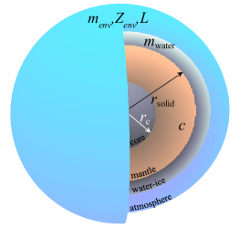
b) model II

Figure 1: Illustration of model parameterization. (a) Model I parameters are core radius $r_{\rm core}$, mantle composition $c$ comprising the oxides Na₂O–CaO–FeO–MgO–Al₂O₃–SiO₂, mantle radius $r_{\rm mantle}$, mass of water $m_{\rm water}$, mass of envelope $m_{\rm env}$, envelope Luminosity $L$, and envelope metallicity $Z_{\rm env}$. (b) Model II parameters are as for a), with atmosphere parameterized by pressure at the bottom of the atmosphere $p_{\rm batm}$, number of scale-heights of opaque layers $N$, mean molecular weight $\mu$, and a temperature-related parameter $\alpha$. See Section 2.2 and table 1 for more details.

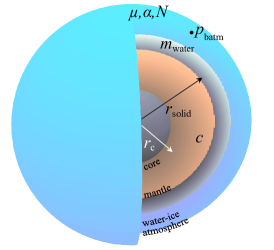
2.3 Data

The data d that we rely on are listed in Table 2.

Table 2: Summary of data d. We do not account for uncertainty in those parameters that are labeled as ‘fixed’.

parameter	description	comment
$M$	planetary mass
$R$	planetary radius
${\rm Fe}/{\rm Si}_{\rm bulk}$	bulk planetary ratio Fe/Si
${\rm Mg}/{\rm Si}_{\rm bulk}$	bulk planetary ratio Mg/Si
$c_{\rm minor}$	mantle composition of minor elements: CaO, Al2O3, Na2O	fixed
$a$	semi-major axis	fixed
$R_{\rm star}$	stellar radius	fixed
$T_{\rm star}$	stellar effective temperature	fixed

${\rm Fe}/{\rm Si}_{\rm bulk}$ is the mass ratio between the mass of iron to silicate for the entire planet (core and mantle), whereas ${\rm Fe}/{\rm Si}_{\rm mantle}$ is only that which is contained in the mantle. Since all magnesium and silicate are in the mantle, ${\rm Mg}/{\rm Si}_{\rm bulk}$ equals their mass ratio for the mantle ${\rm Mg}/{\rm Si}_{\rm mantle}$. We use the stellar abundances (${\rm Fe}/{\rm Si}_{\rm star}$ and ${\rm Mg}/{\rm Si}_{\rm star}$) as a proxy for ${\rm Fe}/{\rm Si}_{\rm bulk}$ and ${\rm Mg}/{\rm Si}_{\rm bulk}$. Similarly, we fix the absolute abundance of minor refractory elements (Na, Ca, and Al) in the mantle $c_{\rm minor}$ to stellar values. Here, we consider solar estimates for Fe/Si and Mg/Si and associated uncertainties, as well as Na₂O, CaO, and Al₂O₃ using the values of (Lodders et al., 2009). Stellar radius, and stellar effective temperature are also fixed parameters. Because uncertainty on stellar radius is generally small compared to uncertainties on planet radius, we neglect possible correlations between both and fix stellar radius.

2.4 Structure model

Data d and model parameters m are linked by a physical model embodied by the forward operator $g(\cdot)$.

$${\bf d}=g({\bf m})$$ (3)

For a given model ${\bf m}$ of the interior structure, mass $M$, radius $R$, and ${\rm Fe}/{\rm Si}_{\rm bulk}$ are computed and compared with observed data ${\bf d}$. The function $g({\bf m})$ combines thermodynamic, Equation-of-State (EoS), and atmospheric modeling as described in the following sections.

2.4.1 Iron core

In our model, we assume that the core is made of pure solid hcp (hexagonal close-packed) iron. Unlike in Earth’s core, we neglect light elements and nickel and disregard other iron polymorphs that stabilize at high temperatures. To compute the core density profile, we use an EoS for hcp iron provided by Bouchet et al. (2013). It is based on results obtained from ab initio molecular dynamics simulations for pressures up to 1500 GPa and temperatures up to about 15000 K and is in good agreement with experimental data obtained at Earth’s core conditions. This extensive pressure-temperature ($p$-$T$) range allows for modeling rocky exoplanets up to ten Earth masses (M). Throughout, we assume an adiabatic temperature profile.

2.4.2 Silicate mantle

Computing the mantle density profile is done in a manner analogous to Dorn et al. (2015). Equilibrium mineralogy and density are computed as a function of pressure, temperature, and bulk composition by Gibbs energy minimization (Connolly, 2009) within the model chemical system Na₂O-CaO-FeO-MgO-Al₂O₃-SiO₂. For these calculations the pressure is obtained by integrating the load from the surface boundary condition. As in Dorn et al. (2015) we fix the thermal gradient in the mantle based on the adiabatic gradient of Earth’s mantle. The mantle surface temperature equals the maximum of either the temperature at the bottom of the water layer or 1600 K (usual reference temperature of the Earth). For this purpose, we adopt the thermodynamic formulation of Stixrude & Lithgow-Bertelloni (2005) and parameters given in Stixrude & Lithgow-Bertelloni (2011).

2.4.3 Water layer

Water has a rich phase diagram with a variety of structural transitions depending on temperature and pressure (e.g., French et al., 2009). In most of our planet realizations, temperatures in the water layer generally range from $\sim$250 K to $\sim$1000 K and pressures up to a few hundred GPa. In order to compute the density profile of the water layer, we follow Vazan et al. (2013), using a quotidian equation of state (QEoS), which combines the Cowan ion EoS with the Thomas-Fermi model for electrons and treats H₂O as a mixture of atoms. This QEoS is in good agreement with the widely used ANEOS (Thompson & Lauson, 1972) and SESAME EoS (Lyon & Johnson, 1992). Above 44.3 GPa, we use the tabulated EoS from Seager et al. (2007) that is derived from DFT simulations and predict a gradual transformation from ice VIII to X. We assume an adiabatic thermal profile in the ice layer.

2.4.4 Atmospheric models

Previous works on mass-radius relationships are often restricted to pure H/He envelopes (e.g., Rogers & Seager, 2010; Howe et al., 2014). However, the compositional diversity might be large (Newsom, 1995) and significantly effect radius (e.g., Baraffe et al., 2008; Vazan et al., 2015). Here, we employ two different atmospheric models that account for enriched atmospheres (with the caveat of assuming ideal gas behavior). Model I solves the radiative transfer equation. This model assumes ideal gas behavior and accounts for the presence of H, He, C, and O. It considers opacities that are adapted to solar abundances (Lodders, 2003). More detailed and complex calculation of absorption and emission coefficients that inherit self-consistent opacities, scattering, clouds, and non-equilibrium chemistry could theoretically also be taken into account. However, in practice, the sparseness of available data does not warrant a more sophisticated treatment. Mass and radius observations will only allow us to constrain key characteristics of the envelope. For comparison, we also employ a second atmospheric model II that calculates an isothermal atmosphere with a simple pressure model using the scale-height model. Model II is computationally very inexpensive. The validity of models I and II is roughly restricted to 0.01 ¿ $m_{\rm env}$/$M$ and 0.0001 ¿ $m_{\rm env}$/$M$, respectively. Details on these limits are discussed in Section 3.2.2. Both models are described in the following.

Atmospheric model I

relies on the atmospheric code presented in Venturini et al. (2015), which has been adapted to compute planetary radii. For a radius and mass of the solid interior, distance to star $a$, stellar effective temperature $T_{\rm star}$, stellar radius $R_{\rm star}$, planet envelope luminosity $L$, envelope metallicity $Z_{\rm env}$, and envelope mass $m_{\rm env}$, we solve the equations of hydrostatic equilibrium, mass conservation, and energy transport. As in Venturini et al. (2015), we implement the CEA (Chemical Equilibrium with Applications) package (Gordon & McBride, 1994) for the EoS, which performs chemical equilibrium calculations for an arbitrary gaseous mixture, including dissociation and ionization and assuming ideal gas behavior. We assume an envelope with an elemental composition of H, He, C, and O. We define the envelope metallicity as the mass fraction of C and O in the envelope, which can vary between 0 and 1. The reason to implement CEA and not a more sophisticated EoS (for example, one that can take into account degeneracy of free electrons) is simply because no such EoS exists for an arbitrary mixture of H, He, C, and O.

These chemical elements are fundamental because they allow for the formation of key atmospheric molecules such as H₂O, CH₄, CO₂, and CO (Madhusudhan, 2012; Lodders, 2002; Visscher & Moses, 2011; Heng and Lyons, 2016). Moreover, effects of electron degeneracy pressure are important to compute radius of planets with massive envelopes. Even for the most extreme model realizations in this study where the mass fraction of the envelope is about 1 % (for a planet of 7 M), we expect the error to be less than 10 % in radius.

For the energy transport, we adopt the model presented in Jin et al. (2014), where an irradiated atmosphere is assumed at the top of the gaseous envelope and for which the analytic irradiation model of Guillot et al. (2010) is adopted. This irradiation model assumes a semi-gray, globally averaged temperature profile. Specifically we are using an analytical solution of the radiative transfer equation in the two-stream approximation. This irradiation model assumes a semi-gray, global temperature-averaged profile (Guillot et al., 2010), for which optical depth $\tau$ is related to the infrared mean opacity ($\kappa_{\text{th}}$) by $\nicefrac{{d\tau}}{{dr}}=\kappa_{\text{th}}\rho\,,$ where $\rho$ is density.

For the temperature gradient of the irradiated atmosphere, we solve the radial derivative of Eq. 49 of Guillot et al. (2010):

$$T^{4}= \frac{3T_{\text{int}}^{4}}{4}\bigg{[}\frac{2}{3}+\tau\bigg{]}+\frac{3T_{\text{eq}}^{4}}{4}\bigg{[}\frac{2}{3}+\frac{2}{3\gamma}\bigg{\{}1+\bigg{(}\frac{\gamma\tau}{2}-1\bigg{)}e^{-\gamma\tau}\bigg{\}}$$ (4)

$$+\frac{2\gamma}{3}\bigg{(}1-\frac{\tau^{2}}{2}\bigg{)}E_{2}(\gamma\tau)\bigg{]}\,,$$

where $\gamma=\kappa_{\text{v}}/\kappa_{\text{th}}$ is the ratio between visible and infrared opacity, $T_{\text{int}}$ is the intrinsic temperature given by $T_{\text{int}}=(L/(4\pi\sigma R_{P}^{2}))^{1/4}$, and $E_{2}(\gamma\tau)$ is the exponential integral, defined by $E_{n}(z)\equiv\int_{1}^{\infty}{t^{-n}e^{-zt}dt}$ with $n=2$. The boundary between the irradiated atmosphere and the envelope is set at $\gamma\tau=100/\sqrt{(}3)$ (Jin et al., 2014). For $\gamma\tau$ larger than this, the usual Schwarzschild criterion to distinguish between convective and radiative layers is applied. That is, if the adiabatic temperature gradient is larger than the radiative one, the layer is stable against convection, and the radiative diffusion approximation is used for computing the temperature gradient:

$$\frac{dT}{dr}=-\frac{3\kappa_{\text{th}}L\rho}{64\pi\bar{\sigma}T^{3}r^{2}}\,\,,$$ (5)

where $L$ is the intrinsic luminosity, $\bar{\sigma}$ is the Stefan-Boltzmann constant. Since we do not perform evolutionary calculations, $L$ is a model parameter (see Section 2.2). However, when the radiative gradient is larger than the adiabatic gradient, the layer is convective, and the temperature gradient is assumed to be adiabatic (which is computed with the EoS).

In Guillot et al. (2010), $\kappa_{\text{th}}$ and $\kappa_{\text{v}}$ (and therefore, $\gamma$) are free parameters. In order to reduce the number of free parameters, we use the prescription of Jin et al. (2014) who calibrate $\gamma$ for different equilibrium temperatures in order to reproduce results from more sophisticated atmospheric models for which a wavelength-dependent opacity function is used while solving for radiative equilibrium (Parmentier et al., 2013; Fortney et al., 2008). We implement this calibration in our numerical scheme, that is we interpolate the values of $\gamma$ for a given equilibrium temperature from Table 2 of Jin et al. (2014). In this way, without using detailed opacity calculations in the treatment of irradiation, we mimic the fundamental physics underlying atmospheric absorption and re-irradiation in a more simple (and numerically inexpensive) fashion. In order to compare the transit radius of a model realization with the measured radius from primary transits, we follow Guillot et al. (2010) and evaluate where the chord optical depth $\tau_{ch}$ becomes 2/3.

Atmospheric model II

assumes a simplified atmospheric model with a thin, isothermal atmosphere in hydrostatic equilibrium and ideal gas behavior, which is calculated using the scale-height model. For a given pressure $p_{\rm batm}$, mean molecular weight $\mu$, mean temperature (parameterized by $\alpha$), number of scale heights of opaque layers $N$ and a given solid interior we compute planet radius.

The scale-height $H$ is the increase in altitude for which the pressure drops by a factor of $e$ and can be expressed by

$$H=\frac{T_{\rm atm}R^{*}}{g_{\rm batm}\mu},$$ (6)

where $g_{\rm batm}$ and $T_{\rm atm}$ are gravity at the bottom of the atmosphere and atmospheric temperature, respectively. $R^{*}$ is the universal gas constant (8.3144598 J mol^-1 K^-1) and $\mu$ the mean molecular weight. The pressure $p$ at a given depth $z$ is the result of weight of the overlying gas layers. The hydrostatic equilibrium equation gives:

$$\frac{dp}{dz}=-gp.$$ (7)

With the assumption that gravity $g$ is constant and using the EoS for ideal gas, the density $\rho$ can be expressed as:

$$\rho=\frac{pR^{*}}{T_{\rm atm}\mu}.$$ (8)

The combination of the previous equations and the subsequent integration over pressure and altitude $z$ ($z=0$ where $p=p_{0}$ and $\rho=\rho_{0}$) leads to $p=p_{0}\exp(-\nicefrac{{z}}{{H}})$ and $\rho=\rho_{0}\exp(-\nicefrac{{z}}{{H}}).$

The mass of the atmosphere $m_{\rm atm}$ is directly related to the pressure $p_{\rm batm}$ as:

$$m_{\rm atm}=4\pi p_{\rm batm}\frac{r_{\rm batm}^{2}}{g_{\rm batm}}.$$ (9)

where $r_{\rm batm}$ and $p_{\rm batm}$ are radius and pressure at the bottom of the atmosphere, respectively. The thickness of the opaque atmosphere layer $z_{\rm atm}$ is:

$$z_{\rm atm}=HN,$$ (10)

where $N$ is the number of opaque scale-heights $H$. The atmosphere’s constant temperature is defined as

$$T_{\rm atm}=\alpha T_{\rm star}\sqrt{\frac{R_{\rm star}}{2a}},$$ (11)

where $R_{\rm star}$ and $T_{\rm star}$ are radius and effective temperature of the host star and $a$ is semi-major axes. The factor $\alpha$ is a model parameter (see Section 2.2) and incorporates possible cooling and heating of the atmosphere, it can vary between 0 and $\alpha_{\rm max}$. There is an upper bound $\alpha_{\rm max}$, because there is a physical limit to the amount of warming by greenhouse gases. We approximate $\alpha_{\rm max}$ for a moist (water-saturated) atmosphere (see Appendix A).

Generally, atmospheres can contain trace elements present at low pressures that have negligible contribution to the mass of the envelope but a significant contribution to the optical depth. In order to account for such effects, we use $p_{\rm batm}$ and $N$ as independent parameters.

We have chosen to make model II very general, that is we decouple structure and transmissivity of the gas layer by distinguishing between $\mu$ and $N$. The equivalent procedure of this in model I would be to define opacities as free parameters. Model II has four compared to three degree of freedom in model I.

Table 3: Prior model parameter ranges.

parameter	prior range	distribution	model
$r_{\rm core}$	0.01$r_{\rm solid}$ – 1 $r_{\rm solid}$	uniform in $r_{\rm core}^{3}$	I, II
${\rm Fe}/{\rm Si}_{\rm mantle}$	0 – ${\rm Fe}/{\rm Si}_{\rm star}$	uniform	I, II
${\rm Mg}/{\rm Si}_{\rm mantle}$	${\rm Mg}/{\rm Si}_{\rm star}$	Gaussian	I, II
$r_{\rm solid}$	0.01$R$ – 1.1 $R$	uniform	I, II
$m_{\rm water-ice}$	0 – 0.98 $M$	uniform	I, II
$m_{\rm env}$	$10^{-10}$ M – 0.9 $M$	uniform in log($m_{\rm env}$)	I
$L$	$10^{18}-10^{23}$ erg/s	uniform in log($L$)	I
$Z_{\rm env}$	0 – 1	uniform in 1/$Z_{\rm env}$	I
$p_{\rm batm}$	10-4 – 109 Pa	uniform in log($p_{\rm batm}$)	II
$N$	0 – log(109/10-4) $\approx$ 30	uniform	II
$\mu$	2.3 – 50.0	uniform in 1/$\mu$	II
$\alpha$	0.0 – $\alpha_{\rm max}$	uniform	II

2.5 Prior information

Table 3 lists prior parameter distributions. The chosen prior parameters distributions are wide reflecting a conservative choice. Different priors are discussed in Section 3.3.

Prior bounds on ${\rm Fe}/{\rm Si}_{\rm mantle}$ and ${\rm Mg}/{\rm Si}_{\rm mantle}$ are linked to the stellar abundance constraints. Since all Si and Mg are assumed to be in the mantle, ${\rm Mg}/{\rm Si}_{\rm star}$ defines the prior on ${\rm Mg}/{\rm Si}_{\rm mantle}$. We assume ${\rm Mg}/{\rm Si}_{\rm star}$ to be Gaussian distributed. Fe, on the other hand, is distributed between core and mantle. Thus, the bulk abundance constraint ${\rm Fe}/{\rm Si}_{\rm bulk}$ (= ${\rm Fe}/{\rm Si}_{\rm star}$) defines only the upper bound of the prior on ${\rm Fe}/{\rm Si}_{\rm mantle}$. There is an additional numerical limitation that the absolute iron oxide abundance in the mantle cannot exceed 70 %. For $p_{\rm batm}$ (model II), $m_{\rm env}$ and $L$ (model I), we assume the logarithm of these parameters to be uniformly distributed. The upper bound on the mass of the envelope in model I is set to 90 % of the planet mass, which is roughly the scale of Saturn and possibly Jupiter. The range of luminosities $L$ is chosen such that it embraces those of the Moon and Neptune. For model II, the mass of the envelope is parameterized through $p_{\rm batm}$. Its prior upper bound is arbitrarily set to 1 GPa. At such high pressures, the atmosphere may no longer behave like a gas and the simplified pressure scale-height model becomes invalid (e.g., Andrews, 2010). Only model realizations with $p_{\rm batm}$ well below 1 GPa can be used for further interpretation. The temperature-related parameter $\alpha$ uniformly varies between 0 and $\alpha_{\rm max}$, making up for possible cooling and heating of the atmosphere; $\alpha_{\rm max}$ scales with surface gravity (see Appendix A).

An example of the influence of different priors on interior model predictions is discussed at the end of this study. Some examples are also shown in Rogers & Seager (2010). In a future study, we will address this problem in more detail.

3 Results

Figure 2: Sampled one-dimensional (1-D) marginal posterior cdfs (blue) of model I parameters for Neptune: (a) mass of envelope $m_{\rm env}$, (b) envelope Luminosity $L$, (c) mass of water $m_{\rm water}$, (d) mantle radius $r_{\rm mantle}$, (e) core radius $r_{\rm core}$, (f) ${\rm Fe}/{\rm Si}_{\rm mantle}$, (g) ${\rm Mg}/{\rm Si}_{\rm mantle}$. Prior and posterior nearly completely overlap in (g). The envelope metallicity $Z_{\rm env}$ (not shown) is fixed, $Z_{\rm env}$ = 0. The prior cdfs are plotted in red. Gray area in plots (a-d) represent independent literature estimates (see main text).

Figure 3: Sampled two-dimensional (2-D) marginal posterior pdfs (blue) of model I parameters for Neptune: (a) mass of envelope $m_{\rm env}$ and envelope Luminosity $L$, (b) mass of water $m_{\rm water}$ and mantle radius $r_{\rm mantle}$. Gray areas represent independent literature estimates (see main text).

Figure 4: Sampled 1-D marginal posterior cdfs (blue) of model II parameters for Neptune: (a) pressure at bottom of atmosphere $p_{\rm batm}$, (b) atmospheric mass fraction m_atm/M (Eq. 9), (c) temperature-related parameter $\alpha$, (d) number of scale-heights of opaque layers $N$, (e) mean molecular weight $\mu$, (f) mass of water $m_{\rm water}$, (g) mantle radius $r_{\rm mantle}$, (h) core radius $r_{\rm core}$, (i) ${\rm Fe}/{\rm Si}_{\rm mantle}$, (j) ${\rm Mg}/{\rm Si}_{\rm mantle}$. The prior cdfs are plotted in red. Gray areas in (b,e,f) represent independent literature estimates (see main text).

3.1 Method validation: Neptune

As in Dorn et al. (2015), we validate the methodology against solar system planets. Here, we compare with Neptune ($M=$17.15 M, $R=3.87$ R, where R is 1 Earth radius), the smallest volatile-rich solar system planet. For model I, we have restricted the gas envelope to a pure H/He gas layer ($Z_{\rm env}$ = 0) and use the more appropriate EoS of Saumon et al. (1995) for Neptune, since the (otherwise employed) assumption of ideal gas behavior can result in radius uncertainties larger than 10 % for a gas mass fractions of a few percent. Although both atmospheric models I and II are not specifically tailored for Neptune, their application serve as a benchmark test and are not meant to provide new insights on Neptune’s interior.

For Neptune, geophysical data (gravitational and magnetic moments, solid-body rotation period, and heat flux) and atmospheric composition estimates are available that provide us with constraints on a possible three-component interior: (1) an outermost molecular envelope largely composed of H/He, (2) a weakly conducting ionic ocean of water, methane, and ammonia, and (3) a rocky central core (e.g., Soderlund et al., 2013; Podolak et al., 2000; Ness et al., 1989). The transition between outermost envelope and ocean is predicted to be around 0.8 $R$ by Lee et al. (2006), whereas the transition from ocean to rock likely occurs below 0.3 $R$ (Redmer, 2011). The transitions are neither well determined (Podolak et al., 2000; Nettelmann et al., 2013) nor necessarly sharp (Helled et al., 2010). For a three-component structure of H/He, H₂O, and SiO₂, Helled et al. (2010) suggest an upper bound on the water mass fraction of 90 % and an upper bound on the envelope mass fraction of 24 %. If the ice/rock ratio is restricted to proto-solar, Hubbard et al. (1995) find that Neptune could consist of about 25 % rock, 60-70 % ice, and 5-15 % gas by mass.

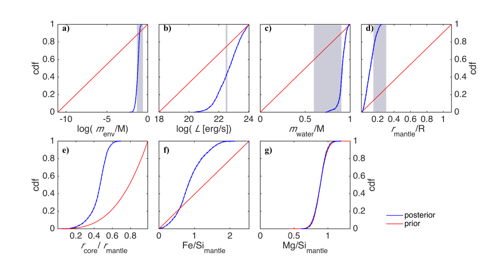
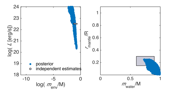
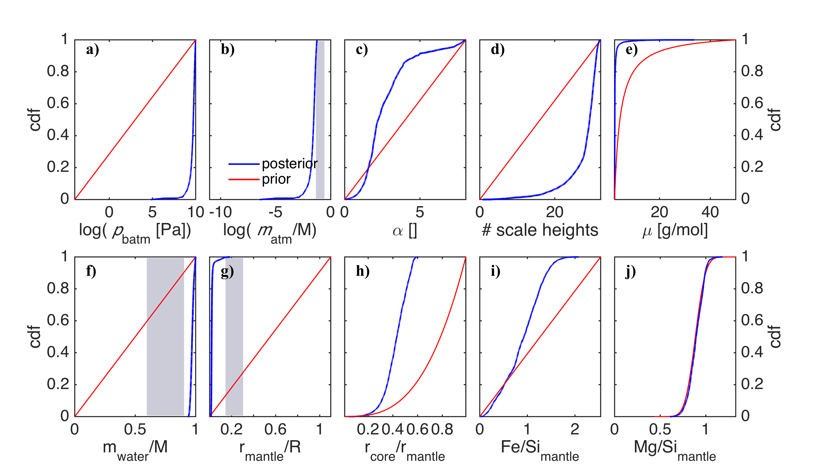
Here, we use uncertainties of $1\leavevmode\nobreak\ \%$ on both the observed $M$ and $R$, and $10\leavevmode\nobreak\ \%$ on the solar ratios ${\rm Fe}/{\rm Si}_{\rm star}$ and ${\rm Mg}/{\rm Si}_{\rm star}$ (Lodders, 2003). Results for the two atmospheric models are shown in Figures 2 and 4, respectively. The one-dimensional (1-D) marginal posterior cumulative distribution function (cdf) for each model parameter (in blue) is plotted with the prior distribution (in red) and independent parameter estimates (gray areas). The cdf describes the probability of a model parameter m with a certain probability distribution to be less or equal to a given value of m. In addition, Figure 3 shows the 2-D marginal posterior pdfs for those model parameters of model I for which we have independent estimates. These plots suggest the following:

• The interior structure of Neptune is constrained by the data.

• Available independent parameter estimates (shown in gray) overlap with the blue posterior cdfs for $m_{\rm env}$, $L$, $m_{\rm water}$, and $r_{\rm mantle}$ (model I, Figures 2 and 3); for model II (Figure 4) this is only the case for $m_{\rm atm}$ (derived from $p_{\rm batm}$ and Eq. 9), $m_{\rm water}$ and $r_{\rm mantle}$ are over-and under-predicted, respectively.

• With only mass, radius, and abundance constraints, our method (model I) predicts independent geophysical estimates of Neptune’s interior. Compared to independent estimates, our calculated confidence regions for the structural parameters are larger, since we rely on limited data:

  • 0.01 $<$ $m_{\rm env}$/$M$ $<$ 0.2,

  • 0.75 $<$ $m_{\rm water}$/$M$ $<$ 0.98,

  • 0.01$<$ $r_{\rm mantle}$ $<$ 0.25,

  • $10^{21}$ erg/s$<L<10^{24}$ erg/s.

• The simplified pressure model II leads to an overestimation of $m_{\rm water}$ and underestimation of $r_{\rm mantle}$ compared to model I. This is because the same radius fraction of gas results in different $p$-$T$ boundary conditions for the ice layer for both models. The simplified pressure model II generally overestimates $p_{\rm batm}$, which leads to an increase in water ice density. In order to fit the radius, the higher water ice density implies a larger $m_{\rm water}$. At the same time, the mass contribution of the rocks needs to be reduced so as not to overestimate mass.

Without the restriction to pure H/He in model I and under the assumption of ideal gas, the results are similar with the largest discrepancy in the estimate of a gas mass fraction (with a 50%-percentile of 0.01 $m_{\rm env}$/M under the ideal gas premise compared to 0.06 $m_{\rm env}$/$M$ in Figure 2).

Table 4: Data of synthetic planets.

name	$M$ [M ]	$\sigma_{M}$	$R$ [R ]	$\sigma_{R}$	$\sigma_{{\rm Fe}/{\rm Si}_{\rm bulk}}$	$\sigma_{{\rm Mg}/{\rm Si}_{\rm bulk}}$	semi-major axis [AU]	$\bar{\rho}$ [g/cm3]	additional comments
Case A	7	5 %	1.7	2 %	20 %	20 %	1	7.86	Figs. 6, 7
Case B	7	5 %	2.2	2 %	20 %	20 %	1	3.62	Figs. 6, 7, 11, 10
Case C	7	5 %	2.6	2 %	20 %	20 %	1	2.20	Figs. 6, 7, 12, 8, 9
Case D	7	5 %	2.9	2 %	20 %	20 %	1	1.58	Figs. 6, 7
Case E	7	20 %	2.2	10 %	20 %	20 %	1	3.62	Figs. 11, 10
Case F	7	5 %	2.2	2 %	50 %	50 %	1	3.62	Figs. 11, 10
Case G	7	5 %	2.2	2 %	80 %	80 %	1	3.62	Figs. 11, 10
Case H	7	5 %	2.6	2 %	20 %	20 %	0.1	2.20	Fig. 12
Case J	7	5 %	2.6	2 %	20 %	20 %	0.1	2.20	H/He atmosphere only, Fig. 12
Case K	7	5 %	2.6	2 %	20 %	20 %	1	2.20	H/He atmosphere only, Fig. 12

Figure 5: Masses and radii of synthetic planets (black dots, cases A-K), observed exoplanets (gray dots) from Dressing et al. (2015), and Earth and Venus. Planets are plotted against mass-radius curves of idealized compositions for which a surface temperature of 300 K has been assumed. Planet cases A-K are summarized in Table 4.

3.2 Synthetic cases

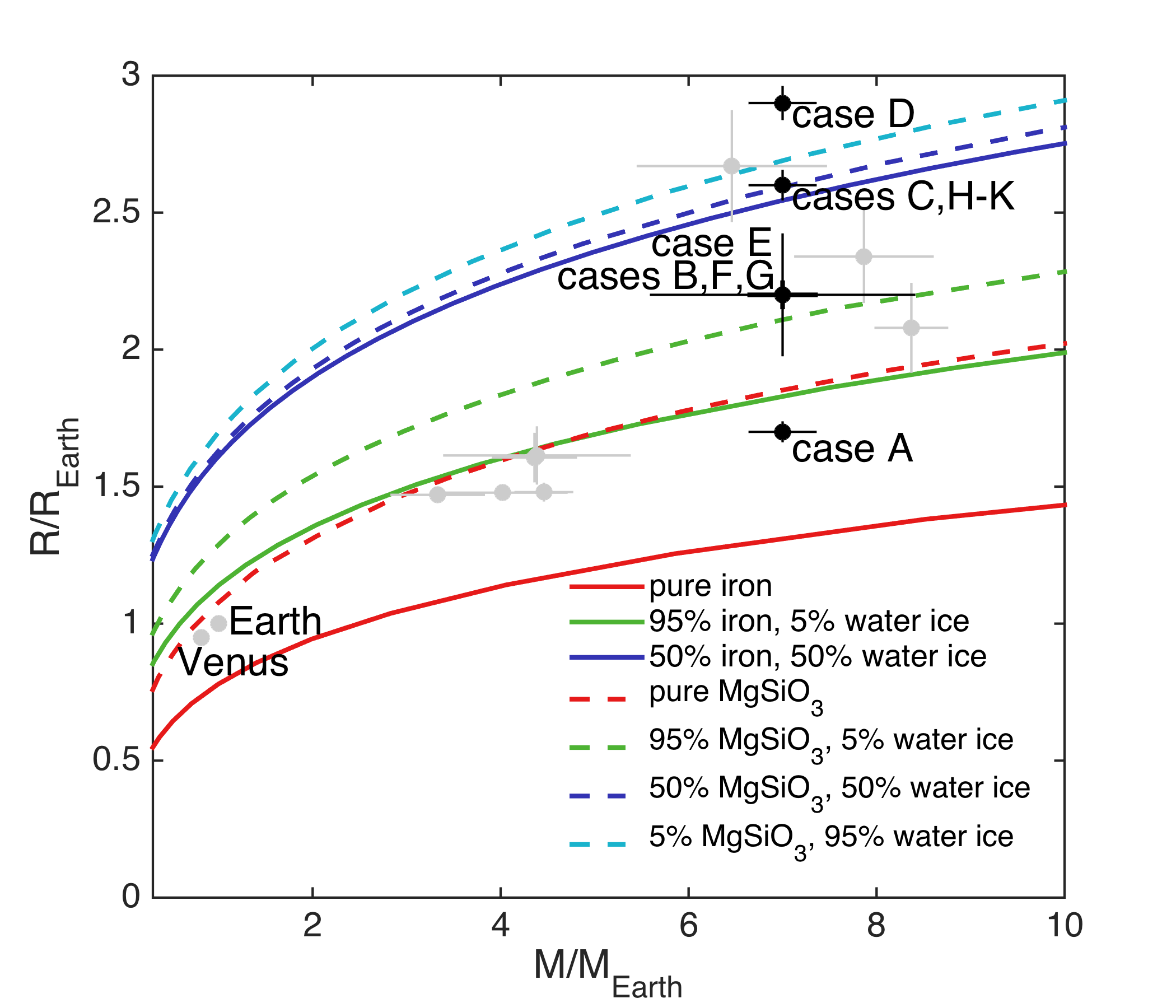
Next, we apply our method to synthetic exoplanets. Application to actual observations is presented in a companion paper (Dorn et al., 2017). In this study, we emphasize instead the influence of the following parameters on interior predicitions: bulk density $\bar{\rho}$, data uncertainties, semi-major axis, atmospheric composition, and prior distributions. For the latter, we test the a priori assumption of enriched envelopes versus pure H/He envelopes. For all synthetic planets we assume $M=7$ M, since the transition between rocky and non-rocky planets seems to occurr around this mass (e.g., Weiss & Marcy, 2014; Rogers, 2015). Table 4 lists all relevant data for the synthetic cases and Figure 5 shows their masses and radii plotted against curves of idealized compositions. For all synthetic cases, we assume solar values for abundance constraints (Lodders, 2003), stellar effective temperature and stellar radius of the Sun. In the following, we discuss these test cases.

Figure 6: Sampled 1-D marginal posterior cdfs of model I parameters for synthetic planet cases (A-D) of 7 M that vary in terms of radii: 1.7 R (A), 2.2 R (B), 2.6 R (C), 2.9 R (D); (a) mass of envelope $m_{\rm env}$, (b) envelope luminosity $L$, (c) envelope metallicity $Z_{\rm env}$, (d) mass of water $m_{\rm water}$, (e) mantle radius $r_{\rm mantle}$, (f) core radius $r_{\rm core}$, (g) ${\rm Fe}/{\rm Si}_{\rm mantle}$, (h) ${\rm Mg}/{\rm Si}_{\rm mantle}$.

Figure 7: Sampled 1-D marginal posterior cdfs of model II parameters for synthetic planet cases (A-D) of 7 M that vary in terms of radii: 1.7 R (A), 2.2 R (B), 2.6 R (C), 2.9 R (D); (a) pressure at bottom of atmosphere $p_{\rm batm}$, (b) atmospheric mean molecular weight $\mu$, (c) temperature-related parameter $\alpha$, (d) number of scale-heights of opaque layers $N$, (e) mass of water $m_{\rm water}$, (f) mantle radius $r_{\rm mantle}$, (g) core radius $r_{\rm core}$, (h) ${\rm Fe}/{\rm Si}_{\rm mantle}$, (i) ${\rm Mg}/{\rm Si}_{\rm mantle}$. Depending on the case, the upper prior bound in (c) differs, which is indicated by the vertical colored lines corresponding to the respective case.

3.2.1 Influence of bulk density

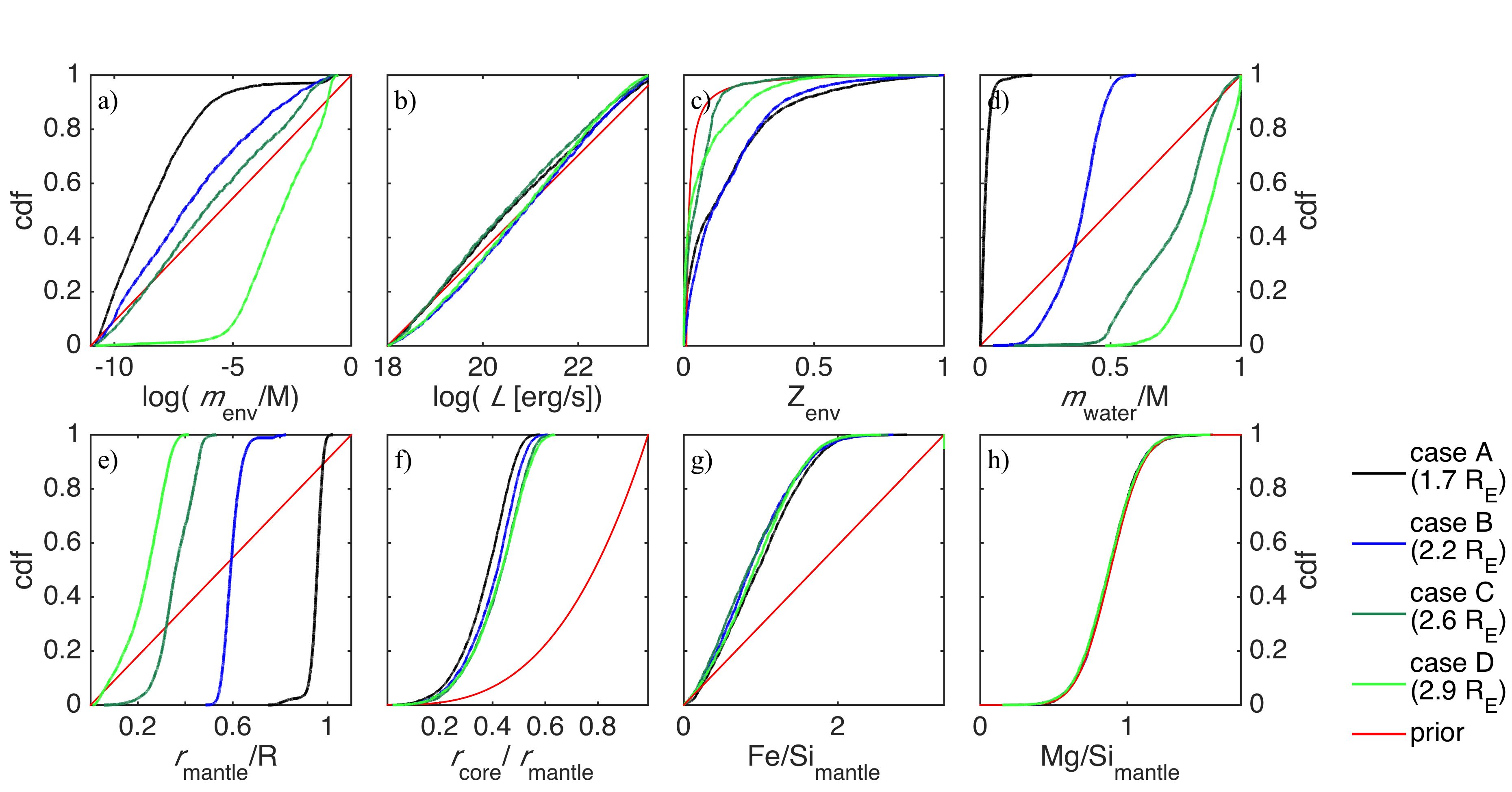
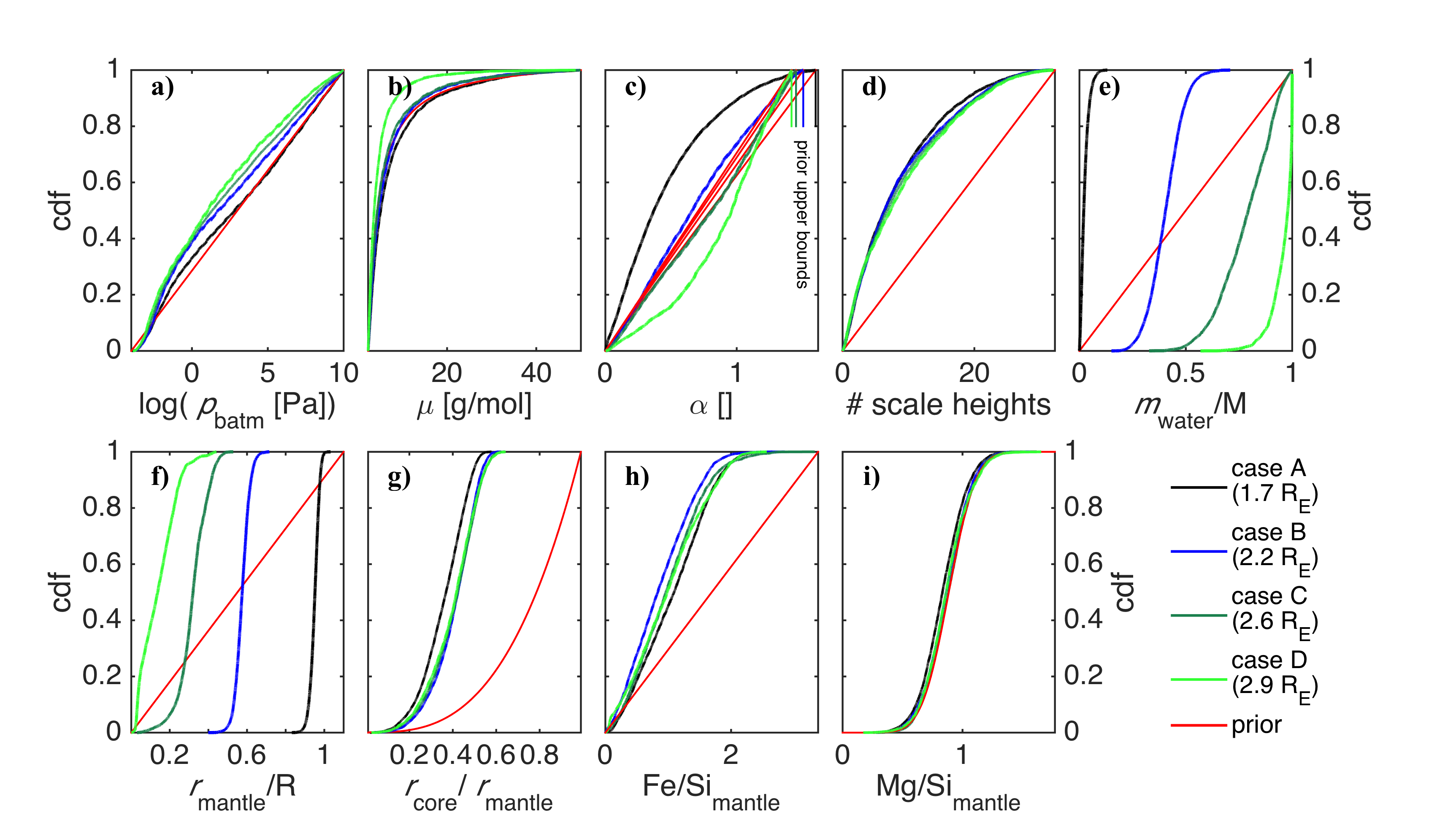
Planets A, B, C, and D are assigned different radii (1.7, 2.2, 2.6, and 2.9 R) and hence bulk densities $\bar{\rho}$ (Table 4). Uncertainties for mass and radius are assumed to be similar to the predicted uncertainties from the PLATO mission (Rauer et al., 2014), that is 5% and 2%, respectively. The influence of planet bulk density on retrieved parameters is shown in Figures 6 and 7. We observe, as expected, that bulk density correlates positively with the size of the rocky interior $r_{\rm mantle}$, and correlates negatively with mass of water ($m_{\rm water}$) and gas ($m_{\rm env}$). Core size and mantle composition (Figure 6f-h and 7g-i) show only small variations, because they are constrained by the solar abundances.

Among the parameters characterizing the gas layer for model I (Figure 6), $m_{\rm env}$ and $Z_{\rm env}$ are constrained by data, whereas envelope luminosity $L$ is not. For the planet with the highest bulk density (case A) the gas layer contributes very little to planet radius, i.e., metallicity is high and/or $m_{\rm env}$ is small. Case A is found with a 90 % probability to have an atmosphere smaller in mass than Earth ($10^{-7}$ $m_{\rm env}$/$M$). Compared to high bulk density planets, low density planets can have gas of lower metallicity while gas mass fraction tends to be higher. For very low density planets (case D) when even pure water ice is not sufficient to explain radius, small $m_{\rm env}$ are excluded as a result of which $m_{\rm env}$ is larger than $10^{-5}$ $M$ with a probability of 90 %.

The gas layer parameters for model II (Figure 7) indicate that the number of opaque scale-heights $N$ and temperature (parameterized by $\alpha$) in the gas layer appear to be best constrained by data. The expected trend of a higher temperature (larger $\alpha$) and an increased number of scale-heights that are needed to explain low bulk density planets is clearly visible (Figure 7c and d). Mean molecular weight $\mu$ and $p_{\rm batm}$ are both weakly constrained for the high bulk density cases (A, B, and C). When pure water ice cannot compensate enough to fit radius (case D compared to the other cases) the gas layer moves to higher pressures $p_{\rm batm}$, lower mean molecular weights, higher temperatures ($\alpha$), and more scale-heights (Figure 7 light green curve).

Although the use of both atmospheric models yield very similar parameter distributions for the rocky part of the planet, there are significant differences in $m_{\rm water}$, particulary for the low density planets (cases C and D). This is because parameters related to gas and ice layers are those with the largest influence on planet radius. Hence differences in the atmospheric model affect the gas structure and in consequence the distribution of $m_{\rm water}$. We will discuss these differences in more detail in the following.

Figure 8: Sampled 2-D marginal posterior pdfs of model I parameters for synthetic planet case C showing the correlation between: (a) $r_{\rm core}$ and $r_{\rm mantle}$, (b) $r_{\rm mantle}$ and $m_{\rm water}$, (c) $m_{\rm water}$ and $m_{\rm env}$, (d) $m_{\rm env}$, and $Z_{\rm env}$, (e) $m_{\rm water}$ and the averaged $\mu$ corresponding to $Z_{\rm env}$. Those model realizations that explain the data within 1-$\sigma$ are plotted in blue. Samples in (c, d) for which gas mass fractions $m_{\rm env}$/$M$ ¿ 0.01 are highlighted in green and should be taken with care. See main text for discussion of features B1 and B2.

Figure 9: Sampled 2-D marginal posterior pdfs of model II parameters for synthetic planet case C showing the correlation between: (a) $r_{\rm core}$ and $r_{\rm mantle}$, (b) $r_{\rm mantle}$ and $m_{\rm water}$, (c) $m_{\rm water}$ and $p_{\rm batm}$, (d) $p_{\rm batm}$, and $\mu$, (e) $m_{\rm water}$ and $\mu$, (f) $m_{\rm water}$ and $\alpha$, (g) $m_{\rm water}$ and $N$. Those model realizations that explain the data within 1-$\sigma$ are plotted in blue. Samples in (c, d) for which gas mass fractions $m_{\rm env}$/$M$ ¿ 0.0001 are highlighted in green and should be taken with care.

3.2.2 Influence of atmospheric model

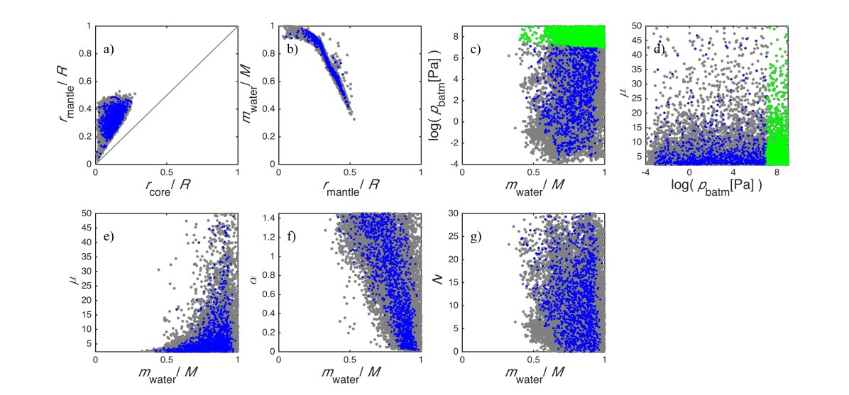
Here, we take a closer look at the different parameter estimates for case C when using model I and II. We plot the sampled 2-D marginal posterior distributions of model parameters in Figures 8 and 9. Overall, the distributions show similar trends with clear differences for the rocky and icy interior depending on atmospheric model:

• There is a strong correlation between $m_{\rm water}$ and $m_{\rm env}$ in model I (Figure 8). For model II, the corresponding correlation between $m_{\rm water}$ and $p_{\rm batm}$ is weak. This reflects a higher degeneracy in the gas layer parameters for model II (more degrees of freedom).

• For model II, strongest correlations with $m_{\rm water}$ are seen for $\mu$ and $\alpha$ among the gas parameters.

• For model I compared to model II, $r_{\rm mantle}$ tends to be larger (Figures 8a and 9a).

• There is a clear discrepancy in the estimated $m_{\rm water}$ between the two models. For model I, the minimum $m_{\rm water}$ is estimated to be about 0.1 $M$, whereas for model II it is 0.5 $M$.

Model II leads to the misinterpretation that relatively low-density planets (case C) require a massive ocean to explain mass and radius. This is in line with earlier conclusions suggesting that it is impossible to distinguish between a thick atmosphere and an ocean based on mass and radius alone (e.g., Adams et al., 2008). This is important in view of the different formation histories implied by either interpretation. The results show that the simplified pressure model II fails to explain thicker atmospheres and thereby overestimates the amount of water ice. This is because it does not account for energy transport and thus overestimates the pressure increase with atmospheric depth. Thicker atmospheres can in principle be realized, if temperatures (i.e., $\alpha$) exceeding the prior range ($\alpha_{max}$, Appendix A) would be allowed, implying a larger greenhouse effect. However, there is a physical upper limit, the Komabayashi–Ingersoll Limit (Komabayasi, 1967; Ingersoll, 1969), to the amount of outgoing long-wave radiation that can be absorbed and emitted by greenhouse gases that warm the atmosphere. More advanced modeling would be required to determine this upper limit for the studied cases, but this is outside of the scope of this study.

In the 2-D plots (Figure 8b and c) showing the correlation between $r_{\rm mantle}$ and $r_{\rm core}$, and $r_{\rm mantle}$ and $m_{\rm water}$, respectively, two ‘branches’ (labeled B1 and B2) are visible (valid for massive atmospheres $m_{\rm env}$ $>$ 0.01 $M$ ) which are characterized by:

• B1:
  $m_{\rm water}$ $<$ 0.5 $M$,
  $Z_{\rm env}$ $<$ 0.02,
  $L>10^{22.5}$ erg/s

• B2:
  $m_{\rm water}$ $>$ 0.5 $M$,
  0.02 $<$$Z_{\rm env}$ $<$ 1.0,
  $10^{18}$erg/s $<L<10^{22.5}$ erg/s

For gas envelopes of supersolar abundances (B2), self-gravity of massive gas layers leads to compressed envelopes. To fit radius in this case, a large $m_{\rm water}$ is required. For subsolar abundances and very high luminosities (B1), the envelopes are thick and make up for a large fraction of planet radius (¿ 25%). However, a minimum $m_{\rm water}$ of 0.1 $M$ appears to be required to fit radius. This is because we restrict the prior range on luminosity $L$ to a maximum of $10^{23}$ erg/s (Neptune-like $10^{22.52}$ erg/s). If larger luminosities than the prior range were allowed, thicker gas layers with negligible ice mass fractions could be realized. This suggests that constraints on the luminosities would allow to partly lift the degeneracy between an ocean and a thick atmosphere. This will be investigated in more detail in the future.

We compare the planetary radii that are computed with both atmospheric models by using the calculated pressures and temperatures from model I (e.g., pressures at bottom and top of the gas layer and an averaged temperature) as input in model II for a rocky interior of 7 M. For an envelope mass of $m_{\rm env}$ $>10^{-3}$ M (corresponding to $p_{\rm batm}$ $\approx$ 1000 bar), the discrepancy in radius becomes comparable to the observed radius uncertainty of 2 %. We note that the comparison of both models is sensitive to the choice of temperature averaging. Hence, for large bulk density planets with thin atmospheres (cases A and B), the choice of atmospheric model does not significantly affect estimates of the rocky and icy interior (Figures 6 and 7), whereas it becomes relevant for relatively low-density planets (cases C and D).

For the cases studied here, we conclude that the more accurate representation of gas layer physics makes model I more favorable inspite of larger computational costs. In the case of thin atmospheres, model II is valid.

Figure 10: Sampled 1-D marginal posterior cdfs of model I parameters for synthetic planet cases B, E, F, G that vary in terms of data uncertainties. B is the reference case ($\sigma_{M}$=0.05 $M$, $\sigma_{R}$ = 0.02 $R$, 20 % for both $\sigma_{{\rm Fe}/{\rm Si}_{\rm bulk}}$ and $\sigma_{{\rm Mg}/{\rm Si}_{\rm bulk}}$), E has larger uncertainties in mass and radius ($\sigma_{M}$=0.2 $M$, $\sigma_{R}$ = 0.1 $R$), whereas F and G have larger uncertainties in the abundance constraints, 50 % and 80 %, respectively. (a) Mass of envelope $m_{\rm env}$, (b) envelope luminosity $L$, (c) envelope metallicity $Z_{\rm env}$, (d) mass of water $m_{\rm water}$, (e) mantle radius $r_{\rm mantle}$, (f) core radius $r_{\rm core}$, (g) ${\rm Fe}/{\rm Si}_{\rm mantle}$, (h) ${\rm Mg}/{\rm Si}_{\rm mantle}$. The priors in (g) and (h) are not shown as not to overload the plot, because they differ among the cases.

Figure 11: Sampled 1-D marginal posterior cdfs of model II parameters for synthetic planet cases B, E, F, G that vary in terms of data uncertainties. B is the reference case ($\sigma_{M}$=0.05 M, $\sigma_{R}$ = 0.02 $R$, 20 % for both $\sigma_{{\rm Fe}/{\rm Si}_{\rm bulk}}$ and $\sigma_{{\rm Mg}/{\rm Si}_{\rm bulk}}$), E has larger uncertainties in mass and radius ($\sigma_{M}$=0.2 $M$, $\sigma_{R}$ = 0.1 $R$), whereas F and G have larger uncertainties in the abundance constraints, 50 % and 80 %, respectively. (a) Pressure at bottom of atmosphere $p_{\rm batm}$, (b) atmospheric mean molecular weight $\mu$, (c) temperature-related parameter $\alpha$, (d) number of scale-heights of opaque layers $N$, (e) mass of water $m_{\rm water}$, (f) mantle radius $r_{\rm mantle}$, (g) core radius $r_{\rm core}$, (h) ${\rm Fe}/{\rm Si}_{\rm mantle}$, (i) ${\rm Mg}/{\rm Si}_{\rm mantle}$. The priors in (h) and (i) are not shown as not to overload the plot, because they differ among the cases.

3.2.3 Influence of data uncertainty

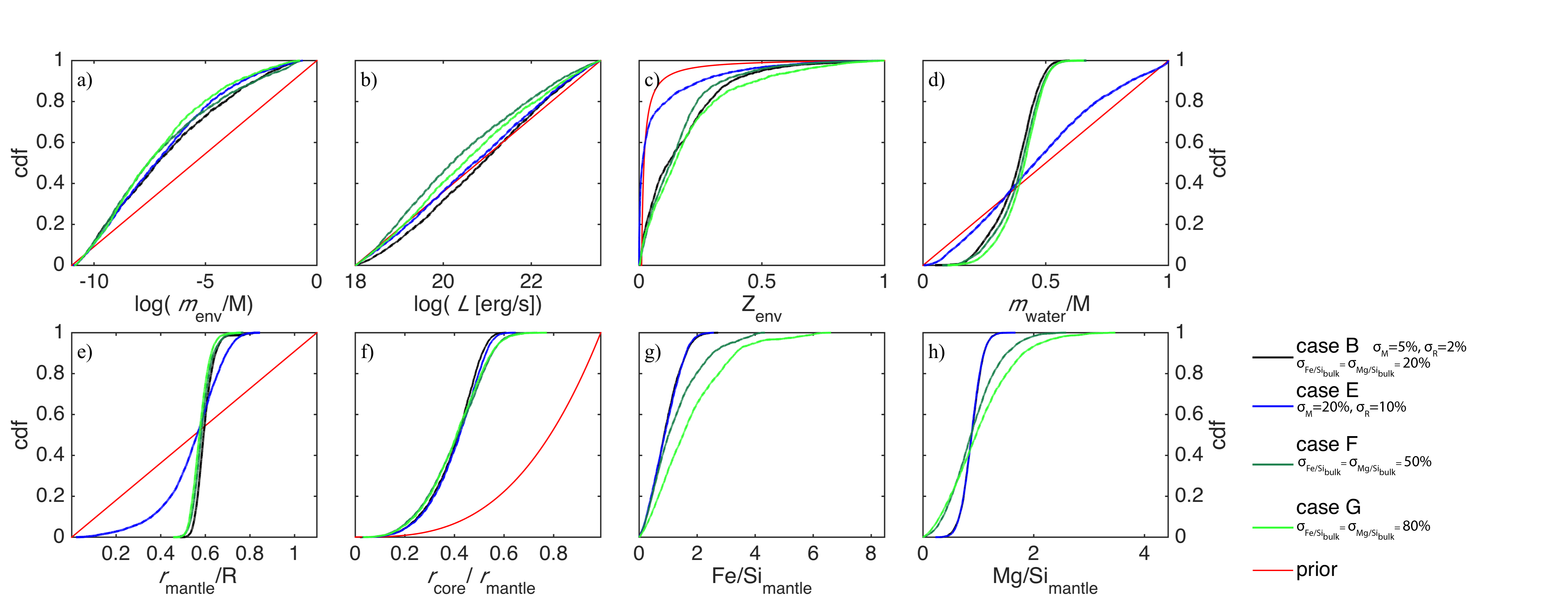
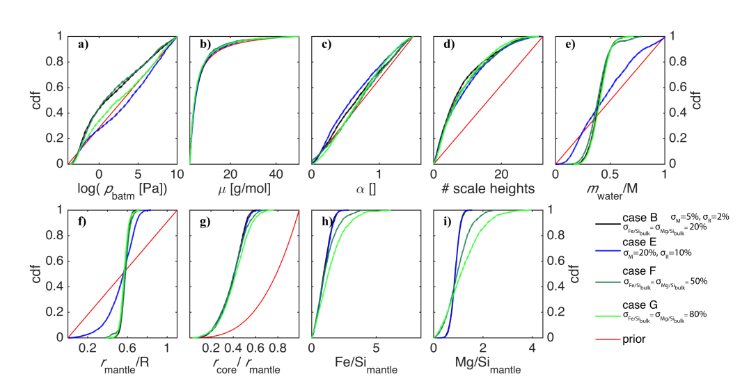
Here, we study the influence of data uncertainty on structural parameter estimation. As summarized in Table 4, we vary uncertainty in mass and radius between cases B ($\sigma_{M}$ of 5%, $\sigma_{R}$ of 2 %) and E ($\sigma_{M}$ of 20 %, $\sigma_{R}$ of 10 %); we vary uncertainties on planet bulk abundances between cases B (20 %), F (50 %), and G (80 %). All cases B, E, F, and G have the same bulk density of 3.62 g/cm³. The smallest chosen data uncertainties reflect those of high quality data similar to those expected from PLATO. Results are shown in Figures 10 and 11. The results can be summarized as follows:

• Mass and radius uncertainties mainly affect estimates of $r_{\rm mantle}$, $m_{\rm water}$, and $Z_{\rm env}$. For example, the retrieved confidence region for $r_{\rm mantle}$ and $m_{\rm water}$ is three times larger in case E compared to case B (the 5 % to 95 % percentile range of $r_{\rm mantle}$ for case E is 0.28–0.73 $R$ compared to 0.54–0.66 $R$ in case B; similarly the range of $m_{\rm water}$ for case E is 0.08–0.93 $M$ compared to 0.22–0.5 $M$ in case B).

• Mass and radius uncertainties do not significantly affect estimates of core and mantle composition, since they are conditioned to the same abundance constraints (cf. case B and E).

• Reducing the uncertainties on the abundance constraints mainly improves the ability to constrain the mantle composition. For example, the 5 % to 95 % percentile ranges for ${\rm Mg}/{\rm Si}_{\rm mantle}$ in cases F and G are larger by a factor of 2.6 and 3.4 compared to case B, respectively.

• Compared to the studied cases, the influence on determining core size is more pronounced for purely rocky planets as described by Dorn et al. (2015). Here, only moderate effects are seen for core size estimates, where the 5 % to 95 % percentile range of core size $r_{\rm core}$ is 30 % larger for case G compared to B.

• Uncertainties on the abundance constraints have only minor effects on estimates of $r_{\rm mantle}$ and $m_{\rm water}$. Between cases B and G, for example, the 50th percentile of $m_{\rm water}$ varies by up to 8 %.

For the studied cases, mass and radius uncertainties are more important than uncertainties on ${\rm Fe}/{\rm Si}_{\rm bulk}$ and ${\rm Mg}/{\rm Si}_{\rm bulk}$ to constrain key structural parameters such as $m_{\rm water}$ and $r_{\rm mantle}$. This conclusion might vary depending on the actual planet mass and bulk density.

Figure 12: Sampled 1-D marginal posterior cdfs of $m_{\rm env}$ (model I) for the synthetic planets: case C at 1 AU, case H at 0.1 AU, case J at 1 AU, and case K at 0.1 AU. For cases J and K, the gas composition is restricted to pure H/He ($Z_{\rm env}$ = 0) using the EoS of Saumon et al. (1995).

3.2.4 Influence of semi-major axes

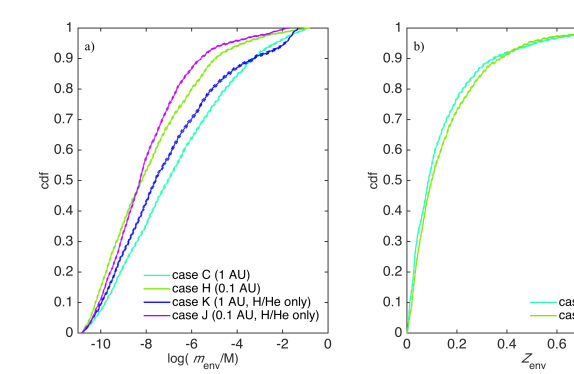
The semi-major axis influences the energy budget available in the gas envelope and thereby the radius of the planet. Figure 12 demonstrates the effect of distance to the star on estimates of $m_{\rm env}$. For the same planet with a smaller semi-major axis (case H compared to C), the interior can be explained by a smaller $m_{\rm env}$ and higher envelope metallicity $Z_{\rm env}$, although the effect on $Z_{\rm env}$ is small (not shown). This result is intuitive, since a hotter gas envelope implies a lower gas density, which results in a larger radius. Thus, in order to compensate for a higher intrinsic luminosity while still fitting the radius, the gas mass must be smaller and/or more heavier elements need to be present. If only pure H/He gas layers are considered, the same trend for $m_{\rm env}$ is observed (cases K and J in Figure 12a). Compared to metal-rich envelopes, the restriction to pure H/He envelopes leads to smaller $m_{\rm env}$ for the reason just discussed.

3.3 Influence of prior distribution

The results obtained by a Bayesian inference analysis are subject to the choice of prior, which, if not chosen carefully can lead to a significant imprint on parameters that are weakly constrained by data. In the following, we consider a number of different priors to illustrate this on a selected set of parameters that are sensed differently by the data considered here. We have singled out core size, which is largely determined by bulk abundances and mass, in addition to envelope metallicity and luminosity that are mainly constrained by radius and stellar irradiation.

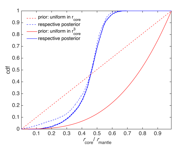
Figure 13 illustrates the effect of different prior choices on estimated (posterior) core size $r_{\rm core}$ for a Neptune-sized planet. Here, we contrast a uniform prior in $r_{\rm core}$ with a uniform prior in $r_{\rm core}$ ³. A uniform prior in $r_{\rm core}$ gives more weight to smaller core sizes relative to a uniform prior in $r_{\rm core}$ ³. But since $r_{\rm core}$ ³ is directly proportional to core mass it represents the more natural choice. The results indicate that the effect of the prior is negligible for the 50 %-percentile of $r_{\rm core}$. This is an example where the choice of prior is less significant.

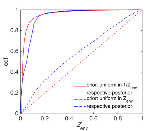
Next, we investigate an example where the estimated parameter is only weakly constrained by data. This is, for example, the case for envelope metallicity $Z_{\rm env}$. We compare a uniform prior in $Z_{\rm env}$ and in 1/$Z_{\rm env}$ for a case-C planet. A uniform prior in 1/$Z_{\rm env}$ is motivated by the fact that H and He are most abundant elements and that primary atmospheres are likely rich in H and He (e.g., Alibert et al., 2004). Also, the scale height of the gas layer correlates positively with 1/$Z_{\rm env}$. The results are shown in Figure 14 and illustrate that a uniform distribution in $Z_{\rm env}$, relative to a uniform in 1/$Z_{\rm env}$, gives more weight to larger envelope metallicities. This implies that we are favoring lighter-element atmospheres over heavier-elements. A uniform prior in $Z_{\rm env}$ may be more appropriate for secondary (outgassed) atmospheres, for which heavy element enrichment is a priori a more likely scenario.

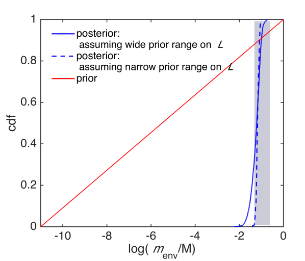
Finally, we consider luminosity $L$. For purposes of illustration, we chose the following range $10^{22.52\pm 0.05}$ erg/s, which corresponds to the observed luminosity of Neptune. More generally, additional constraints such as infrared flux measurements would allow for a narrower prior range on luminosity. Figure 15 illustrates the effect of assuming different prior ranges on $L$ in estimating gas mass fraction $m_{\rm env}$/M for the case of a Neptune-sized planet. The new prior range on $L$ leads to an improved constraint on gas mass fraction of 0.05$<$$m_{\rm env}$/$M<$0.09 that better predicts independent geophysical estimates relative to the earlier determined range (0.01$<$$m_{\rm env}$/$M<$0.2), where a relative wide prior range was invoked (Table 3). In this example, the choice of prior has no significant effect on the 50 %-percentile of $m_{\rm env}$/M.

From the above, we can conclude that the posterior distribution is mostly affected by the assumed prior distribution for those parameters that are weakly constrained by data. In summary, it should be emphasized that the choice of prior is not arbitrary but need to be based (whenever possible) on observations, laboratory measurements and/or theoretical considerations.

Figure 13: Sampled 1-D marginal posterior cdfs (blue) for different priors (red) of core size $r_{\rm core}$ for Neptune (applying model I). Distributions are depicted in dashed when the prior is uniform in $r_{\rm core}$ and solid when it is uniform in $r_{\rm core}$ ³. The latter is identical to Figure 2e.)

Figure 14: Sampled 1-D marginal posterior cdfs (blue) for different priors (red) of envelope metallicity $Z_{\rm env}$ for case C (7M, 2.6 R, applying model I). Distributions are depicted in dashed when the prior is uniform in $Z_{\rm env}$ and solid when it is uniform in 1/$Z_{\rm env}$. The latter is identical to Figure 6c.)

Figure 15: Sampled 1-D marginal posterior cdfs (blue) for $m_{\rm water}$ assuming different priors on $L$ for Neptune (applying model I). Solid blue line refer to wide prior range on $L$ ($10^{18}-10^{23}$ erg/s), whereas dashed blue line refer to narrow prior range on $L$ ($10^{22.47}-10^{22.57}$ erg/s). The former is identical to Figure 2a. Gray area represent independent literature estimates (see main text).

4 Discussion

Here, we have extended the method of Dorn et al. (2015) from purely rocky exoplanets to general exoplanet types that include volatile-rich layers in the form of water ice, oceans, and atmospheres. For the same data of mass, radius, and bulk abundance constraints, the degeneracy of core and mantle parameters is generally larger in planets of general structure than for purely rocky planets, since their contribution to mass and radius can in part be compensated by volatile material.

The key to constrain the structural parameters resides in the large density contrasts between rock, water, and gaseous layers. In other words, our ability to constrain interiors is because of the different data sensitivity of the various parameters. The abundance constraints couple core size with mantle size and composition. The relative sizes of core and mantle are thus determined by ${\rm Fe}/{\rm Si}_{\rm bulk}$. The mass of the planet mainly dictates the absolute size of the rocky part and the mass of water. Planetary radius meanwhile determines the characteristics of the envelope and the water layer.

The strength of the presented inference method is that it is modular, i.e., different interior structure models can be tested against each other. However, the applicability and informative value of the inference method is subject to imposed assumptions on the structure model. For example, the two tested atmospheric models differ in terms of complexity and general applicability.

Model I is more elaborate in that it calculates pressure-temperature profiles for a given composition while solving for hydrostatic equilibrium, mass conservation, and energy transport. But it is restricted to H, He, C, and O and it assumes equilibrium chemistry, ideal gas behavior, as well as prescribed opacities. The latter are fit to results of radiative equilibrium models that use a wavelength-dependent opacity function by Jin et al. (2014) for solar metallicities. In that regard, the opacities used are not self-consistent when non-solar metallicities are considered ($Z_{\rm env}$ $\neq$ 0.02). Different values of opacities can lead to differences in radius by up to 5 %. Models that compute line-by-line opacities with their corresponding atmospheric abundances should be performed in the future to compute planetary radii in a self-consistent way. The assumption of ideal gas behavior introduces a bias in radius for large atmospheric mass fractions, for example for a 1 % $m_{\rm env}$/$M$ planet atmosphere the difference in the radius between ideal gas and the Saumon et al. (1995) EoS (for H-He) can reach 10 %.

Model II assumes an isothermal, homogeneous atmosphere and ideal gas behavior. Therefore, model II is strictly only valid in the case of thin atmospheres ($m_{\rm env}$ $\lesssim 10^{-3}$ M). While, future available spectroscopic measurements will allow to constrain the key characteristics of the atmosphere (Benneke & Seager, 2012), it will be difficult to make use of these additional constraints when using the simplified atmospheric model II since isothermal temperatures are non-physical. However, in the case of thin atmospheres, model II has the advantage of being computationally inexpensive and very general in the way it is set up, i.e., it does not make assumptions about opacities but fully decouples structure and opacity of the atmosphere by distinguishing between $\mu$ and $N$, where $N$ accounts for the effect of trace elements in the atmosphere that can have a big impact on opacity. Therefore, model II is especially useful for secondary atmospheres on small exoplanets, where the composition of the atmosphere can be very diverse. In comparison, model I uses prescribed opacities and thus neglects trace elements. Although not warranted here, it is possible to treat opacities in model I as free parameters to account for trace elements at the cost of increasing the number of parameters.

A further limitation of the structural model is the assumption of a pure iron core. If volatile elements in the core are negligible, this assumption leads to a systematic overestimation of core density and thus an underestimation of core size. In addition, we assume sub-solidus conditions in the rocky interior and a perfectly known EoS for all considered materials. Pressures and temperatures in the various planet cases considered here exceed the ranges that can be measured in the laboratory and while ab initio calculations could fill the gaps, these are not always available. Available EoS include some (mostly unquantifiable) uncertainty (see Connolly & Khan, 2016, for detailed examples).

Here, we have used water as a proxy for the composition of the ice and ocean layers, but other compositions are also possible (e.g., CO, CO₂, CH₄, NH₃). Water is often used as a proxy for ice, since (1) oxygen is more abundant than carbon and nitrogen in the universe, and (2) water condenses at higher temperatures than ammonia and methane.

5 Conclusions and outlook

We present a generalized inference method that enables us to make meaningful statements about the interior structure of observed exoplanets. Our full probabilistic Bayesian inference analysis formally accounts for data and model uncertainties, as well as model degeneracy. By employing a Markov chain Monte Carlo technique, we quantify the state of knowledge that can be obtained on composition and thickness of core, mantle, water ice, and gaseous layers for given data of mass, radius, and bulk abundance proxies for ${\rm Fe}/{\rm Si}_{\rm bulk}$ and ${\rm Mg}/{\rm Si}_{\rm bulk}$ obtained from spectroscopic measurements. We have built upon the work of Dorn et al. (2015) and extended the dimensionality of the interior characterization problem to include volatile elements in the form of gas, water ice and ocean. Our method succeeds at constraining planet interior structure even for high dimensional parameter spaces and thereby overcomes limitations of previous works on mass-radius relationship of exoplanets.

We have validated our method against Neptune. Using synthetic planets, we have determined how predictions on interior structure depend on various parameters: bulk density, data uncertainties, semi-major axes, atmospheric composition (i.e., a priori assumption of enriched envelopes versus pure H/He envelopes), and prior distributions. Furthermore, we have investigated two different atmosphere models and quantify how parameter estimates depend on the choice of the atmosphere model. We summarize our findings as follows:

• It is possible to constrain core size, mantle size and composition, mass of water ice, and key characteristics of the gas layer (e.g., internal energy, mass, composition), given observations of mass, radius, and bulk abundance proxies ${\rm Fe}/{\rm Si}_{\rm bulk}$ and ${\rm Mg}/{\rm Si}_{\rm bulk}$ taken from the host star.

• A Bayesian analysis is key in order to rigorously analyse planetary interiors, as it formally accounts for data and model uncertainty, as well as the inherent degeneracy of the problem addressed here. The range of possible interior structures is large even for small data uncertainties. Our method is able to quantify the probability that a planet is rocky and/or volatile-rich.

• Our method has been successfully validated against Neptune for which independent structure estimates based on geophysical data (e.g., gravitational and magnetic moments) are available.

• Model parameters have different sensitivity to the various data. Constraints on bulk abundances ${\rm Fe}/{\rm Si}_{\rm bulk}$ and ${\rm Mg}/{\rm Si}_{\rm bulk}$ determine relative core size and mantle composition. Mass mostly determines the size of the rocky and icy interior, whereas radius mainly determines structure and composition of the gas and the water ice layers.

• Increasing precision in mass and radius leads to a much better constrained ice mass fraction, size of rocky interior (confidence regions of $m_{\rm water}$ and $r_{\rm mantle}$ in case B are three times smaller compared to case E), and some improvement on the composition of the gas layer, whereas an increase in precision of stellar refractory abundances enables improved constraints on mantle composition and relative core size.

• We have proposed two different atmospheric models: model I solves for radiative transfer; whereas model II uses a simplified scale-height pressure model. Both models yield different insights about possible gas layer characteristics that are subject to prescribed assumptions. In particular, for thick atmospheres, we see a clear discrepancy between model I and II which result in different estimates of rock and ice layers. The validity of model II is strictly limited to thin atmospheres ($m_{\rm env}$ $\lesssim 10^{-3}$ M).

• We have investigated the effect of prior distribution on estimated parameters and observed that the assumed prior distribution significantly affects the posterior distribution of those parameters, that are weakly constrained.

In a companion paper (Dorn et al., 2017), we present the application of our method to six observed exoplanets, for which mass, radius, and stellar abundance constraints are available.

The method presented here is valuable for the interpretation of future data from space missions (TESS, CHEOPS, and PLATO) that aim at characterizing exoplanets through precise measurements of $R$ and $M$. Improving measurement precision, however, is costly as it depends on observation time. Our method helps to quantify the scientific return that could be gained as data precision is increased. Moreover, our study is relevant for the understanding on how interior types are distributed among stars and the implications of these for planet formation.

Appendix A Approximation of $\alpha_{\rm max}$

There is a physical upper limit to the amount of warming by greenhouse gases. The Komabayashi-Ingersoll (KI) limit describes the maximum amount of radiation which can be transferred by a moist atmosphere, which occurs when the transparency $\tau_{s}$ of the atmosphere becomes very small, i.e., $\tau_{s}=\tau_{\rm limit}$.

For model II, this limit is represented by $\alpha_{\rm max}$ and that we roughly approximate as follows:

$$\alpha_{\rm max}=\nicefrac{{T_{\rm limit}}}{{T_{\rm star}\sqrt{\frac{R_{\rm star}}{2a}}}},$$ (12)

where $R_{\rm star}$ and $T_{\rm star}$ are radius and effective temperature of the host star, $a$ is semi-major axes, and $T_{\rm limit}$ is:

$$T_{\rm limit}=\frac{T_{0}}{ln(\frac{\kappa*p_{0}}{\tau_{\rm limit}g})}.$$ (13)

Here, $T_{0}$ is the temperature at some vapor pressure $p_{0}$ (here, we use $p_{0}=1\times 10^{5}$Pa and $T_{0}=373$ K for water, (Goldblatt & Watson, 2012)); $\kappa$ and $\tau_{\rm limit}$ are opacity and optical depth at the KI limit, $g$ is surface gravity. The fraction $\nicefrac{{\kappa}}{{\tau_{\rm limit}}}$ is approximated for Earth ($T_{\rm limit}\approx 400$ K) and is estimated to be $10^{-7}$ (in SI units). Thereby, $T_{\rm limit}$ (Eq. 13) scales with the surface gravity. This is a rough estimate for $T_{\rm limit}$ and thus $\alpha_{\rm max}$. More advanced modeling would be required to better determine this limit, but this is outside of the scope of this study.

Equation 13 is derived from $\tau_{s}=\nicefrac{{\kappa*p_{s}}}{{g}}$ and the Clausius-Clapeyron equation, that relates the surface pressure $p_{s}$ and temperature $T_{s}$:

$$p_{s}=p_{0}\exp(-\frac{T_{0}}{T_{s}}).$$ (14)

References

- Adams et al. (2008) Adams, E. R., Seager, S., & Elkins-Tanton, L. (2008), Ocean planet or thick atmosphere: On the mass-radius relationship for solid exoplanets with massive atmospheres. The Astrophysical Journal, 673(2), 1160.
- Alibert et al. (2004) Alibert, Y., Mordasini, C., & Benz, W. (2004). Migration and giant planet formation. Astronomy & Astrophysics, 417(1), L25-L28.
- Andrews (2010) Andrews, D. G. 2010. An introduction to atmospheric physics. Cambridge University Press.
- Baraffe et al. (2008) Baraffe, I., Chabrier, G., & Barman, T. (2008). Structure and evolution of super-Earth to super-Jupiter exoplanets-I. Heavy element enrichment in the interior. Astronomy & Astrophysics, 482(1), 315-332.
- Benneke & Seager (2012) Benneke, B., & Seager, S. (2012), Atmospheric retrieval for super-earths: uniquely constraining the atmospheric composition with transmission spectroscopy. The Astrophysical Journal, 753(2), 100.
- Bond et al. (2010) Bond, J. C., O’Brien, D. P., & Lauretta, D. S. (2010), The compositional diversity of extrasolar terrestrial planets. I. In situ simulations. The Astrophysical Journal, 715(2), 1050.
- Bouchet et al. (2013) Bouchet, J., Mazevet, S., Morard, G., Guyot, F., & Musella, R. (2013), Ab initio equation of state of iron up to 1500 Gpa. Physical Review B, 87(9), 094102.
- Carter et al. (2012) Carter, J. A., Agol, E., Chaplin, W. J., Basu, S., Bedding, T. R., Buchhave, L. A., et al. (2012), Kepler-36: A pair of planets with neighboring orbits and dissimilar densities. Science, 337(6094), 556–559.
- Connolly (2009) Connolly, J.A.D. (2009), The geodynamic equation of state: what and how. Geochemistry, Geophysics, Geosystems, 10(10).
- Connolly & Khan (2016) Khan, A., & Connolly, J. A. D.. (2016), Uncertainty of Mantle Geophysical Properties Computed by Phase Equilibrium Models. Journal of Geophysical Research, DOI:10.1002.
- Demory et al. (2016) Demory, B. O., Gillon, M., de Wit, J., Madhusudhan, N., Bolmont, E., Heng, K., … & Stamenković, V. (2016). A map of the large day–night temperature gradient of a super-Earth exoplanet. Nature.
- Dorn et al. (2017) Dorn, C., Hinkel, N.R., Venturini, J. (2017). Bayesian analysis of interiors of HD 219134b, Kepler-10b, Kepler-93b, CoRoT-7b, 55 Cnc e, and HD 97658b using stellar abundance proxies, Astronomy & Astrophysics, 597, A38
- Dorn et al. (2015) Dorn, C., Khan, A., Heng, K., Connolly, J.A.D., Alibert, Y., Benz, W., and Tackley, P., (2015). Can we constrain the interior structure of rocky exoplanets from mass and radius measurements?, Astronomy & Astrophysics, 577, A83.
- Drake & Righter (2002) Drake, M. J., & Righter, K. (2002), Determining the composition of the Earth. Nature, 416(6876), 39-44.
- Dressing et al. (2015) Dressing, C. D., Charbonneau, D., Dumusque, X., Gettel, S., Pepe, F., Cameron, A. C., … & Watson, C. (2015), The mass of Kepler-93b and the composition of terrestrial planets. The Astrophysical Journal, 800(2), 135.
- Elser et al. (2012) Elser, S., Meyer, M. R., & Moore, B. (2012), On the origin of elemental abundances in the terrestrial planets. Icarus, 221(2), 859-874.
- Fortney et al. (2008) Fortney, J. J., Lodders, K., Marley, M. S., & Freedman, R. S. (2008), A unified theory for the atmospheres of the hot and very hot Jupiters: two classes of irradiated atmospheres. The Astrophysical Journal, 678(2), 1419.
- Fortney et al. (2007) Fortney, J. J., Marley, M. S., & Barnes, J. W. (2007), Planetary radii across five orders of magnitude in mass and stellar insolation: application to transits. The Astrophysical Journal, 659(2), 1661.
- French et al. (2009) French, M., Mattsson, T. R., Nettelmann, N., & Redmer, R. (2009), Equation of state and phase diagram of water at ultrahigh pressures as in planetary interiors. Physical Review B, 79(5), 054107.
- Goldblatt & Watson (2012) Goldblatt, C., & Watson, A. J. (2012). The runaway greenhouse: implications for future climate change, geoengineering and planetary atmospheres. Philosophical Transactions of the Royal Society of London A: Mathematical, Physical and Engineering Sciences, 370(1974), 4197-4216.
- Gordon & McBride (1994) Gordon, S., & McBride, B. (1994), Computer program for calculation of complex chemical equilibrium compositions and applications. Cleveland, Ohio, Springfield, Va: National Aeronautics and Space Administration, Office of Management, Scientific and Technical Information Program; National Technical Information Service, distributor
- Grasset et al. (2009) Grasset, O., Schneider, J., & Sotin, C. (2009), A study of the accuracy of mass-radius relationships for silicate-rich and ice-rich planets up to 100 Earth masses. The Astrophysical Journal, 693(1), 722.
- Guillot et al. (2010) Guillot, T. (2010), On the radiative equilibrium of irradiated planetary atmospheres. Astronomy & Astrophysics, 520, A27.
- Helled et al. (2010) Helled, R., Anderson, J. D., Podolak, M., & Schubert, G. (2010). Interior models of Uranus and Neptune. The Astrophysical Journal, 726(1), 15.
- Heng and Lyons (2016) Heng, K., & Lyons, J. R. (2016), Carbon Dioxide in Exoplanetary Atmospheres: Rarely Dominant Compared to Carbon Monoxide and Water in Hot, Hydrogen-dominated Atmospheres. The Astrophysical Journal, 817(2), 149.
- Hinkel et al. (2014) Hinkel, N. R., Timmes, F. X., Young, P. A., Pagano, M. D., & Turnbull, M. C. 2014, Stellar Abundances in the Solar Neighborhood: The Hypatia Catalog. The Astronomical Journal, 148, 54.
- Howe et al. (2014) Howe, A. R., Burrows, A. S., & Verne, W. (2014), Mass-radius relations and core-envelope decompositions of super-Earths and sub-Neptunes. The Astrophysical Journal, 787(2), 173.
- Hubbard et al. (1995) Hubbard, W. B., Podolak, M., & Stevenson, D. J. (1995). The interior of Neptune. Neptune and Triton, 109.
- Ingersoll (1969) Ingersoll, A. P. (1969). The runaway greenhouse: A history of water on Venus. Journal of the atmospheric sciences, 26(6), 1191-1198.
- Iyer et al. (2015) Iyer, A. R., Swain, M. R., Zellem, R. T., Line, M. R., Roudier, G., Rocha, G., & Livingston, J. H. (2015), A Characteristic Transmission Spectrum dominated by H2O applies to the majority of HST/WFC3 exoplanet observations. arXiv preprint arXiv:1512.00151.
- Jin et al. (2014) Jin, S., Mordasini, C., Parmentier, V., van Boekel, R., Henning, T., & Ji, J. (2014), Planetary population synthesis coupled with atmospheric escape: a statistical view of evaporation. The Astrophysical Journal, 795(1), 65.
- Johnson et al. (2012) Johnson, T. V., Mousis, O., Lunine, J. I., & Madhusudhan, N. (2012), Planetesimal compositions in exoplanet systems. The Astrophysical Journal, 757(2), 192.
- Komabayasi (1967) Komabayasi, M. (1967), Discrete equilibrium temperatures of a hypothetical planet with the atmosphere and the hydrosphere of one-component two-phase system under constant solar radiation. Journal of Meteorological Society Japan, 45, 137-139.
- Lee et al. (2006) Lee, K. K., Benedetti, L. R., Jeanloz, R., Celliers, P. M., Eggert, J. H., Hicks, D. G., … & Unites, W. (2006), Laser-driven shock experiments on precompressed water: Implications for “icy” giant planets. The Journal of chemical physics, 125(1), 014701.
- Lodders (2002) Lodders, K., & Fegley, B. (2002), Atmospheric chemistry in giant planets, brown dwarfs, and low-mass dwarf stars: I. Carbon, nitrogen, and oxygen. Icarus, 155(2), 393-424.
- Lodders (2003) Lodders, K. (2003), Solar system abundances and condensation temperatures of the elements. The Astrophysical Journal, 591(2), 1220.
- Lodders et al. (2009) Lodders, K., Palme, H., & Gail, H. P. (2009), 4.4 Abundances of the elements in the Solar System. In Solar system (pp. 712-770). Springer Berlin Heidelberg.
- Lyon & Johnson (1992) Lyon, S. P., & Johnson, J. D. 1992, LANL Rep. LA-UR-92-3407 (Los Alamos: LANL).
- Madhusudhan (2012) Madhusudhan, N. (2012), C/O ratio as a dimension for characterizing exoplanetary atmospheres. The Astrophysical Journal, 758(1), 36.
- McDonough & Sun (1995) McDonough, W. F., & Sun, S. S. (1995), The composition of the Earth. Chemical geology, 120(3), 223–253.
- Mosegaard & Tarantola (1995) Mosegaard, K., & Tarantola, A. (1995), Monte Carlo sampling of solutions to inverse problems. Journal of Geophysical Research, 100(B7), 12431–12447.
- Nettelmann et al. (2013) Nettelmann, N., Helled, R., Fortney, J. J., & Redmer, R. (2013), New indication for a dichotomy in the interior structure of Uranus and Neptune from the application of modified shape and rotation data. Planetary and Space Science, 77, 143-151.
- Ness et al. (1989) Ness, N. F., Acuña, M. H., Burlaga, L. F., Connerney, J. E., Lepping, R. P., & Neubauer, F. M. (1989), Magnetic fields at Neptune. Science, 246(4936), 1473-1478.
- Newsom (1995) Newsom, H. E. (1995), Composition of the solar system, planets, meteorites, and major terrestrial reservoirs. In Global earth physics: a handbook of physical constants (Vol. 1, p. 159). Amer. Geophys. Union.
- Parmentier et al. (2013) Parmentier, V., Showman, A. P., & Lian, Y. (2013), 3D mixing in hot Jupiters atmospheres-I. Application to the day/night cold trap in HD 209458b. Astronomy & Astrophysics, 558, A91.
- Podolak et al. (2000) Podolak, M., Podolak, J. I., & Marley, M. S. (2000), Further investigations of random models of Uranus and Neptune. Planetary and Space Science, 48(2), 143-151.
- Rauer et al. (2014) Rauer, H., Catala, C., Aerts, C., Appourchaux, T., Benz, W., Brandeker, A., … & Güdel, M. (2014), The PLATO 2.0 mission. Experimental Astronomy, 38(1-2), 249-330.
- Redmer (2011) Redmer, R., Mattsson, T. R., Nettelmann, N., & French, M. (2011), The phase diagram of water and the magnetic fields of Uranus and Neptune. Icarus, 211(1), 798-803.
- Rogers (2015) Rogers, L. A. (2015), Most 1.6 Earth-radius planets are not rocky. The Astrophysical Journal, 801(1), 41.
- Rogers & Seager (2010) Rogers, L. A., & Seager, S. (2010), A framework for quantifying the degeneracies of exoplanet interior compositions. The Astrophysical Journal, 712(2), 974.
- Rogers et al. (2011) Rogers, L. A., Bodenheimer, P., Lissauer, J. J., & Seager, S. (2011), Formation and structure of low-density exo-Neptunes. The Astrophysical Journal, 738(1), 59.
- Saumon et al. (1995) Saumon, D., Chabrier, G., & Van Horn, H. M. (1995). An equation of state for low-mass stars and giant planets. The Astrophysical Journal Supplement Series, 99, 713.
- Schmitt et al. (2014) Schmitt, J. R., Agol, E., Deck, K. M., Rogers, L. A., Gazak, J. Z., Fischer, D. A., … & Omohundro, M. R. (2014). Planet Hunters. VII. Discovery of a New Low-mass, Low-density Planet (PH3 C) Orbiting Kepler-289 with Mass Measurements of Two Additional Planets (PH3 B and D). Astrophysical Journal, 795(2), art-No.
- Seager et al. (2007) Seager, S., Kuchner, M., Hier-Majumder, C. A., & Militzer, B. (2007), Mass-radius relationships for solid exoplanets. The Astrophysical Journal, 669(2), 1279.
- Soderlund et al. (2013) Soderlund, K. M., Heimpel, M. H., King, E. M., & Aurnou, J. M. (2013), Turbulent models of ice giant internal dynamics: Dynamos, heat transfer, and zonal flows. Icarus, 224(1), 97-113.
- Sotin et al. (2007) Sotin, C., Grasset, O., & Mocquet, A. (2007), Mass–radius curve for extrasolar Earth-like planets and ocean planets. Icarus, 191(1), 337.
- Stixrude & Lithgow-Bertelloni (2005) Stixrude, L., & Lithgow-Bertelloni, C. (2005), Thermodynamics of mantle minerals–I. Physical properties. Geophysical Journal International, 162(2), 610-632.
- Stixrude & Lithgow-Bertelloni (2011) Stixrude, L., & Lithgow-Bertelloni, C. (2011), Thermodynamics of mantle minerals–II. Phase equilibria. Geophysical Journal International, 184(3), 1180-1213.
- Tsiaras et al. (2016) Tsiaras, A., Rocchetto, M., Waldmann, I. P., Venot, O., Varley, R., Morello, G., … & Tennyson, J. (2016). Detection of an atmosphere around the super-Earth 55 Cancri e. arXiv preprint arXiv:1511.08901.
- Thiabaud et al. (2015) Thiabaud, A., Marboeuf, U., Alibert, Y., Leya, I., & Mezger, K. (2015). Elemental ratios in stars vs planets. Astronomy & Astrophysics, 580, A30.
- Thompson & Lauson (1972) Thompson, S. L., & Lauson, H. S. 1972, Improvements in the Chart D radiation-hydrodynamic CODE III: revised analytic equation of state: Albuquerque, N. Mex., USA, Sandia Laboratories. Report SC-RR-71-0714.
- Valencia et al. (2007a) Valencia, D., Sasselov, D. D., & O’Connell, R. J. (2007a), Detailed models of super-Earths: How well can we infer bulk properties? The Astrophysical Journal, 665(2), 1413.
- Vazan et al. (2013) Vazan, A., Kovetz, A., Podolak, M., & Helled, R. (2013), The effect of composition on the evolution of giant and intermediate-mass planets. Monthly Notices of the Royal Astronomical Society, stt1248.
- Vazan et al. (2015) Vazan, A., Helled, R., Kovetz, A., & Podolak, M. (2015). Convection and Mixing in Giant Planet Evolution. The Astrophysical Journal, 803(1), 32.
- Venturini et al. (2015) Venturini, J., Alibert, Y., Benz, W., & Ikoma, M. (2015), Critical core mass for enriched envelopes: the role of H2O condensation. Astronomy & Astrophysics, 576, A114.
- Visscher & Moses (2011) Visscher, C., & Moses, J. I. (2011), Quenching of carbon monoxide and methane in the atmospheres of cool brown dwarfs and hot Jupiters. The Astrophysical Journal, 738(1), 72.
- Weiss & Marcy (2014) Weiss, L. M., & Marcy, G. W. (2014), The mass-radius relation for 65 exoplanets smaller than 4 Earth radii. The Astrophysical Journal Letters, 783(1), L6.
- Weiss et al. (2016) Weiss, L. M., Rogers, L. A., Isaacson, H. T., Agol, E., Marcy, G. W., Rowe, J. F., … & Clark Fabrycky, D. (2016). Revised Masses and Densities of the Planets around Kepler-10. The Astrophysical Journal, 819(1), 83.