Lie-X: Depth Image Based Articulated Object Pose Estimation, Tracking, and Action Recognition on Lie Groups
Abstract
Pose estimation, tracking, and action recognition of articulated objects from depth images are important and challenging problems, which are normally considered separately. In this paper, a unified paradigm based on Lie group theory is proposed, which enables us to collectively address these related problems. Our approach is also applicable to a wide range of articulated objects. Empirically it is evaluated on lab animals including mouse and fish, as well as on human hand. On these applications, it is shown to deliver competitive results compared to the state-of-the-arts, and non-trivial baselines including convolutional neural networks and regression forest methods. Moreover, new sets of annotated depth data of articulated objects are created which, together with our code, are made publicly available.
1 Introduction
With 3D cameras becoming increasingly ubiquitous in the recent years, there has been growing interest in utilizing depth images for key problems involving articulated objects (e.g. human full-body and hand) such as pose estimation [38, 45, 52, 31, 43, 42, 54], tracking [7, 32, 4, 36, 19], and action recognition [11, 25, 48, 37]. On the other hand, although they are closely related, most existing research efforts targeting these problems in literature are based on diverse and possibly disconnected principles. Moreover, existing algorithms typically focus on a unique type of articulated objects, such as human full-body, or human hand. This leads us to consider in this paper a principled approach to address these related problems across object categories, in a consistent and sensible manner.
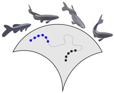
Our approach possesses the following contributions: (1) A unified Lie group-based paradigm is proposed to address the problems of pose estimation, tracking, and action recognition of articulated objects from depth images. As illustrated in Fig. 1, a 3D pose of an articulate object corresponds to a point in the underlying pose manifold, a long-time track of its 3D poses amounts to a long curve in the same manifold, whilst an action is represented as a certain curve segment. Therefore, given a depth image input, pose estimation corresponds to inferring the optimal point in the manifold; Action recognition amounts to classifying a curve segment in the same manifold as a particular action type; Meanwhile for the tracking problem, Brownian motion on Lie groups is employed as the generator to produce pose candidates as particles. This paradigm is applicable to a diverse range of articulated objects, and for this reason it is referred to as Lie-X. (2) Learning based techniques are incorporated instead of the traditional Jacobian matrices for solving the incurred inverse kinematics problem, namely, presented with visual discrepancies of current results, how to improve on skeletal estimation results. More specifically, an iterative sequential learning pipeline is proposed: multiple initial poses are engaged simultaneously to account for possible location, orientation, and size variations, with each producing its corresponding estimated pose. They then pass through a learned scoring metric to deliver the final estimated pose. Note the purpose of the learned metric in our approach is to mimic the behavior of the practical evaluation metric. (3) Empirically our approach has demonstrated competitive performance on fish, mouse, and human hand from different imaging modalities, where it is also specifically referred to as e.g. Lie-fish, Lie-mouse, Lie-hand, respectively. The runtime speed of our pose estimation system is more than realtime — it executes at around 83-267 FPS (frame per second) on a desktop computer without resorting to GPUs. Moreover, new sets of annotated depth images and videos of articulated objects are created. It is worth noting that the depth imaging devices considered in our empirical context are also diverse, including structured illumination and light field technologies, among others. These datasets and our code are to be made publicly available in support of the open-source research activities. 111Our datasets, code, and detailed information pertaining to the project can be found at a dedicated project webpage http://web.bii.a-star.edu.sg/~xuchi/Lie-X.html..
2 Related Work
The recent introduction of commodity depth cameras has led to significant progress in analyzing articulated objects, especially human full-body and hand. In terms of pose estimation, Microsoft Kinect is already widely used in practice at the scale of human full-body, while it is still a research topic at human hand scale [45, 30, 52, 31, 43, 42, 54], partly due to the dexterous nature of hand articulations. [45] is among the first to develop a dedicated convolutional neural net (CNN) method for hand pose estimation, which is followed by [30]. [31] also utilizes deep learning in a synthesizing-estimation feedback loop. [54] further considers to incorporate geometry information in hand modelling by embedding a non-linear generative process within a deep learning framework. [52] studies and evaluates a theoretically motivated random forest method for hand pose estimation. A hierarchical sampling optimization procedure is adopted by [43] to minimize the error-induced energy functions, where a similar energy function is optimized via efficient gradient-based techniques in [42] for personalizing hand shapes to individual users. [39] instead casts hand pose estimation as a matrix completion problem with deeply learned features. Meanwhile, various tracking methods have been developed for full-body [19] and hand [32, 4, 36]. A particle swarm optimization (PSO) scheme is utilized in [32] to recover temporal hand poses by stochastically seeking solution to the induced minimization problem. A hybrid method is adopted in [36] that combines PSO further with the widely-used iterated closest point technique. [4] considers learning salient points on fingers, for which an objective function is introduced to jointly take into account of edges, flow and collision cues. [19] describes a tracking-by-detection [3] type method based on 3D volumetric representation. 3D action recognition has also drawn great amount of attentions lately [29, 25, 48, 37]. For example, [25] tackles action recognition using variants of recurrent neural nets. [37] considers a mapping to a view-invariant high-level space by CNNs and Fourier temporal pyramid. Moreover, the work of [29] discusses a method to jointly train models for human full-body pose estimation and action recognition using spatial temporal and-or graphs. On the other hand, it is a much harder problem when a color camera is used instead of a depth camera, such as [1], where pose estimation is formulated as a regression problem that is subsequently addressed by relevance vector machine and support vector machine. Now, let us look at the other two articulated objects to be described in this paper, i.e. fish and mouse. They are relatively simple in nature but are less studied. Existing literature [7, 11, 12] are mostly 2D-based, and the focus is mainly on pose estimation. [49] is a very recent work in analyzing group-level behavior of lab mice that relies on a simplified straight-line representation of a mouse skeleton. We also would like to point out that there are research efforts across object categories: [12] estimates poses of zebrafish, lab mouse, and human face; Meanwhile there are also works that deal with more than one problem, such as [29]. They have achieved very promising results as discussed previously. Our work may be considered as a renewed attempt to address related problems and work with a broad range of articulated objects under one unified principle. For more detailed overview of related works, interested readers may consult to the recent surveys [34, 10, 33, 5].
Lie groups [35] have been previously used in [46] for detection and tracking of relatively rigid objects in 2D, however this requires the expensive image warping operations. [40] reviews in particular the recent development of applying shape manifold based approaches in tracking and action recognition. Its application in articulated objects is relatively sparse. Lie algebraic representation is considered in [27] for human full-body pose estimation based on multiple cameras or motion captured data. Rather than resorting to the traditional Jacobian matrices as in [27], learning based modules are employed in our approach to tackle the the incurred inverse kinematics problem. [47, 48] also extract Lie algebra based features for action recognition. Instead of focusing on specific problem and object, here we attempt to provide a unified approach.
Part-based models have long been considered in the vision community, such as the pictorial structures [13], the flexible mixtures-of-parts [53], the poslet model [6], the deep learning model [44], among others. The most related works are probably [12, 41], where the idea of group action has been utilized. Moreover, multiple types of objects are also evaluated in [12] that focuses on the 2D pose estimation problem, while [41] is dedicated to 3D hand pose estimation. On the other hand, our approach aims to address these three related problems altogether in 3D, and we explicitly advocate the usage of Lie group theory. Note that the concept of pose indexed feature has been coined and employed in [14, 2]. In addition, learning based optimization has been considered in e.g. [50], although in very different contexts. Finally, the idea of learning the internal evaluation metric is conceptually related to the recent learning to rank approaches [9] in the information retrieval community for constructing ranking models.
3 Notations and Mathematical Background
The skeletal representation is in essence based on the group of rigid transformations in 3D Euclidean , a Lie group that is usually referred to as the special Euclidean group SE. In what follows, we provide an account of the related mathematical concepts that will be utilized in our paper.
An articulated object, such as a human hand, a mouse or a fish, is characterized in our paper by a skeletal model in the form of a kinematic tree that contains one or multiple kinematic chains. As illustrated in Fig. 2, a fish or a mouse skeleton both possess one kinematic chain, while a human hand contains a kinematic tree structure of multiple chains. Note that only the main spine is considered herein for the mouse model. The skeletal model is represented in the form of joints interconnected by a set of bones or segments of fixed lengths. Empirical evidence has suggested that it is usually sufficient to use such fixed skeletal models with proper scaling, when working with pose estimation of articulated objects in depth images [41]. The pose of this object can thus be defined as a set of skeletal joint locations. Furthermore, we define the home position of an articulated object as a set of default joint locations. Taking a mouse model as depicted in the middle panel of Fig. 2 for example, its home position could be a top-view upward-facing mouse with the full body straight-up, and the bottom joint at the coordinate origin. Note this bottom joint contains 6 degrees of freedom (DoF) of the entire object, and is also referred to as the base joint. Then the pose could also be interchangeably referred to as the sequence of SE transformations or group actions applied to the home position, . The estimated pose is denoted as to better differentiate from the ground-truth pose. Here could be either or (to be discussed later) when without confusion in the context. To simplify the notation, we assume a kinematic chain contains joints. Clearly for fish and mouse models, while for human hand or human full-body, by focusing on one of the chains. A depth image is not only a 2D image but also a set of 3D points (i.e. a 3D point cloud) describing the surface profile of such object under a particular view. Ideally the estimated pose (the set of predicted joint locations) is expected to align nicely with the 3D point cloud of the object in the observed depth image.

Before proceeding further with the proposed approach, let us pause for a moment to have a concise review of the involved mathematical background. Motivated readers may refer to [28, 18, 23] for further details.
Lie Groups
A Lie group is a group as well as a smooth manifold such that the group operations of and are smooth for all . For example, the rotational group SO is identified as the set of 3 3 orthonormal matrices , with denoting the transpose, det being the determinant, and being a 3 3 identity matrix. Another example is SE, which is defined as the set of rotational and translational transformations of the form , with SO and . In other words, is the 4 4 matrix of the form
| (3) |
where . Note the identity element of is the 4 4 identity matrix . Both and will be simply denoted as if there is no confusion in the context. Now given a reference frame, a rigid-body transformation of two consecutive joints and in a kinematic chain can be represented as Moreover the product of multiple SE groups (i.e. a kinematic chain) is still a Lie group. In other words, as tree-structured skeletal models are considered in general for articulated objects, each of the induced kinematic chains forms a Lie group.
Lie Algebras and Exponential Map
The tangent plane of Lie group SO or SE at identity is known as its Lie algebra, or , respectively. An arbitrary element of so admits a skew-symmetric matrix representation parameterized by a three dimensional vector as
| (7) |
In other words, the DoF of a full SO is three. Note that a rotational matrix can alternatively be represented by the Euler angles decomposition [28]. A bijective mapping and its reverse mapping are defined as , and , respectively. Let , an element of se can then be identified as
| (10) |
With a slight abuse of notation, similarly there exist the bijective maps , and , with .
Now a tangent vector (or its matrix form ) is represented as ,
with indexing the -th component of .
Here , , , or in their respective matrix forms,
The exponential map in our context is simply the familiar matrix exponential for any . From the Rodrigues’s formula, it can be further simplified as
| (11) |
with
| (12) |
where is the vector norm.
It has been known in the screw theory of robotics [28] that every rigid motion is a screw motion that can be realized as the exponential of a twist (i.e. a infinitesimal generator) , with its components and corresponding to the angular velocity and translation velocity of the segment (i.e. bone) around its joint, respectively.
Product of Exponentials and Adjoint Representation
Consider a partial kinematic chain involving joints with , which becomes the full chain when . With a slight abuse of notation, let be the Lie group action on the partial kinematic chain, and or simply be the group action on the -th joint. Its forward kinematics can be naturally represented as the product of exponentials formula, . Therefore, for an end-effector from the home configuration (or home pose) , its new configuration is described by As discussed in [28], this formula can be regarded as a series of transformations from the body coordinate (for local joint) of each joint to the spatial coordinate (for global kinematic chain). Let us focus on a joint and denote and the twists of this joint in the body and spatial coordinates, respectively. Assume the transformation of this joint to the spatial coordinate is . The two twists can be related by the adjoint representation
which is obtained by
and repeatedly applying the identity for and .
Geodesics
Given two configurations and , the geodesic curve between them is with , , , and . Here the logarithm map or its simplified notion can be regarded as the inverse of the exponential map.
Brownian Motion on Manifolds
We refer interested readers to [18] for a more rigorous account of Brownian motion and stochastic differential geometry as they are quite involved. Here it is sufficient to know that Brownian motion can be regarded as a generalization of Gaussian random variables on manifolds, where the increments are independent and Gaussian distributed, and the generator of Brownian motion is the Laplace-Beltrami operator. In what follows we will focus more on the computational aspect [26]. Let denote a continuous variable, and be a small step size. Let denote a random vector sampled from normal distribution , for with being a covariance matrix. Then a left-invariant Brownian motion with starting point can be approximated by
| (13) |
In addition, these sampled points can be interpolated by geodesics to form a continuous sample path. In other words, for we have
| (14) |
4 Our Approach
In what follows we describe the proposed Lie-X approach for pose estimation, tracking, and action recognition of various articulated objects.
Preprocessing & Initial Poses
For simplicity we assume that there exists one and only one articulated object in an input depth image or patch. A simple preprocessing step is employed in our approach to extract individual foreground objects of interest. This corresponds to the point cloud of the object of interest extracted from the image. We then estimate the initial 3D location of base joint as follows: The 2D location of the base joint is set as the center of the point cloud, while its depth value is the average depth of the point cloud. Initial poses are obtained by first setting these poses as the home pose of the underlying articulate object, i.e. bones of the object are straight-up for the three empirical applications. For each of the initial poses, the initial orientation of the object is generated by perturbing the in-plane orientation of the above-mentioned base joint from a uniform distribution over . To account for the size variations, the bone lengths of each initial pose estimate are also scaled by a scalar that is uniformly distributed in the range of [0.9, 1.1].
Skeletal Models
After preprocessing, an initial estimated pose is provided for an input depth image. The objects of interest are represented here in terms of kinematic chains. Without loss of generality, in this paper we focus on fish and mouse that both have one chain, as well as human hand that possesses multiple chains, as depicted in the respective panels of Fig. 2. Our fish and mouse models contain 21 and 5 joints (including the end-effectors) along the main spine, respectively, while our hand model has 23 joints. Their corresponding DoFs are 25, 12, and 26, respectively. Overall our models are designed as proper approximations following the respective articulate objects’ anatomies. The base joint is fixed at coordinate origin which always has six DoFs describing 3D locations and orientations of the entire object; One DoF joints are applied to the rest fish joints characterizing the yaw of fish bones; Two DoFs are used for the rest mouse joints to account for both yaw and pitch; Similarly in our human hand model, two DoFs are used for each root joint of finger chain, while one DoFs are used for the rest joints. In all three models, zero DoFs are associated with the end-effectors, as each of them can entirely be determined by the preceding joints of the chain. Note that although simplified, the mouse model includes the most essential components (joints of the spine) at a reasonable resolution in our study. Our human hand model follows that of the existing literature (e.g. [31, 52]) that works with the widely-used NYU hand depth image benchmark [45].
4.1 Pose Estimation
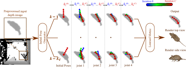
Fig. 3 provides a visual mouse example that illustrates the execution pipeline of our pose estimation procedure at test run. This is also presented more formally in Algorithm 1. Meanwhile the corresponding training process is explained in Algorithm 2. Note that inside both the training and testing processes, an internal evaluation metric or scoring function is used, which is also learned from data. In what follows we are to explain each of the components in detail.
Given a set of training images, define
| (15) |
the mean deviation over training images for the -th joint of the set of joints. The deviation characterizes the amount of changes between the estimated pose and the ground-truth pose, with its concrete form to be described later. A global error function can be defined over a set of examples that evaluates the sum of differences from the mean deviation, as for example the following form,
| (16) |
with being the standard vector norm in Euclidean space. Presented with the above visual discrepancies of current results, our aim here is to improve skeletal estimation results. Traditionally Jacobian matrices are employed for solving the incurred inverse kinematics problem. Here we instead advocate the usage of an iterative learning pipeline as displayed in Fig. 3 with a mouse example. At test run, it behaves as follows: Assume for each of the joints there are rounds or iterations. As presented in Algorithm 1, given a test image and an initial pose estimation, for each joint following the kinematic chain of length from the base joint, at current round , the current pose of the joint will be corrected by the Lie group action , with the twist being the output of a local regressor, . In other words, denote the short-hand notations , , and , The -th joint spatial coordinate can be updated by the following left group action
| (17) |
with being the latest group element used to further correct the spatial location of -th joint at round . It is worth emphasizing that this process requires learning the set of local regressors , where the output of each regressor, , is dedicated to a particular round and joint . Each of these local models is learned based on local features, i.e. the pose-indexed depth features to be described later. In a sense, it endows our system with the ability to memorize local gradient updating rules from similar training patterns. This essentially forms the key ingredient that allows for removal of the commonly used Jacobian matrices for error-prorogation in our approach. Moreover, at test run, multiple initial poses are generated for each input image. They will then pass through our learned inverse kinematic regressors and produce corresponding candidate poses. These output poses will nevertheless be screened by our learned metric to be discussed later, where the optimal one is to be picked as the final estimated pose.
At training stage, a set of initial poses of the input image is obtained in the same manner as those of the testing stage. The aforementioned local regressors are then learned as follows. Each example of the training dataset consists of an instance: a pair of poses including the estimated pose and the ground-truth pose, , as well as its label: the deviation of estimation from ground-truth , as
| (18) |
For the first joint (the base joint in the kinematic chain) and at the first round , the label of an example will be the amount of changes from the first joint of the initial pose to that of the ground-truth. Then at any round , its corresponding initial pose is obtained by executing the current partial kinematic model until the immediate previous round . Similarly for the second joint and at round , the initial pose in each of the training examples is attained by executing the current partial model from base joint up to round of the current joint, and its label is then the amount of changes from the current joint of the aforementioned initial pose to the second joint of the ground-truth. In this way, the training examples are prepared separately over joints and then across rounds until the very last joint round . Algorithm 2 presents the procedure of learning the set of regressors , with each regressor of round and joint being learned from its local context to make its prediction, . Without loss of generality the random forest method [8] is engaged here as the learning engine.
Note that our hand skeletal model contains five kinematic chains, all of which share the hand base joint as root of the tree. For each chain, the sub-chain resulting from the exclusion of the base joint is independent of the other sub-chains given that the root is set. This motivates us to consider the following procedure: At test run, the base joint is first worked out, following the process described above. After this is done, Algorithm 1 is executed for each of the five sub-chains separately.
Learning the Internal Evaluation Metric
Since multiple pose hypotheses are presented in our approach, it remains to decide on which one from the candidate pool we should choose as the final pose estimate. Traditionally this can be dealt with by either mode seeking or taking their empirical average as in e.g. Hough voting methods [17, 24, 15] or random forests [8], respectively; It could also be carried out by simply matching with a small set of carefully crafted templates such as distance transform or DOT [16]. Instead we propose to learn a surrogate scoring function that is to be consistent with the real evaluation metric employed during practical quantitative analysis. This learned scoring function then becomes a built-in module in our approach to select the pose hypothesis with the least error.
More concretely, the widely used criteria of average joint error [51] is adopted as the evaluation metric for our scoring function to mimic. During training stage, a set of training examples are generated, where a training example consists of an instance and a label: A training instance contains an input depth image, its ground-truth pose (i.e. skeletal joint locations) and an estimated pose as a set of corresponding joint locations after random perturbations from the ground-truth. Its label is the average joint error between the estimated and the ground-truth poses. Therefore a second type of regressor, , is utilized here to learn to predict the error at test run. Namely, given an unseen depth image and an estimated pose, our regressor would produce a real-valued score mimicking the average joint error as where the ground-truth is known.
4.2 Tracking
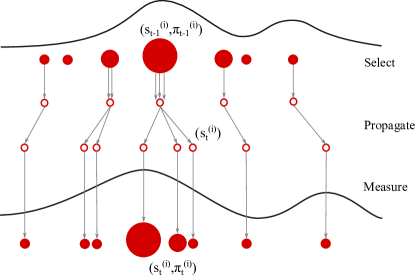
Particle filters such as [20] have long been regarded as a powerful mean for tracking, and is also considered in our context to address the tracking problem. To facilitate a favorable balance between efficiency and effectiveness, we consider a probabilistic particle filter based approach only for the base joint, where particles are formed by Brownian motion based sampling in the pose manifold; Meanwhile the parameters of the remaining joints are obtained by invoking the same inference machinery as in our deterministic pose estimation algorithm. This design is also motivated from our empirical observation that often the object poses are also well-estimated when the prediction of the base joint is in close vicinity of the true values. That is, according to our observation the first joint is crucial in pose estimation: If is wrongly predicted, estimation results of the remaining joints could be seriously damaged; When our prediction of is accurate, the follow-up joints estimates would also be accurate. Algorithm 3 further presents the main procedure for our tracking task, which is also visually illustrated in Fig. 4, with a detailed description in the following paragraphs.
Following the particle filter paradigm [20] we consider a discretized time step , and use to denote a latent random variable as well as for its observation. Here the state of a tracked object (i.e. the estimated pose at time ) is denoted as and its history is . Similarly, current observation is denoted as , and its history as . The underlying first-order temporal Markov chain induces conditional independence property, which by definition gives . Following the typical factorization of this state-space dynamic model, we have
with . We also need the posterior probability for filtering purpose, which in our context is defined as , with . In other words, it is evaluated by considering the posterior from the previous time step in a recursively manner.
The realization of the particle filter paradigm in our context involves the three-step probabilistic inference process of selection-prorogation-measurement, which serves as the one time-step update rule in particle filter, and is also described in Algorithm 3. Specifically, the process at current time-step corresponds to an execution of the selection-prorogation-measurement triplet steps: The output of previous time-step contains a set of weighted particles
Here each particle , , corresponds to a particular realization of the set of tangent vector parameters that uniquely determines a pose, where each of the vectors is attached to a joint following the underlying kinematic chain. The particle is also associated with its weight . Collectively this set of weighted particles is thus regarded as an approximation to the posterior distribution . The selection step operates by uniform sampling from the cumulative distribution function (CDF) of to produce a new set of particles with equal weights. It is followed by the propagation step where the manifold-based Brownian motion sampling of Eq.(14) is employed to realize , i.e. to obtain the new state based on discretized Brownian motion deviation from the previous time-step. Note that this Brownian motion sampling is carried out only on the base joint, while the remaining joints are obtained by directly executing the same inference machinery of Eq.(17) as in our pose estimation algorithm. Now, the sample set constitutes an approximation to the predictive distribution function of . The measurement step finally provides an updated weight for each particle as follows: Let be the predicted error value of the -th particle , obtained by applying our learned metric. The weight is thus evaluated as
| (19) |
After obtaining all the weights, each of the weights, , is further normalized as
| (20) |
The updated sample set now collectively approximates the corresponding posterior distribution at time .
The set of weighted particles allows us to represent the entire distribution instead of a point estimate as what we have done during the pose estimation task. The final pose estimate, (i.e. at time ), is produced by weighted averaging over this set of particles,
| (21) |
4.3 Action Recognition
Our approach can be further employed to work with the problem of action recognition. The key insight is that an action instance (i.e. a pose sequence) corresponds to a curve segment in the manifold, whereas the set of all instances of a particular action type corresponds to a group of curves. Therefore, the task of action recognition can be cast as separating different groups of action curves. It motivates us to consider a third type of learned predictor, . Here dedicated features are extracted as to be described next, and the output concerns that of predicting its action categories.
Action Recognition Features
As the length of action sequences may vary, they are firstly normalized to the same length (in practice 32 frames) using linear interpolation. Local features from each frame of a sequence can be obtained based on the tangent vectors (Lie algebras) of the estimated joints in the manifold. Each temporal sequence is further split into 4 equal-length segments, where the frames in a segment collectively contain the set of tangent vectors as local features. Moreover, a temporal pyramid structural representation is utilized in a sense similar to that of the spatial pyramid matching [22], where features are extracted using hierarchical scales of {4,2,1}, where corresponds to the 4 segments introduced previously, and the rest correspond to those coarser scales built over it layer by layer. In total it leads to 7 temporal segments (or sets of variable sizes) over these 3 scale spaces. For each such segment, the mean and standard deviation of its underlying pose representation (in terms of Lie algebras to be described below) are then used as features. Now let us investigate the details of these pose representations defined on single frames, which can be decomposed into joints following the aforementioned kinematic chain structure. For the base joint, we use the Lie algebras of the transformation from the current frame to the next frame. For the rest of the joints, we use the Lie algebras of the transformation from previous joint to the current joint and that of the transformation from current frame to the next frame. Besides, we also use the 3D location and orientation of the first joint (i.e. base joint) as features. In particular for fish-related actions, rather than using the Lie algebras of all 20 joints, we emphasize on robust estimation by considering a compact feature representation: The first component or sub-vector of the feature vector corresponds to the Lie algebra of the base joint; The second and the third components are the sub-vectors of the same length obtained by averaging over the set of Lie algebras from second to tenth joints, and from eleventh to the last joint, respectively. Overall a 252-dim feature vector is thus constructed to fully characterize an action sequence.
4.4 Random Forests, Pose-indexed Depth features, and Binary Tests
There are three types of learned predictors (namely the set of local regressors , the learned internal metric , and the action recognition predictor ) considered in our approach. In general any reasonable learning method can be used to realize these three types of predictors. In practice the random forest method [8, 15] is engaged for these learning tasks, so it is worthwhile to describe its details here.
For action recognition, a unique set of action features are used as stated previously. In what follows, we thus focus on the description of our pose-indexed depth features, which are used in the first two types of regressors, , and . Our feature representation can be regarded as an extension of the popular depth features as discussed in [38, 51] by incorporating the idea of pose-indexed features [14, 2] to model 3D objects. We start by focusing on a joint with its current 3D location , where a 3D offset can be obtained by random sampling from the home pose. Let denote the Lie group left action of current object pose applied onto . Now the 3D location of the offset is naturally , and its projection onto 2D image plane under current camera view is denoted as . Similarly we can obtain another random offset . For a 2D pixel location of an image patch containing the object of interest, its depth value can be denoted as . Now we are ready to construct a feature or its short-hand notation , by considering two 2D offsets positions from :
| (22) |
Due to the visibility constraint, we are only able to obtain the depth values of the projected 2D locations and from the object surface. Thus is a surjective map. Nevertheless, this serves our intention of sampling random features well. Following [8], a binary test is defined as a pair of elements, , with being the feature function, and being a real-valued threshold. When an instance with pixel location passes through a split node of our binary trees, it will be sent to the left branch if , and to the right side otherwise.
Our random forest predictors are constructed based on these features and binary tests for split nodes. Similar to existing regression forests in literature including e.g. [38], at a split node, we randomly select a relatively small set of distinct features as candidate features. For every candidate feature, a set of candidate thresholds is uniformly selected over the range defined by the empirical set of training examples in the node. The best test is chosen from these features and accompanying thresholds by maximizing the following gain function. This procedure is then repeated until there are levels in the tree or once the node contains fewer than training examples. More specifically, the above-mentioned split test is obtained by
where the gain is defined as:
| (23) |
Here denotes the cardinality of the set, denotes the set of training examples arriving at current node, which is further split into two subsets and according to the test . Define the mean deviation of the set to -th joint, and accordingly for and . The function is defined over a set of examples that evaluates the sum of differences from the mean deviation:
| (24) |
In the final decision stage, for the first two regression modules, the mean-shift mode searching in Hough voting space is used as e.g. in [15], while for the third module (action recognition) the classical random forest strategy [8] is used to pick the category with largest counts from the averaged histogram.
5 Empirical Evaluations
Empirically our Lie-X approach is examined on three different articulated objects: fish, mouse, and human hand.
Performance Evaluation Metric
Our performance evaluation metric is based on the commonly-used average joint error, computed as the averaged Euclidean distance in 3D space over all the joints. Formally, let and be the ground-truth and estimated joint locations, respectively. The joint error of the pose estimate is defined as , where is the Euclidean norm in 3D space. When dealing with test images, let index over the test images, and their corresponding joint errors denoted as . The average joint error is then defined as .
Internal Parameters
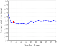
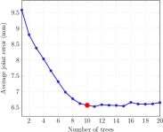
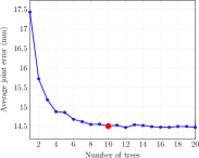
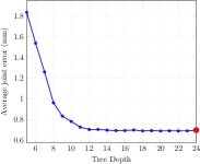
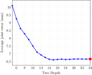
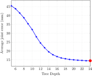
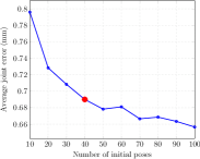
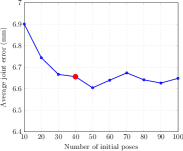
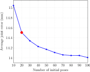
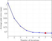
Throughout experiments, a fixed set of values is always used for the internal parameters of our approach, unless otherwise stated, as follows. For the the first type of regressors (namely the set of local regressors ), the number of trees is fixed to (3, 10, 10), while the tree depth is (24, 24, 24) for the triplet of articulated objects (fish, mouse, hand), respectively. For the second type (the learned internal metric ), the number of trees is (20, 20, 20), while the tree depth is (15, 15, 20) for the triplet of articulated objects (fish, mouse, hand), respectively. For the third type (the action recognition predictor) , the number of trees in the forest is 50, and tree depth is 20. The number of features is =8,000, and the maximum number of examples in the leaf node is =5. The number of rounds at each joint is set to =7, 3, and 3, for fish, mouse, and hand, respectively. The local image patch sizes considered in our approach for fish, mouse, and hand are normalized to , , mm2, respectively. These patches are used as input to the local random forest regressors in our approach to estimate the spatial coordinate of next joint based on current joint following the kinematic chain. One important parameter is , the number of initial poses in pose estimation. In practice, after factoring-in the efficiency consideration, is set to 40, 40, 20 for pose estimation of fish, mouse, and hand, respectively, throughout experiments. Similarly, the number of initial poses for tracking is set to =200. For learning the internal evaluation metric, the number of candidates is set to 8. Namely, given a training dataset of size , the number of training examples for pose estimation becomes , while the number of training examples for learning the internal metric is .
| Fish | Mouse | Hand | |
| Number of trees | |||
| Tree depth | |||
| Number of initial poses | |||
| Number of iterations | |||
| Number of trees for learning internal metric |
5.1 Datasets
To examine the applicability of our approach on diverse articulated objects, we demonstrate in this paper its empirical implementation for fish, mouse, and human hand, respectively, where three distinct real-life datasets are employed. In particular, here we introduce our home-grown 3D image datasets of zebrafish and lab mouse that are dedicated to the related problems of pose estimation, tracking, and action recognition. The images have been captured and annotated by experts to provide the articulated skeleton information describing the pose of the subject. The popular NYU hand depth image dataset [45] is also considered here. More details of the datasets are discussed next. It is worth noting that different imaging modalities are utilized across the three datasets: light-field depth images are used for fish, while structured illumination depth cameras are employed for mouse and human hand objects. Regardlessly our approach is demonstrated to work well across these diverse image modalities.
Our Fish Dataset
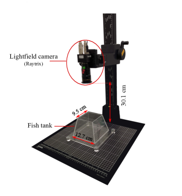
Depth images are acquired with a top-mount Raytrix R5 light-field camera at a frame rate of 50 FPS and a resolution of , as displayed in Fig. 5(a). The depth images are obtained from the raw plenoptic images by utilizing Raytrix on-board SDK. In total 7 different adult zebrafish of different genders and sizes are engaged in our study. From the captured images, 2,972 images containing distinct poses are annotated. The training dataset of 95,104 images is thus formed by augmenting each fish object of these images with 31 additional transformations, where each transformation comes with a random scaling within [0.9, 1.1] and with a random in-plane rotation within (-, ). The test dataset of pose estimation problem contains 1,820 distinct fish images.
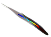
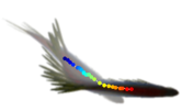
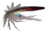
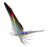
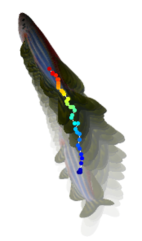
In addition to single-frame based pose annotations, we also record, annotate, and make available a fish action dataset. [21] provides a comprehensive catalogue of zebrafish actions, from which a subset of 9 action classes are considered in this paper, which is listed below as well as illustrated in Fig.19:
- Scoot:
-
Moves along a straight line.
- J-turn:
-
Fine reorientation during which the body slightly curves , with a characteristic bend at the tail.
- C-turn:
-
Fish body curves to form a C-shape en route to a near turn.
- R-turn:
-
Involves routine angular turn of greater than .
- Surface:
-
Moves up towards the water surface.
- Dive:
-
Moves towards the tank bottom.
- Zigzag:
-
Contains erratic movements with multiple darts in various directions.
- Thrash:
-
Consists of forceful swimming against the side or bottom walls of the tank.
- Freeze:
-
Refers to complete cessation of movement.
Our fish action dataset contains 426 training sequences and 173 testing sequences, respectively, from 7 different fish over the aforementioned 9 categories. The length of each fish action sequence varies from 7 frames to 135 frames.
Our Mouse Dataset
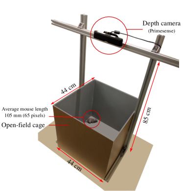
Mouse depth images are collected using a top-mount Primesense Carmine depth camera at a frame rate of 30 FPS and with a resolution . Fig. 5(b) presents our dedicated imaging set-up. Two different lab mouse are engaged in our study. We select 3,253 images containing distinct poses and depth noise patterns, and augment them with additional transformations following the same protocol as above, which gives rise to the training dataset here containing 104,096 images. The testing dataset of pose estimation problem contains 4,125 distinct depth images. For tracking problem, the test set consists of two sequences of length 511 and 300 frames, respectively.
The NYU Hand Dataset
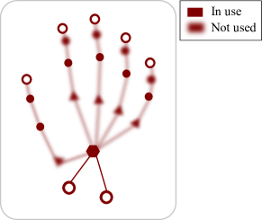
We also evaluate our approach on the benchark NYU hand depth image dataset[45] 222The NYU dataset is publicly available at http://cims.nyu.edu/~tompson/NYU_Hand_Pose_Dataset.htm.. It contains 72,757 depth images for training and =8,252 frames for testing. All images are depth images captured by Microsoft Kinect using the structured illumination technique, which is the same as the Primesense camera used in our mouse dataset. Depth images in the training set are from a single user, while images in the test set are from two users. While a ground-truth hand label contains 36 annotated joints, only 14 of these joints are considered in many existing efforts using this dataset, such as [45, 30, 31, 54], which is followed during our experiments. This is also presented in Fig. 6: Important hand joints are included in this subset of 14 joints, such as all the finger tips and the hand base.
| Comparison methods on articulated objects | fish | mouse |
|---|---|---|
| RF | 1.28 | 12.24 |
| CNN | 0.79 | 9.17 |
| Lie-X (w/o multiple initial poses) | 3.28 | 13.27 |
| Lie-X (w/o learned metric) | 1.71 | 9.82 |
| Lie-X | 0.68 | 6.64 |
| Comparison methods on hand pose estimation | average joint error (mm) |
|---|---|
| RF | 24.81 |
| CNN | 18.82 |
| Tompson et. al. [45] | 21.00 |
| Oberweger et. al. [30] | 20.00 |
| Oberweger et. al. [31] | 16.50 |
| Zhou et. al. [54] | 16.90 |
| Lie-X (w/o multiple initial poses) | 20.50 |
| Lie-X (w/o learned metric) | 16.72 |
| Lie-X | 14.51 |
5.2 Pose Estimation of Fish, Mouse, and Human Hand
In this subsection, we focus on the problem of pose estimation for articulated objects such as fish, mouse, and hand. To make a fair comparison with existing methods, we specifically implement two non-trivial baseline methods, namely regression forest (RF), and convolutional neural network (CNN). The RF method is a re-implementation of the classical regression method used by Microsoft Kinect [38], with the only difference being that our RF implementation explicitly utilizes a skeletal model, instead of estimating joint locations without skeletal constraints as in [38]. Two separate regression forests, and , are trained for this purpose. Here is used to estimate the 3D location and in-plane orientation of the subject, followed by which produces a set of 3D pose candidates. The number of trees trained are set to 7 and 12 for and , respectively. In both cases, the maximum tree depth is fixed to =20. The standard depth invariant two-point offset features of [38] are also used. The CNN method is obtained as follows: The pre-trained AlexNet CNN model from ImageNet is engaged as the initial model. To tailor the training data for our CNN, objects of interest from the training depth images are cropped according to their bounding boxes. The depth values in each patch are rescaled to be in the range of 0 to 255. Each object patch is replicated three times to form into a RGB image, which is then resized as an input instance of size 224 224. This together with its corresponding annotation prepares a training example. Then our CNN model is finally obtained by executing the MatConvNet package to train on these training examples for 50 epochs.
Sensitivity Analysis of the Internal Parameters
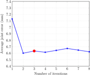
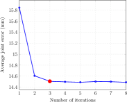
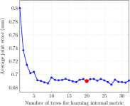
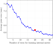
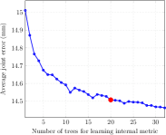
As our approach contains a number of internal parameters, it is of interest to systematically investigate the influence of these parameters w.r.t. the final performance of our system. Here we consider five influential parameters, which are the number of initial poses , the number of rounds , the number and depth of trees in our first type of regressors (i.e. the local regressors ), as well as the number of trees used in our learned metric component . Fig. 7 displays the performance of Lie-X with respect to each of these five parameters row-by-row. Meanwhile each of the three columns presents the respective results for fish, mouse, and hand. Each of the fifteen panels in this five by three matrix is obtained by varying one parameter of interest while keeping the other parameters fixed to default values. In general, our system behaves in a rather stable manner w.r.t. the change of internal parameters over a wide range of values. Moreover, in each of the panels, a red colored dot is placed to indicate the specific parameter value empirically employed by our approach in this paper. It is worth noting that the choice of these internal parameter values represents a compromise between performance and efficiency.
| Comparison methods | uses GPU | frames per second (FPS) |
|---|---|---|
| Tompson et. al. [45] | ✓ | 30 |
| Oberweger et. al. [30] | ✓ | 5,000 |
| Oberweger et. al. [31] | ✓ | 400 |
| Zhou et. al. [54] | ✓ | 125 |
| Lie-X | 123 |
| (a) Fish | (b) Mouse | (c) Hand | ||||||

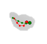
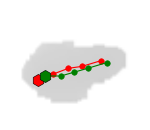
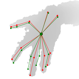
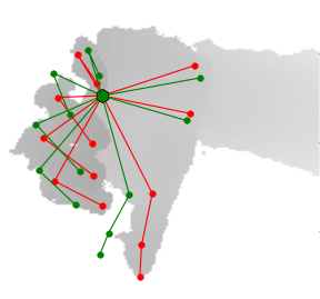
Comparison with Baselines and the State-of-the-art Methods
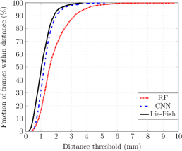
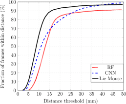
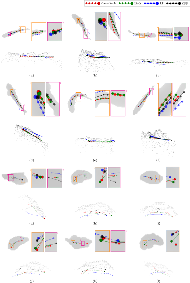
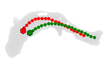
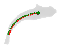
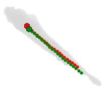
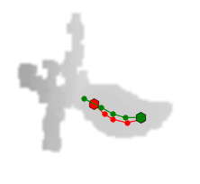
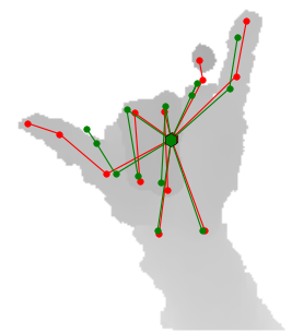
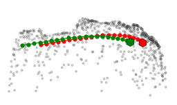
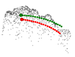
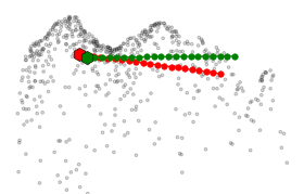
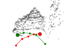
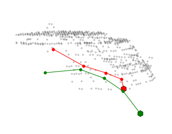
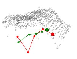
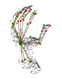
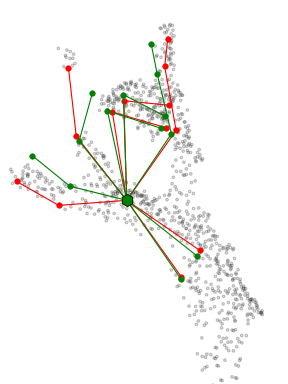
To evaluate the performance of the proposed approach, a series of experiments are conducted on the aforementioned datasets for fish, mouse, and hand pose estimation tasks. Table 1 presents a comparison of Lie-X w.r.t. the two non-trivial baseline methods (i.e. RF and CNN) on fish and mouse pose estimation tasks. Overall, our approach clearly outperforms the others by a significant margin, while CNN achieves better results over RF. Moreover, the error distributions of these comparison methods are also presented in Fig. 8(a-b), where our approach clearly outperforms the baselines most of the time. The superior performance of our Lie-X approach is also demonstrated in Fig. 9, which provides visual comparisons of pose estimation results for six fish and six mouse examples, respectively, over the three competing methods. From these visual examples, it is observed that the estimated poses from our Lie-X approach tend to be more faithfully aligned with the ground-truth when compared against the two baseline methods.
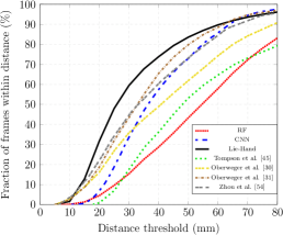
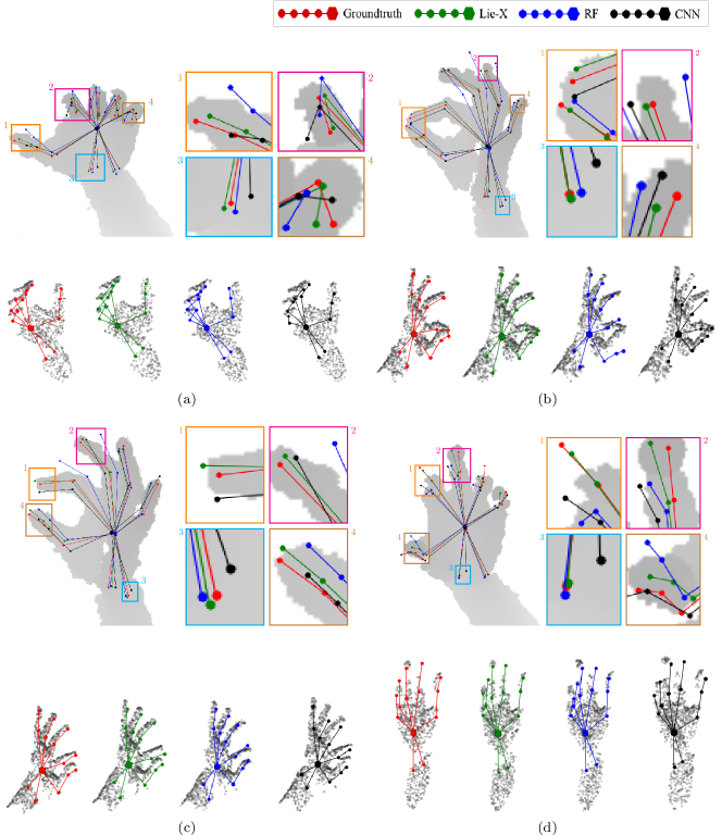
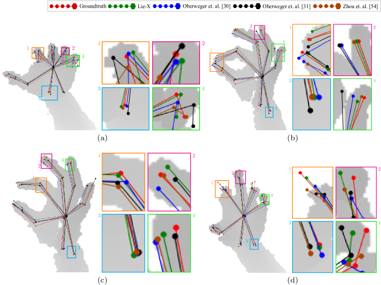
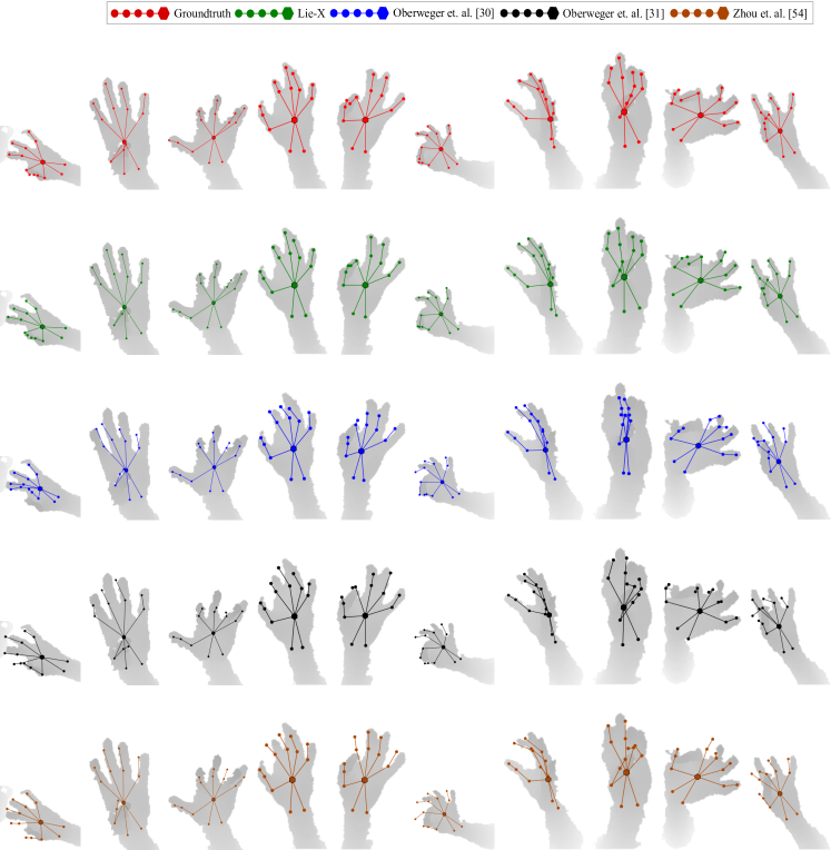
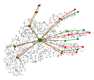
Our approach is also validated on the NYU hand depth benchmark, as is displayed in Table 2. Overall, our CNN baseline result is on par with the standard deep learning results of e.g. [30] that also utilizes a AlexNet-like CNN. This helps to establish that our baselines are consistent in terms of performance with what has been reported in the literature, which are also used as pose estimation baselines on fish and mouse objects. Moreover, the results of the state-of-the-art methods are also directly compared here, including Tompson et. al. [45], Oberweger et. al. [31], and Zhou et. al. [54]. It is worth pointing out that the test error rate of our approach is 14.51 mm in terms of average joint error. This is by far the best result on hand pose estimation task to our knowledge, which improves over the best state-of-the-art result of 16.50 mm of [31] by almost 2 mm. More detailed quantitative information is revealed through the error distributions of comparison methods in Fig. 8(c), where our approach clearly outperforms the baselines and the state-of-the-art methods. Similarly, visual comparison results are provided in Fig. 10, Fig. 11, and Fig. 10, where our approach is again shown to clearly outperform other methods. More specifically, Fig. 10 and Fig. 11 present the visual results of all competing methods on the same four exemplar hand images. Due to the access limit, we are only able to present the side-view results on our approach and the baseline methods of RF and CNN. Fig. 10 provides additional visual results comparing our approach to state-of-the-arts on ten more hand images.
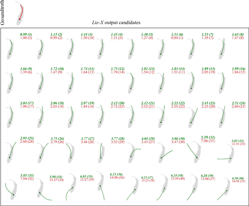
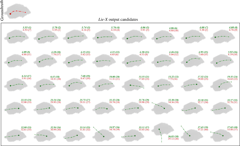
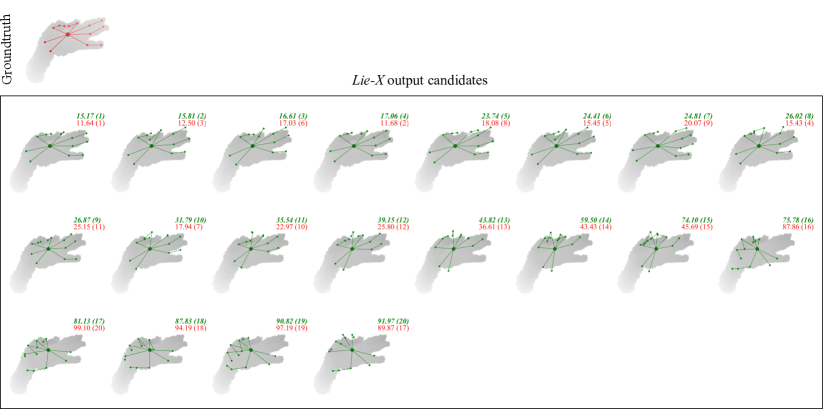
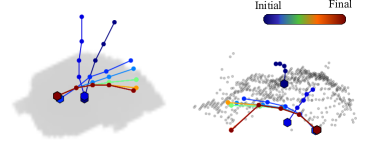
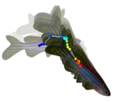
To reveal the inner working of our approach, in Fig. 13, Fig. 14, and Fig. 15, a visual example is respectively provided for pose estimation of fish, mouse, and hand. It is evident that a diverse set of pose candidates are obtained that covers distinct pose location, orientation, and sizes. This is made possible due to the adoption of multiple initial poses. Moreover, prediction scores and associated orders from our learned metric module in general closely resembles that of the empirical evaluation metric. In addition, Fig. 16 presents several intermediate pose estimation results from different joints and rounds on an exemplar mouse image, when executing the pose estimation pipeline as illustrated in Fig. 3. It is observed that each step of the iterative process usually helps in converging toward the final pose estimation.
| (a) Scoot | (b) J-turn | (c) C-turn | |
| (d) R-turn | (e) Surface | (f) Dive | |
| (g) Zigzag | (h) Thrash | (i) Freeze |



With vs. Without Multiple Initial Poses
As presented in Table 1 for fish and mouse objects and Table 2 for hand objects, empirically we observe that the presence of multiple initial poses always improves the pose estimation performance. As presented in Figs. 13, 14, and 15, execution of our pose estimation process, starting from multiple distinct initial poses, results in unique pose estimates, each of which can be regarded as a locally optimal result. This is due to the highly non-convex nature of our problem, a well-known fact for systems of rigid-bodies in general. These visual examples also demonstrate the importance of having multiple initial poses to avoid getting trapped into local optimal points that are far from the ground-truth point.
With vs. Without the Learned Metric
To examine the usefulness of our learned internal metric, a special variant of our approach without this component is engaged here, which is also referred to as Lie-X w/o learned metric. Provided with multiple output pose candidates, this variant differs from our full-fledged approach by averaging over them for each of the joints in the 3D Euclidean space, instead of scoring them with the learned metric to pick up the best estimate. Empirical experiments such as those presented in Table 1 for fish and mouse objects and Table 2 for hand objects suggest a noticeable performance degradation when without the learned metric. Clearly the learned internal metric does facilitate in selecting from a global viewpoint the final estimate, which is obtained from the pool of locally optimal candidates using multiple initial poses. It has also been demonstrates in Figs. 13, 14, and 15 that in our context a max operation (i.e. with the learned metric) may well outperform an average operation (i.e. w/o learned metric). In particular, visually our learned internal metric is capable of producing predicted error scores that are nicely aligned with the true average joint error when we have access to the ground-truth.
Computational Efficiency
All experiments discussed in this paper are performed on a desktop PC with an Intel i7-960 CPU and with 24Gb memory. At this moment, our CPU implementation achieves an average run-time speed of 83 FPS, 267 FPS, and 123 FPS for fish, mouse, and hand tasks, respectively. Table 3 summarizes the run-time speed comparisons with state-of-the-art hand pose estimators on the NYU hand dataset [45]. Our result of 123 FPS is obtained with only CPU access, nevertheless it is still comparable with most of these recent methods which are based on GPUs. Note the empirical runtime speed of our approach could be further improved by exploiting the computing power of modern GPUs. Meanwhile, an exceptionally high speed method is developed in Oberweger et. al. [30], which is made possible by the usage of very shallow neural nets. This however comes with degraded performance as shown in Table 2, with a significant average joint error increase of 5.41 mm when compared to our approach.
Common Pose Estimation Errors of Our Approach
Although our Lie-X approach performs relatively well in practical pose estimation settings, inevitably it does make mistakes in practical situations. These common errors include the following ones: orientation flips, displacement along the z-direction and sub-optimal shape fitting. A visual illustration of these common errors made by our approach is provided in Fig. 17. As can be observed, usually our Lie-Fish results are best aligned with the ground-truths. The mistakes of Lie-Mouse are more noticeable. Meanwhile the visual displacements of our Lie-Hand results from the ground-truths are most significant. This is to be expected, as the corresponding complexity levels of the three tasks varies from being relatively simple (i.e. kinematic chains) to complex (i.e. kinematic trees).
5.3 Tracking of Mouse
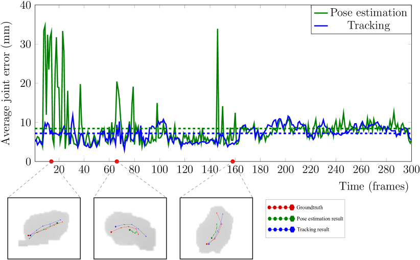
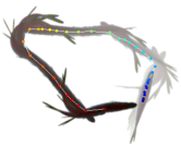
Our Lie-X approach is also examined on the tracking task using the mouse tracking dataset described beforehand. Compared with our single frame based pose estimation of Alg. 1, it is of interest to examine on how much we can gain from our tracking algorithm of Alg. 3, when temporal information is available. Empirically our mouse tracker is shown to produce an improved performance of 7.19 mm from the 8.42 mm results from our pose estimator on single frames. This can also be observed from the bottom row of Fig. 18 where visual comparisons are provides at several time frames. By exploiting temporal information, the results of our tracker are shown to produce less dramatic mistakes comparing to that of pose estimation. It is again evidenced quantitatively in Fig. 18, which presents a frame-by-frame average joint error comparison of tracking vs. pose estimation on a test sequence. Clearly there exists a number of very noisy predictions of pose estimation. In comparison our tracking results are in general much less noisy. Overall, the tracking results outperforms post estimation with a noticeable gap of at least 1 mm. Note the tracking results in some frames are slightly inferior to that of the pose estimation counterpart, which we attribute to the utilization of the averaging operations in our tracker.
5.4 Action Recognition of fish
To demonstrate the application of our approach on action recognition tasks, in what follows we conduct experiments on the aforementioned fish action dataset. In addition to the proposed tangent vector (i.e. Lie algebras) based feature representation, as comparison we also consider a joint based feature representation. Here the main body of the feature representation follows exactly as in the tangent vector representation, including e.g. the adoption of a temporal pyramid of , with the only change as follows: Instead of tangent vectors, the corresponding the 3D joint positions are employed. This finally leads to an 888-dim feature vector representation.
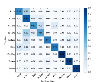
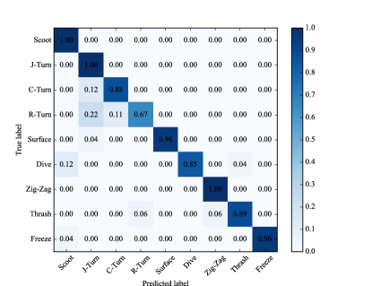
Fig. 19 displays our fish dataset that contains nine unique action categories. The standard evaluation metric of average classification accuracy are considered in this context. Empirically the comparison method that utilizing joint position features achieves a performance of 79.19%, which is significantly outperformed by our approach based on tangent vector features with the average accuracy of 91.33%. Fig. 20 provides further information of category-wise errors in the form of the confusion matrices. It is observed that the joint based method tends to confuse among the subset of actions of scoot, J-turn, c-turn, and r-turn, which are indeed more challenging to be separated due to their inherent similarities. Nonetheless, the performance on this subset is dramatically improved in our approach with tangent vector based features. We hypothesize that by following the natural tangent vector representation, our approach gains the discriminative power to separate these otherwise troublesome action categories.
6 Conclusion and Future Work
A unified Lie group approach is proposed for the related key problems of pose estimation, tracking, and action recognition of diverse articulated objects from depth images. Empirically our approach is evaluated on human hand, fish and mouse datasets with very competitive performance. For future work, we plan to work with more diverse articulated objects such as human full body and wild animals, as well as their interactions with other articulated objects and background objects.
Acknowledgment
The project is partially supported by A*STAR JCO grants 1431AFG120 and 15302FG149. Mouse and fish images are acquired with the help of Zoe Bichler, James Stewart, Suresh Jesuthasan, and Adam Claridge-Chang. Zilong Wang helps with the annotation of mouse data, while Wei Gao and Ashwin Nanjappa help with implementing the mouse baseline method.
References
- [1] Agarwal, A., Triggs, B.: Recovering 3D human pose from monocular images. IEEE Trans. PAMI 28(1) (2006)
- [2] Ali, K., Fleuret, F., Hasler, D., Fua, P.: Joint pose estimator and feature learning for object detection. In: ICCV (2009)
- [3] Andriluka, M., Roth, S., Schiele, B.: People-tracking-by-detection and people-detection-by-tracking. In: CVPR (2008)
- [4] Ballan, L., Taneja, A., Gall, J., Gool, L.V., Pollefeys, M.: Motion capture of hands in action using discriminative salient points. In: ECCV (2012)
- [5] Barsoum, E.: Articulated hand pose estimation review. Arxiv pp. 1–50 (2016)
- [6] Bourdev, L., Malik, J.: Poselets: Body part detectors trained using 3D human pose annotations. In: ICCV (2009)
- [7] Branson, K., Belongie, S.: Tracking multiple mouse contours (without too many samples). In: CVPR (2005)
- [8] Breiman, L.: Random forests. Machine Learning 45(1), 5–32 (2001)
- [9] Burges, C., Shaked, T., Renshaw, E., Lazier, A., Deeds, M., Hamilton, N., Hullender, G.: Learning to rank using gradient descent. In: ICML (2005)
- [10] Chen, L., Wei, H., Ferryman, J.: A survey on model based approaches for 2D and 3D visual human pose recovery. PRL 34(15), 1995–2006 (2013)
- [11] Dollar, P., Rabaud, V., Cottrell, G., Belongie, S.: Behavior recognition via sparse spatio-temporal features. In: IEEE Workshop on PETS (2005)
- [12] Dollar, P., Welinder, P., Perona, P.: Cascaded pose regression. In: CVPR (2010)
- [13] Felzenszwalb, P., Huttenlocher, D.: Pictorial structures for object recognition. International Journal of Computer Vision 61(1), 55–79 (2005)
- [14] Fleuret, F., Geman, D.: Stationary features and cat detection. JMLR 9, 2549–2578 (2008)
- [15] Gall, J., Yao, A., Razavi, N., van Gool, L., Lempitsky, V.: Hough forests for object detection, tracking, and action recognition. IEEE Trans. PAMI 33(11), 2188–2202 (2011)
- [16] Hinterstoisser, S., Lepetit, V., Ilic, S., Fua, P., Navab, N.: Dominant orientation templates for real-time detection of textureless objects. In: CVPR (2010)
- [17] Hough, P.: Machine analysis of bubble chamber pictures. In: Proc. Int. Conf. High Energy Accelerators and Instrumentation (1959)
- [18] Hsu, E.P.: Stochastic Analysis on Manifolds. AMS Press (2002)
- [19] Huang, C., Allain, B., Franco, J., Navab, N., Boyer, E.: Volumetric 3D tracking by detection. In: CVPR (2016)
- [20] Isard, M., Blake, A.: Condensation -— conditional density propagation for visual tracking. International journal of computer vision 29(1), 5–28 (1998)
- [21] Kalueff, A., Gebhardt, M., Stewart, A., Cachat, J., Brimmer, M., Chawla, J., Craddock, C., Kyzar, E., Roth, A., Landsman, S., Gaikwad, S., Robinson, K., Baatrup, E., Tierney, K., Shamchuk, A., Norton, W., Miller, N., Nicolson, T., Braubach, O., Gilman, C., Pittman, J., Rosemberg, D., Gerlai, R., Echevarria, D., Lamb, E., Neuhauss, S., Weng, W., Bally-Cuif, L., Schneider, H.: Towards a comprehensive catalog of zebrafish behavior 1.0 and beyond. Zebrafish 10(1), 70–86 (2013)
- [22] Lazebnik, S., Schmid, C., Ponce, J.: Beyond bags of features: spatial pyramid matching for recognizing natural scene categories. In: CVPR (2006)
- [23] Lee, J.: Introduction to Smooth Manifolds. Springer (2003)
- [24] Leibe, B., Leonardis, A., Schiele, B.: Combined object categorization and segmentation with an implicit shape model. In: In ECCV workshop on statistical learning in computer vision, pp. 17–32 (2004)
- [25] Mahasseni, B., Todorovic, S.: Regularizing long short term memory with 3D human-skeleton sequences for action recognition. In: CVPR (2016)
- [26] Manton, J.: A primer on stochastic differential geometry for signal processing. IEEE J. Sel. Topics Signal Processing 7(4), 681–99 (2013)
- [27] Mikic, I., Trivedi, M.M., Hunter, E., Cosman, P.C.: Human body model acquisition and tracking using voxel data. International Journal of Computer Vision 53(3), 199–223 (2003)
- [28] Murray, R., Sastry, S., Li, Z.: A Mathematical Introduction to Robotic Manipulation. CRC Press (1994)
- [29] Nie, X., Xiong, C., Zhu, S.: Joint action recognition and pose estimation from video. In: CVPR (2015)
- [30] Oberweger, M., Wohlhart, P., Lepetit, V.: Hands deep in deep learning for hand pose estimation. In: Computer Vision Winter Workshop (2015)
- [31] Oberweger, M., Wohlhart, P., Lepetit, V.: Training a feedback loop for hand pose estimation. In: ICCV (2015)
- [32] Oikonomidis, N., Argyros, A.: Efficient model-based 3D tracking of hand articulations using Kinect. In: BMVC (2011)
- [33] Perez-Sala, X., Escalera, S., Angulo, C., Gonzalez, J.: survey of human motion analysis using depth imagery. Sensors 14, 4189–4210 (2014)
- [34] Poppe, R.: Vision-based human motion analysis: An overview. Comput. Vis. Image Underst. 108(1–2), 4–18 (2007)
- [35] Procesi, C.: Lie groups: An approach through invariants and representations. Springer (2007)
- [36] Qian, C., Sun, X., Wei, Y., Tang, X., Sun, J.: Realtime and robust hand tracking from depth. In: CVPR (2014)
- [37] Rahmani, H., Mian, A.: 3D action recognition from novel viewpoints. In: CVPR (2016)
- [38] Shotton, J., Girshick, R., Fitzgibbon, A., Sharp, T., Cook, M., Finocchio, M., Moore, R., Kohli, P., Criminisi, A., Kipman, A., Blake, A.: Efficient human pose estimation from single depth images. IEEE TPAMI 35(12), 2821–40 (2013)
- [39] Sinha, A., Choi, C., Ramani, K.: Deephand: Robust hand pose estimation by completing a matrix imputed with deep features. In: CVPR (2016)
- [40] Srivastava, A., Turaga, P., Kurtek, S.: On advances in differential-geometric approaches for 2D and 3D shape analyses and activity recognition. Image Vision Comput. 30(6-7), 398–416 (2012)
- [41] Sun, X., Wei, Y., Liang, S., Tang, X., Sun, J.: Cascaded hand pose regression. In: CVPR (2015)
- [42] Tan, D., Cashman, T., Taylor, J., Fitzgibbon, A., Tarlow, D., Khamis, S., Izadi, S., Shotton, J.: Fits like a glove: Rapid and reliable hand shape personalization. In: CVPR (2016)
- [43] Tang, D., Taylor, J., Kohli, P., Keskin, C., Kim, T., Shotton, J.: Opening the black box: Hierarchical sampling optimization for estimating human hand pose. In: ICCV (2015)
- [44] Tompson, J., Jain, A., LeCun, Y., Bregler, C.: Joint training of a convolutional network and a graphical model for human pose estimation. In: NIPS (2014)
- [45] Tompson, J., Stein, M., Lecun, Y., Perlin, K.: Real-time continuous pose recovery of human hands using convolutional networks. SIGGRAPH (2014)
- [46] Tuzel, O., Porikli, F., Meer, P.: Learning on Lie groups for invariant detection and tracking. In: CVPR (2008)
- [47] Vemulapalli, R., Arrate, F., Chellappa, R.: human action recognition by representing 3D skeletons as points in a Lie group. In: CVPR (2014)
- [48] Vemulapalli, R., Chellappa, R.: Rolling rotations for recognizing human actions from 3D skeletal data. In: CVPR (2016)
- [49] Wiltschko, A., Johnson, M., Iurilli, G., Peterson, R., Katon, J., Pashkovski, S., Abraira, V., Adams, R., Datta, S.: Mapping sub-second structure in mouse behavior. Neuron 88(6), 1121–35 (2015)
- [50] Xiong, X., Torre, F.: Supervised descent method and its applications to face alignment. In: CVPR (2013)
- [51] Xu, C., Cheng, L.: Efficient hand pose estimation from a single depth image. In: ICCV (2013)
- [52] Xu, C., Nanjappa, A., Zhang, X., Cheng, L.: Estimate hand poses efficiently from single depth images. International Journal of Computer Vision pp. 1–25 (2015)
- [53] Yang, Y., Ramanan, D.: Articulated pose estimation with flexible mixtures-of-parts. In: CVPR (2011)
- [54] Zhou, X., Wan, Q., Zhang, W., Xue, X., Wei, Y.: Model-based deep hand pose estimation. In: IJCAI (2016)