Interaction between the Supernova Remnant HB 3 and the Nearby Star-Forming Region W3

Abstract

We performed millimeter observations in CO lines toward the supernova remnant (SNR) HB 3. Substantial molecular gas around $-45$  km s^-1 is detected in the conjunction region between the SNR HB 3 and the nearby W3 complex. This molecular gas is distributed along the radio continuum shell of the remnant. Furthermore, the shocked molecular gas indicated by line wing broadening features is also distributed along the radio shell and inside it. By both morphological correspondence and dynamical evidence, we confirm that the SNR HB 3 is interacting with the $-45$  km s^-1 molecular cloud (MC), in essence, with the nearby H ii region/MC complex W3. The red-shifted line wing broadening features indicate that the remnant is located at the nearside of the MC. With this association, we could place the remnant at the same distance as the W3/W4 complex, which is $1.95\pm 0.04$ kpc. The spatial distribution of aggregated young stellar object candidates (YSOc) shows a correlation to the shocked molecular strip associated with the remnant. We also find a binary clump of CO at ($l=132^{\circ}.94,b=1^{\circ}.12$) around $-51.5$  km s^-1 inside the projected extent of the remnant, and it is associated with significant mid-infrared (mid-IR) emission. The binary system also has a tail structure resembling the tidal tails of interacting galaxies. According to the analysis of CO emission lines, the larger clump in this binary system is about stable, and the smaller clump is significantly disturbed.

1 Introduction

The supernova remnant (SNR) HB 3 was discovered in the radio band (Hanbury Brown & Hazard, 1953; Williams et al., 1966; Caswell, 1967), and progressively, multi-wavelength emissions were detected from it. It has an angular size of $90^{\prime}\times 120^{\prime}$ and a radio spectral index of $-0.56$ (Landecker et al., 1987; Fesen et al., 1995; Reich et al., 2003; Tian & Leahy, 2005; Green, 2007). HB 3 is considered to be an evolved SNR, as indicated by a strong radio-optical correlation plus a multishell structure (Fesen et al., 1995). Characterized by shell-like radio continuum morphology and centrally peaked thermal X-ray emission, HB 3 is identified as a mixed-morphology (MM) or thermal composite SNR (Lazendic & Slane, 2006, and references therein). By spectral analysis to ASCA and XMM-Newton X-ray observations, Lazendic & Slane (2006) derived the velocity of the remnant’s blast wave $340\pm{37}$  km s^-1, the remnant’s ambient particle density $0.32\pm 0.10$ cm^-3, the remnant’s age ($3.00\pm 0.33$)$\times 10^{4}$ yr, and the explosion energy ($3.4\pm 1.5$)$\times 10^{50}$ ergs.

The remnant is adjacent in the sky to the H ii region/molecular cloud (MC) complex W3 with a potential association between them (Landecker et al., 1987). Routledge et al. (1991) examined the H i and ¹²CO (J=1–0) line emissions, and found a bright ¹²CO “bar” near $-43$  km s^-1 that is morphologically corresponding to HB 3’s enhanced radio continuum emission, which supports the association between the remnant and the W3 complex. The distance of the W3 complex is $1.95\pm 0.04$ kpc, which was determined by triangulation method (Xu et al., 2006). A large H i shell surrounds the remnant was found in velocity from $-25$ to $-43$  km s^-1 (Routledge et al., 1991; Normandeau et al., 1997). No OH 1720 MHz maser was found to be associated with the shock of HB 3 (Koralesky et al., 1998). Broadened ¹²CO (J=2–1) line emission was detected toward the north of HB 3, which was confirmed to be associated with the H ii region W3 (OH) but not HB 3 (Kilpatrick et al., 2016, and references therein).

In this paper, we present CO line observations fully covering the SNR HB 3, and confirm that HB 3 is interacting with the nearby W3 complex. For convenience, we introduce the factor of distance $d_{1.95}$ stands for $d$/(1.95 kpc), where $d$ is the distance to HB 3. The observations are described in Sections 2. In Section 3 and Section 4, we present the results and physical interpretations, respectively. The conclusions are summarized in Section 5.

2 Observations

The observations of ¹²CO, ¹³CO, and C¹⁸O line emissions toward the SNR HB 3 were made from January 2012 to February 2014 with the Purple Mountain Observatory Delingha (PMODLH) 13.7 m millimeter-wavelength telescope (Zuo et al., 2011), which is a part of the Milky Way Image Scroll Painting (MWISP)–CO line survey project. The three CO lines were observed simultaneously with the $3\times 3$ multibeam sideband separation superconducting receiver (Shan et al., 2012). A Fast Fourier Transform (FFT) spectrometer with a total bandwidth of 1000 MHz and 16384 channels was used as a back end. The typical system temperatures were around 230 K for ¹²CO and around 140 K for ¹³CO and C¹⁸O, and the variations among different beams were less than $15\%$. The total error in pointing and tracking was within $5^{\prime\prime}$. The half-power beam width (HPBW) was about $51^{\prime\prime}$. The main-beam efficiencies $\eta_{\rm mb}$ were $\sim$44% for USB and $\sim$48% for LSB, and the differences among the beams were less than 8%. These parameters were obtained by using the five-point pointing observations toward known or calibrator sources, and the standard chopper-wheel method was used for temperature calibration (Ulich & Haas 1976; see details in Status Report on the 13.7 m Millimeter-Wave Telescope). The spectral resolutions were 0.17  km s^-1 for ¹²CO (J=1–0) and 0.16  km s^-1 for both ¹³CO (J=1–0) and C¹⁸O (J=1–0). We mapped a $210^{\prime}\times 210^{\prime}$ area that contains the full extent of the SNR HB 3 via on-the-fly (OTF) observing mode, and the data was meshed with a grid spacing of $30^{\prime\prime}$. Using the emission-free velocity ranges of $-200$ to $-115$  km s^-1 and $100$ to $150$  km s^-1, we performed a linear baseline subtraction, and got the average RMS noises of all final spectra of about 0.5 K for ¹²CO (J=1–0) in $0.17$  km s^-1 channel and about 0.3 K for ¹³CO (J=1–0) and C¹⁸O (J=1–0) in $0.16$  km s^-1 channels. All data were reduced using the GILDAS/CLASS package.

408 MHz radio continuum emission data were obtained from the Canadian Galactic Plane Survey (CGPS; Taylor et al., 2003). Near-infrared (near-IR) $J~{}H~{}K_{\rm S}$ data of the Two-Micron All Sky Survey (2MASS, Skrutskie et al., 2006) were obtained, of which the 10$\sigma$ point-source detection levels are better than 15.8, 15.1, and 14.3 mag, respectively. IR photometric data of the survey of Wide-field Infrared Survey Explorer (WISE, Wright et al., 2010) were also obtained. The angular resolutions are 6^′′.1, 6^′′.4, 6^′′.5, and 12^′′.0 in the four WISE bands (3.4, 4.6, 12, and 22 $\mu$m), respectively, and the achieved 5$\sigma$ point source sensitivities are better than 0.08, 0.11, 1, and 6 mJy in the four bands, respectively. The 2MASS $H~{}K_{\rm s}$ bands and the first three WISE bands data were used for point source analyses, with the photometric error of the selected point source less than 0.1 mag for the 2MASS data and the signal-to-noise ratio greater than 10 for the WISE data.

3 Results

3.1 Morphology

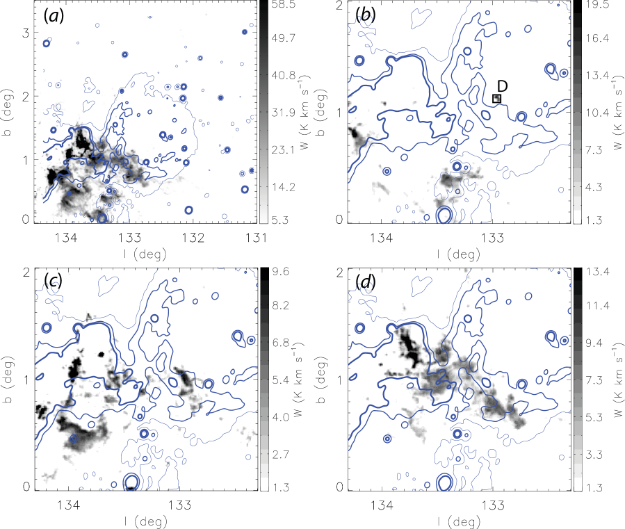
Figure 1: ¹²CO (J=1–0) emission maps integrated over four velocity ranges, (a) $-53$ to $-35$  km s^-1, (b) $-52$ to $-51$  km s^-1, (c) $-46$ to $-45$  km s^-1, and (d) $-42$ to $-41$  km s^-1. We show the integrated CO emission in the whole observed region in panel (a), and the representative channel maps (with the velocity width of 1  km s^-1and the RMS of $\sim$$0.21$ K) in the other panels. The minimum value of each map is $5\sigma$. The contours repeated on each panel are the CGPS radio continuum emission at 408 MHz, with the thicker lines indicating the higher intensities. The contour levels are 65, 87.5, and 110 K. The region that contains a binary clump is marked with a black box around ($l=132^{\circ}.94,b=1^{\circ}.12$) in panel (b), namely region D.

The ¹²CO intensity maps shown in Figure 1 exhibit the distribution of molecular gas around $-45$  km s^-1. There is substantial molecular gas associated with the nearby H ii complex, i.e. W3, ($l=133^{\circ}.8,b=1^{\circ}.2$; see Green, 2007), which is present in the whole velocity range of $-53$ to $-35$  km s^-1. There is also molecular gas in the remnant region, distributed along the radio continuum shell of the remnant. Based on their spatial and velocity continuities, we confirm that these molecular gases are from a same MC. In the middle of the conjunction area between W3 and HB 3, ¹²CO (J=1–0) emission protrudes from the W3 region into the HB 3 region. There is no strong CO emission detected in the north and northwest of the remnant. Kilpatrick et al. (2016) detected ¹²CO (J=2-1) emission toward two small regions ($10^{\prime}\times 30^{\prime}$ and $10^{\prime}\times 10^{\prime}$) in the far north of the remnant, however, they suggested that the detected broad molecular line region is associated with the W3 complex, but not the remnant. The distribution of molecular gas is morphologically consistent with the non-thermal radio continuum emission of the remnant, which shows blowout morphology from the north to northwest and bright shell from the east to southwest. It is somewhat similar to the blowout morphology in the SNR N132D (e.g., Dickel & Milne, 1995; Xiao & Chen, 2008), which was suggested to be shaped by the shock impacting on a stellar wind-bubble shell (Hughes, 1987; Chen et al., 2003). The radio continuum emissions of the remnant and the W3 complex are in conjunction with each other as well (around $l=133^{\circ}.2,b=1^{\circ}.0$), without a clear border between them. Along with the velocity component around -45 km s^-1, there are also the other velocity components, around 0  km s^-1, $-75$  km s^-1, and $-105$  km s^-1. We have checked them, and find no morphological correlations to the remnant.

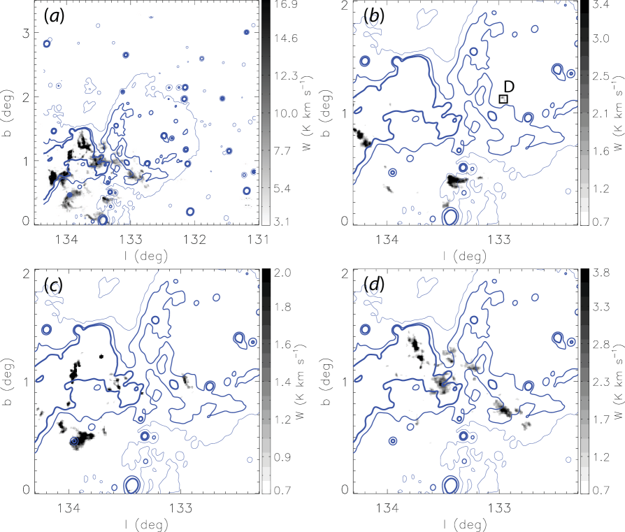
Figure 2: The same as Figure 1, but for ¹³CO (J=1–0) emission. The RMS of 1  km s^-1 channel map is $\sim$$0.12$ K.

Figure 2 shows the ¹³CO intensity maps produced in the same manner as Figure 1. The ¹³CO emission is less extended than ¹²CO, with the peak in the W3 region. We also detect some ¹³CO emissions along the radio shell of the remnant. There is no significant C¹⁸O emission detected in the remnant region.

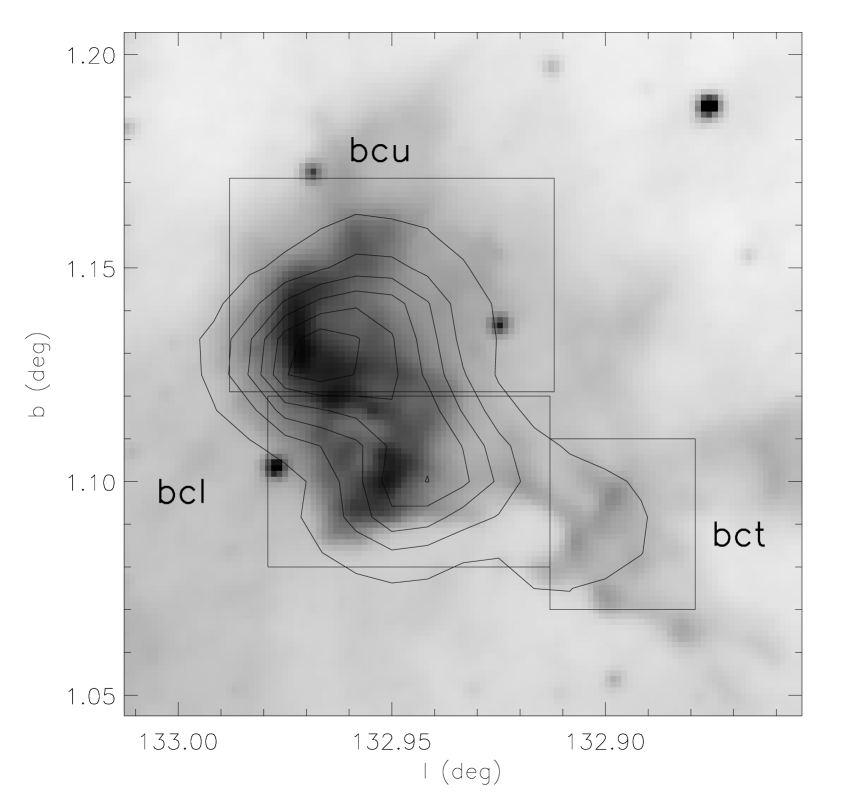
Figure 3: WISE 12 $\mu$m image of the binary clump overlaid with integrated intensity contours of ¹²CO (J=1–0) emission in the velocity range of $-53$ to $-49$  km s^-1. The contours have the minimum of $5\sigma$ with a step of $10\sigma$. The RMS is $\sim$0.42 K. The binary clump is divided into three regions, namely, the binary clump upper region, the binary clump lower region, and the binary clump tail region, which are indicated by rectangles labeled bcu, bcl, and bct, respectively.

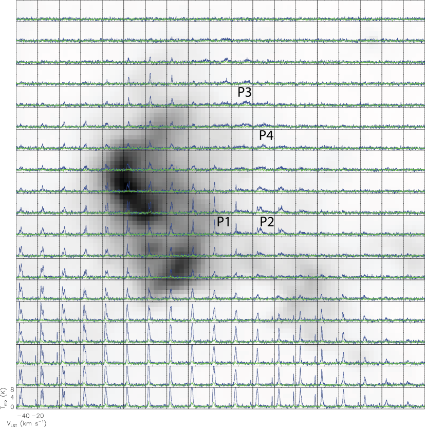
Figure 4: Grid of ¹²CO (J=1–0) (blue) and ¹³CO (J=1–0) (green) spectra around $-45$  km s^-1 in region D (see panel (b) in Figures 1 and 2), superposed on the WISE 22 $\mu$m image. The image covers the same region shown in Figure 3. The grid spacing is 30^′′, corresponding to the length of 0.28$d_{1.95}$ pc. Four representative points are selected for spectral analysis, and labeled with P1, P2, P3, and P4, respectively.

Particularly, a binary clump is found at ($l=132^{\circ}.94,b=1^{\circ}.12$) around $-51.5$  km s^-1 inside the remnant’s radio shell, which is prominent in both ¹²CO and ¹³CO emissions. This binary clump, denoted as region D, is indicated in panel (b) in Figures 1 and 2. The two clumps in the system have a small velocity shift of $\sim$0.3  km s^-1. This $-51.5$  km s^-1 binary clump has a tail extending toward the western region too (see Figure 3), which is a sign of interaction between the two clumps. In the same region, near the binary clump, there is also a small protrusion from the $-45$  km s^-1 MC located around the radio shell of the remnant into the inner region of the remnant (see panel (c) in Figure 1).

Significant mid-IR emissions (12 $\mu$m and 22 $\mu$m) are also detected in the south-eastern part in region D (see Figures 3 and 4). The mid-IR emission has two peaks similar to the $-51.5$  km s^-1 component, but with the position shifted to the $-45$  km s^-1 protrusion. In addition, the mid-IR emission has a tail structure corresponding to that of the $-51.5$  km s^-1 component, where no significant $-45$  km s^-1 emission present. There are also weak mid-IR emissions beyond the binary clump in the west, northwest, and north (see Figure 3), with associated ¹²CO (J=1–0) emission around $-45$  km s^-1 but not $-51.5$  km s^-1.

3.2 Dynamics

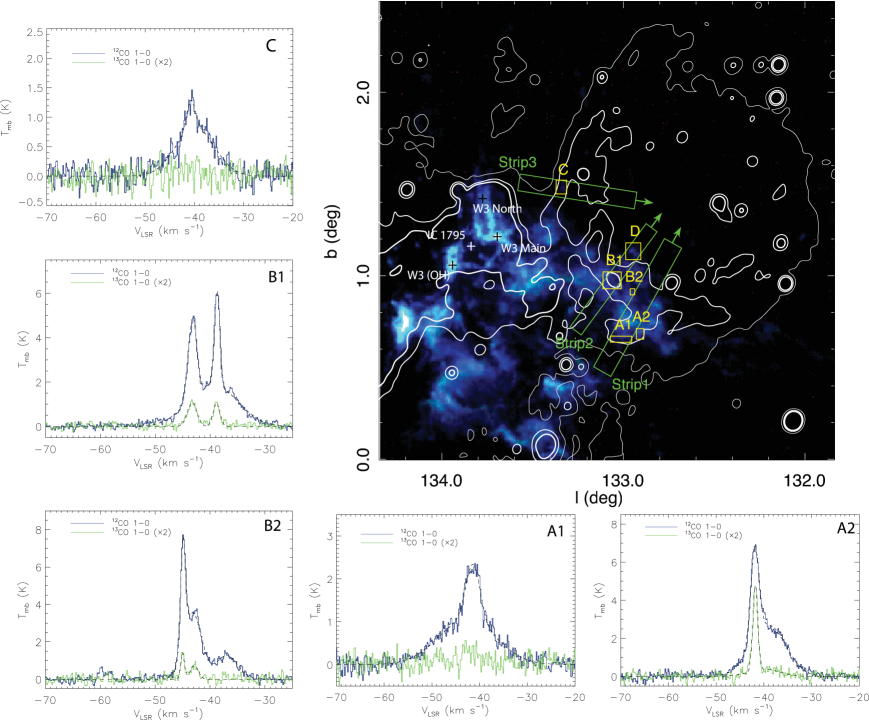
Figure 5: Right top panel: integrated intensity map of ¹²CO (J=1–0) emission (blue), ¹³CO (J=1–0) (green), and C¹⁸O (J=1–0) (red) in the velocity range of $-60$ to $-30$  km s^-1, overlaid with the same 408 MHz continuum contours as in Figure 1. The green and yellow regions are selected for generating position-velocity maps and for spectral analysis, respectively. Region D is the same as that in Figures 1 and 2. The prominent features of the W3 complex are labeled. Other five panels: the ¹²CO (J=1–0) (blue) and ¹³CO (J=1–0) (green) spectra extracted from the corresponding regions A1, A2, B1, B2, and C, respectively. The ¹³CO (J=1–0) spectra are multiplied by a factor of 2 for a better visibility. The spectra are fitted by multiple Gaussian components, with the fitting results shown by black dashed lines (see the fitted parameters in Table 1).

Table 1: Fitted parameters of thermal molecular lines.

region	component	Line	Peak $T_{\rm mb}$	Center $V_{\rm LSR}$	FWHM
			(K)	( km s-1)	( km s-1)
A1	narrow	12CO (J=1–0)	1.31$\pm{0.06}$	-41.38$\pm{0.06}$	3.5$\pm{0.2}$
		13CO (J=1–0)	$\leq{0.08}$	-	-
	broad	12CO (J=1–0)	1.05$\pm{0.05}$	-42.7$\pm{0.2}$	14.1$\pm{0.5}$
		13CO (J=1–0)	$\leq{0.08}$	-	-
A2	narrow	12CO (J=1–0)	4.83$\pm{0.08}$	-41.89$\pm{0.02}$	2.01$\pm{0.04}$
		13CO (J=1–0)	2.21$\pm{0.05}$	-41.79$\pm{0.02}$	1.22$\pm{0.04}$
	broad	12CO (J=1–0)	2.70$\pm{0.05}$	-39.10$\pm{0.07}$	8.7$\pm{0.2}$
		13CO (J=1–0)	0.19$\pm{0.1}$	-39.9$\pm{0.5}$	7.9$\pm{0.9}$
B1	narrow1	12CO (J=1–0)	3.56$\pm{0.06}$	-43.23$\pm{0.02}$	1.80$\pm{0.04}$
		13CO (J=1–0)	0.53$\pm{0.03}$	-43.29$\pm{0.05}$	2.1$\pm{0.1}$
	narrow2	12CO (J=1–0)	4.26$\pm{0.07}$	-38.744$\pm{0.009}$	1.13$\pm{0.03}$
		13CO (J=1–0)	0.52$\pm{0.03}$	-38.87$\pm{0.03}$	1.47$\pm{0.09}$
	broad	12CO (J=1–0)	1.89$\pm{0.04}$	-39.48$\pm{0.08}$	10.4$\pm{0.2}$
		13CO (J=1–0)	$\leq{0.05}$	-	-
B2	narrow1	12CO (J=1–0)	5.6$\pm{0.2}$	-44.92$\pm{0.01}$	1.02$\pm{0.03}$
		13CO (J=1–0)	0.71$\pm{0.06}$	-44.99$\pm{0.04}$	0.82$\pm{0.08}$
	narrow2	12CO (J=1–0)	3.54$\pm{0.06}$	-43.19$\pm{0.06}$	3.9$\pm{0.1}$
		13CO (J=1–0)	0.36$\pm{0.04}$	-42.9$\pm{0.1}$	1.7$\pm{0.3}$
	broad	12CO (J=1–0)	1.26$\pm{0.05}$	-37.0$\pm{0.1}$	4.7$\pm{0.3}$
		13CO (J=1–0)	$\leq{0.08}$	-	-
C	narrow	12CO (J=1–0)	0.47$\pm{0.07}$	-40.7$\pm{0.2}$	1.9$\pm{0.4}$
		13CO (J=1–0)	$\leq{0.08}$	-	-
	broad	12CO (J=1–0)	0.83$\pm{0.05}$	-39.9$\pm{0.2}$	9.3$\pm{0.5}$
		13CO (J=1–0)	$\leq{0.08}$	-	-

Broad ¹²CO (J=1–0) emission lines are detected in many places, and they have different velocities at different locations. In Figure 5, the spectra extracted from five selected regions are shown, namely A1, A2, B1, B2, and C. There are also broad ¹²CO (J=1–0) emission lines in region D (see Figure 4). These regions are distributed along the remnant’s radio shell around the conjunction area between the remnant and the W3 complex as well inside it. We do not find any evidence of association between these broad ¹²CO (J=1–0) emission-line regions and the H ii regions in the W3 complex. According to the correspondence of spatial distribution and as an exclusive source of disturbance, the broadened emission lines are originated from the molecular gas impacted by the remnant shock, which confirms the association between HB 3 and the MCs in the W3 complex. We have performed Gaussian fitting to the emission lines, and the fitted parameters are listed in Table 1. For most of the broad ¹²CO (J=1–0) components, the line centers are red-shifted comparing to the narrow components except in region A1. It indicates that the remnant is at the nearside of the MCs. Note that, in region C, both the narrow and broad components are weak, and the intensity of the broad component is stronger than that of the narrow component, indicating that there is not much quiet molecular gas left in this region.

Table 2: Fitted parameters of thermal molecular lines in region D.

region &point	component	Line	Peak $T_{\rm mb}$	Center $V_{\rm LSR}$	FWHM
			(K)	( km s-1)	( km s-1)
whole	narrow1	12CO (J=1–0)	5.45$\pm{0.06}$	-51.615$\pm{0.006}$	1.02$\pm{0.02}$
		13CO (J=1–0)	0.80$\pm{0.04}$	-51.81$\pm{0.02}$	0.84$\pm{0.05}$
	narrow2	12CO (J=1–0)	0.94$\pm{0.07}$	-45.17$\pm{0.04}$	0.89$\pm{0.09}$
		13CO (J=1–0)	0.16$\pm{0.05}$	-45.02$\pm{0.08}$	0.6$\pm{0.2}$
	narrow3	12CO (J=1–0)	1.78$\pm{0.04}$	-43.20$\pm{0.04}$	2.39$\pm{0.09}$
		13CO (J=1–0)	0.17$\pm{0.03}$	-43.2$\pm{0.2}$	2.0$\pm{0.4}$
	broad	12CO (J=1–0)	0.18$\pm{0.02}$	-36.6$\pm{0.9}$	20$\pm{2}$
		13CO (J=1–0)	$\leq{0.06}$	-	-
P1	narrow	12CO (J=1–0)	5.7$\pm{0.2}$	-43.29$\pm{0.02}$	1.16$\pm{0.05}$
		13CO (J=1–0)	0.66$\pm{0.10}$	-43.64$\pm{0.10}$	1.4$\pm{0.3}$
P2	narrow	12CO (J=1–0)	2.0$\pm{0.3}$	-43.46$\pm{0.05}$	0.9$\pm{0.2}$
		13CO (J=1–0)	$\leq{0.19}$	-	-
	broad	12CO (J=1–0)	2.13$\pm{0.08}$	-39.5$\pm{0.2}$	6.8$\pm{0.4}$
		13CO (J=1–0)	$\leq{0.19}$	-	-
P3	broad	12CO (J=1–0)	1.36$\pm{0.07}$	-29.7$\pm{0.3}$	11.3$\pm{0.7}$
		13CO (J=1–0)	$\leq{0.20}$	-	-
P4	broad	12CO (J=1–0)	1.14$\pm{0.07}$	-35.9$\pm{0.3}$	8.3$\pm{0.6}$
		13CO (J=1–0)	$\leq{0.20}$	-	-

We also detect broad ¹²CO (J=1–0) emission lines inside the bright radio shell of the remnant. Broad CO emission lines are detected in the north-western part in region D (see Figure 4). There are three narrow components in this region, around $-$51.5  km s^-1, $-$45  km s^-1, and $-$43  km s^-1 (see Table 2). The line center of broad component is around $-36$  km s^-1, which is far from the $-$51.5  km s^-1 component. Considering the velocity and position close to that of $-$43  km s^-1 MC, the broad component is associated to the $-$43  km s^-1 MC. Note that there is no broad component associated with the $-$51.5  km s^-1 component which corresponds to the binary molecular clump. We have not found any evidence of the binary clump being shocked by the remnant. We choose four representative points with a strong narrow emission line at $-$43  km s^-1 and broad emission lines at other three different velocities for spectral analysis, namely P1, P2, P3, and P4 (shown in Figure 4). By spectral analysis of the emission lines at these four points, the physical states of quiet and shocked molecular gases in region D are studied. The fitting results are listed in Table 2. In region D, the velocity shift of the broad component becomes larger as it goes further inside the projected extent of the remnant. At the positions of P3 and P4, we could not see the associated narrow component but only the broad components.

There is significant mid-IR emission (12 $\mu$m and 22 $\mu$m) in the south-eastern part of region D (see Section 3.1), which could be emitted by polycyclic aromatic hydrocarbon (PAH), hot dust, or both. The source of mid-IR emission is not clear. The morphology of mid-IR emission has two peaks similar as the $-51.5$  km s^-1 component, but with the position shifted to the $-45$  km s^-1 protrusion. Both the molecular shock in the $-45$  km s^-1 MC and the disturbed molecular gas in the $-51.5$  km s^-1 binary molecular clump may contribute to the mid-IR emission.

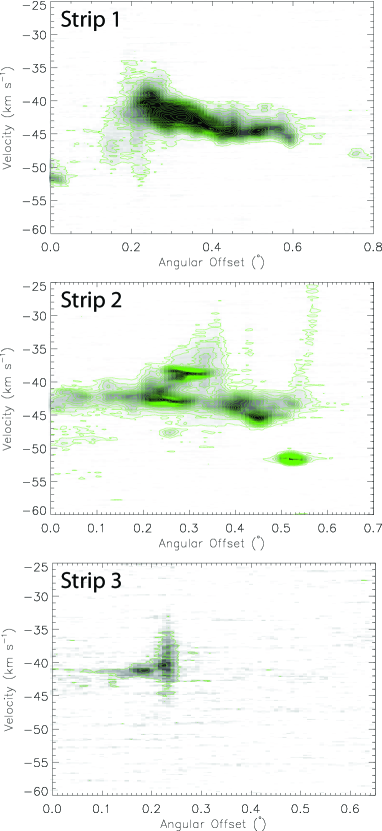
Figure 6: Position-velocity maps of ¹²CO (J=1–0) emission along the strips indicated by the green rectangular regions in Figure 5, with the directions indicated by the attached arrows. The contour levels are from $3\sigma$ and in a step of $1\sigma$. The RMS is $\sim$0.5 K.

In Figure 6, we present the position-velocity distributions of ¹²CO (J=1–0) emission along the strips indicated by the green rectangular regions shown in Figure 5, which are perpendicular to the radio continuum shell of the remnant. The broad CO wings are prominent and near the border of the remnant in strip 1 (region A1) and strip 3 (region C). In strip 1, the emission peak is inside the projected extent of the remnant, which could be due to the effect of line-of-sight superimposition. In strip 3, the intensity of broadened component is comparable to that of narrow component, and both are weak. It indicates that the amount of molecular gas in this region is not as large as in the other regions; nevertheless, the percentage of shocked molecular gas is higher than in the other regions.

In strip 2, the broad CO wings are presented at two positions, with the angular offsets of 0.35^∘ and 0.55^∘ (see Figure 6). One is at the radio peak (region B1), and the other is further inside the projected extent of the remnant (region D). Note that region B1 is in the middle of the conjunction area between W3 and HB 3, where CO emission protrudes from the W3 region into the HB 3 region. In this area, the radio continuum emission and the broad CO wings are intense, which indicates a strong interaction between the remnant and the MCs. Region D appears further inside the projected extent of the remnant than the other regions, and its broad component also has the largest line-width.

We confirm, based on both morphological and dynamical evidences, the association between the remnant and the $\sim$$-$45  km s^-1 MC, which is itself associated with the W3 H ii complex. Therefore, HB 3 is at the same distance as the W3/W4 complex, which is $1.95\pm 0.04$ kpc. Accordingly, the physical size of the remnant is $65\times 48$ pc².

4 Discussion

4.1 Physical Conditions of the Molecular Gas

Table 3: Derived physical parameters.

region	component	$T_{\rm ex}$	$\tau$(13CO)	$N({\rm H_{2}})$	$M$	$M_{\rm vir}$
		(K)		(1020 cm-2)	(${\rm M}_{\rm\odot}$)	(${\rm M}_{\rm\odot}$)
A1	narrow	$>$4.3	$<0.2$	$<9.7$ (8.8)	$<22{d}^{2}_{1.95}$ (63$d^{2}_{1.95}$)	5.1$\times 10^{3}$$d_{1.95}$
	broad	$>$4.0	$<0.3$	$<45$ (28)	$<1.1\times 10^{2}{d}^{2}_{1.95}$ (2.0$\times 10^{2}d^{2}_{1.95}$)	8.3$\times 10^{4}$$d_{1.95}$
A2	narrow	8.1	0.8	31 (19)	$1.2\times 10^{2}{d}^{2}_{1.95}$ ($84d^{2}_{1.95}$)	6.0$\times 10^{2}$$d_{1.95}$
	broad	$\geq$5.9	$\leq$0.3	51 (45)	59${d}^{2}_{1.95}$ (2.0$\times 10^{2}d^{2}_{1.95}$)	1.1$\times 10^{4}$$d_{1.95}$
B1	narrow1	6.8	0.3	18 (12)	1.6$\times 10^{2}{d}^{2}_{1.95}$ (2.1$\times 10^{2}d^{2}_{1.95}$)	1.2$\times 10^{3}$$d_{1.95}$
	narrow2	7.5	0.3	13 (9.2)	$1.0\times 10^{2}{d}^{2}_{1.95}$ (1.6$\times 10^{2}d^{2}_{1.95}$)	4.6$\times 10^{2}$$d_{1.95}$
	broad	$>$5.0	$<0.1$	$<18$(38)	$<79{d}^{2}_{1.95}$ (6.4$\times 10^{2}d^{2}_{1.95}$)	3.9$\times 10^{4}$$d_{1.95}$
B2	narrow1	8.9	0.3	9.3 (11)	7.2${d}^{2}_{1.95}$ (17$d^{2}_{1.95}$)	1.1$\times 10^{2}$$d_{1.95}$
	narrow2	6.8	0.4	15 (26)	8.0${d}^{2}_{1.95}$ (41$d^{2}_{1.95}$)	1.6$\times 10^{3}$$d_{1.95}$
	broad	$>$4.3	$<0.3$	$<18$(11)	$<6.8{d}^{2}_{1.95}$ (18$d^{2}_{1.95}$)	2.4$\times 10^{3}$$d_{1.95}$
C	narrow	$>$3.3	$<1.1$	$<21$ (1.7)	$<42{d}^{2}_{1.95}$ (14$d^{2}_{1.95}$)	9.7$\times 10^{2}$$d_{1.95}$
	broad	$>$3.8	$<0.5$	$<50$ (15)	$<1.0\times 10^{2}{d}^{2}_{1.95}$ (1.2$\times 10^{2}d^{2}_{1.95}$)	2.3$\times 10^{4}$$d_{1.95}$
Example points in region D
P1	narrow	9.0	0.1	6.8 (13)	0.9${d}^{2}_{1.95}$ (1.6$d^{2}_{1.95}$)	40$d_{1.95}$
P2	narrow	$>$5.1	$<0.5$	$<7.1$ (3.4)	$<0.2{d}^{2}_{1.95}$ (0.4$d^{2}_{1.95}$)	24$d_{1.95}$
	broad	$>$5.3	$<0.4$	$<51$ (28)	$<1.6{d}^{2}_{1.95}$ (3.6$d^{2}_{1.95}$)	1.4$\times 10^{3}$$d_{1.95}$
P3	broad	$>$4.4	$<0.9$	$<1.3\times 10^{2}$ (29)	$<4.3{d}^{2}_{1.95}$ (3.8$d^{2}_{1.95}$)	3.8$\times 10^{3}$$d_{1.95}$
P4	broad	$>$4.1	$<1.2$	$<1.2\times 10^{2}$ (18)	$<4.0{d}^{2}_{1.95}$ (2.3$d^{2}_{1.95}$)	2.1$\times 10^{3}$$d_{1.95}$

We estimate the physical parameters of molecular gas in the selected regions. For ¹²CO (J=1–0), given the background temperature ${T}_{\rm bg}=2.73$ K, we get the excitation temperature as:

$$T_{\rm ex}=5.53({\rm log}(1+\frac{5.53}{T_{\rm mb,peak,^{12}CO}/(1-{\rm exp}(-\tau_{\rm{}^{12}CO}))+0.84}))^{-1}~{}({\rm K}),$$ (1)

where $\tau$ and ${T}_{\rm mb,peak}$ are the optical depth and the peak ${T}_{\rm mb}$ of the corresponding emission lines, respectively. In the assumption of local thermodynamic equilibrium (LTE), the excitation temperatures of ¹²CO (J=1–0) and ¹³CO (J=1–0) should be the same; we could derive the optical depth of ¹³CO (J=1–0) as:

$$\tau_{\rm{}^{13}CO}=-{\rm log}(1-\frac{T_{\rm mb,peak,^{13}CO}/f_{\rm{}^{13}CO}}{5.29(\frac{1}{{\rm exp}(5.29/T_{\rm ex})}-0.17)}),$$ (2)

and the column density of ¹³CO as (e.g. Garden et al., 1991):

$$\begin{split}N_{\rm{}^{13}CO}&=2.50\times 10^{14}\frac{T_{\rm ex}+0.88}{1-{\rm exp}(-5.29/T_{\rm ex})}\int\tau_{\rm{}^{13}CO}dv~{}({\rm cm}^{-2})\\ &\simeq 2.50\times 10^{14}\frac{T_{\rm ex}+0.88}{1-{\rm exp}(-5.29/T_{\rm ex})}\tau_{\rm{}^{13}CO}\Delta v_{\rm{}^{13}CO},\end{split}$$ (3)

where $f_{\rm{}^{13}{CO}}$ and $\Delta v_{\rm{}^{13}{CO}}$ are the area beam-filling factor and the full width at half maximum (FWHM) of ¹³CO (J=1–0), respectively. The area beam-filling factor of ¹²CO (J=1–0) is assumed to be unity in our calculation, which is reasonable considering that the selected regions are filled with ¹²CO (J=1–0) emission. However, ¹³CO (J=1–0) is not in this case, and its area beam-filling factor is estimated by the ratio of the number of points with detected ¹³CO emission to that with detected ¹²CO emission. For the regions without detected ¹³CO (J=1–0), the area beam-filling factor of ¹³CO is assumed to be the minimum one of that from the regions with detected ¹³CO (J=1–0), which is $1/4$.

Applying $\tau_{\rm{}^{12}CO}/\tau_{\rm{}^{13}CO}\simeq N_{\rm{}^{12}CO}/N_{\rm{}^{13}CO}\simeq[^{12}{\rm C}/^{13}{\rm C}]=70$ (Milam et al., 2005) to Equation (1) and Equation (2), we calculated the $T_{\rm ex}$ and $\tau_{\rm{}^{13}CO}$ recursively. The derived physical parameters are listed in Table 3. For the MC with a low column density, the photodissociation rates can be different for ¹²CO and ¹³CO, which may cause $N_{\rm{}^{12}CO}/N_{\rm{}^{13}CO}\gtrsim[^{12}{\rm C}/^{13}{\rm C}]$. But this effect only causes an increase of the ratio up to 25 percent (Szűcs et al., 2014).

Most of the broad components do not have corresponding ¹³CO (J=1–0) emission detected, which indicates that their ¹²CO (J=1–0) emissions are optically thin. Therefore, the excitation temperature of these broad components cannot be well determined. We detect broad ¹³CO (J=1–0) emission in region A2, and the ratio of brightness temperatures $f_{\rm{}^{13}CO}\times T_{\rm mb,peak,^{12}CO}/T_{\rm mb,peak,^{13}CO}$ are $4\pm 2$ for the broad component and $1.88\pm 0.02$ for the narrow component. Considering the possibility of this broad ¹²CO (J=1–0) emission being optically thin too, we give the derived excitation temperature as a lower limit in region A2 either. Note that, the large velocity widths of the lines support high excitation temperature.

The stability of MC could be investigated by the virial theorem. The mass of all the molecular clouds is smaller than their virial mass (see Table 3). However, it can be caused by the small sizes of the selected regions, which are about one order of magnitude smaller than the size of the target clouds. Taking this into account, the narrow components should be stable, with gravity and disturbance in equilibrium. Since the broad components are mainly distributed in small regions, no correction for size is needed. The mass of the broad components is at least two orders of magnitude lower than their virial mass, which indicates the existence of strong perturbations in these regions.

4.2 Properties of SNR HB 3

Adopted from the radio continuum extent of the remnant ($\sim 90^{\prime}$, see Figure 5), the radius of the remnant is $r_{\rm s}\sim 25.5$$d_{1.95}$ pc. Assuming the remnant is in the Sedov phase, and applying the velocity of the remnant’s shock $v_{\rm s}=340\pm{37}$  km s^-1 and the remnant’s ambient particle density $n_{\rm 0}=0.32\pm 0.10$  cm^-3 (derived from the X-ray study by Lazendic & Slane, 2006), we get the age of the remnant as $t\sim(2.9\pm{0.3})\times 10^{4}$$d_{1.95}$ yr, and the explosion energy as $E\sim(1.3\pm{0.8})\times 10^{51}{d}_{1.95}^{3}$ erg. Alternatively, the remnant may already enter the radiative phase. In this case, the age of the remnant is $t=(2r_{\rm s})/(7v_{\rm s})\sim(2.1\pm{0.2})\times 10^{4}$$d_{1.95}$ yr (McKee & Ostriker, 1977), and the explosion energy is $E=6.8\times 10^{43}n_{\rm 0}^{1.16}(\frac{v_{\rm s}}{1~{}{\rm km}~{}{\rm s}^{-1}})^{1.35}(\frac{r_{\rm s}}{1~{}{\rm pc}})^{3.16}\zeta_{\rm m}^{0.161}$ $\sim(1.6\pm{0.9})\times 10^{51}{d}_{1.95}^{3.16}$ erg, where $\zeta_{\rm m}=Z/Z_{\rm\odot}=1$ (Cioffi et al., 1988). The derived energies have large errors; however, they are basically consistent in the two cases.

We adopt the same velocity of the remnant’s shock and ambient particle density as that in Lazendic & Slane (2006). Nevertheless, we use a revised distance of 1.95 kpc, which is smaller than that of 2.2 kpc used in Lazendic & Slane (2006). Therefore, in the case of the Sedov phase, we get the age of the remnant very similar to that from Lazendic & Slane (2006), and get the explosion energy more different, since the age is proportional to the distance, whereas the explosion energy is proportional to the 3rd power of the distance.

HB 3 is surrounded by a partial molecular shell from the east to the southwest (see panel (a) in Figure 1 and Figure 5). This partial molecular shell could be swept up by either the SNR or the stellar wind of the SNR’s progenitor. If it was swept up by the progenitor’s stellar wind, the progenitor’s mass could be estimated by using the linear relationship between the size of the wind-blown bubble in a molecular environment and the star’s initial mass (Chen et al., 2013). The radius of the wind-blown bubble is no less than the radius of the partial molecular shell, which is $\gtrsim$$25$ pc. Then the mass of HB 3’s progenitor is $\gtrsim$$28~{}{\rm M}_{\rm\odot}$.

4.3 Binary molecular clump

Table 4: Fitted and derived parameters of thermal molecular lines from the binary molecular clump.

region	Line	Peak $T_{\rm mb}$	Center $V_{\rm LSR}$	FWHM
		(K)	( km s-1)	( km s-1)
bcu	12CO (J=1–0)	7.85$\pm{0.08}$	-51.704$\pm{0.005}$	0.96$\pm{0.01}$
	13CO (J=1–0)	1.28$\pm{0.05}$	-51.89$\pm{0.02}$	0.81$\pm{0.03}$
bcl	12CO (J=1–0)	5.95$\pm{0.07}$	-51.411$\pm{0.006}$	1.03$\pm{0.02}$
	13CO (J=1–0)	0.73$\pm{0.05}$	-51.58$\pm{0.03}$	0.68$\pm{0.06}$
bct	12CO (J=1–0)	1.88$\pm{0.07}$	-50.73$\pm{0.02}$	1.12$\pm{0.05}$
	13CO (J=1–0)	0$\pm{0.07}$	-	-
Derived parameters
region	$T_{\rm ex}$	$\tau$(13CO)	$N({\rm H_{2}})$	$M$	$M_{\rm vir}$
	(K)		(1020 cm-2)	(${\rm M}_{\rm\odot}$)	(${\rm M}_{\rm\odot}$)
bcu	11.2	0.2	11 (14)	59${d}^{2}_{1.95}$ ($1.0\times 10^{2}d^{2}_{1.95}$)	2.5$\times 10^{2}$$d_{1.95}$
bcl	9.3	0.2	5.6 (12)	16${d}^{2}_{1.95}$ (48$d^{2}_{1.95}$)	2.5$\times 10^{2}$$d_{1.95}$
bct	$>$5.0	$<$0.2	$<$2.9 (4.0)	$<$1.8${d}^{2}_{1.95}$ (10$d^{2}_{1.95}$)	1.9$\times 10^{2}$$d_{1.95}$

We investigate the physical state of the binary molecular clump by analyzing its CO emission lines. The CO spectra are extracted from three regions of the binary clump, namely, bcu, bcl, and bct, corresponding to the upper clump, the lower clump, and the tail of the binary clump, respectively (see Figure 3). Using the same method as in Section 4.1, we estimate the physical parameters of the molecular gas in these regions. The fitted and derived parameters of the CO emission lines are listed in Table 4.

The mass of the upper clump is smaller than its virial mass (the virial parameter $\alpha_{\rm vir,bcu}=M_{\rm vir,bcu}/M_{\rm bcu}\sim 4$). However, the factor is only a few, indicating that the upper clump is about stable. For the lower clump, the mass is about one order of magnitude smaller than its virial mass ($\alpha_{\rm vir,bcl}\sim 16$). Therefore, the lower clump is significantly disturbed. The virial parameter of the tail is $\alpha_{\rm vir,bct}\gtrsim 1\times 10^{2}$, implying that the tail is loosely bound by the system.

The clumps in a binary system are affected by tidal force, which could destroy these clumps. To estimate the effect of tidal force on the upper clump, we derive the ratio between the tidal force and the self-gravity as $\gamma_{\rm bcu}\sim 4M_{\rm bcl}M_{\rm bcu}^{-1}rr_{\rm bcu}^{3}(r^{2}-r_{\rm bcu}^{2})^{-2}$ $\sim 0.82(1.90~{}{\rm sin}^{-1.5}\theta-0.67~{}{\rm sin}^{0.5}\theta)^{-2}$ $\lesssim 0.54$, where $M_{\rm bcl}$ and $M_{\rm bcu}$ are the mass of the lower and upper clumps, respectively, $r$ is the distance between the two clumps, and $r_{\rm bcu}$ is the radius of the upper clump. For the lower clump, we get the tidal force factor $\gamma_{\rm bcl}\lesssim 1.38$. Therefore, the tidal force could not directly destroy the upper clump in the binary system, but could destroy the lower clump. In any case, the tidal disturbance will play an important role during the evolution of the binary system. The tail structure here in the binary system resembles the tidal tails of interacting galaxies, e.g. NGC 3256 and NGC 5752/4 (Keel & Borne, 2003; Trancho et al., 2007; Smith et al., 2010), etc. The loosely bound tail material could get stripped during the interaction process. The angular momentum would be taken away, and hence the binary system becomes stable. Such molecular clump interaction may induce star-formations; nevertheless, the clumps could be stripped and lose their mass.

4.4 Star Formation Activity

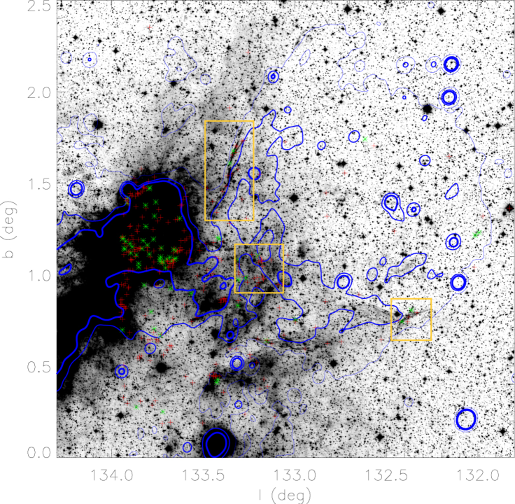
Figure 7: Image of 4.6 $\mu$m emission observed by WISE, overlaid with the same 408 MHz continuum contours as in Figure 1 (in blue). The positions of young stellar object candidates (YSOc) are marked with green stars (type Class I) and red pluses (type Class II). Aggregated YSOc in the HB 3 region are divided into three clusters, which are marked with yellow rectangular boxes in the east, southeast, and southwest of the remnant.

We have selected young stellar object candidates (YSOc) from the IR data (see Figure 7). Using the color-color and WISE photometry criteria described in Koenig et al. (2012), disk-bearing young stars are identified, of which the IR colors are distinctly different from those of diskless objects. Diskless young stars cannot be distinguished from unrelated field objects based on IR colors alone. For the sources that are not detected in the WISE [12] band, the $K_{\rm s}$$-$[3.4] versus [3.4]$-$[4.6] color–color diagrams are constructed based on their dereddened photometry in the WISE [3.4] and [4.6] bands, in combination with the dereddened 2MASS $K_{\rm s}$ photometry. To deredden the photometry, we estimate the extinction by the locations in the $J$$-$$H$ versus $H$$-$$K_{\rm s}$ color–color diagram (see details in Fang et al., 2013). We have further checked the YSOc by eye to exclude the sources that are not point-like, to maximally eliminate the contamination from small shocked clumps.

The YSOc are mainly distributed within the W3 region, and also in the conjunction area between W3 and HB 3 (see Figure 7). Most of YSOc in the HB 3 region are aggregated and along the outer rim of the radio shell of HB 3. We could generally divide them into three clusters. The most distinctive one is in the east of the remnant, which is spatially corresponding not only with 4.6 $\mu$m filaments but also with the eastern edge of HB 3 where radio emission is the most steep (see Figure 7). In this region, we detect weak CO emissions, with line wing broadening features. Another cluster is in the southwest of the remnant, around the top-end of the remnant’s radio shell, where the border of radio continuum emission is a little dent. It is also associated with a shorter curved 4.6 $\mu$m filament. The rests of aggregated YSOc are in the southeast of the remnant, around the conjunction point between the remnant and the W3 region, where both the radio continuum emission and the ¹²CO (J=1–0) emission are strong. The distribution of aggregated YSOc shows very well morphological correlations with the radio emission of HB 3. It provides a strong evidence of association between the SNR and the underlying star-formation activities, which indicates the ignition of star-formation at the periphery of a well-developed star-forming region. Due to the short lifetime of the remnant, the related star-formation activities are hardly being triggered by HB 3 directly, but are probably triggered by the stellar wind of HB 3’s progenitor. It indicates that the partial molecular shell surrounding the remnant from the east to the southwest was swept up by the progenitor’s stellar wind. Therefore, the mass of HB 3’s progenitor is $\gtrsim$$28~{}{\rm M}_{\rm\odot}$ (see Section 4.2).

Oey et al. (2005) suggested that W3/W4 was a three-generation hierarchical star-forming system. The current star-forming activities in W3 could be triggered by the OB association IC 1795. The age of IC 1795 is 3 to 5 Myr (Oey et al., 2005), which could belong to the same generation as HB 3’s progenitor. The distance between HB 3’s geometrical center and IC 1795 is about 41$d_{1.95}$ pc. If HB 3’s progenitor were a runaway star from IC 1795, its velocity would be about 8 to 13$d_{1.95}$  km s^-1 that is moderate (e.g. Banerjee et al., 2012). Indeed, the O- and B-type stars are widely dispersed across the W3 complex (Kiminki et al., 2015). It is possible that HB 3’s progenitor used to be in IC 1795. This suggests that the propagation of star-formation could be very fast, and the case of the next generation triggered star-formation could be truly complicated.

5 Conclusions

We present millimeter observations in CO emission lines toward HB 3. Substantial molecular gas around $-45$  km s^-1 is detected in the conjunction region between the SNR HB 3 and the nearby H ii region/MC complex W3. This molecular gas is distributed along the radio continuum shell of the remnant. Furthermore, the shocked molecular gas indicated by line wing broadening features is also distributed along the radio shell and inside it. By both morphological correspondence and dynamical evidence, we confirm that the SNR HB 3 is interacting with the $-45$  km s^-1 MC, in essence, with the nearby H ii region/MC complex W3. The red-shifted line wing broadening features indicate that the remnant is at the nearside of the MC. With this association, we could place the remnant at the same distance as the W3/W4 complex, which is $1.95\pm 0.04$ kpc. We also find a spatial correlation between the aggregated YSOc and the shocked molecular strip which is associated with the remnant.

Particularly, a binary clump at ($l=132^{\circ}.94,b=1^{\circ}.12$) around $-51.5$  km s^-1 inside the remnant’s radio shell has been found, and it is associated with significant mid-IR emission. The binary system also has a tail structure resembling the tidal tails of interacting galaxies. According to the analysis of CO emission lines, the larger clump in this binary system is approaching stability, and the smaller clump is significantly disturbed.

References

- Banerjee et al. (2012) Banerjee, S., Kroupa, P., & Oh, S. 2012, ApJ, 746, 15
- Caswell (1967) Caswell, J. L. 1967, MNRAS, 136, 11
- Chen et al. (2003) Chen, Y., Zhang, F., Williams, R. M., & Wang, Q. D. 2003, ApJ, 595, 227
- Chen et al. (2013) Chen, Y., Zhou, P., & Chu, Y.-H. 2013, ApJ, 769, L16
- Cioffi et al. (1988) Cioffi, D. F., McKee, C. F., & Bertschinger, E. 1988, ApJ, 334, 252
- Dame et al. (2001) Dame, T. M., Hartmann, D., & Thaddeus, P. 2001, ApJ, 547, 792
- Dickel & Milne (1995) Dickel, J. R., & Milne, D. K. 1995, AJ, 109, 200
- Fang et al. (2013) Fang, M., Kim, J. S., van Boekel, R., et al. 2013, ApJS, 207, 5
- Fesen et al. (1995) Fesen, R. A., Downes, R. A., Wallace, D., & Normandeau, M. 1995, AJ, 110, 2876
- Garden et al. (1991) Garden, R. P., Hayashi, M., Hasegawa, T., Gatley, I., & Kaifu, N. 1991, ApJ, 374, 540
- Green (2007) Green, D. A. 2007, Bulletin of the Astronomical Society of India, 35, 77
- Hanbury Brown & Hazard (1953) Hanbury Brown, R., & Hazard, C. 1953, MNRAS, 113, 123
- Hughes (1987) Hughes, J. P. 1987, ApJ, 314, 103
- Keel & Borne (2003) Keel, W. C., & Borne, K. D. 2003, AJ, 126, 1257
- Kilpatrick et al. (2016) Kilpatrick, C. D., Bieging, J. H., & Rieke, G. H. 2016, ApJ, 816, 1
- Kiminki et al. (2015) Kiminki, M. M., Kim, J. S., Bagley, M. B., Sherry, W. H., & Rieke, G. H. 2015, ApJ, 813, 42
- Koenig et al. (2012) Koenig, X. P., Leisawitz, D. T., Benford, D. J., et al. 2012, ApJ, 744, 130
- Koralesky et al. (1998) Koralesky, B., Frail, D. A., Goss, W. M., Claussen, M. J., & Green, A. J. 1998, AJ, 116, 1323
- Landecker et al. (1987) Landecker, T. L., Dewdney, P. E., Vaneldik, J. F., & Routledge, D. 1987, AJ, 94, 111
- Lazendic & Slane (2006) Lazendic, J. S., & Slane, P. O. 2006, ApJ, 647, 350
- MacLaren et al. (1988) MacLaren, I., Richardson, K. M., & Wolfendale, A. W. 1988, ApJ, 333, 821
- McKee & Ostriker (1977) McKee, C. F., & Ostriker, J. P. 1977, ApJ, 218, 148
- Milam et al. (2005) Milam, S. N., Savage, C., Brewster, M. A., Ziurys, L. M., & Wyckoff, S. 2005, ApJ, 634, 1126
- Normandeau et al. (1997) Normandeau, M., Taylor, A. R., & Dewdney, P. E. 1997, ApJS, 108, 279
- Oey et al. (2005) Oey, M. S., Watson, A. M., Kern, K., & Walth, G. L. 2005, AJ, 129, 393
- Reich et al. (2003) Reich, W., Zhang, X., & Fürst, E. 2003, A&A, 408, 961
- Ripple et al. (2013) Ripple, F., Heyer, M. H., Gutermuth, R., Snell, R. L., & Brunt, C. M. 2013, MNRAS, 431, 1296
- Routledge et al. (1991) Routledge, D., Dewdney, P. E., Landecker, T. L., & Vaneldik, J. F. 1991, A&A, 247, 529
- Shan et al. (2012) Shan, W. L., Yang, J., Shi, S. C., et al. 2012, IEEE Transactions on Terahertz Science and Technology, 2, 593
- Skrutskie et al. (2006) Skrutskie, M. F., Cutri, R. M., Stiening, R., et al. 2006, AJ, 131, 1163
- Smith et al. (2010) Smith, B. J., Giroux, M. L., Struck, C., & Hancock, M. 2010, AJ, 139, 1212
- Szűcs et al. (2014) Szűcs, L., Glover, S. C. O., & Klessen, R. S. 2014, MNRAS, 445, 4055
- Taylor et al. (2003) Taylor, A. R., Gibson, S. J., Peracaula, M., et al. 2003, AJ, 125, 3145
- Tian & Leahy (2005) Tian, W. W., & Leahy, D. 2005, A&A, 436, 187
- Trancho et al. (2007) Trancho, G., Bastian, N., Schweizer, F., & Miller, B. W. 2007, ApJ, 658, 993
- Ulich & Haas (1976) Ulich, B. L., & Haas, R. W. 1976, ApJS, 30, 247
- Williams et al. (1966) Williams, P. J. S., Kenderdine, S., & Baldwin, J. E. 1966, MmRAS, 70, 53
- Wright et al. (2010) Wright, E. L., Eisenhardt, P. R. M., Mainzer, A. K., et al. 2010, AJ, 140, 1868
- Xiao & Chen (2008) Xiao, X., & Chen, Y. 2008, Advances in Space Research, 41, 416
- Xu et al. (2006) Xu, Y., Reid, M. J., Zheng, X. W., & Menten, K. M. 2006, Science, 311, 54
- Zuo et al. (2011) Zuo, Y. X., Li, Y., Sun, J. X., et al. 2011, Acta Astronomica Sinica, 52, 152