Effects of Herzberg–Teller vibronic coupling on coherent excitation energy transfer

Abstract

In this work, we study the effects of non-Condon vibronic coupling on the quantum coherence of excitation energy transfer, via the exact dissipaton-equation-of-motion (DEOM) evaluations on excitonic model systems. Field-triggered excitation energy transfer dynamics and two dimensional coherent spectroscopy are simulated for both Condon and non-Condon vibronic couplings. Our results clearly demonstrate that the non-Condon vibronic coupling intensifies the dynamical electronic-vibrational energy transfer and enhances the total system-and-bath quantum coherence. Moreover, the hybrid bath dynamics for non-Condon effects enriches the theoretical calculation, and further sheds light on the interpretation of the experimental nonlinear spectroscopy.

I Introduction

The long-lived quantum beats in the coherent excitation energy transfer (EET) in biological light-harvesting systems have drawn plentiful attention in the past decade.Eng07782 ; Che084254 ; Pan1012766 ; Ple13235102 Two dimensional (2D) spectroscopy studies indicate that both electronic and vibrational coherence and their entanglement are responsible for this phenomenon. Tur111904 ; Tem1412865 ; But14034306 ; Cam1595 ; Bal1519491 This interpretation is confirmed by many theoretical works in the framework of the Franck–Condon approximation.Man121497 ; Per14404 ; Fuj15212403 ; Mon15065101 In the meanwhile, however, the non-Condon vibronic coupling is also proposed to enhance the quantum coherence in many organic and biological molecular systems.Ish082219 ; Kam0010637 ; Wom12154016 To obtain a better understanding of the origin of quantum coherence in EET dynamics, the interplay of the Condon and non-Condon vibronic coupling effects deserves more theoretical investigations.

In studying the vibronic coupling effects, we need an integrated theory to handle both the excitonic system and the vibrational environment. On the other hand, the nonlinear nature of 2D spectroscopy calls for non-perturbative and non-Markovian treatments, based on such as the hierarchical equations of motion (HEOM) approach.Tan89101 ; Yan04216 ; Ish053131 ; Tan06082001 ; Tan14044114 ; Tan15144110 ; Xu05041103 ; Xu07031107 ; Zhe121129 ; Jin08234703 ; Che11194508 However, HEOM focuses primarily on the reduced system only, despite it involves a vast number of auxiliary density operators, which are purely mathematical quantities. As an alternative exact approach for open systems, the recently developed dissipaton equation of motion (DEOM) theory Yan14054105 ; Zha15024112 ; Jin15234108 provides a quasi-particle dissipaton picture for the hybrid bath, and identifies its dynamical quantities as multi-body dissipaton density operators. In this manner, the DEOM is capable of treating both system and hybrid bath dynamics non-perturbatively. On describing reduced system dynamics, the DEOM recovers the HEOM method.Tan89101 ; Yan04216 ; Ish053131 ; Tan06082001 ; Tan14044114 ; Tan15144110 ; Xu05041103 ; Xu07031107 ; Zhe121129 ; Jin08234703 ; Che11194508 The optimized DEOM formalism with damped Brownian oscillators can be constructed for studying the system dynamics under the influence of solvent fluctuations and intramolecular vibrations.Xu09214111 ; Zhu115678 ; Din11164107 ; Din12224103 The DEOM further enables us to directly investigate the solvation bath dynamics. In fact, it has been successfully applied in studying a variety of Fano-type interferences,Zha15024112 ; Zha15214112 ; Xu151816 quantum transport current shot noise spectrum,Jin15234108 and solvent-induced non-Condon polarization effects.Zha16CP

In this work, we study the influence of non-Condon vibronic coupling on the coherent EET dynamics in excitonic model systems and compare it with the Condon counterpart, via the DEOM approach. In simulating the electronic excitation of the system, the vibrational coordinates are explicitly involved in the transition dipole moments. This accounts for the non-Condon vibronic coupling under the Herzberg-Teller approximation. Orl734513 ; Lin743802 ; Tan932263 ; Tan93118 ; Ish082219 We model these vibrational modes in terms of underdamped Brownian oscillators (BOs).Tho012991 ; Zhu115678 ; Din12224103 The underlying non-Condon effects are therefore studied via the hybrid bath dynamics in the DEOM framework.Zha16CP In the Franck–Condon approximation, however, the transition dipole moments are independent of nuclear coordinates and the underdamped BOs merely serve as the vibrational environment. Based on our simulations on field-triggered EET dynamics and coherent 2D spectroscopy, we conclude that the non-Condon vibronic coupling facilitates the dynamical electronic-vibrational energy transfer and enhances the total system-and-bath quantum coherence, at both cryogenic and room temperatures. While both the Condon and non-Condon vibronic coupling elongate the quantum beats, the non-Condon polarization improves the quantum yield of the excitonic system.

This paper is organized as follows. In Sec. II, we first set up an excitonic multi-chromophore system and model its surrounding environment with multiple Brownian oscillators, then briefly review the DEOM method and exemplify its application on the hybrid bath dynamics for non-Condon polarization effects. In Sec. III, we present the simulation results of field-triggered EET dynamics and coherent 2D spectroscopy for excitonic dimer systems, and compare the non-Condon and Condon vibronic coupling effects. The temperature dependence of these two effects is also discussed. Finally, we conclude this work in Sec. IV.

Throughout this paper, we set $\hbar=1$ and $\beta=1/(k_{B}T)$, with $k_{B}$ and $T$ being the Boltzmann constant and temperature, respectively.

II Methodology

II.1 Model Setup

Consider an excitonic multi-chromophore system embedded in an equilibrated thermal bath. The total composite system-and-bath Hamiltonian is summarized as $H_{\mbox{\tiny T}}=H_{\mbox{\tiny S}}+H_{\mbox{\tiny SB}}+h_{\mbox{\tiny B}}$. The excitonic system Hamiltonian reads

$$H_{\mbox{\tiny S}}=\epsilon_{g}|g\rangle\langle g|+\sum_{a}\epsilon_{a}|a\rangle\langle a|+\sum_{a\neq b}V_{ab}|a\rangle\langle b|.$$ (1)

Here, the ground state energy $\epsilon_{g}$ is often set to be zero, whereas the diagonal onsite energies and inter-site couplings denote $\{\epsilon_{a}\}$ and $\{V_{ab}\}$. The electronic dipole moment of each chromophore is $\hat{\mu}_{a}=\mu_{a}({\bf X}_{a})(|g\rangle\langle a|+|a\rangle\langle g|)$, where the transition matrix element $\mu_{a}({\bf X}_{a})$ depends on the nuclear coordinates ${\bf X}_{a}$. This form in fact accounts for the non-Condon coupling under the Herzberg–Teller approximation.Lin743802 In the Franck–Condon limit, $\mu_{a}({\bf X}_{a})$ becomes a constant without dependence on ${\bf X}_{a}$.

The thermal bath is modeled as numerous harmonic oscillators, $h_{\mbox{\tiny B}}=\sum_{j}\omega_{j}(p_{j}^{2}+x_{j}^{2})/2$, and the system-bath coupling takes the factorization form, i.e.,

$$H_{\mbox{\tiny SB}}=\sum_{a}\hat{Q}_{a}\hat{F}_{a},$$ (2)

where $\hat{Q}_{a}=|a\rangle\langle a|$ is a system operator and $\hat{F}_{a}=\sum_{j}c_{aj}x_{j}$ is a linear collective bath operator. The bath influence on the reduced system can be entirely characterized by the hybrid bath spectral density $J_{ab}(\omega)=\frac{\pi}{2}\sum_{j}c_{aj}^{2}\delta(\omega-\omega_{j})$, or the macroscopic bare-bath correlation function (setting $t>0$ hereafter),

$$\langle\hat{F}_{a}(t)\hat{F}_{b}(0)\rangle_{\mbox{\tiny B}}=\frac{1}{\pi}\int_{-\infty}^{\infty}\!d\omega\,\frac{e^{-i\omega t}J_{ab}(\omega)}{1-e^{-\beta\omega}}\approx\sum_{k}\eta_{abk}e^{-\gamma_{k}t},$$ (3)

with $\hat{F}_{a}(t)=e^{ih_{\mbox{\tiny B}}t}\hat{F}_{a}e^{-ih_{\mbox{\tiny B}}t}$ being a Gaussian stochastic variable in the $h_{\mbox{\tiny B}}$-interaction picture. The first identity is the fluctuation–dissipation theorem, Wei08 ; Yan05187 while the second involves the parameterization of $J_{ab}(\omega)$ and certain sum-over-pole expansion of Bose function, $f^{\rm Bose}(\omega)=(1-e^{-\beta\omega})^{-1}$, followed by the Cauchy contour integral. The time-reversal correspondence to Eq. (3) reads

$$\langle\hat{F}_{b}(0)\hat{F}_{a}(t)\rangle_{\mbox{\tiny B}}=\sum_{k}\eta_{ab\bar{k}}^{\ast}e^{-\gamma_{k}t}.$$ (4)

The second expression, where the associate index $\bar{k}$ goes with $\gamma_{\bar{k}}=\gamma_{k}^{\ast}$, reflects the fact that $\gamma_{k}$ and $\gamma_{k}^{\ast}$ must both appear if they are complex. Apparently, $\bar{k}=k$ for a real $\gamma_{k}$.

For the bath spectral density, we adopt the multiple Brownian oscillators (BOs) model. It can describe optically active vibronic coupling via the underdamped BO mode and also energy fluctuation via strongly overdamped Drude dissipation. For simplicity, we omit the subscript of different dissipative modes to the end of this subsection. An individual BO spectral density readsMuk95

$$J_{\mbox{\tiny BO}}(\omega)=\frac{2\lambda_{\mbox{\tiny BO}}\zeta_{\mbox{\tiny BO}}\omega_{\mbox{\tiny BO}}^{2}\omega}{(\omega^{2}-\omega_{\mbox{\tiny BO}}^{2})^{2}+\zeta_{\mbox{\tiny BO}}^{2}\omega^{2}},$$ (5)

with $\lambda_{\mbox{\tiny BO}}$, $\omega_{\mbox{\tiny BO}}$ and $\zeta_{\mbox{\tiny BO}}$ being the reorganization energy, vibrational frequency and the phonon linewidth, respectively. The Huang–Rhys factor that reflects the exciton-phonon coupling strength is defined as $S=\lambda_{\mbox{\tiny BO}}/\omega_{\mbox{\tiny BO}}$ in the free-oscillator limit. The underdamped BO is characterized by $\zeta_{\mbox{\tiny BO}}/2<\omega_{\mbox{\tiny BO}}$, and is often adopted to describe intramolecular vibrations. In the strongly overdamped region ($\zeta_{\mbox{\tiny BO}}/2\gg\omega_{\mbox{\tiny BO}}$), Eq. (5) recovers the Drude form, Tho012991 ; Din12224103

$$J_{\mbox{\tiny D}}(\omega)=\frac{2\lambda_{\mbox{\tiny D}}\gamma_{\mbox{\tiny D}}\omega}{\omega^{2}+\gamma_{\mbox{\tiny D}}^{2}},$$ (6)

with $\lambda_{\mbox{\tiny D}}=\lambda_{\mbox{\tiny BO}}$ and $\gamma_{\mbox{\tiny D}}=\omega_{\mbox{\tiny BO}}^{2}/\zeta_{\mbox{\tiny BO}}$. This spectral density is often used to model diffusive solvent fluctuations. Din11164107 ; Zhu115678

II.2 The DEOM theory

In DEOM, the dissipaton decomposition of the hybridization bath operator $\hat{F}_{a}$ follows

$$\hat{F}_{a}=\sum_{k}\hat{f}_{ak}.$$ (7)

Each dissipaton $\hat{f}_{ak}$ corresponds to an individual exponential term in Eq. (3) or Eq. (4), described by

$$\begin{split}&\langle\hat{f}_{ak}(t)\hat{f}_{bj}(0)\rangle_{\mbox{\tiny B}}^{\mbox{\tiny$>$}}=\delta_{kj}\eta_{abk}e^{-\gamma_{k}t},\\ &\langle\hat{f}_{bj}(0)\hat{f}_{ak}(t)\rangle_{\mbox{\tiny B}}^{\mbox{\tiny$<$}}=\delta_{kj}\eta_{ab\bar{k}}^{\ast}e^{-\gamma_{k}t}.\end{split}$$ (8)

The same damping exponent along the time forward ($>$) and backward ($<$) pathways highlights the diffusive nature of dissipatons.Yan14054105 ; Zha15024112 The above dissipaton description of bath correlation is mathematically valid, and can be further simplified with $\bar{k}=k$ for individual real-colored dissipaton in the Smoluchowski diffusive limit. For an underdamped BO, there exists a pair of dissipatons with complex conjugate damping exponents, $\gamma_{\bar{k}}=\gamma_{k}^{\ast}$. In this case, a more physically comprehensive interpretation that involves second quantization treatment can be put forward, which neatly reflects the quasi-particle nature of dissipatons. Detailed derivation and interpretation on this issue will be published elsewhere.

Dynamical variables of DEOM are the so-called dissipaton density operators (DDOs), defined asYan14054105 ; Zha15024112

$$\rho_{\bf n}^{(n)}(t)\equiv\text{tr}_{\mbox{\tiny B}}\Big{[}\Big{(}\prod_{ak}\hat{f}_{ak}^{n_{ak}}\Big{)}^{\circ}\rho_{\mbox{\tiny T}}(t)\Big{]}.$$ (9)

Here, $\rho_{\mbox{\tiny T}}(t)$ is the total system-and-bath composite density operator, and ${\rm tr}_{\mbox{\tiny B}}$ denotes the trace over bath degrees of freedom. The dissipaton operators product inside the circled parentheses is irreducible. The notation here follows $(\text{c-number})^{\circ}=0$, and bosonic dissipatons are permutable, $\big{(}\hat{f}_{ak}\hat{f}_{bj}\big{)}^{\circ}=\big{(}\hat{f}_{bj}\hat{f}_{ak}\big{)}^{\circ}$. In Eq. (9), ${\bf n}\equiv\{n_{ak}\}$ and $n\equiv\sum_{ak}n_{ak}$, with $n_{ak}$ being the participation number of individual dissipaton. Apparently, $\rho^{(0)}=\text{tr}_{\mbox{\tiny B}}\rho_{\mbox{\tiny T}}=\rho_{\mbox{\tiny S}}$ is the reduced system density operator. Those $\{\rho_{\bf n}^{(n>0)}\}$ specify $n$-body dissipaton configurations, which account for the hybrid bath dynamics. Denote also the adjacent $(n\pm 1)$-body quantities, $\rho^{(n+1)}_{{\bf n}_{ak}^{+}}$ and $\rho^{(n-1)}_{{\bf n}_{ak}^{-}}$, with the index ${\bf n}_{ak}^{\pm}$ differing from ${\bf n}$ by $n_{ak}\pm 1$, at the specified dissipaton. The multi-body DDOs form the hierarchy structure and they are dynamically linked together via the irreducible notation in Eq. (9) and the generalized Wick’s theorem Yan14054105 ; Zha15024112 :

$$\quad\,{\rm tr}_{\mbox{\tiny B}}\Big{[}\Big{(}\prod_{ak}\hat{f}^{n_{ak}}_{ak}\Big{)}^{\circ}\hat{f}_{bj}\rho_{\mbox{\tiny T}}\Big{]}$$

$$=\rho^{(n+1)}_{{\bf n}^{+}_{bj}}+\sum_{ak}n_{ak}\langle\hat{f}_{ak}\hat{f}_{bj}\rangle^{\mbox{\tiny$>$}}_{\mbox{\tiny B}}\rho^{(n-1)}_{{\bf n}^{-}_{ak}},$$

$$=\rho^{(n+1)}_{{\bf n}^{+}_{bj}}+\sum_{a}n_{aj}\eta_{abj}\rho^{(n-1)}_{{\bf n}^{-}_{aj}},$$ (10)

and

$$\quad\,{\rm tr}_{\mbox{\tiny B}}\Big{[}\Big{(}\prod_{ak}\hat{f}^{n_{ak}}_{ak}\Big{)}^{\circ}\rho_{\mbox{\tiny T}}\hat{f}_{bj}\Big{]}$$

$$=\rho^{(n+1)}_{{\bf n}^{+}_{bj}}+\sum_{ak}n_{ak}\langle\hat{f}_{bj}\hat{f}_{ak}\rangle^{\mbox{\tiny$<$}}_{\mbox{\tiny B}}\rho^{(n-1)}_{{\bf n}^{-}_{ak}}.$$

$$=\rho^{(n+1)}_{{\bf n}^{+}_{bj}}+\sum_{a}n_{aj}\eta_{ab\bar{j}}^{\ast}\rho^{(n-1)}_{{\bf n}^{-}_{aj}},$$ (11)

where we use the following relation [cf. Eq. (8)]

$$\begin{split}&\langle\hat{f}_{ak}\hat{f}_{bj}\rangle^{\mbox{\tiny$>$}}_{\mbox{\tiny B}}\equiv\langle\hat{f}_{ak}(0+)\hat{f}_{bj}\rangle=\delta_{kj}\eta_{abk},\\ &\langle\hat{f}_{bj}\hat{f}_{ak}\rangle^{\mbox{\tiny$<$}}_{\mbox{\tiny B}}\equiv\langle\hat{f}_{bj}\hat{f}_{ak}(0+)\rangle=\delta_{kj}\eta^{\ast}_{ab\bar{k}}.\end{split}$$

Equations (II.2) and (II.2) accomplish the most significant part of the DEOM theory. They are adopted not only in deriving the fundamental DEOM formalism below, but also for evaluating dynamics of hybrid bath quantities. Yan14054105 ; Zha15024112 ; Zha16CP

The DEOM formalism can be derived via the established dissipaton algebra. Yan14054105 ; Zha15024112 The final results read

$$\dot{\rho}^{(n)}_{\bf n}= -\big{[}i{\cal L}_{\mbox{\tiny S}}+\sum_{ak}n_{ak}\gamma_{k}\big{]}\rho^{(n)}_{\bf n}$$

$$-i\sum_{ak}\Big{[}{\cal A}_{a}\rho^{(n+1)}_{{\bf n}_{ak}^{+}}+n_{ak}{\cal C}_{ak}\rho^{(n-1)}_{{\bf n}_{ak}^{-}}\Big{]}\,,$$ (12)

where ${\cal L}_{\mbox{\tiny S}}\hat{O}=[H_{\mbox{\tiny S}},\hat{O}]$ defines the system Liouvillian and

$$\begin{split}{\cal A}_{a}\hat{O}&\equiv\big{[}\hat{Q}_{a},\hat{O}\big{]},\\ {\cal C}_{ak}\hat{O}&\equiv\sum_{b}\big{(}\eta_{abk}\hat{Q}_{b}\hat{O}-\eta_{ab{\bar{k}}}^{\ast}\hat{O}\hat{Q}_{b}\big{)}.\end{split}$$ (13)

Equation (II.2) recovers the HEOM formalism, Tan89101 ; Yan04216 ; Ish053131 ; Tan06082001 ; Tan14044114 ; Tan15144110 ; Xu05041103 ; Xu07031107 ; Zhe121129 constructed originally on the basis of Feynman-Vernon influence functional path integral expression Fey63118 . Nevertheless, the DDOs are now responsible for hybrid bath dynamics instead of being pure mathematical tools in HEOM. Tan89101 ; Yan04216 ; Ish053131 ; Tan06082001 ; Tan14044114 ; Tan15144110 ; Xu05041103 ; Xu07031107 ; Zhe121129 This fact has been justified by many DEOM-based studies on Fano interference, current shot noise, and solvent-induced non-Condon polarization phenomena.Zha15024112 ; Zha15214112 ; Jin15234108 ; Zha16CP In this work, we also illustrate the DEOM study of hybrid bath dynamics for non-Condon vibronic coupling effects.

Denote $\bm{\rho}\equiv\{\rho^{(0)},\rho_{\bf n}^{(n)}\}$ the DEOM-space state vector. Similarly, $\hat{\bm{A}}\equiv\{\hat{A}^{(0)},\hat{A}_{\bf n}^{(n)}\}$ is introduced as the DEOM-space extension of a dynamical variable, $\hat{A}$, in the system-and-hybrid-bath subspace. According to ${\rm Tr}(\dot{\hat{A}}\rho_{\mbox{\tiny T}})={\rm Tr}(\hat{A}\dot{\rho}_{\mbox{\tiny T}})$, we immediately obtain the DEOM in the Heisenberg picture Xu11497 ; Zhu115678 ; Xu13024106 ,

$$\dot{\hat{A}}^{(n)}_{\bf n} =-\hat{A}^{(n)}_{\bf n}\big{(}i{\cal L}_{\mbox{\tiny S}}+\sum_{ak}n_{ak}\gamma_{k}\big{)}$$

$$\quad-i\sum_{ak}\Big{[}\hat{A}^{(n-1)}_{{\bf n}_{ak}^{-}}{\cal A}_{a}+(n_{ak}+1)\hat{A}^{(n+1)}_{{\bf n}_{ak}^{+}}{\cal C}_{ak}\Big{]}.$$ (14)

The involving superoperators in Heisenberg picture read $\hat{O}{\cal L}_{\mbox{\tiny S}}\equiv[\hat{O},H_{\mbox{\tiny S}}]$ and

$$\begin{split}\hat{O}{\cal A}_{a}&\equiv\big{[}\hat{O},\hat{Q}_{a}\big{]},\\ \hat{O}{\cal C}_{ak}&\equiv\sum_{b}\big{(}\eta_{abk}\hat{O}\hat{Q}_{b}-\eta_{ab\bar{k}}^{\ast}\hat{Q}_{b}\hat{O}\big{)}.\end{split}$$ (15)

The Heisenberg picture dynamics is equivalent to the Schrödinger picture counterpart, since the expectation value of any physical observable is of prescription invariance. Furthermore, the mixed Heisenberg-Schrödinger picture dynamics has been implemented in the DEOM/HEOM method, for efficient evaluations of nonlinear correlation and response functions. Xu11497 ; Zha16CP In addition, an efficient and prescription invariance truncation scheme is also developed for the DEOM/HEOM evolution in both Schrödinger and Heisenberg pictures. Zha15214112 ; Zha16CP

II.3 The non-Condon dynamics via DEOM approach

To exemplify the DEOM application in bath dynamics, we study the non-Condon vibronic coupling effects in the linear absorption spectroscopy, where the polarizable vibrational modes are treated in terms of underdamped BOs in the hybrid bath.

Under the dipole approximation, the matter-field interaction is given by $H_{\text{mat-fld}}(t)=-\hat{V}\varepsilon(t)$, with the external field being $\varepsilon(t)$, and the total dipole moment

$$\hat{V}=\sum_{a}\mu_{a}({\bf X}_{a})\hat{D}_{a}.$$ (16)

Here, $\mu_{a}({\bf X}_{a})$ and $\hat{D}_{a}=|g\rangle\langle a|+|a\rangle\langle g|$ are the transition matrix element and electronic operator, respectively. The non-Condon vibronic coupling under the Herzberg–Teller approximation involves the nuclear coordinate dependence in the dipole moment, for which we consider the simple form

$$\mu_{a}({\bf X}_{a})=\mu_{a}+\mu^{\prime}_{a}\hat{F}_{a}^{\mbox{\tiny BO}}/\lambda_{\mbox{\tiny BO}},$$ (17)

where the hybrid bath operator $\hat{F}_{a}^{\mbox{\tiny BO}}$ is associated with an underdamped BO. In the Franck–Condon limit, the dipole moment element is a constant, with $\mu_{a}({\bf X}_{a})=\mu_{a}$.

The linear absorption lineshape is simulated via

$$I(\omega) ={\rm Re}\,\int_{0}^{\infty}\!dt\,e^{i\omega t}{\rm Tr}[\hat{V}e^{-i{\cal L}_{\mbox{\tiny T}}t}\hat{V}\rho_{\mbox{\tiny T}}^{\rm eq}]$$

$$={\rm Re}\,\int_{0}^{\infty}\!dt\,e^{i\omega t}\langle\!\langle\hat{\bm{V}}|e^{-i\bm{{\cal L}}t}\hat{\bm{V}}|{\bm{\rho}}^{\rm eq}\rangle\!\rangle.$$ (18)

The Fourier integrand in the first line defines the dipole-dipole correlation in the total system-and-bath space, with $\rho_{\mbox{\tiny T}}^{\rm eq}$ being the equilibrated total density operator and ${\cal L}_{\mbox{\tiny T}}$ the total Liouvillian, while the one in the second line is the DEOM-space equivalence. In numerical implementation, the DEOM-space evaluation is carried out following the established dissipaton algebra,Yan14054105 ; Zha15024112 ; Zha16CP including the dissipaton decomposition of bath operator in Eq. (7), the generalized Wick’s theorem in Eqs. (II.2) and (II.2), and the ordinary DEOM evolution via Eq. (II.2).

Figure 1: Linear absorption lineshapes of an excitonic monomer under the influence of an underdamped BO at $298$ K, with various $\mu^{\prime}$ and fixed $\mu=\mu_{r}$, where $\mu_{r}$ is the reference dipole strength. Parameters of the underdamped BO are $S=0.1$, $\omega_{\mbox{\tiny BO}}=200\,{\rm cm}^{-1}$ and $\zeta_{\mbox{\tiny BO}}=10\,{\rm cm}^{-1}$.

Figure 1 depicts the linear absorption results for an excitonic monomer under the influence of a bare underdamped BO mode. In fact, for such two-level system, the linear absorption profile is analytically solvable, resulting in

$$I(\omega)=(\mu+\mu^{\prime}\Delta\omega/\lambda_{\mbox{\tiny BO}})^{2}I_{0}(\omega).$$ (19)

Here, $\Delta\omega=\omega-\epsilon$ where $\epsilon$ is the excitonic onsite energy, and $I_{0}(\omega)={\rm Re}\,\int_{0}^{\infty}\!dt\,e^{i\Delta\omega t-g(t)}$ denotes the result in the Franck–Condon limit, with $g(t)$ being the well-known lineshape function for the simple two-level system.Muk95 We have verified that the analytical solutions are identical to the results in Fig. 1. In the Condon limit, which corresponds to $\mu^{\prime}=0$, we observe the sharp zero-phonon transition peak at $\Delta\omega=-20\,{\rm cm}^{-1}$, and small vibrational signals about $\omega_{\mbox{\tiny B}}$ away on both red and blue sides. As $\mu^{\prime}$ is tuned up, i.e., the non-Condon transition increases, the zero-phonon transition peak decreases and vibrational excitations become prominent. The absorption lineshape would develop into two continuum bands when BO goes to the super-overdamped region. This is equivalent to the solvent-induced non-Condon polarization effect, which has already been studied in our previous work.Zha16CP

Figure 2: Linear absorption lineshapes of the excitonic monomer in Fig. 1 with additional solvent environment at $77$ and $298$ K, for various non-Condon transition strengths. In addition to the underdamped BO, the solvent environment is modeled by a Drude spectral density, with parameters $\lambda_{\mbox{\tiny D}}=40\,{\rm cm}^{-1}$ and $\gamma_{\mbox{\tiny D}}=100\,{\rm cm}^{-1}$.

Figure 2 presents the linear absorption results that additionally involve solvent environment described by Drude dissipation, while all other parameters (except $\mu^{\prime}$) remain the same as Fig. 1. Due to the solvent modulation, both electronic and vibrational peaks are now much broader than the ones in Fig. 1, which only contains the vibronic coupling modeled by underdampled BO. Apparently, the non-Condon effects are more prominent at the room temperature ($298$ K). At $77$ K, the increase of $\mu^{\prime}$ diminishes the zero-phonon transition and strengthens the vibrational peaks on the blue side, but does not change the peak positions significantly. At $298$ K, the excitonic peak becomes much broader and shifted to the blue side, while the vibrational one gradually appears, as the $\mu^{\prime}$ increases.

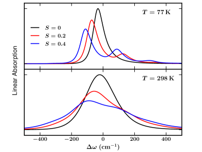
Figure 3: Linear absorption lineshapes of the excitonic monomer in Fig. 2 in the Condon limit at $77$ and $298$ K, for various Huang-Rhys factors.

Last but not least, we note that the appearance of the vibrational peaks may be caused by not only the non-Condon transition, but also the strong Franck–Condon vibronic coupling. In the latter case, the peaks are red shifted instead, as shown in Fig. 3. To distinguish the above two causes experimentally, one can examine the mirror symmetry between the absorption and emission spectroscopies.Orl734513 While the Franck–Condon approximation results in symmetric lineshapes, the non-Condon effects preferentially enhance the vibrational peaks on the blue side in both the absorption and emission spectroscopy.

III Results and Discussion

In this section, we discuss the simulation results of field-triggered EET dynamics and 2D spectroscopy for an excitonic dimer system. The system and bath parameters are as follows. The site energies are $\epsilon_{1}=12500$ ${\rm cm}^{-1}$ and $\epsilon_{2}=12300$ ${\rm cm}^{-1}$, and the dipole-dipole coupling is $V_{12}=-100$ ${\rm cm}^{-1}$. Each site is longitudinally subject to a diffusive solvent bath and a vibrational mode, which are characterized by a Drude model ($\lambda_{\mbox{\tiny D}}=40$ ${\rm cm}^{-1}$ and $\gamma_{\mbox{\tiny D}}=100$ ${\rm cm}^{-1}$), and an underdamped BO ($S=0.1$, $\omega_{\mbox{\tiny BO}}=200$ ${\rm cm}^{-1}$ and $\zeta_{\mbox{\tiny BO}}=10$ ${\rm cm}^{-1}$), respectively. Without loss of generality, we assume the two sites have the same dipole strength and set $\mu_{1}=\mu_{2}=\mu_{r}$ for the Condon part, and $\mu_{1}^{\prime}/\mu_{r}=\mu_{2}^{\prime}/\mu_{r}=0.1$ for the non-Condon part [cf. Eq. (17)], with $\mu_{r}$ being the reference dipole strength.

III.1 Field-triggered excitation energy transfer dynamics

Figure 4: Field-triggered EET dynamics for an excitonic dimer system at $77$ and $298$ K: Drude dissipation without vibronic coupling (black), with Franck–Condon coupling (red), and with Herzberg–Teller coupling (blue). The pulse is characterized by a Gaussian envelope $\mu_{r}\varepsilon(t)=\frac{\theta}{\sqrt{2\pi}\sigma}\exp(-\frac{t^{2}}{2\sigma^{2}})\cos(\omega_{c}t)$, with reference dipole strength $\mu_{r}$, flipping angle $\theta=0.05\pi$, temporal variance $\sigma=6$ fs, and carrier frequency $\omega_{c}=12400\,{\rm cm}^{-1}$.

In Fig. 4, we report the field-triggered population dynamics at three different conditions, including Drude dissipation without vibronic coupling, with Franck–Condon coupling, and with Herzberg–Teller coupling. It is observed that the time duration of the population oscillation is largely elongated by both Condon and non-Condon vibronic couplings. While the electronic decoherence with pure Drude dissipation lasts for about hundreds of  fs, the vibronic decoherence reaches above $1$ ps. The oscillation is weakened but still noticeable as the temperature increases.

We also find that the non-Condon vibronic coupling enhances the quantum yield of the excitonic system. This effect becomes more obvious at the room temperature ($298$  K), which indicates a stronger electronic-vibrational energy transfer therein. In comparison, the Condon vibronic coupling does not vary the final population significantly. This finding highlights the dynamical interplay between excitation of the system and non-Condon polarization of the vibrational environment.

In the meanwhile, it is shown that these two kinds of vibronic couplings result in similar population oscillation, indicating that the non-Condon vibronic coupling retains the electronic coherence of the reduced system. On the other hand, the total quantum coherence, including contributions from both reduced system and polarized vibrational environment, is enhanced, as discussed in the following section of the 2D spectroscopy simulations.

III.2 Coherent two dimensional spectroscopy

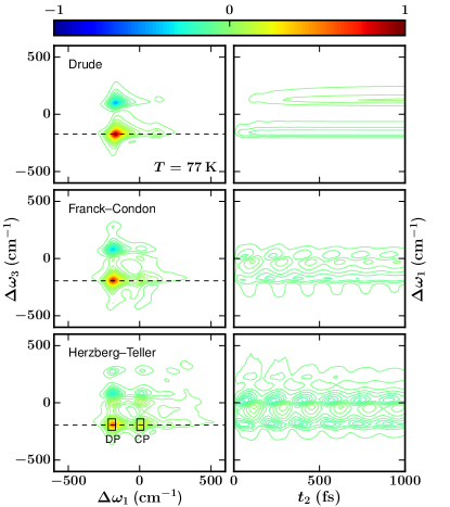
Figure 5: Two dimensional spectroscopy of the dimer system for Drude dissipation without vibronic coupling (top), with Franck–Condon coupling (middle) and with Herzberg-Teller coupling (bottom), at $77$ K. The left panels show the 2D signals at $t_{2}=0$, while the right panels show the $t_{2}$ dynamics of the signals along the dashed horizontal line. We set $\Delta\omega_{k}=\omega_{k}-(\epsilon_{1}+\epsilon_{2})/2$ for $k=1$ and $3$. All the results are scaled by the maximum of the pure Drude results, and in the right panels, the initial values at $t_{2}=0$ have been subtracted.

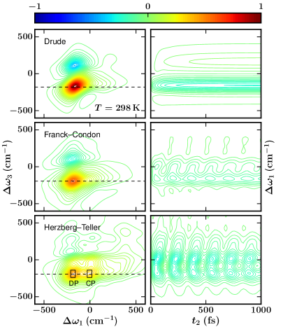
Figure 6: Two dimensional spectroscopy of the excitonic dimer in Fig. 5 at $298$ K. All the results are scaled by the maximum of the pure Drude results.

To investigate the dynamical electronic-vibrational interaction and the involving Condon and non-Condon effects, we further simulate the 2D spectroscopy for the dimer system. 2D coherent spectroscopy is a four-wave-mixing technique.Muk95 ; Muk042073 ; Muk091207 The multi-chromophore system is excited by three time-ordered laser pulses (with wavevectors ${\bf k}_{1}$ , ${\bf k}_{2}$ and ${\bf k}_{3}$) separated by time interval $t_{1}$ and $t_{2}$, and after a time-delay $t_{3}$, the emitted signal is measured along the phase matching direction ${\bf k}_{s}=\pm{\bf k}_{3}\pm{\bf k}_{2}\pm{\bf k}_{1}$. In this work, we simulate the pump-probe signal that consists of rephasing ${\bf k}_{\rm I}={\bf k}_{3}+{\bf k}_{2}-{\bf k}_{1}$ and non-rephasing ${\bf k}_{\rm II}={\bf k}_{3}-{\bf k}_{2}+{\bf k}_{1}$ configurations.Muk95 ; Muk042073 ; Muk091207 For simplicity, we adopt the rotating wave approximation and the impulsive limit. Muk95 ; Muk042073 ; Muk091207

The rephasing $S_{{\bf k}_{\rm I}}$ and non-rephasing $S_{{\bf k}_{\rm II}}$ signals are given by Muk95 ; Xu11497

$$S_{{\bf k}_{\rm I/II}}(\omega_{3},t_{2},\omega_{1}) ={\rm Re}\int_{0}^{\infty}\!\!\text{d}t_{3}\!\!\int_{0}^{\infty}\!\!\text{d}t_{1}e^{i(\omega_{3}t_{3}\mp\omega_{1}t_{1})}$$

$$\qquad\ \ \times R_{{\bf k}_{\rm I/II}}(t_{3},t_{2},t_{1}).$$ (20)

and related respectively to the nonlinear optical correlation functions

$$\begin{split}&R_{{\bf k}_{\rm I}}=R_{2}+R_{3}+R_{5}\qquad\text{\ \ \ (rephasing)}\,,\\ &R_{{\bf k}_{\rm II}}=R_{1}+R_{4}+R_{6}\qquad\text{(non-rephasing)}\,.\end{split}$$ (21)

In Eq. (21), the six Liouville-space pathways are expressed asXu11497 ; Zha16CP

$$\begin{split}R_{1}&=\langle\!\langle\hat{V}_{ge}(t_{3})|\overset{\leftarrow}{V}_{\!eg}{\cal G}_{ee}(t_{2})\overset{\leftarrow}{V}_{\!ge}{\cal G}_{eg}(t_{1})\overset{\rightarrow}{V}_{\!eg}|{\rho}^{\rm eq}_{\mbox{\tiny T},gg}\rangle\!\rangle,\\ R_{2}&=\langle\!\langle\hat{V}_{ge}(t_{3})|\overset{\leftarrow}{V}_{\!eg}{\cal G}_{ee}(t_{2})\overset{\rightarrow}{V}_{\!eg}{\cal G}_{ge}(t_{1})\overset{\leftarrow}{V}_{\!ge}|{\rho}^{\rm eq}_{\mbox{\tiny T},gg}\rangle\!\rangle,\\ R_{3}&=\langle\!\langle\hat{V}_{ge}(t_{3})|\overset{\rightarrow}{V}_{\!eg}{\cal G}_{gg}(t_{2})\overset{\leftarrow}{V}_{\!eg}{\cal G}_{ge}(t_{1})\overset{\leftarrow}{V}_{\!ge}|{\rho}^{\rm eq}_{\mbox{\tiny T},gg}\rangle\!\rangle,\\ R_{4}&=\langle\!\langle\hat{V}_{ge}(t_{3})|\overset{\rightarrow}{V}_{\!eg}{\cal G}_{gg}(t_{2})\overset{\rightarrow}{V}_{\!ge}{\cal G}_{eg}(t_{1})\overset{\rightarrow}{V}_{\!eg}|{\rho}^{\rm eq}_{\mbox{\tiny T},gg}\rangle\!\rangle,\\ R_{5}&=-\langle\!\langle\hat{V}_{ef}(t_{3})|\overset{\rightarrow}{V}_{\!fe}{\cal G}_{ee}(t_{2})\overset{\rightarrow}{V}_{\!eg}{\cal G}_{ge}(t_{1})\overset{\leftarrow}{V}_{\!ge}|{\rho}^{\rm eq}_{\mbox{\tiny T},gg}\rangle\!\rangle,\\ R_{6}&=-\langle\!\langle\hat{V}_{ef}(t_{3})|\overset{\rightarrow}{V}_{\!fe}{\cal G}_{ee}(t_{2})\overset{\leftarrow}{V}_{\!ge}{\cal G}_{eg}(t_{1})\overset{\rightarrow}{V}_{\!eg}|{\rho}^{\rm eq}_{\mbox{\tiny T},gg}\rangle\!\rangle.\end{split}$$ (22)

Here, all the involving operators and the propagator ${\cal G}(t)\equiv e^{-i{\cal L}_{\mbox{\tiny T}}t}$ are in their block forms subscripted by “$uv$”, where $u,v\in\{g,e,f\}$, with $|g\rangle$, $|e\rangle$ and $|f\rangle$ specifying the ground, singly-excited and doubly-excited electronic manifolds.Xu11497 The efficient evaluation of the DEOM-space equivalence of Eq. (22) follows Ref. Zha16CP, and Xu11497, . In our simulations, all parameters remain the same as those in Fig. 4.

Figure 5 demonstrates the simulated pump-probe spectroscopy at $77$ K under three circumstances, i.e. the pure Drude dissipation without vibronic coupling, the one with Franck–Condon coupling, and the one with Herzberg–Teller coupling. In the presence of the vibronic coupling, vibrational peaks on both diagonal and off-diagonal are observed, while the exciton-exciton off-diagonal peak is concealed. In particular, an electronic-vibrational cross peak (CP) appears right to the excitonic diagonal peak (DP) with the frequency difference around $\omega_{\mbox{\tiny BO}}$, as observed in the middle- and bottom-left panels of Fig. 5. It suggests that this CP measures the cross correlation between the first and the zeroth vibrational levels within the excited electronic state. With the non-Condon vibronic coupling, the above vibrational signals are more prominent. The right panels show the $t_{2}$ time-evolution of the signals along the dashed horizontal line, covering both the excitonic DP and the electronic-vibrational CP. With the vibronic coupling, the duration of the quantum beats is elongated obviously. As shown in the middle- and bottom-right panels, the vibronic CPs oscillate for at least 1 ps with both Condon and non-Condon vibronic couplings. For DPs, however, the oscillation with non-Condon coupling is more persistent than that with Condon coupling. Moreover, the non-Condon coupling results in larger oscillation amplitude. Evidently, the vibronic coupling facilitates the quantum coherence in the EET dynamics. In particular, the non-Condon transition greatly enhances the excitation of higher vibrational levels in the excited state. The subsequent vibrational energy relaxation preserves the long-lived coherence and amplifies the oscillation amplitudes in 2D spectroscopy.

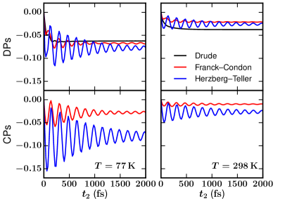
Figure 7: Amplitudes of the DPs and CPs along time interval $t_{2}$, extracted from the 2D spectroscopy with Franck–Condon coupling (black) and the Herzberg–Teller coupling (red) at $77$ and $298$ K. All curves are scaled by the maximum of pure Drude results at $77$ K and shifted vertically to make the initial values $0$.

In comparison with the results at $77$ K, the 2D signals at $298$ K are much broader, and the electronic and vibrational excitation peaks are not well separated, see Fig. 6. However, in the right panels, we observe similar dynamics of the excitonic DPs and electronic-vibrational CPs as those at $77$ K. Apparently, the vibrational energy relaxation at $298$ K is more prominent than that at $77$ K, see the middle-right and bottom-right panels in Fig. 5 and Fig. 6 for comparison.

In Fig. 7, we further compare the oscillation amplitudes at the cryogenic and room temperatures of the excitonic DPs and vibronic CPs along $t_{2}$, with all curves being scaled by the maximum of the pump-probe spectroscopy with pure Drude dissipation at cryogenic temperature ($77$ K). In both the Condon and non-Condon couplings, the quantum beats of the DPs and CPs last for more than $2$ ps , and their amplitudes are still noticeable at room temperauture ($298$ K), about one-third of those at $77$ K. In contrast, the quantum beats from purely electronic transitions are very short-lived, i.e., its coherence only lasts for 300 fs at $77$ K and becomes even more transient at $298$ K. Moreover, the non-Condon vibronic coupling further intensifies the vibrational oscillation amplitudes dramatically at both temperatures, in comparison with the Condon results.

Clearly, 2D spectroscopy detects both the excitonic system and the polarized vibrational environment. Our simulation results indicate that the vibronic coupling plays a dominant role in preserving the long-lived quantum beats, whereas the purely electronic coherence has minor contribution. This persistent quantum coherence is present at both cryogenic and room temperatures. Moreover, in comparison with the Condon counterpart, the non-Condon vibronic coupling greatly enhances the excitation of the higher vibrational levels in the excited electronic state, and the subsequent vibrational relaxation leads to the stronger quantum beats, in the $t_{2}$-resolved pump-probe spectroscopy.

IV Conclusion

In this work, we investigate the non-Condon virbonic coupling effects on the quantum coherence of the EET dynamics, via the non-perturbative DEOM simulations on excitonic model systems. Evidently, the DEOM is a unique theory in studying both the reduced system and the hybrid bath dynamics as well as their correlated quantum entanglement. Our simulations on field-triggered EET dynamics and coherent 2D spectroscopy show that the vibronic coupling elongates the quantum beats at both cryogenic and room temperatures. In particular, the non-Condon vibronic coupling facilitates the electronic-vibrational energy transfer and dramatically enhances the total system-and-bath quantum coherence. This work provides an insightful investigation on the origin of the quantum coherence, and may enrich the interpretation of the experimental nonlinear spectroscopy.

References

- (1) G. S. Engel et al., Nature 446, 782 (2007).
- (2) Y.-C. Cheng and G. R. Flemming, J. Phys. Chem. B 112, 4254 (2008).
- (3) G. Panitchayangkoon et al., Proc. Natl. Acad. Sci. USA 107, 12766 (2010).
- (4) M. B. Plenio, J. Almeida, and S. F. Huelga, J. Chem. Phys. 139, 235102 (2013).
- (5) D. B. Turner, K. E. Wilk, P. M. G. Curmi, and G. D. Scholes, J. Phys. Chem. Lett. 2, 1904 (2011).
- (6) R. Tempelaar, T. L. C. Jansen, and J. Knoester, J. Phys. Chem. B 118, 12865 (2014).
- (7) V. Butkus, L. Valkunas, and D. Abramavicius, J. Chem. Phys. 140, 034306 (2014).
- (8) F. V. A. Camargo, H. L. Anderson, S. R. Meech, and I. A. Heisler, J. Phys. Chem. A 119, 95 (2015).
- (9) V. Balevičius et al., Phys. Chem. Chem. Phys. 17, 19491 (2015).
- (10) T. Mančal et al., J. Phys. Chem. Lett. 3, 1497 (2012).
- (11) V. Perlík, C. Lincoln, F. Šanda, and J. Hauer, J. Phys. Chem. Lett. 5, 404 (2014).
- (12) Y. Fujihashi, G. R. Fleming, and A. Ishizaki, J. Chem. Phys. 142, 212403 (2015).
- (13) D. M. Monahan, L. Whaley-Mayda, A. Ishizaki, and G. R. Fleming, J. Chem. Phys. 143, 065101 (2015).
- (14) K. Ishii, S. Takeuchi, and T. Tahara, J. Phys. Chem. A 112, 2219 (2008).
- (15) P. Kambhampati, D. H. Son, T. W. Kee, and P. F. Barbara, J. Phys. Chem. A 104, 10637 (2000).
- (16) J. M. Womick, B. A. West, N. F. Scherer, and A. M. Moran, J. Phys. B: At. Mol. Opt. Phys. 45, 154016 (2012).
- (17) Y. Tanimura and R. Kubo, J. Phys. Soc. Jpn. 58, 101 (1989).
- (18) Y. A. Yan, F. Yang, Y. Liu, and J. S. Shao, Chem. Phys. Lett. 395, 216 (2004).
- (19) A. Ishizaki and Y. Tanimura, J. Phys. Soc. Jpn. 74, 3131 (2005).
- (20) Y. Tanimura, J. Phys. Soc. Jpn. 75, 082001 (2006).
- (21) Y. Tanimura, J. Chem. Phys. 141, 044114 (2014).
- (22) Y. Tanimura, J. Chem. Phys. 142, 144110 (2015).
- (23) R. X. Xu, P. Cui, X. Q. Li, Y. Mo, and Y. J. Yan, J. Chem. Phys. 122, 041103 (2005).
- (24) R. X. Xu and Y. J. Yan, Phys. Rev. E 75, 031107 (2007).
- (25) X. Zheng et al., Prog. Chem. 24, 1129 (2012), http://www.progchem.ac.cn/EN/abstract/abstract10858.shtml.
- (26) J. S. Jin, X. Zheng, and Y. J. Yan, J. Chem. Phys. 128, 234703 (2008).
- (27) L. P. Chen, R. H. Zheng, Y. Y. Jing, and Q. Shi, J. Chem. Phys. 134, 194508 (2011).
- (28) Y. J. Yan, J. Chem. Phys. 140, 054105 (2014).
- (29) H. D. Zhang, R. X. Xu, X. Zheng, and Y. J. Yan, J. Chem. Phys. 142, 024112 (2015).
- (30) J. S. Jin, S. K. Wang, X. Zheng, and Y. J. Yan, J. Chem. Phys. 142, 234108 (2015).
- (31) R. X. Xu, B. L. Tian, J. Xu, Q. Shi, and Y. J. Yan, J. Chem. Phys. 131, 214111 (2009).
- (32) K. B. Zhu, R. X. Xu, H. Y. Zhang, J. Hu, and Y. J. Yan, J. Phys. Chem. B 115, 5678 (2011).
- (33) J. J. Ding, J. Xu, J. Hu, R. X. Xu, and Y. J. Yan, J. Chem. Phys. 135, 164107 (2011).
- (34) J. J. Ding, R. X. Xu, and Y. J. Yan, J. Chem. Phys. 136, 224103 (2012).
- (35) H. D. Zhang and Y. J. Yan, J. Chem. Phys. 143, 214112 (2015).
- (36) R. X. Xu, H. D. Zhang, X. Zheng, and Y. J. Yan, Sci. China Chem. 58, 1816 (2015), Special Issue: Lemin Li Festschrift.
- (37) H. D. Zhang, Q. Qiao, R. X. Xu, and Y. J. Yan, Chem. Phys. (2016) doi: 10.1016/j.chemphys.2016.07.005.
- (38) G. Orlandi and W. Siebrand, J. Chem. Phys. 58, 4513 (1973).
- (39) S. H. Lin and H. Eyring, Proc. Nat. Acad. Sci. USA 71, 3802 (1974).
- (40) Y. Tanimura and S. Mukamel, J. Opt. Soc. Am. B 10, 2263 (1993).
- (41) Y. Tanimura and S. Mukamel, Phys. Rev. E 47, 118 (1993).
- (42) M. Thoss, H. B. Wang, and W. H. Miller, J. Chem. Phys. 115, 2991 (2001).
- (43) U. Weiss, Quantum Dissipative Systems, World Scientific, Singapore, 2008, 3rd ed. Series in Modern Condensed Matter Physics, Vol. 13.
- (44) Y. J. Yan and R. X. Xu, Annu. Rev. Phys. Chem. 56, 187 (2005).
- (45) S. Mukamel, The Principles of Nonlinear Optical Spectroscopy, Oxford University Press, New York, 1995.
- (46) R. P. Feynman and F. L. Vernon, Jr., Ann. Phys. 24, 118 (1963).
- (47) J. Xu, R. X. Xu, D. Abramavicius, H. D. Zhang, and Y. J. Yan, Chin. J. Chem. Phys. 24, 497 (2011).
- (48) J. Xu, H. D. Zhang, R. X. Xu, and Y. J. Yan, J. Chem. Phys. 138, 024106 (2013).
- (49) S. Mukamel and D. Abramavicius, Chem. Rev. 104, 2073 (2004).
- (50) S. Mukamel, Y. Tanimura, and P. Hamm, Special Issue of Acc. Chem. Res. 42, 1207 (2009).