Temperature fluctuations in canonical systems: Insights from molecular dynamics simulations

Abstract

Molecular dynamics simulations of a quasi-harmonic solid are conducted to elucidate the meaning of temperature fluctuations in canonical systems and validate a well-known but frequently contested equation predicting the mean square of such fluctuations. The simulations implement two virtual and one physical (natural) thermostat and examine the kinetic, potential and total energy correlation functions in the time and frequency domains. The results clearly demonstrate the existence of quasi-equilibrium states in which the system can be characterized by a well-defined temperature that follows the mentioned fluctuation equation. The emergence of such states is due to the wide separation of timescales between thermal relaxation by phonon scattering and slow energy exchanges with the thermostat. The quasi-equilibrium states exist between these two timescales when the system behaves as virtually isolated and equilibrium.

I Introduction

Fluctuations of thermodynamic properties play an important role in phase transformations and many other physical phenomena and diverse applications. While fluctuations of energy $E$, volume $V$, number of particles $N$ and other extensive parameters are well-understood, controversies remain regarding the nature, or even existence,(Kittel and Kroemer, 2000; Kittel, 1973, 1988) of fluctuations of intensive parameters such as temperature, pressure and chemical potentials. In particular, the question of temperature fluctuations in canonical systems has been the subject of discussions for over a century (see e.g. van Hemmen and Longtin(van Hemmen and Longtin, 2013) for a historical overview of the subject).

A number of different views on temperature fluctuations can be found in the literature, including the following:

(i) Temperature fluctuations in canonical systems is a real physical phenomenon and can be measured experimentally.(Chiu et al., 1992) If the volume and number of particles in the system are fixed, then(Landau and Lifshitz, 2000; Callen, 1985; Mishin, 2015)

$$\left\langle(\Delta T)^{2}\right\rangle=\dfrac{kT_{0}^{2}}{Nc_{v}^{0}},$$ (1)

where $\Delta T=T-T_{0}$ is the deviation of the system temperature $T$ from the thermostat temperature $T_{0}$, $c_{v}^{0}$ is the constant-volume specific heat (per particle) at the temperature $T_{0}$, and $k$ is Boltzmann’s constant. The angular brackets $\left\langle...\right\rangle$ indicate the canonical ensemble average. Assuming ergodicity, $\left\langle...\right\rangle$ can be computed by averaging over a long trajectory in the phase space of the system. Spontaneous energy exchanges between the system and the thermostat bring the system to quasi-equilibrium states in which the temperature is slightly higher or slightly lower than $T_{0}$. It is also possible to quantify the cross-correlation between the fluctuating temperature and the system’s total energy by the equation(Landau and Lifshitz, 2000; Callen, 1985; Mishin, 2015)

$$\left\langle\Delta E\Delta T\right\rangle=kT_{0}^{2},$$ (2)

where $\Delta E=E-E_{0}$ and $E_{0}$ is the equilibrium energy.

(ii) Temperature of a canonical system is defined as the temperature of the thermostat. Thus, $T\equiv T_{0}$ by definition and the very notion of temperature fluctuations is meaningless.(Kittel, 1973, 1988; Kittel and Kroemer, 2000)

(iii) While fluctuations of the system energy $E$ are well-defined, non-equilibrium temperature $T$ is ill-defined.(van Hemmen and Longtin, 2013; Kittel, 1988) One can formally define $T$ as $T\equiv T_{0}+(E-E_{0})/(Nc_{v}^{0})$, which makes $T$ just a nominal parameter identical to energy.(van Hemmen and Longtin, 2013) From this point of view, equation (1) contains no new physics in comparison with the well-established energy fluctuation relation(Landau and Lifshitz, 2000; Callen, 1985; Mishin, 2015)

$$\left\langle(\Delta E)^{2}\right\rangle=NkT_{0}^{2}c_{v}^{0}.$$ (3)

(iv) Even for an equilibrium isolated system, temperature is not a well-defined parameter. It can be evaluated by measuring the system energy and trying to estimate the temperature of the thermostat with which the system was in equilibrium before being disconnected.(Mandelbrot, 1989; Falcioni et al., 2011) This reduces the temperature definition to a statistical problem addressed in the framework of the estimation theory. The statistical uncertainty associated with the temperature estimate can be interpreted as its “fluctuation”.

Recently, thermodynamics-based arguments for the viewpoint (i) have been put forward as part of a more general thermodynamic fluctuation theory.(Mishin, 2015) The goal of the present paper is to provide additional insights into the nature of temperature fluctuations by conducting molecular dynamics (MD) simulations of a quasi-harmonic crystalline solid. As an operational definition, the non-equilibrium temperature is identified with kinetic energy of the particles averaged on an appropriate timescale. In Sec. II we set the stage by reviewing the thermodynamic arguments(Landau and Lifshitz, 2000; Callen, 1985; Mishin, 2015) and introducing three timescales of the problem that permit a clear definition of non-equilibrium temperature. After presenting the simulation methodology in Sec. III, we report on MD results for the kinetic, potential and total energy fluctuations and the respective correlation functions for the solid (Sec. IV). Using this data, we are able to extract the temperature fluctuations and verify Eqs.(1) and (2) independently of Eq.(3). In Sec. V we summarize the results of this work and formulate conclusions.

II Theory

If a thermodynamic system is disconnected from its environment and becomes isolated, it reaches thermodynamic equilibrium after a characteristic relaxation time $\tau_{r}$. For a simple system, the equilibrium state is fully defined by its energy $E$, volume $V$ and number of particles $N$. The entropy $S$ of an equilibrium isolated system is a function of $E$, $V$, and $N$. This function can be established by equilibrating the isolated system with different values of $E$, $V$ and $N$ and measuring or computing $S$ for each set of these parameters. The function $S=S(E,V,N)$ is called the fundamental equation(Gibbs, 1948; Callen, 1985; Mishin, 2015) and incapsulates all thermodynamic properties of the substance. The temperature, pressure and chemical potential are defined by the fundamental equation as the derivatives $T=1/(\partial S/\partial E)$, $p=T(\partial S/\partial V)$ and $\mu=-T(\partial S/\partial N)$, respectively.

Suppose the isolated system is still in the process of relaxation. While $E$, $V$ and $N$ are fixed, other thermodynamic properties can vary. If we mentally partition the system into relatively small subsystems, their parameters $E$, $V$ and $N$ can vary during the relaxation. It is important to recognize that the relaxation time $t_{r}$ of a small subsystem is much shorter than $\tau_{r}$ of the entire system, at least for short-range interatomic forces. Thus, there is a certain timescale $t_{q}$ such that

$$t_{r}\ll t_{q}\ll\tau_{r},$$ (4)

on which the small subsystems remain infinitely close to equilibrium, even though the entire system is not in full equilibrium. The subsystems weakly interact with each other across their interfaces, causing a slow drift of the entire system towards equilibrium. Such virtually equilibrium subsystems are called quasi-equilibrium(Mishin, 2015) and the entire isolated system is said to be in a quasi-equilibrium state. On the quasi-equilibrium timescale $t_{q}$, the isolated system can be thought of as equilibrated in the presence of isolating walls separating its small subsystems. Accordingly, each quasi-equilibrium subsystem $\alpha$ can be described by a fundamental equation $S_{\alpha}=S_{\alpha}(E_{\alpha},V_{\alpha},N_{\alpha})$, from which the local temperature, pressure and chemical potential can be found by $T_{\alpha}=1/(\partial S_{\alpha}/\partial E_{\alpha})$, $p_{\alpha}=T_{\alpha}(\partial S_{\alpha}/\partial V_{\alpha})$ and $\mu_{\alpha}=-T_{\alpha}(\partial S_{\alpha}/\partial N_{\alpha})$, respectively. If the number of subsystems is large enough, we can talk about spatially continuous temperature, pressure and chemical potential fields. Such fields appear in the standard treatments of irreversible thermodynamics(De Groot and Mazur, 1984) and are only defined on the quasi-equilibrium timescale. They evolve during the relaxation process and eventually become uniform when the entire system reaches equilibrium.

Following the fluctuation-dissipation concepts,(Landau and Lifshitz, 2000; Nyquist, 1928; Onsager, 1931a, b; Callen and Welton, 1951; Kubo, 1966; Marconi et al., 2008) one can expect that similar quasi-equilibrium states arise during equilibrium fluctuations in an isolated system. Accordingly, the fluctuated states can be described by well-defined local values of the intensive parameters, including temperature. Again, such local intensive parameters are only defined on the quasi-equilibrium timescale $t_{q}$.

Turning to canonical fluctuations, consider a small subsystem of an equilibrium isolated system. Let us call this subsystem a system and the rest of the isolated system a reservoir. Consider a timescale $t_{q}$ such that $t_{r}\ll t_{q}\ll\tau_{r}$, where $t_{r}$ is the relaxation time of the system and $\tau_{r}$ is the global relaxation time of the system plus reservoir. On this timescale, the system can be considered as quasi-equilibrium and thus virtually isolated. As such, it possess all intensive properties mentioned above. Fluctuations generally occur on all timescales. However, if we monitor the system properties averaged over the timescale $t_{q}$, then we can talk about fluctuations of its intensive parameters. In particular, quasi-equilibrium fluctuations that preserve the system volume and number of particles (canonical ensemble) include well-defined temperature fluctuations. As long as the temperature is properly defined on the quasi-equilibrium timescale, it will satisfy the fluctuation relation (1).

We next apply these concepts to a crystalline solid comprising a fixed number of atoms $N\gg 1$. The local relaxation timescale $t_{r}$ can be identified with a typical phonon lifetime. Suppose the solid is isolated and in equilibrium. Its instantaneous potential energy $U$ and kinetic energy of the centers of mass of the particles $K$ fluctuate whereas the total energy $E=K+U$ is strictly fixed. The timescale $t_{K}$ of the kinetic (as well as potential) energy fluctuations is the inverse of a typical phonon frequency $\bar{f}$: $t_{K}\sim 1/\bar{f}$. Assuming that the solid is nearly harmonic, this timescale is much shorter than $t_{r}$. The temperature of the solid is fixed at $T=E/3k$ and can be evaluated from the equipartition relation $\left\langle K\right\rangle=3NkT/2$ by monitoring the kinetic energy over a long time $t\gg t_{r}$.

If the same solid is now connected to a thermostat, two types of fluctuation occur. First, the same fluctuations as in the isolated system, including the energy exchanges between the phonon modes on the $t_{r}$ timescale. Second, there will be fluctuations in the total energy of the solid due to energy exchanges between the solid and the thermostat. The two types of fluctuation are governed by physically different relaxation processes: phonon scattering inside the solid in the first case and heat flow between the solid and the thermostat in the second. The respective relaxation times, $t_{r}$ and $\tau_{r}$, are significantly different. Usually $\tau_{r}\gg t_{r}$, i.e., the energy exchanges with the thermostat occur on a much longer timescale that depends on the system size, the system/thermostat interface and other factors. Thus, there is a timescale $t_{q}$ in between, $t_{r}\ll t_{q}\ll\tau_{r}$, on which the solid remains quasi-equilibrium and can be assigned a well-defined temperature. We can use the equipartition relation to find this quasi-equilibrium temperature,

$$T=\dfrac{2\left\langle K\right\rangle_{q}}{3Nk},$$ (5)

where the subscript $q$ indicates that the time average must be taken on the quasi-equilibrium timescale $t_{q}$.

If the kinetic energy is averaged over the thermodynamic timescale $t\gg\tau_{r}$, then the equipartition relation trivially gives the thermostat temperature

$$T_{0}=\dfrac{2\left\langle K\right\rangle}{3Nk}.$$ (6)

By contrast, the quasi-equilibrium temperature defined by Eq.(5) fluctuates around $T_{0}$ and is predicted to satisfy the fluctuation formula (1). We emphasize that Eq.(5) defines $T$ independently of the instantaneous or average values of the total energy and makes no reference to the specific heat of the substance. Instead, the temperature fluctuations can be used to extract the specific heat $c_{v}^{0}$. For a classical harmonic solid composed of atoms (not a molecular crystal), $c_{v}^{0}=3k$ and Eq.(1) becomes

$$\left\langle(\Delta T)^{2}\right\rangle=\dfrac{T_{0}^{2}}{3N}.$$ (7)

The key point of this treatment is that the kinetic energy of the centers of mass of the particles must be averaged over the appropriate timescale. We caution against using the “instantaneous temperature” defined by the instantaneous value of the kinetic energy as $\hat{T}=2K/3Nk$, as is often done in the MD community. The “temperature” $\hat{T}$ so defined essentially represents the kinetic energy $K/N$ itself up to units. Although this unit conversion can sometimes make the MD results look more intuitive, it fails to predict the correct temperature fluctuations. Using the standard canonical distribution, it is easy to show that for any classical system(Lebowitz et al., 1967)

$$\left\langle(\Delta K)^{2}\right\rangle=\dfrac{3N(kT_{0})^{2}}{2},$$ (8)

from which

$$\left\langle(\Delta\hat{T})^{2}\right\rangle=2\dfrac{T_{0}^{2}}{3N}.$$ (9)

For an atomic solid, this equation is off by a factor of two. Consequently, the specific heat of the solid extracted from Eq.(1) using the “instantaneous temperature” $\hat{T}$ is $3k/2$ instead of the correct $3k$.

In spite of the failure of the “instantaneous temperature” $\hat{T}$ to describe the mean-square fluctuation of temperature, it does satisfy some other fluctuation relations, including Eq.(2) which then becomes $\left\langle\Delta E\Delta\hat{T}\right\rangle=kT_{0}^{2}$. Like the energy variance $\left\langle(\Delta E)^{2}\right\rangle$, the covariance $\left\langle\Delta E\Delta T\right\rangle$ remains the same for both instantaneous and quasi-equilibrium fluctuations.

In the following sections, Eqs.(1), (2) and (3) will be verified by MD simulations with different choices of the thermostat.

III Methodology of simulations

III.1 Molecular dynamics simulations

As a model system we chose face-centered cubic copper with atomic interactions described by an embedded-atom potential.(Mishin et al., 2001) The potential accurately reproduces many physical properties of Cu, including phonon dispersion relations. The MD simulations were performed with the LAMMPS code(Plimpton, 1995) with the time integration step of $dt=0.001$ ps. Except for the system in a “natural thermostat” discussed later, all simulations were conducted in a cubic simulation block with periodic boundary conditions. The block edge was 7.23 nm and the total number of atoms was $N=32000$. The block edges were aligned with $\left\langle 100\right\rangle$ directions of the crystal lattice. The simulation temperature was chosen to be $T_{0}=100$ K and the lattice parameter was adjusted to ensure that the solid was stress-free at this temperature.

Prior to studying thermal fluctuations, two types of additional simulations were performed to generate data needed for a comparison with fluctuation results. Firstly, the phonon density of states $g(f)$ at 100 K was computed by the method developed by Kong(Kong, 2011) and implemented in LAMMPS. This method was chosen because it does not rely on fluctuations and provides independent results for comparison. Secondly, to test the accuracy of the simulation methodology, the specific heat of the solid was computed by a direct (non-fluctuation) method. This was accomplished by running canonical (NVT) MD simulations at the temperatures of 50, 100 and 150 K and calculating the time average energies $\left\langle E\right\rangle$. The volume was fixed at the value corresponding to 100 K. The energy was found to follow a linear temperature dependence in this temperature interval, from which the derivative $(\partial\left\langle E\right\rangle/\partial T)_{N,V}$ was evaluated by a linear fit. The specific heat at 100 K was then found from the equation $c_{v}^{0}=(\partial\left\langle E\right\rangle/\partial T)_{N,V}/N$. The number obtained was $24.89$ J/(mol K), which is close to the equipartition theorem prediction $3k=24.94$ J/(mol K).

The subsequent MD simulations utilized two ensembles: the microcanonical NVE (isolated system) and canonical NVT (system in a thermostat). The NVE system was prepared so that the temperature evaluated from the relation $\left\langle K\right\rangle_{NVE}=3NkT/2$ was very close to 100 K. In the NVE ensemble, the MD simulation simply integrates the classical equations of motion with a Hamiltonian dictated by the interatomic potential. The NVT simulations utilized the Langevin thermostat built into LAMMPS.(Plimpton, 1995) The Langevin algorithm(Frenkel and Smit, 2002) mimics a thermostat by treating the atoms as if they were embedded in an artificial viscous medium composed of much smaller particles. This medium exerts a drag force as well as a stochastic noise force $\boldsymbol{R}$ that constantly perturbs the atoms. The total force on atom $i$ is

$$\boldsymbol{F}_{i}=-\frac{\partial U(\boldsymbol{r}_{1}...\boldsymbol{r}_{N})}{\partial\boldsymbol{r}_{i}}-m_{i}\gamma\boldsymbol{v}_{i}+\boldsymbol{R}_{i}.$$ (10)

Here, $U(\boldsymbol{r}_{1}...\boldsymbol{r}_{N})$ is the potential energy due to atomic interactions, and $m_{i}$, $\boldsymbol{r}_{i}$ and $\boldsymbol{v}_{i}$ are, respectively, the mass, position and velocity of atoms $i$. The drag term depends on the damping constant $\gamma$, the inverse of which controls the timescale $\tau_{r}$ of the energy exchanges between the solid and the thermostat. During the simulation, the noise $\boldsymbol{R}_{i}$ is randomly sampled from a normal or uniform distribution at time intervals much shorter than $\tau_{r}=1/\gamma$. The variance of the noise defines the thermostat temperature $T_{0}$ via the standard fluctuation-dissipation relation.(Frenkel and Smit, 2002) To evaluate the role of the thermostat, additional simulations were conducted with a Nose-Hoover thermostat as will be discussed later.

III.2 Post-processing procedures

We next describe the statistical analysis of the MD results at the post-processing stage. Consider a long MD simulation run implemented for a time $t_{\mathrm{tot}}$. Suppose two fluctuating properties, $X$ and $Y$, are saved at every integration step of the simulation. These can be the kinetic, potential or total energy of the solid. We trivially compute the time average values $\left\langle X\right\rangle$ and $\left\langle Y\right\rangle$, as well as the variances $\langle(\Delta X)^{2}\rangle$ and $\langle(\Delta Y)^{2}\rangle$ and the covariance $\langle\Delta X\Delta Y\rangle$, were $\Delta X=X-\left\langle X\right\rangle$ and $\Delta Y=Y-\left\langle Y\right\rangle$.

For a spectral analysis, we break the long stochastic processes $X(t)$ and $Y(t)$ into a large number of shorter processes, $x(t)$ and $y(t)$, by dividing the total time $t_{\mathrm{tot}}$ into smaller intervals of the same duration $\theta\ll t_{\mathrm{tot}}$. The time $\theta$ was chosen to be longer than the correlation times of both variables, so that the intervals represent statistically independent samples with different initial conditions. For each time interval $0\leq t\leq\theta$ we perform a discrete Fourier transformation of $x(t)$ and $y(t)$ to obtain a set of Fourier amplitudes, $\hat{x}_{j}$ and $\hat{y}_{j}$, corresponding to the frequencies $f_{j}=j/\theta$, where $j=0,\pm 1,\pm 2,...$. These amplitudes are complex numbers satisfying the symmetry relations $\hat{x}_{-j}=\hat{x}_{j}^{*}$ and $\hat{y}_{-j}=\hat{y}_{j}^{*}$ (the asterisk denotes complex conjugation). The functions

$$\hat{C}_{XX}(f_{j})=\frac{\overline{\hat{x}_{j}\hat{x}_{j}^{*}}}{f_{1}},\qquad\hat{C}_{YY}(f_{j})=\frac{\overline{\hat{y}_{j}\hat{y}_{j}^{*}}}{f_{1}},$$

where the bar denotes averaging over all time intervals, represent the ensemble-averaged power spectra of $X$ and $Y$. Likewise,

$$\hat{C}_{XY}(f_{j})=\frac{\overline{\hat{x}_{j}\hat{y}_{j}^{*}}}{f_{1}}$$

represents the spectral power of $X$-$Y$ correlations.

Following the Wiener-Khinchin theorem,(Landau and Lifshitz, 2000; Kubo et al., 1991) the functions $\hat{C}_{XX}(f_{j})$, $\hat{C}_{YY}(f_{j})$ and $\hat{C}_{XY}(f_{j})$ were then subject to inverse Fourier transformations to obtain the auto-correlation functions (ACF) $C_{XX}(t)=\left\langle X(0)X(t)\right\rangle$ and $C_{YY}(t)=\left\langle Y(0)Y(t)\right\rangle$ and the cross-correlation function (CCF) $C_{XY}(t)=\left\langle X(0)Y(t)\right\rangle$. In this work, we are interested in correlations between properties relative to their average values, namely, $C_{\Delta X\Delta X}(t)=\left\langle\Delta X(0)\Delta X(t)\right\rangle$, $C_{\Delta Y\Delta Y}(t)=\left\langle\Delta Y(0)\Delta Y(t)\right\rangle$ and $C_{\Delta X\Delta Y}(t)=\left\langle\Delta X(0)\Delta Y(t)\right\rangle$. These were readily obtained by removing the point $f_{0}$ from the spectra prior to the Fourier inversion.

All correlation functions in the frequency domain shown in the figures below have been normalized by $\langle(\Delta X)^{2}(\Delta Y)^{2}\rangle^{1/2}$. For ACFs, the area under the normalized plots agains the frequency is therefore unity.

To evaluate the effect of the averaging timescale on the fluctuation relations more directly, the spectral analysis was supplemented by a simple coarse-graining procedure in the time domain. For this procedure, we lifted the requirement that the time interval $\theta$ be longer than the correlation time. For every time interval $l$, we computed the time average energy values $\left\langle X\right\rangle_{l}$, $\left\langle Y\right\rangle_{l}$, etc. A formal temperature $T_{l}$ was defined by the equipartition relation $T_{l}=2\left\langle K\right\rangle_{l}/3Nk$. These coarse-grained values were then treated as a new dataset, for which we computed the fluctuation properties such as $\langle(\Delta E)^{2}\rangle_{\theta}$, $\langle(\Delta T)^{2}\rangle_{\theta}$ and $\langle\Delta E\Delta T\rangle_{\theta}$. These fluctuation properties were examined as functions of the time interval $\theta$. For $\theta=dt$, this procedure reduces to computing the fluctuations of instantaneous properties. By increasing $\theta$, we can scan various timescales, including $t_{r}$, $\tau_{r}$, and the quasi-equilibrium timescale in between.

IV Simulation results and discussion

IV.1 NVE simulations

The goal of the NVE simulations was to evaluate the phonon relaxation time at the chosen temperature and make consistency checks of the methodology. Figure 1 shows the kinetic energy ACF in the frequency and time domains. The results were obtained from a $t_{\mathrm{tot}}=2$ ns MD run by averaging over $\theta=3$ ps time intervals. For comparison, the plot of $\hat{C}_{\Delta K\Delta K}(f)$ [Fig. 1(a)] includes the phonon density of states $g(f/2)$ computed by the non-fluctuation method(Kong, 2011) and plotted against the frequency $f$ followed by normalization to unit area. The close similarity between the plots is not surprising: in a perfectly harmonic solid, the kinetic energy ACF is identical to the phonon density of states except for the doubling of the frequency scale.(Dicky and Paskin, 1969; Scheidler et al., 2001; Hickman and Mishin, 2016) This doubling is due to the fact that kinetic energy goes through zero twice per vibration period. In the present simulations, the vibrations were not perfectly harmonic. The anharmonicity slightly washed out the shape of the spectrum and produced a high-frequency tail. Since the total energy is strictly conserved, the potential energy ACF has an identical shape (not shown here). As another test, the velocity ACF $\hat{C}_{vv}(f)$ was computed from the same simulation run. As expected, it was found to be very similar to $\hat{C}_{\Delta K\Delta K}(f)$ except for the frequency doubling effect: $\hat{C}_{vv}(f/2)\approx g(f/2)\approx\hat{C}_{\Delta K\Delta K}(f)$.

(a)

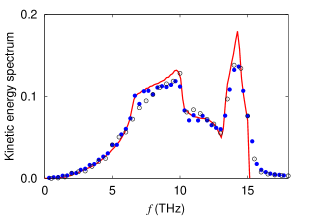
(b)

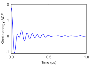
Figure 1: Results of NVE MD simulations. (a) Normalized power spectrum $\hat{C}_{\Delta K\Delta K}(f)$ of kinetic energy fluctuations (filled circles), velocity ACF $\hat{C}_{vv}(f/2)$ (open circles), and phonon density of states $g(f/2)$ (solid line). (b) The kinetic energy ACF $C_{\Delta K\Delta K}(t)$.

The time-dependent ACF $C_{\Delta K\Delta K}(t)$ shown in Fig. 1(b) indicates that the relaxation time due to phonon scattering is about 0.5 ps. Strictly speaking, this time depends on the phonon frequency and polarization, but we are only interested in a crude estimate. For comparison, the period $t_{K}$ of kinetic energy fluctuations can be estimated using a typical frequency of $\bar{f}=10$ THz [Fig. 1(a)], which gives about $t_{K}\approx 0.1$ ps. The factor of five difference between the two timescales is a measure of anharmonicity of this solid at 100 K.

In the NVE ensemble, the variance of the kinetic energy of the centers of mass of the particles is(Lebowitz et al., 1967)

$$\langle(\Delta K)^{2}\rangle_{NVE}=\frac{3N(kT_{0})^{2}}{2}\left(1-\frac{3k}{2c_{v}^{0}}\right).$$ (11)

Using $\langle(\Delta K)^{2}\rangle_{NVE}$ obtained by the simulation, this equation was inverted to solve for $c_{v}^{0}$. The number obtained was $25.06$ J/(mol K), which is in good agreement with $24.94$ J/(mol K) predicted by the equipartition theorem.

We emphasize that equilibrium temperature fluctuations in the NVE ensemble are undefined since quasi-equilibrium states are only sampled by small subsystems of the system but not the system as a whole. As already mentioned, one can always formally define an “instantaneous temperature” $\hat{T}$ and its fluctuations, but this temperature is identical (up to units) to the instantaneous kinetic energy per atom and does not provide new physical insights.

IV.2 NVT simulations

The NVT MD simulations were conducted with two time constants of the Langevin thermostat: $\tau_{r}=10$ and $100$ ps. The simulations times were $t_{\mathrm{tot}}=1000\tau_{r}$ (10 and 100 ns, respectively). The kinetic and total energy fluctuations are illustrated in Fig. 2. To facilitate the comparison, the energies were shifted relative to their time average values and normalized by standard deviations. The plots clearly demonstrate the existence of two different fluctuation processes: fast fluctuations of kinetic energy and much slower fluctuations of total energy. The fast fluctuations occur on the timescale of phonon frequencies, whereas the slow fluctuations occur on the thermostat timescale $\tau_{r}$. The large disparity between the two timescales is demonstrated in the insets, where the kinetic energy fluctuations are superimposed on nearly constant total energy. This two-scale behavior is especially manifest for the slower thermostat ($\tau_{r}=100$ ps) and is a clear signature of quasi-equilibrium states, in which the system behaves as if it were isolated and thus maintained a constant energy.

(a)

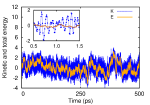
(b)

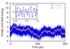
Figure 2: Representative fluctuations of the kinetic (blue) and total (orange) energy in the NVT ensemble with the thermostat time constants (a) $\tau_{r}=10$ ps and (b) $\tau_{r}=100$ ps. To enable comparison, the energies were shifted relative to the average values and normalized by the standard deviations. The insets zoom into shorter time intervals to demonstrate the existence of two different timescales of the fluctuations (fast and slow).

Figures 3(a,b) show the results of the timescale analysis discussed in Sec. III.2, in which the energies were averaged over different time intervals $\theta$ before computing their fluctuations (Fig. 3(c) will be discussed later). The variances/covariances $\langle(\Delta T)^{2}\rangle_{\theta}$, $\langle\Delta E\Delta T\rangle_{\theta}$ and $\langle(\Delta E)^{2}\rangle_{\theta}$ are compared with the right-hand sides of Eqs.(1), (2) and (3), respectively. The deviation is normalized by the value of the right-hand side and plotted against $\theta$. Recall that the minimum value of $\theta$ is the integration step $dt$, corresponding to instantaneous values of the energies. Observe that the “instantaneous temperature” fluctuation $\left\langle(\Delta\hat{T})^{2}\right\rangle$ has a 50% error. This number is consistent with the theoretical prediction in Sec. II that an estimate of temperature fluctuations from $\hat{T}$ will be off by a factor of two. As the averaging time $\theta$ increases, the error diminishes. When $\theta$ exceeds the phonon relaxation time $t_{r}$ (about 0.5 ps), the error reduces to $\pm$ a few percent and remains on this low level until $\theta$ approaches the thermostat time $\tau_{r}$. At that point the error increases again since the averaging begins to smooth the temperature fluctuations. In the limit of $\theta\rightarrow\infty$, all fluctuations are totally suppressed and the error goes to 100%. This behavior clearly demonstrates the existence of a timescale on which the temperature defined by the average kinetic energy satisfies the fluctuation relation (1). As predicted in Sec. II, this timescale lies between $t_{r}$ and $\tau_{r}$ where the system samples quasi-equilibrium states. Comparing Figs. 3(a) and 3(b), we observe that the range of validity of Eq.(1) widens as the thermostat time $\tau_{r}$ increases at a fixed $t_{r}$, which is again consistent with the definition of quasi-equilibrium states. By contrast, the errors in $\langle\Delta E\Delta T\rangle_{\theta}$ and $\langle(\Delta E)^{2}\rangle_{\theta}$ remain negligible on all timescales until $\theta$ approaches $\tau_{r}$ and the averaging begins to suppress the fluctuations. This is also fully consistent with the theory. As discussed in Sec. II, Eqs.(2) and (3) remain valid for both instantaneous and quasi-equilibrium values of the fluctuating properties, which is consistent with Figs. 3(a,b).

(a)

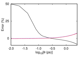
(b) 

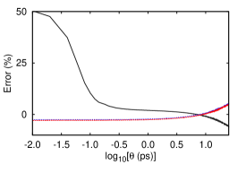
(c)

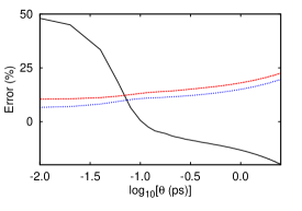
Figure 3: Normalized difference between the right and left-hand sides of fluctuation relations as functions of the averaging time interval $\theta$: Eq.(1) (black solid line), Eq.(2) (red dashed line) and Eq.(3) (blue dotted line) . (a) Langevin thermostat with $t_{r}=10$ ps, (b) Langevin thermostat with $t_{r}=100$ ps, (c) natural thermostat.

Turning to the spectral analysis of the fluctuations, Fig. 4 presents the power spectra of the kinetic and potential energies for the two Langevin thermostats. For the total energy, the spectrum shows a monotonic decay with frequency and dies off at frequencies larger than $1/\tau_{r}$, which supports the notion that the total energy fluctuations are primarily caused by slow exchanges with the thermostat. By contrast, the kinetic energy spectrum consists of two parts separated by a frequency gap. The low-frequency part is very similar to that for the total energy, suggesting a strong correlation. The high-frequency part has a shape of the phonon spectrum (plotted as a function of $2f$) and is virtually identical to the spectrum computed in the NVE ensemble (cf. Fig. 1). Note also that the high-frequency part of the spectrum is the same regardless of the thermostat time constant. This part of the spectrum is dominated by the phonon processes and is independent of how and whether the system interacts with environment. The gap between the low and high-frequency parts of the spectrum is where the system is found in quasi-equilibrium states. As expected, this gap widens as $\tau_{r}$ increases.

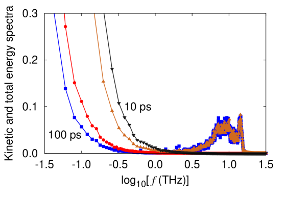
Figure 4: Normalized power spectra of kinetic and total energy fluctuations in the NVT ensemble with a Langevin thermostat for two different time constants (10 and 100 ps). Square and triangle symbols - kinetic energy, circle and nabla symbols - total energy.

The kinetic-potential and kinetic-total CCFs in the frequency domain are plotted in Fig. 5. The respective ACFs are also shown for comparison. Note that, at high frequencies, the kinetic-potential energy CCF $\hat{C}_{\Delta K\Delta U}(f)$ is a mirror image of the kinetic energy ACF $\hat{C}_{\Delta K\Delta K}(f)$ [Fig. 5(a)]. This reflects the nearly perfect anti-correlation between the two energies on the phonon timescale where the energy exchanges with the thermostat are negligible and the solid behaves as if it were isolated. In the low-frequency range below the gap, $\hat{C}_{\Delta K\Delta U}(f)$ and $\hat{C}_{\Delta K\Delta K}(f)$ practically coincide. This is also expected since the energy exchanges with the thermostat increase or decrees the kinetic and potential energies (averaged over the phonon timescale) simultaneously. Although these correlation functions are only shown for $\tau_{r}=10$ ps, the results for $\tau_{r}=100$ ps look very similar except for a wider frequency gap. On the other hand, the $\hat{C}_{\Delta K\Delta E}(f)$ and $\hat{C}_{\Delta E\Delta E}(f)$ correlation functions are similar for all frequencies [Fig. 5(b)]. In the low-frequency range, this is consistent with the correlated behavior of all components of energy during the thermostat exchanges. At high frequencies, the fast fluctuations of kinetic energy and nearly constant total energy produce a zero CCF. Since both correlation functions are strongly dominated by low frequencies, $\langle(\Delta E)^{2}\rangle$, $\langle\Delta E\Delta K\rangle$ and $\langle\Delta E\Delta T\rangle$ remain the same on both the instantaneous and quasi-equilibrium timescales.

Figure 6 shows the correlation functions in the time domain. Again, only the functions for $\tau_{r}=10$ ps are shown; the result for $\tau_{r}=100$ ps lead to similar conclusions. Two of the functions accurately follow the exponential relations

$$C_{\Delta E\Delta E}(t)=\langle(\Delta E)^{2}\rangle e^{-t/\tau_{r}}$$ (12)

and

$$C_{\Delta E\Delta K}(t)=\langle\Delta K\Delta E\rangle e^{-t/\tau_{r}}$$ (13)

expected for a system interacting with a Langevin thermostat. By contrast, the kinetic energy ACF $C_{\Delta K\Delta K}(t)$ only follows the exponential relation

$$C_{\Delta K\Delta K}(t)=\langle(\Delta K)^{2}\rangle_{q}e^{-t/\tau_{r}},\enskip t\gg t_{r},$$ (14)

on the timescale $t\gg t_{r}$. Here, $\langle(\Delta K)^{2}\rangle_{q}=1.786$ eV² is the value obtained by extrapolation to $t\rightarrow 0$. For shorter times, $C_{\Delta K\Delta K}(t)$ is a superposition of Eq.(14) and fast-decaying oscillations representing phonon processes. This short-range part is illustrated in the inset and is the same for $\tau_{r}=100$ ps (not shown). Furthermore, this part is identical to $C_{\Delta K\Delta K}(t)$ obtained in the NVE ensemble (cf. Fig. 1). This is illustrated in Fig. 7 by superimposing the NVT and NVE ACFs, which show accurate agreement.

It follows that the entire function $C_{\Delta K\Delta K}(t)$ computed in the NVT ensemble can be presented in the form

$$C_{\Delta K\Delta K}(t)=\left[C_{\Delta K\Delta K}(t)\right]_{NVE}+\langle(\Delta K)^{2}\rangle_{q}e^{-t/\tau_{r}},$$ (15)

where the first term represents the short-range correlations. Equation (15) shows the same timescale decomposition as already observed in the spectral form. $\langle(\Delta K)^{2}\rangle_{q}$ represents the quasi-equilibrium timescale and can be used to calculate the temperature fluctuations. Taking Eq.(15) to the limit of $t\rightarrow 0$, we obtain

$$\langle(\Delta K)^{2}\rangle=\langle(\Delta K)^{2}\rangle_{NVE}+\langle(\Delta K)^{2}\rangle_{q}.$$ (16)

Inserting $\langle(\Delta K)^{2}\rangle$ and $\langle(\Delta K)^{2}\rangle_{NVE}$ from Eqs.(8) and (11), respectively, we arrive at

$$\langle(\Delta K)^{2}\rangle_{q}=\frac{9Nk^{3}T_{0}^{2}}{4c_{v}^{0}}.$$ (17)

The temperature is defined by Eq.(5), from which

$$\langle(\Delta T)^{2}\rangle=\dfrac{4\langle(\Delta K)^{2}\rangle_{q}}{9N^{2}k^{2}}.$$ (18)

Inserting $\langle(\Delta K)^{2}\rangle_{q}$ from Eq.(17) we exactly recover the fluctuation relation (1).

As an additional numerical test, $c_{v}^{0}$ was extracted from Eq.(17) to obtain $c_{v}^{0}=24.89$ J/(mol K) in good agreement with the independent calculation in Sec. III.1.

(a)

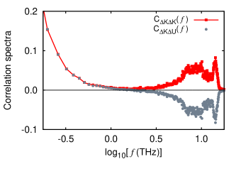
(b)

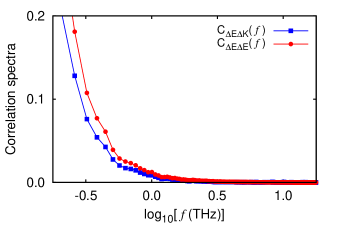
Figure 5: Results of NVT MD simulations with a Langevin thermostat ($\tau_{r}=10$ ps). (a) Comparison of the kinetic energy ACF and kinetic-potential energy CCF in the frequency domain. Note that both spectra have the same shape but opposite sign at high frequencies and coincide at low frequencies. (b) Comparison of the total energy ACF and kinetic-total energy CCF in the frequency domain. Both functions show a similar monotonic decrease with frequency and die off above $1/\tau_{r}$.

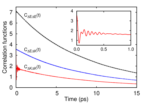
Figure 6: Energy correlation functions in the time domain obtained by NVT MD simulations with a Langevin thermostat ($\tau_{r}=10$ ps). The inset is a zoom into the short-range part of the kinetic energy ACF.

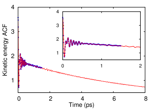
Figure 7: The NVT kinetic energy ACF for a Langevin thermostat with $\tau_{r}=10$ ps (red curve) superimposed on the NVE kinetic energy ACF (blue points). The inset shows a zoom into the short-time region.

IV.3 Additional tests

To demonstrate that the results reported in the previous sections are not artifacts of the Langevin thermostat, selected simulations were repeated using the Nose-Hover thermostat implemented in LAMMPS.(Plimpton, 1995) The results (not shown here for brevity) were found to be in full agreement with the simulations employing the Langevin thermostat, including the timescale separation and validation of the fluctuation relation (1) with temperature computed in quasi-equilibrium states.

Both the Langevin and Nose-Hover algorithms implement virtual thermostats that correctly sample the canonical distribution but still differ from a physical thermostat. The latter is commonly associated with a large volume of some inert substance possessing a large heat capacity and separated from the system by a physical interface. The energy exchange with the thermostat is then controlled by heat conduction across the interface, which is different from random perturbations of atoms uniformly across the system as in the virtual thermostats. To eliminate any possibility that the virtual thermostats could affect our conclusions, efforts were taken to model a “natural” thermostat and show that the conclusions remain valid. By a “natural” thermostat we mean a simulation block much larger than our system and separated from the latter by a physical interface.

As the first step, the NVE MD simulations were executed as above (Sec. IV.1), but this time, atoms within a relatively small cubic block selected at the center of the system were treated as the system itself, whereas the rest of the simulation cell was considered a thermostat. Accordingly, the energy correlation functions were only computed for the small subsystem. Repeating the same statistical analyses as above, it was confirmed that the phonon relaxation time and the thermostat exchange time were significantly different, creating a large time interval (accordingly, a frequency gap in the spectrum of kinetic energy) in which the system existed in quasi-equilibrium states. The temperature defined on this quasi-equilibrium timescale was found to satisfy the fluctuation relation (1).

But even this test was not found completely satisfactory. The volume of the inner lattice block selected as our system was not strictly fixed but rather fluctuated during the simulations. Strictly speaking, the ensemble implemented on the system was NPT (with zero pressure) rather than NVT. Although the fluctuation relations (1) and (2) remain valid in the NPT ensemble as well,(Mishin, 2015) the simulations with the virtual thermostats were conducted in a different (NVT) ensemble.

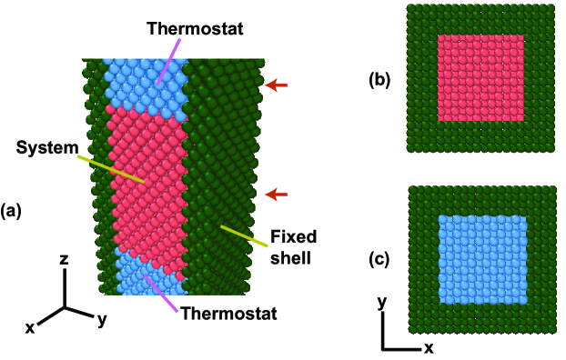
Figure 8: The anatomy of the “natural” thermostat implemented in this work. (a) Vertical cross-section of the simulation block revealing the cubic system under study at the center, the thermostat regions above and below the system, and a fixed shell enclosing both the system and the thermostat. The entire assembly is much longer in the vertical ($z$) direction than shown. (b) and (c) show horizontal ($x$-$y$) cross-sections at the levels indicated by the arrows.

To make sure that the comparison is made for the same ensemble, the natural thermostat was redesigned as shown in Fig. 8. A cubic lattice block with an edge of about 2 nm (about 1400 atoms) was embedded at the center of a larger periodic block with the dimensions $3.6\times 3.6\times 72$ nm (80,000 atoms). This relatively small inner lattice block was the system to be studied. Atoms within a 0.8 nm shell parallel to the long ($z$) direction were fixed in their positions. The remaining atoms above and below the cubic block represented the thermostat and were subject to the following constraint: they could only vibrate in the $x$ and $y$ directions while their $z$-coordinates were fixed. As a result, the cubic system was fully surrounded by atoms incapable of motion in the directions normal to the faces of the cube. The volume of the system was thereby fixed, imitating rigid walls of a calorimeter. At the same time, the thermostat atoms above and below the cube could exchange energy with it by heat conduction across the interfaces mediated by transverse phonons (polarized in the $x$-$y$ plane). This heat exchange controlled the system temperature. The entire assembly was brought to thermal equilibrium at the temperature of 100 K. As usual, the lattice parameter was chosen to ensure zero mechanical stress in the system. Once equilibrium was reached, a 20 ns long NVE MD simulation was performed to compute statistical properties of fluctuations as described above.

Fig. 3(c) shows the normalized differences between the variances/covariances $\langle(\Delta T)^{2}\rangle_{\theta}$, $\langle\Delta E\Delta T\rangle_{\theta}$ and $\langle(\Delta E)^{2}\rangle_{\theta}$ computed with the natural thermostat and the right-hand sides of Eqs.(1), (2) and (3), respectively. The results are qualitatively the same as obtained with the Langevin thermostat [Fig. 3(a,b)]. The deviation from the temperature fluctuation relation (1) is again about 50% when the instantaneous temperature is used ($\theta=dt$) and reduces to approximately $\pm$ 10% when the temperature is defined by the kinetic averaged over the time intervals $\theta\gtrsim 0.1$ ps. When $\theta$ reaches a few ps or higher, the error increases again due to the smoothing of fluctuations by averaging over timescales comparable with the thermostat time. We can conclude that the latter must be on the order of 10 ps. Thus, the quasi-equilibrium timescale for this thermostat is between $\sim 0.1$ and $\sim 10$ ps. In this time interval, the temperature fluctuation relation (1) is approximately followed, although not as accurately as with the Langevin thermostat. This is understandable given that the system in the natural thermostat was a factor of 20 smaller and subject to a size effect. Upscaling of both the system and the thermostat would likely reduce the error but was not pursued in this work.

Spectral analysis of energy fluctuations has shown that the system closely follows the same trends as for the Langevin and Nose-Hoover thermostats. As one example, Fig. 9 compares the power spectra of kinetic energy for the natural and Langevin thermostats. The high-frequency parts of the spectra coincide almost perfectly. The low-frequency parts controlled by energy exchanges with the thermostat also have similar shapes. In fact, for the natural thermostat, this part of the spectrum is very close to that for the Langevin thermostat with $\tau_{r}=10$ ps. This confirms the above estimate of the time constant of the natural thermostat. This also shows that the time constants of the Langevin thermostat chosen for this study were quite realistic. Overall, we can conclude that the association of the temperature fluctuation relation (1) with the quasi-equilibrium timescale has a generic validity and does not reflect some specific features of thermostats.

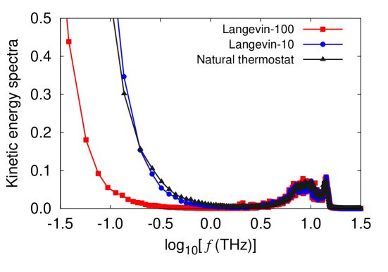
Figure 9: Power spectra of kinetic energy from NVT MD simulations of systems connected to a natural thermostat and two Langevin thermostats with the time constants of 10 and 100 ps.

V Conclusions

We have addressed the long-standing controversy regarding the meaning, or even existence, of temperature fluctuations in canonical systems. Over the past decades, the temperature fluctuation relation (1) appearing in many textbooks and papers(Landau and Lifshitz, 2000; Callen, 1985; Chiu et al., 1992; Mishin, 2015; Hickman and Mishin, 2016) has received different interpretations, including the assertion that this equation is meaningless(Kittel and Kroemer, 2000; Kittel, 1973, 1988) or at best a mere formality.(Mandelbrot, 1989; Falcioni et al., 2011; van Hemmen and Longtin, 2013) We have demonstrated that Eq.(1) is a physically meaningful relation that remains valid as long as the temperature is defined on an appropriate timescale. This interpretation of temperature fluctuations has been supported by MD simulations of a quasi-harmonic solid connected to a thermostat.

The simulations have confirmed the existence of two different fluctuation timescales in canonical systems. The shorter timescale is associated with the time required for a small isolated system to reach thermodynamic equilibrium. For an atomic solid studied here, this time $t_{r}$ is controlled by phonon scattering. In this work, this time was about 0.5 ps at the temperature of 100 K. The longer timescale arises due to slow energy exchanges between the system and the thermostat. Such exchanges may occur by a variety of physically different mechanisms, such as heat transfer across the system/thermostat interface. For the natural and virtual thermostats studied here, the energy exchange time $\tau_{r}$ was on the order of 10 to 100 ps. Thus, $\tau_{r}$ is orders of magnitude longer than $t_{r}$. At the intermediate timescale $t_{q}$ ($t_{r}\ll t_{q}\ll\tau_{r}$) the system remains in internal thermodynamic equilibrium and can be treated as if it were disconnected from the thermostat. In such quasi-equilibrium states, it has well-defined intensive properties such as temperature, pressure and chemical potential.

In particular, temperature can be defined through the equipartition relation using the kinetic energy averaged on the quasi-equilibrium timescale $t_{q}$. It has been shown that fluctuations of the temperature so defined do follow Eq.(1). Attempts to define temperature through kinetic energy averaged over shorter ($<t_{r}$) or longer ($>\tau_{r}$) time intervals result in significant deviations from Eq.(1). In particular, the “temperature” obtained by averaging the kinetic energy over a long time $t\gg\tau_{r}$ does not fluctuate and approaches the thermostat temperature $T$₀.

The timescale separation is also reflected in the shape of the kinetic energy ACF in the frequency domain, showing two peaks separated by a frequency gap. The peak at $f=0$ arises from energy exchanges with the thermostat, whereas the second peak is associated with phonon processes and has the shape of the phonon density of states (plotted against $2f$). The frequency gap represents the quasi-equilibrium states. The potential energy ACF has a similar structure and can also be used for the identification of quasi-equilibrium states. Thus, measured or computed energy spectra of a canonical system carry all information about the timescale on which temperature fluctuations are well-defined and follow Eq.(1).

The conclusions of this work were tested by MD simulations with two virtual thermostats (Langevin and Nose-Hoover) and a natural thermostat consisting of large crystalline regions surrounding the system. In the future, a similar study could evaluate the validity of pressure fluctuation relations for canonical systems.(Landau and Lifshitz, 2000; Rudoi and Sukhanov, 2000; Mishin, 2015)

Acknowledgments - This work was supported by the U.S. Department of Energy, Office of Basic Energy Sciences, Division of Materials Sciences and Engineering, the Physical Behavior of Materials Program, through Grant No. DE-FG02-01ER45871.

References

- Kittel and Kroemer (2000) C. Kittel, H. Kroemer, Thermal physics, second ed., Freeman, W. H. & Company, New York, NY, 2000.
- Kittel (1973) C. Kittel, On the nonexistence of temperature fluctuations in small systems, Am. J. Phys. 41 (1973) 1211–1212.
- Kittel (1988) C. Kittel, Temperature fluctuation: An oxymoron, Phys. Today 41 (1988) 93.
- van Hemmen and Longtin (2013) J. L. van Hemmen, A. Longtin, Temperature fluctuations for a system in contact with a heat bath, J. Statist. Phys. 153 (2013) 1132–1142.
- Chiu et al. (1992) T. C. P. Chiu, D. R. Swanson, M. J. Adriaans, J. A. Nissen, J. A. Lipa, Temperatue fluctuations in the canonical ensemble, Phys. Rev. Lett. 69 (1992) 3005–3009.
- Landau and Lifshitz (2000) L. D. Landau, E. M. Lifshitz, Statistical Physics, Part I, volume 5 of Course of Theoretical Physics, third ed., Butterworth-Heinemann, Oxford, 2000.
- Callen (1985) H. B. Callen, Thermodynamics and an introduciton to thermostatistics, second ed., Wiley, New York, 1985.
- Mishin (2015) Y. Mishin, Thermodynamic theory of equilibrium fluctuations, Annals of Physics 363 (2015) 48–97.
- Mandelbrot (1989) B. B. Mandelbrot, Temperature fluctuations: A well-defined and unavoidable notion, Phys. Today 42 (1989) 71–73.
- Falcioni et al. (2011) M. Falcioni, D. Villamaina, A. Vulpiani, A. Puglisi, A. Sarracino, Estimate of temperature and its uncertainty in small systems, Am. J. Phys. 79 (2011) 777–785.
- Gibbs (1948) J. W. Gibbs, On the equilibrium of heterogeneous substances, in: The collected works of J. W. Gibbs, volume 1, Yale University Press, New Haven, 1948, pp. 55–349.
- De Groot and Mazur (1984) S. R. De Groot, P. Mazur, Non-equilibrium thermodynamics, Dover, New York, 1984.
- Nyquist (1928) H. Nyquist, Thermal agitation of electric charge in conductors, Phys. Rev. 32 (1928).
- Onsager (1931a) L. Onsager, Reciprocal relations in irreversible processes. I, Phys. Rev. 37 (1931a) 405–426.
- Onsager (1931b) L. Onsager, Reciprocal relations in irreversible processes. II, Phys. Rev. 38 (1931b) 2265–2279.
- Callen and Welton (1951) H. B. Callen, T. A. Welton, Irreversibility and generalized noise, Phys. Rev. 83 (1951) 34–40.
- Kubo (1966) R. Kubo, The fluctuation-dissipation theorem, Rep. Prog. Phys. 29 (1966) 255–285.
- Marconi et al. (2008) U. M. B. Marconi, A. Puglisi, L. Rondoni, A. Vulpiani, Fluctuation–dissipation: Response theory in statistical physics, Physics Reports 461 (2008) 111–195.
- Lebowitz et al. (1967) J. L. Lebowitz, J. K. Percus, L. Verlet, Ensemble dependence of fluctuations with application to machine computing, Phys. Rev. 153 (1967) 250–254.
- Mishin et al. (2001) Y. Mishin, M. J. Mehl, D. A. Papaconstantopoulos, A. F. Voter, J. D. Kress, Structural stability and lattice defects in copper: Ab initio, tight-binding and embedded-atom calculations, Phys. Rev. B 63 (2001) 224106.
- Plimpton (1995) S. Plimpton, Fast parallel algorithms for short-range molecular-dynamics, J. Comput. Phys. 117 (1995) 1–19.
- Kong (2011) L. T. Kong, Phonon dispersion measured directly from molecular dynamics simulations, Comp. Phys. Comm. 182 (2011) 2201–2207.
- Frenkel and Smit (2002) D. Frenkel, B. Smit, Understanding molecular simulation: from algorithms to applications, second ed., Academic, San Diego, 2002.
- Kubo et al. (1991) R. Kubo, M. Toda, N. Hashitsume, Statistical Physics II. Nonequilibrium statistical mechanics, volume 31 of Solid-State Sciences, second ed., Springer-Verlag, Berlin, Heidelberg, New York, 1991.
- Dicky and Paskin (1969) J. Dicky, A. Paskin, Computer simulation of the lattice dynamics of solids, Phys. Rev. 188 (1969) 1407–1418.
- Scheidler et al. (2001) P. Scheidler, W. Kob, A. Latz, J. Horbach, K. Binder, Frequency dependent specific heat of viscous silica, Phys. Rev. B 93 (2001) 104204.
- Hickman and Mishin (2016) J. Hickman, Y. Mishin, The energy spectrum of a Langevin oscillator, 2016. To be published. See http://arxiv.org/abs/1607.07467.
- Rudoi and Sukhanov (2000) Y. D. Rudoi, A. D. Sukhanov, Thermodynamic fluctuations within the gibbs and einstein approaches, Phys. Usp. 43 (2000) 1169–1199.