Abstract

In an era of ubiquitous large-scale streaming data, the availability of data far exceeds the capacity of expert human analysts. In many settings, such data is either discarded or stored unprocessed in datacenters. This paper proposes a method of online data thinning, in which large-scale streaming datasets are winnowed to preserve unique, anomalous, or salient elements for timely expert analysis. At the heart of this proposed approach is an online anomaly detection method based on dynamic, low-rank Gaussian mixture models. Specifically, the high-dimensional covariances matrices associated with the Gaussian components are associated with low-rank models. According to this model, most observations lie near a union of subspaces. The low-rank modeling mitigates the curse of dimensionality associated with anomaly detection for high-dimensional data, and recent advances in subspace clustering and subspace tracking allow the proposed method to adapt to dynamic environments. Furthermore, the proposed method allows subsampling, is robust to missing data, and uses a mini-batch online optimization approach. The resulting algorithms are scalable, efficient, and are capable of operating in real time. Experiments on wide-area motion imagery and e-mail databases illustrate the efficacy of the proposed approach.

1 Introduction

Modern sensors are collecting high-dimensional data at unprecedented volume and speed; human analysts cannot keep pace. For instance, many sources of intelligence data must be translated by human experts before they can be widely accessible to analysts and actionable; the translation step is a significant bottleneck [1]. Typical NASA missions collect terabytes of data every day [2, 3, 4, 5]. Incredibly, the Large Hadron Collider (LHC) at CERN “generates so much data that scientists must discard the overwhelming majority of it—hoping hard they’ve not thrown away anything useful.” [6] There is a pressing need to help analysts prioritize data accurately and efficiently from a storage medium or a data stream. This task is complicated by the fact that, typically, the data is neither thoroughly annotated nor meaningfully catalogued. Failure to extract relevant data could lead to incorrect conclusions in the analysis, while extraction of irrelevant data could overwhelm and frustrate human analysts, throttling the discovery process.

This paper focuses on scalable online data processing algorithms that can winnow large datasets to produce smaller subsets of the most important or informative data for human analysts. This process is described as “data thinning.” Often, the data thinning process involves flagging observations which are inconsistent with previous observations from a specified class or category of interest, or are ranked highly according to a learned ranking function. Typically we are interested in methods which can perform these assessments from streaming data, as batch algorithms are inefficient on very large datasets.

One generic approach to the problem of data thinning for large quantities of (possibly streaming) high-dimensional data requires estimating and tracking a probability distribution $f_{t}$ underlying the stream of observations $x_{t}$, and flagging an observation as anomalous whenever $\widehat{f}_{t}(x_{t})<\tau$ for some small threshold $\tau>0$, as demonstrated in past work [7, 8]. Ultimately, the goal is to ensure that the flagged data is salient to human analysts on the receiving end without being buried in an avalanche of irrelevant data. Within this general framework, there are three key challenges:

• Dynamic environments: The data may not be from a stationary distribution. For example, it may exhibit diurnal, location- or weather-dependent patterns. Effective data thinning methods must adapt to those dynamics and sources of bias. Global summary statistics and naive online learning algorithms will fail in this context.

• High-dimensional data: Individual data points $x_{t}$ may be high-dimensional, resulting in the classical “curse of dimensionality” [9, 10]. While large quantities of data may be available, the combination of high-dimensional data and a non-stationary environment still results in an ill-posed estimation problem.

• Real-time processing: In applications like those with NASA and CERN, large quantities of streaming data preclude computationally intensive or batch processing.

1.1 Data thinning for wide-area motion imagery

While our approach is not restricted to imaging data, one important application of our data thinning approach is real-time video analysis. Recent advances in optical engineering have led to the advent of new imaging sensors that collect data at an unprecedented rate and scale; these data often cannot be transmitted efficiently or analyzed by humans due to their sheer volume. For example, the ARGUS system developed by BAE Systems is reported to collect video-rate gigapixel imagery [11, 12], and even higher data rates are anticipated soon [13, 14, 15]. This type of data is often referred to as wide-area motion imagery (WAMI). Currently WAMI streams are used primarily in a forensic context – after a significant event occurs (e.g., a security breach), the data immediately preceding the event are analyzed reactively to piece together what led to that event. However, there is a strong need for predictive analysis which can be used to help anticipate or detect negative events in real time.

Unfortunately, the latter form of analysis is often infeasible for two reasons: (1) the data acquisition rate exceeds the capacity of many sensor platforms’ downlinks; and (2) size, weight, and power constraints limit processing capabilities on airborne sensor platforms. Thus an emerging and fundamental challenge is efficiently downloading salient information to ground-based analysts over a limited-bandwidth channel. While data compression has a long history, conventional compression methods may distort information particularly relevant to analysts. In particular, standard motion imagery compression techniques typically focus on optimizing peak signal-to-noise ratio or psycho-visual metrics which apply globally to an entire video and are often unrelated to any specific task.

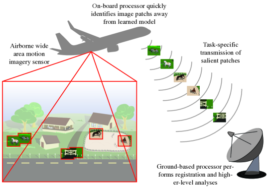
Instead, a better solution would be to identify unique objects or regions of WAMI, and transmit only features of these objects. This concept is illustrated in Fig. 1. Ideally, this method will identify regions and features of a data stream most critical to a given task, and prioritize these features when preparing data for storage or transmission. This task is clearly related to “visual saliency detection” (cf., [16, 17, 18, 19]); we describe the connections between the proposed work and saliency detection in Section 2.

Note that in this setting a key challenge is that the sensor may be placed on a vibrating platform that introduces significant jitter into the data and precludes direct comparison of successive frames. While real-time video stabilization has been considered in the video processing literature (cf., [20, 21, 22, 23, 24]), such methods are often robust for small motions associated with a hand-held device and break down with large motions associated with mechanical vibrations. More robust methods capable of processing larger degrees of jitter can be computationally prohibitive on energy-constrained platforms.

Figure 1: Conceptual illustration of proposed objectives. An airborne platform collects wide-area motion imagery (WAMI), identifies task-specific salient patches, and transmits only those patches. The ground-based receiver can then perform more sophisticated processing, including registration, geolocation, and activity analysis.

1.2 Problem formulation and approach

Suppose we are given a sequence of data $x_{1},x_{2},\ldots,$ and for $t=1,2,\ldots$, $x_{t}\in\mathbb{R}^{p}$, where $p$ denotes the ambient dimension. Assume that $x_{t}$ comes from some unknown distribution, i.e., there exists some sequence of distributions $P_{t}$ such that

$$x_{t}\sim P_{t}\quad t=1,2,\ldots$$

where $P_{t}$ evolves over time, and its distribution density function is denoted by $f_{t}$. The goal is to find the $x_{t}$ that are unusual or anomalous. In particular, we assign each observation $x_{t}$ an anomalousness score proportional to its negative log likelihood under the estimated model—i.e., $-\log f_{t}(x_{t})$. Observations with a low anomalousness score can then either be directed to a human analyst or flagged for further processing and analysis.

The key challenge here is two-fold: (a) the dimension of the signal, $p$, can be quite large, and (b) $f_{t}$ may evolve rapidly over time. The combination of these factors means that our problem is ill-posed, because we are unlikely to gather enough samples to reliably learn the density $f_{t}$.

This paper proposes a method for estimating and tracking the time-series of density functions $f_{t}$ over $\mathbb{R}^{p}$. In stationary, low-dimensional settings, we might consider a Gaussian mixture model that could be estimated, for instance, using an online expectation-maximization (EM) algorithm [25]. However, the non-stationary setting and high dimensions make that approach unviable, as we demonstrate experimentally later in the paper. The proposed approach, by contrast, considers a constrained class of Gaussian mixture models in which the Gaussian covariance matrices (each in the positive-semidefinite cone $\mathcal{S}^{p}_{+}$) are low-rank. This model is equivalent to assuming most $x_{t}$ lie near a union of low-dimensional subspaces. While this union of subspaces is unknown a priori, we may leverage recent advances in subspace tracking (cf., [26, 27, 28, 29]) and subspace clustering (cf., [30, 31, 32, 33, 34, 35]) to yield an accurate sequence of density estimates $\hat{f}_{t}$, and mitigate the curse of dimensionality.

In addition, we consider certain computational and statistical tradeoffs associated with the data thinning problem. In particular, there are two ways to reduce the computational complexity associated with computing anomalousness scores. First, we can reduce the frequency with which we update our model. Second, we can subsample the elements of each $x_{t}$ and leverage missing data models for fast calculations and updates. We demonstrate that these methods, which are not amenable to standard stochastic filtering methods, can yield significant computational speedups with only small decreases in thinning accuracy.

1.3 Contributions and paper layout

This paper presents a data thinning method for high-dimensional streaming data in a dynamic environment. The algorithm adapts to changing environments using tracking methods for union of subspaces. As shown by both synthetic and real-data experiments, the algorithm (a) efficiently tracks the subspaces in which most observation lie and hence precisely detects observations that occur with low probability, and (b) can be applied to a variety of real-world applications and tasks.

Section 2 describes related work. Section 3.1 explains the probability density model based on unions of subspaces, and Section 3 presents the algorithm for tracking such densities. Section 4 describes the computational and statistical tradeoffs associated with the proposed approach. Section 5 reports synthetic experiments which demonstrates the ability of the algorithm to precisely track the density and detect anomalous signals within a changing environment. Section 6, tests the algorithm on the wide-area motion imagery (WAMI) videos to detect salient objects, while Section 7 tests the algorithm on the Enron email database to detect major events.

2 Related work

While data thinning is an emerging concept associated with modern high-dimensional, high-velocity data streams, the formulation described in Section 1.2 is closely related to anomaly detection, visual saliency detection, and subspace clustering and tracking.

2.1 Anomaly detection

The study of anomaly detection has a long and rich history, where the earliest papers can date back to the 19th century [36]. Despite the long history of the study of anomaly detection, most existing detection methods do not work well with high dimensional data, and often do not work online. A 2009 survey on anomaly detection [37] categorizes the available methods into classification-based methods, nearest neighbor-based methods, cluster-based methods, information theoretic methods, statistical anomaly detection methods, and spectral methods.

Among the six categories, classification based methods (cf., [38, 39, 40, 41, 42]) require a large training pool with labeled data that is typically unavailable in the settings of interest. Also, the classification based methods depend highly on the training data, and do not effectively adapt to changing environments. Nearest neighbor (cf., [43, 44, 45, 46, 47]) and cluster-based methods (cf., [48, 49, 50, 51]) can both be extended to work online, but the computational costs are usually high, scaling with the amount of data. Furthermore, the performance of the nearest neighbor and cluster-based methods highly depend on the distance measure, and the optimal distance measure is highly problem-dependent.

Certain statistical methods (cf., [52, 53, 54, 55]) assume that the data are drawn from some standard or predetermined distribution, and determines outliers by computing the likelihood of the signal coming from such distributions. These methods can often work online, and do not rely on a big training set, but estimating the distribution of high-dimensional data is a non-trivial task, and the statistical assumptions do not always hold true, especially for high-dimensional data where there could be spatial correlations.

Information theoretic techniques (cf., [56, 57, 58]) identify the anomalies by trying to find a small subset such that removing the subset will greatly reduce the complexity of the whole set. The approach requires no supervision, and does not make assumptions about the underlying statistical distribution of the data. However, they usually have exponential time complexity and are batch methods. Additionally, it is difficult to assign anomalousness scores to a single data point.

Spectral methods (cf., [59, 60, 61, 62]) assume that data can be embedded into a lower dimensional subspace, and detect anomalies over the embedded space rather than the original space. Because spectral methods essentially operate on a reduced-dimensional representation of the data, they are well-suited to high-dimensional data. Spectral methods can also be integrated with other methods, and are thus highly versatile. However, spectral methods can incur high computational costs; even online anomaly detection algorithms (cf., [63], [64] and [65]) face this challenge. Furthermore, the subspace model underlying spectral methods is less flexible than the union of subspace model underlying this paper’s proposed method.

2.2 Visual saliency detection

In the special case of imagery or video data, data thinning is closely related to visual saliency detection. Like anomaly detection, saliency detection has been widely studied over the last few decades. A standard benchmark for comparison in image saliency detection is proposed by Itti et al. in [16]. This paper attempts to explain human visual search strategies, using biologically motivated algorithms. However, this algorithm is too slow to apply to real time videos. Hou and Zhang in [17] use spectral analysis to detect salient objects for faster speed. However, the analysis breaks down when multiple types of salient objects are present in the scene. Graph-based methods (cf., [18]) work well even when there is no central object in the scene, which is often difficult for other methods to handle, but suffers from high computational complexity. Rao et al. proposed a cluster-based algorithm in [19], where the salient object is identified by first clustering all the pixels according to their local features, and then finding the group of pixels that contains the most salient information. It works better than [16], but not as well as the graph-based algorithms. The information theoretic model based algorithm proposed in [66] claims to work as well as [16], but requires less tuning. This work is improved in [67] for faster speed and better performance.

Methods for image saliency detection have been extended to video saliency detection, but those methods assume a stable imaging platform and video stream free of jitter. In the WAMI application described above, however, sensors can be placed on vibrating platforms that preclude most video saliency detection methods.

2.3 Subspace clustering and tracking

The proposed method is also closely related to the subspace clustering and tracking algorithms. Subspace clustering is a relatively new, but vibrant field of study. These methods cluster observations into low-dimensional subspaces to mitigate the curse of dimensionality, which often make nearest-neighbors-based methods inaccurate [68]. Early works in the field can only identify subspaces that are parallel to the axes, which is not useful when the data is not sparse, but lives on an arbitrarily oriented hyperplane. Newer methods [30, 31, 32, 33, 34, 35], which are also called correlation clustering methods, can identify multiple arbitrarily angled subspaces at the same time, but all share the same problem of high computational cost. Even [35], which is shown to beat other methods in speed, still has an overall complexity of $O(p^{2}T^{2})$, where $p$ is the dimension of the problem, and $T$ is the total number of data points. More recent methods based on sparse modeling (cf., [69, 70, 71, 72, 73]) require solving convex optimization problems that can be inefficient in high-dimensional settings. Thus, the high complexity of the algorithms make them less than ideal candidates for an efficient online algorithm.

Subspace tracking is a classical problem that experienced recent attention with the development of algorithms that are robust to missing and outlier elements of the data points $x_{t}$. For example, the Grassmannian Rank-One Update Subspace Estimation (GROUSE) [26], Parallel Estimation and Tracking by REcursive Least Squares (PETRELS) [27, 28], and Robust Online Subspace Estimation and Tracking Algorithm (ROSETA) [29] effectively track a single subspace using incomplete data vectors. These algorithms are capable of tracking and adapting to changing environments. The subspace model used in these methods, however, is inherently strong, whereas a plethora of empirical studies have demonstrated that high-dimensional data often lie near manifolds with non-negligible curvature [74, 75, 76].

In contrast, the non-parametric mixture of factor analyzers [77] uses a mixture of low-dimensional approximations to fit to unknown and spatially-varying (but static) curvatures. The Multiscale Online Union of SubSpaces Estimation (MOUSSE) method developed by Xie et al. [78] employs union of subspaces tracking for change point detection in high-dimensional streaming data. Thanks to the adoption of the state-of-the-art subspace tracking techniques, the algorithm is both accurate and efficient (with complexity linear in $p$). However, MOUSSE cannot be directly applied for our data thinning task for a few reasons. First, MOUSSE is designed for change-point detection and does not have a probabilistic model. Thus observations in a rare subspace would still be treated as typical, which makes it difficult to discover the rare observations. Second, MOUSSE can only process one observation at a time, i.e., it does not allow for mini-batch updates that can be helpful in data thinning applications, where data could arrive in blocks. Last but not least, although MOUSSE is able to deal with missing data, [78] does not explore the computational-statistical tradeoffs that are important for time- or power-sensitive applications. This paper presents a method that is designed for the data thinning task, has a specific statistical model, and allows for mini-batch updates which increases the algorithm’s efficiency. Also, we will explore the computational-statistical tradeoffs in Section 4.

3 Data thinning via tracking union of subspaces

3.1 Union of subspaces model

Recall from Section 1.2 that each $x_{t}\in\mathbb{R}^{p}$ is assumed to be drawn from a distribution with density $f_{t}$, and that $f_{t}$ is modeled as a mixture of Gaussians where each Gaussian’s covariance matrix is the sum of a rank-$r$ matrix (for $r<p$) and a scaled identity matrix. We refer to this as a dynamic low-rank GMM. In particular, the $j^{\rm th}$ Gaussian mixture component is modeled as

$$\mathcal{N}\left(\mu_{j,t},\Sigma_{j,t}\right)$$

where $\mu_{j,t}\in\mathbb{R}^{p}$ is the mean and

$$\Sigma_{j,t}=V_{j,t}\Lambda_{j,t}V_{j,t}^{T}+\sigma_{j}^{2}I.$$

Here $V_{j,t}\in\mathbb{R}^{p\times r}$ is assumed to have orthonormal columns, and $\Lambda_{j,t}\in\mathbb{R}^{r\times r}$ is a diagonal matrix with positive diagonal entries. If $\sigma_{j}=0$, then $\Sigma_{j,t}$ would be rank-$r$ and any point drawn from that Gaussian would lie within the subspace spanned by the columns of $V_{j,t}$ – shifted by $\mu_{j,t}$. By allowing $\sigma_{j}>0$ we model points drawn from this Gaussian lying near that $r$-dimensional shifted subspace. Overall, we model

$$f_{t}=\sum_{j=1}^{K_{t}}q_{j,t}\mathcal{N}\left(\mu_{j,t},V_{j,t}\Lambda_{j,t}V_{j,t}^{T}+\sigma_{j}^{2}I\right)$$ (1)

where $K_{t}$ is the number of mixture components in the model at time $t$ and $q_{j,t}$ is the probability of $x_{t}$ coming from mixture component $j$.

To better understand this model, we can think of each observation $x_{t}$ as having the form $v_{t}+w_{t}$, where $v_{t}$ lies in a union of subspaces (or more precisely, because of the Gaussian means, a union of hyperplanes) defined by the $V_{j,t}$s and within ellipsoids embedded in those hyperplanes, where the ellipsoid axis lengths are determined by the $\Lambda_{j,t}$s.

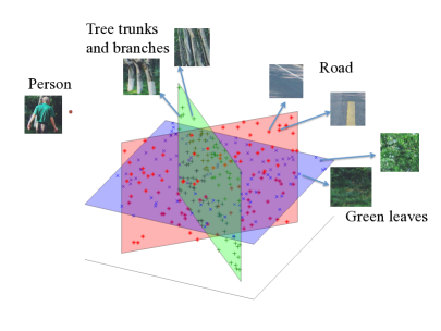
Fig. 2 illustrates the union of subspaces model. Fig. 2a shows a sample image where one person is walking on a road with trees on both sides [79]. In such a situation, we would want to be able to learn from a sequence of such images that the trees, grass and the road which occupy most of the pixels are typical of the background, and label the person as salient because it is uncommon in the scene. Fig. 2b illustrates the union of subspaces model. When we divide the image into patches, the vast majority of patches are plant, and road patches, and only a few patches contain the person. Thus, the plant and road patches live on a union of subspaces as illustrated and can be thinned, leaving anomalous patches for further analysis.

(a) Image of a pedestrian walking on a road with trees on the sides

(b) Illustration of the union of subspaces idea

Figure 2: Illustration of the union of subspaces idea. Fig. 2a shows a pedestrian walking on a road with trees on the sides [79]. The road and the plants occupy most of the pixels, and they can be considered living in a union of subspaces. The person on the road would be considered as an outlier.

3.2 Algorithm highlights

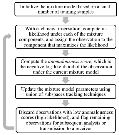
This section explains how the proposed method estimates the evolving Gaussian mixture model using the techniques from the union of subspaces tracking algorithms. These steps are summarized in in Fig. 3. As seen, this data thinning method shares some features with the online EM algorithm for GMM estimation. However, there are a few key differences which are elaborated below:

• We constrain covariances to lie in a union of subspaces, which significantly reduces the problem size for estimating the covariance matrices. This constraint improves the accuracy of the algorithm, and also makes our method much stabler when the environment is changing rapidly relative to the data availability. This constraint also reduces computation time. (More details of computational complexity are discussed in Section 3.5.)

• In some settings, such as when working with WAMI data, we receive groups of $x_{t}$’s simultaneously and can perform model updates more efficiently using mini-batch techniques. (The mini-batch approach is discussed in Section 3.3.3.)

• For large, high-velocity data streams, real-time processing is paramount. Even evaluating the likelihood of each new observation can be time consuming. We explore subsampling-based approximations which reduce computational burden yet still yield accurate results. (Accuracy and computational complexity tradeoffs are discussed in Section 4.)

• For the online EM algorithm for GMM estimation, the number of mixture components is selected a priori, and does not change for the duration of the task. This would work when the environment does not change over time, but is inappropriate for applications that work in dynamic environments. The proposed method adapts to changing numbers of mixture components, which allows the mixture model to better track the environmental dynamics. The method adapts the number of mixture components using a multiscale representation of a hierarchy of subspaces, which allows us to reduce the model order using a simple complexity regularization criterion. The method also tracks hidden subspaces which are then used to increase the model order when data calls for it. (More details about the multi-scale model is discussed in Section 3.3.)

Figure 3: Flow chart of the main steps in the data thinning method.

3.3 The Online Thinning algorithm

This section describes the updates of the parameters associated with the proposed dynamic low-rank GMM in (1). The updates of the mixture component weights ($q_{j,t}$) and means ($\mu_{j,t}$) are computed using stochastic gradient descent. The updates of the covariance matrices are more sophisticated and leverage subspace tracking methods. In particular, we focus on methods which admit observations $x_{t}$ with missing elements; this will allow us to subsample $x_{t}$ for computational speedups. These updates are detailed below.

The biggest challenge is updating $K_{t}$, the number of mixture components. In real-life applications, the number of mixture components is in general (a) not known a priori, and (b) can change with $t$. Thus a mechanism for adaptively choosing the number of subspaces is needed. Reducing model order is slightly less challenging because it is relatively simple to merge two nearby mixture components. However, increasing model order is a much more complex issue, especially in an online setting.

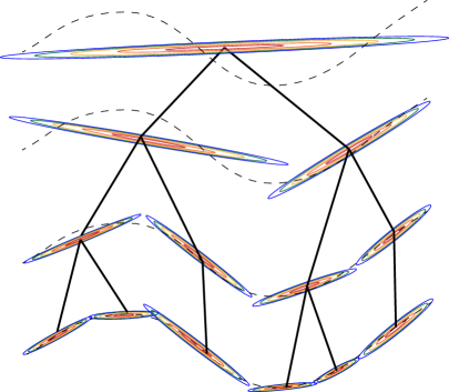
To address these challenges, we organize these mixture components using a tree structure, as illustrated in Fig. 4. The idea for a multiscale tree structure stems from the multiscale harmonic analysis literature [80] and online updates of such models are introduced in [78]. In our setting, at time $t$, the $j^{\mbox{th}}$ node is associated with a Gaussian distribution parameterized by its mean vector $\mu_{j,t}$, low-rank covariance matrix parameters $V_{j,t},\Lambda_{j,t}$, and weight $q_{j,t}$. Most of the probability mass associated with each Gaussian is an ellipsoid centered at $\mu_{j,t}$, where $V_{j,t}$ and $\Lambda_{j,t}$ characterize the principle axes and principal axis lengths, respectively, of the ellipsoid. Finally, $q_{j,t}$ is approximately the probability of an observation falling inside this ellipsoid.

In the tree structure, we denote the set of leaf nodes as $\mathcal{J}_{t}\triangleq\{j:j^{\mbox{th}}\mbox{ node is a leaf node at time }t\}$ and have $K_{t}\triangleq|\mathcal{J}_{t}|$. The leaves of the tree correspond to the Gaussian mixture components in the model shown in Eq. (1). Each parent node corresponds to a single Gaussian which approximates the weighted sum of the Gaussians associated with its two children, where the weights correspond to the children’s $q$ parameters. Each of the tree leaves is also associated with two virtual children nodes. The virtual children nodes correspond to their own Gaussian distributions that can be used to grow the tree. The decision of pruning and growing are made based on (a) the accuracy of the Gaussian mixture model, i.e., the cumulative (with a forgetting factor) anomalousness score, and (b) the size of the mixture model, i.e., the total number of leaf nodes at time $t$.

Figure 4: Multiscale representation of low-rank Gaussian mixture model. Consider a density with its mass concentrated along the black dashed curve. Each successive level in the multiscale representation has more Gaussian mixture components (depicted via contour plots) with covariance matrices corresponding to more compact ellipsoids, and hence yields a more accurate approximation of the underlying density. Given a particular binary tree representation of a GMM, the approximation error can be allowed to increase or decrease by pruning or growing the binary tree connecting the different scales. The ellipsoids are all very compact along some axes because they correspond to covariance matrices that are the sum of a low-rank matrix and a scaled identity matrix.

3.3.1 Computation of the Gaussian mixture likelihood (and anomalousness score)

The proposed algorithm uses the negative log-likelihood of the Gaussian mixture model give the data point as its anomalousness score. The likelihood of $x_{t}$ under the Gaussian associated with node $j$ is given by (recall $\Sigma_{j,t}=V_{j,t}\Lambda_{j,t}V_{j,t}^{T}+\sigma_{j}^{2}I$)

$$p_{j,t}(x_{t})=\frac{1}{(2\pi)^{p/2}|\Sigma_{j,t}|^{1/2}}e^{-\frac{1}{2}(x_{t}-\mu_{j,t})^{T}{\Sigma}_{j,t}^{-1}(x_{t}-\mu_{j,t})}.$$ (2)

Using the model in Eq. (1), the Gaussian mixture negative log-likelihood function (and hence anomalousness score) for any $x_{t}\in\mathbb{R}^{p}$ is:

$$s_{t}(x_{t})= -\log f_{t}(x_{t})$$ (3)

$$= -\log\left(\sum_{j\in\mathcal{J}_{t}}q_{j,t}p_{j,t}(x_{t})\right).$$

3.3.2 Selective update

With the observation of each $x_{t}$, the algorithm first compute the likelihood of $x_{t}$ under each of the Gaussian mixture components, and then assign $x_{t}$ to the component that maximizes the likelihood. Specifically, after the likelihood computations above, $x_{t}$ is assigned to the mixture component

$$j^{*}_{t}\triangleq\arg\max_{j\in\mathcal{J}_{t}}\{p_{j,t}(x_{t})\}.$$ (4)

Note that the weights $q_{j,t}$ are not used here in order to avoid biasing towards components with large weights. This assignment is made in order to reduce the computational complexity of the parameter update step: with each $x_{t}$, instead of updating all the parameters of the entire tree, the algorithm only updates the tree branch associated leaf node $j_{t}^{*}$. That is, the algorithm updates the parameters of node $j_{t}^{*}$, all of its ancestors, and one of node $j_{t}^{*}$’s virtual children (the one under which $x_{t}$ is more likely). This approach significantly reduces the time complexity of the updates, especially when the model is complex (i.e., when the number of leaf nodes is large).

3.3.3 Mini-batch update

In previous sections, we have always assumed that we have one observation $x_{t}\in\mathbb{R}^{p}$ arriving at each time $t$. However, in many applications, multiple observations can arrive simultaneously. For example, in WAMI settings, hundreds of image patches in a single frame arrive at the same time. One way to deal with this is simply treat each patch as arriving at a different time, and update the model parameters separately with each observation. However, when the number of patches is large (for HD videos, there can be thousands of patches per frame), this sequential processing can be extremely time-consuming.

To reduce the computation cost, we can instead update the mixture model in mini-batches, i.e., when multiple observations are received at the same time, we first compute the anomalousness score of each observation, and assign them to their own mixture component. The collection of observations assigned to a given mixture component then form a mini-batch. The mixture model and tree structure are then updated only once for each mini-batch. When the size of mini-batches is much larger than 1 (e.g., hundreds of image patches assigned to a tree of size $K_{t}=10$), this approach significantly reduces the number of times needed to update the mixture component parameters and tree structures, and thus saves computation time. Note that this mini-batch processing does not affect the computation of the anomalousness score and component assignment, where each observation is processed sequentially as if they arrive separately.

Thus, now instead of assuming a single vector $x_{t}$ arrives at time $t$, we assume that we receive a collection of observations stored in matrix $X_{t}=[x_{t,1},\ldots,x_{t,N_{t}}]\in\mathbb{R}^{p\times N_{t}}$ at time $t$, where $x_{t,i}\in\mathbb{R}^{p}$ for all $i=1,\ldots,N_{t}$. A special case of this is $N_{t}=1$, which is the sequential update without mini-batches. After assigning each column in $X_{t}$ to the $K_{t}$ leaf nodes in the hierarchical tree structure based on their distance to the corresponding mixture components, we can rewrite $X_{t}$ into mini-batches, $X_{t}=[X_{j_{1},t},\cdots,X_{j_{K_{t}},t}]$, where $\{j_{1},\ldots,j_{K_{t}}\}\subseteq\mathcal{J}_{t}$. Here each $X_{j_{i},t}\in\mathbb{R}^{p\times n_{j,t}},i=1,\ldots,K_{t}$ is a block of $n_{j,t}$ data points that are assigned to the $j_{i}^{\mbox{th}}$ node in the tree (must be a leaf node). Note that $\sum_{j\in\mathcal{J}_{t}}n_{j,t}=N_{t}$.

Our update equations are based on a “forgetting factor” $\alpha\in(0,1)$ that places more weight on more recent observations; this quantity affects how quickly a changing distribution is tracked and is considered a tuning parameter to be set by the end user. Then for each leaf node $j$ that needs updates (i.e., with assigned observations), the weights $q_{j,t}$ are then updated by

$$q_{j,t+1}=\alpha q_{j,t}+(1-\alpha)\frac{n_{j,t}}{N_{t}}.$$ (5)

Note that for the leaf nodes the weights need to add to 1, i.e., $\sum_{j\in\mathcal{J}_{t}}q_{j,t}=1$ for all $t$. If we initialize $q_{j,1}$ s.t. $\sum_{i\in\mathcal{J}_{1}}q_{j,1}=1$ , and the weight of any parent node is the sum of the weights of its two children, then this update preserves $\sum_{i\in\mathcal{J}_{t}}q_{j,t}=1$ for all $t$. The mixture component means $\mu_{j,t}$ are updated by

$$\mu_{j,t+1}=\alpha\mu_{j,t}+\frac{(1-\alpha)}{n_{j,t}}X_{j,t}\mathbbm{1}_{n_{j,t}\times 1}.$$ (6)

The diagonal matrix

$${\Lambda}_{j,t}\triangleq\mbox{diag}\{\lambda_{j,t}^{(1)},\ldots,\lambda_{j,t}^{(r)}\}\in\mathbb{R}^{r\times r},$$

with $\lambda_{j,t}^{(1)},\ldots,\lambda_{j,t}^{(r)}\geq 0$, contains eigenvalues of the covariance matrix of the projected data onto each subspace. Let

$$M_{j,t}=[\mu_{j,t},\ldots,\mu_{j,t}]\in\mathbb{R}^{p\times n_{j,t}}$$ (7)

be a means matrix computed by concatenating $n_{j,t}$ copies of $\mu_{j,t}$ together. Let

$$B_{j,t}=V_{j,t}^{\#}(X_{j,t}-M_{j,t}),$$ (8)

be the residual signal, where the superscript ^# denotes the pseudo-inverse of a matrix (for orthonormal $V_{j,t}$, the pseudo-inverse is its transpose). Denote its $m^{\mbox{th}}$ row as $B_{j,t}^{(m)}$. Then we can update

$$\lambda_{j,t+1}^{(m)}=\alpha\lambda_{j,t}^{(m)}+(1-\alpha)\|B_{j,t}^{(m)}\|_{2}^{2},m=1,\ldots,r.$$ (9)

The subspace matrices $V_{j,t}$ are updated using Algorithm. 1. The updates of $V_{j,t}$ and $\Lambda_{j,t}$ are a mini-batch extension of the PETRELS [28, 27] update equations, with an added step of orthonormalization of $V_{j,t+1}$ since PETRELS does not guarantee the orthogonality of $V_{j,t+1}$.

For the ancestors of each leaf node that got updated, we combine all the mini-batches assigned to its children, and update the node with the same formulae as above using the combined mini-batches. For the virtual children of leaf nodes that got updated, we divide each mini-batch into two sub-mini-batches based on the likelihood of each observation under the Gaussian of the virtual node, and update each virtual node with its assigned sub-mini-batch.

Algorithm 1 Mini-Batch Update of Covariance Parameters

1:Initialize: $V_{j,1}$ (with training data), $R_{j,1}=c\mathbbm{1}_{r\times r},c\ll 1$

2:input: $X_{j,t},V_{j,t},R_{j,t},M_{j,t}$

3:$B_{j,t}=V_{j,t}^{\#}(X_{j,t}-M_{j,t})$

4:$R_{j,t+1}=\alpha R_{j,t}+B_{j,t}B_{j,t}^{T}$

5:${\widetilde{V}}_{j,t+1}={V}_{j,t}+\left((X_{j,t}-M_{j,t})B_{j,t}^{T}-V_{j,t}B_{j,t}B_{j,t}^{T}\right)R_{j,t+1}^{\#}$

6:Orthonormalization

7: ${V}_{j,t+1}={\widetilde{V}}_{j,t+1}\left({\widetilde{V}}_{j,t+1}^{T}{\widetilde{V}}_{j,t+1}\right)^{-\frac{1}{2}}$

8:Output: $V_{j,t+1},R_{j,t+1}$

3.3.4 Tree structure update

The growing (splitting nodes) and pruning (merging nodes) of the tree structure allow the complexity of the GMM to adapt to the diversity of the observed data. The number of nodes in the tree controls the tradeoff between the model accuracy and complexity. The proposed method determines whether to grow or prune the tree by greedily minimizing a cost function consisting of the weighted cumulative anomalousness score (with weights corresponding to the forgetting factor $\alpha$ described above) and the model complexity ($|\mathcal{J}_{t}|$).

Define $\epsilon_{t}$ as the cumulative anomalousness score where $\epsilon_{0}=0$, and

$$\epsilon_{t+1}=\alpha\epsilon_{t}+\frac{1}{N_{t}}\sum_{i=1}^{N_{t}}s_{t}(x_{t,i}).$$

For each node $j$ (including virtual children), a similar cumulative score $e_{j,t}$ is kept based only on the mini-batches assigned to that node. Let $\mathcal{I}_{j,t}\triangleq\{i:x_{t,i}\mbox{ assigned to }j^{\mbox{th}}\mbox{ node or its children}\}$ (for virtual nodes this set is the indices of its sub-mini-batch), initialize $e_{j,0}=0$, and $e_{j,t}$ is updated by

$$e_{j,t+1}=\alpha e_{j,t}+\frac{1}{|\mathcal{I}_{j,t}|}\sum_{i\in\mathcal{I}_{j,t}}-\log\left(p_{j,t}(x_{t,i})\right).$$

Let tol be a pre-set error tolerance. For each leaf node $j_{1}\in\mathcal{J}_{t}$ that is assigned new observations, let $j_{0}$ be its parent, $j_{2}$ be its sibling, and $j_{1,1},j_{1,2}$ be its virtual children. Let $\gamma$ be a positive constant. Split node $j_{1}$ if

$$\epsilon_{t+1}\leq{\mbox{\sc tol}},$$ (10)

and

$$e_{j_{1},t}+\gamma K_{t}>\frac{q_{j_{1,1},t}e_{j_{1,1},t}+q_{j_{1,2},t}e_{j_{1,2},t}}{q_{j_{1,1},t}+q_{j_{1,2},t}}+\gamma(K_{t}+1).$$ (11)

Note the left side of Ineq. (11) is the penalized cumulative score of node $j_{1}$ (where the penalty is proportional to the number of nodes in the tree), while the right side of Eq. (11) is the average penalized cumulative score of node $j_{1}$’s two virtual children. We split node $j_{1}$ if the average penalized cumulative score is smaller at the virtual children level.

Similarly, merge nodes $j_{1}$ and $j_{2}$ if

$$\epsilon_{t+1}\geq{\mbox{\sc tol}}$$ (12)

and

$$e_{j_{0},t}+\gamma(K_{t}-1)<\frac{q_{j_{1},t}e_{j_{1},t}+q_{j_{2},t}e_{j_{2},t}}{q_{j_{1},t}+q_{j_{2},t}}+\gamma K_{t},$$ (13)

Note the left side of Ineq. (13) is the penalized (with tree size) cumulative score of node $j_{1}$’s parent $j_{0}$, while the right side of Eq. (11) is the average penalized cumulative score of node $j_{1}$ and its sibling $j_{2}$. We merge $j_{1}$ and $j_{2}$ if the average penalized cumulative score of $j_{1}$ and $j_{1}$ is larger than the penalized score of their parent. The use of these penalized scores to choose a tree which is both (a) a good fit to the observed data and (b) a small as possible to avoid overfitting is common in classification and regression trees [81, 82, 83, 84, 85, 86]. The splitting and merging operations are detailed in Algorithm 2 and Algorithm 3. The complete Online Thinning algorithm is summarized in Algorithm 4.

Algorithm 2 Grow tree

1:Input: Node $j$ with virtual children nodes $k$ and $\ell$

2:Update $\mathcal{J}_{t+1}=\mathcal{J}_{t}\bigcup\{k,\ell\}\backslash\{j\}$

3:Create new virtual children: $k_{1},k_{2}$ for new leaf node $k$, and $j_{1,1},j_{1,2}$ for new leaf node $\ell$

4:Let $v_{i,t}^{(1)}$ be the first column of $V_{i,t},i\in\{k,\ell\}$

5:Initialize virtual nodes $k_{1},k_{2},j_{1,1}$ and $j_{1,2}$:

6: for $i\in\{k,\ell\}$

$$\mu_{i_{1},t+1} =\mu_{i,t}+\sqrt{\lambda_{i,t}^{(1)}}v^{(1)}_{i,t}/2$$

$$\mu_{i_{2},t+1} =\mu_{i,t}-\sqrt{\lambda_{i,t}^{(1)}}v^{(1)}_{i,t}/2$$

$$V_{i_{1},t+1} =V_{i,t}$$

$$V_{i_{2},t+1} =V_{i,t}$$

$$\lambda_{i_{1},t+1}^{(1)} =\lambda_{i,t}^{(1)}/2$$

$$\lambda_{i_{2},t+1}^{(1)} =\lambda_{i,t}^{(1)}/2$$

$$\lambda_{i_{1},t+1}^{(m)} =\lambda_{j,t}^{(m)},\quad m=2,\ldots,r$$

$$\lambda_{i_{2},t+1}^{(m)} =\lambda_{j,t}^{(m)},\quad m=2,\ldots,r$$

$$q_{i_{1},t+1} =q_{j,t}/2$$

$$q_{i_{2},t+1} =q_{j,t}/2$$

Algorithm 3 Prune tree

1:Input: Node $j$ with children nodes $j_{1}$ and $j_{2}$ to be merged

2:Delete all four virtual children nodes of $j_{1}$ and $j_{2}$

3:Update $\mathcal{J}_{t+1}=\mathcal{J}_{t}\bigcup\{j\}\backslash\{j_{1},j_{2}\}$

4:Define $j_{1}$, $j_{2}$ as the virtual children nodes of the new leaf node $j$

Algorithm 4 Online Thinning with Mini-Batch Updates

1:input: error tolerance ${\mbox{\sc tol}}>0$, threshold $\tau>0$, forgetting factor $\alpha\in(0,1)$

2:initialize: tree structure, set initial error $\epsilon_{1}=0$

3:for $t=1,2,\ldots$ do

4:     receive new data $X_{t}\in\mathbb{R}^{p\times N_{t}}$

5:     for $i=1,2,\ldots,N_{t}$ do

6:         let $x_{t,i}$ be the $i^{\mbox{th}}$ column of $X_{t}$

7:         for all $j\in\mathcal{J}_{t}$, compute likelihood of $x_{t,i}$ under node $j$:

$$p_{j,t}(x_{t,i})=\frac{1}{(2\pi)^{p/2}|\Sigma_{j,t}|^{1/2}}e^{-\frac{1}{2}(x_{t,i}-\mu_{j,t})^{T}{\Sigma}_{j,t}^{-1}(x_{t,i}-\mu_{j,t})}$$

8:         compute anomalousness score $s_{t}(x_{t,i})$:

$$s_{t}(x_{t,i})=-\log\left(\sum_{j\in\mathcal{J}_{t}}q_{j,t}p_{j,t}(x_{t,i})\right)$$

9:         assign $x_{t,i}$ to leaf node $j^{*}_{t}\triangleq\arg\max_{j\in\mathcal{J}_{t}}\{p_{j,t}(x_{t,i})\}.$

10:         compute the likelihood of $x_{t,i}$ under $j^{*}$’s two virtual children nodes, and also assign $x_{t,i}$ to the virtual child with higher likelihood

11:     end for

12:     update $\epsilon_{t+1}=\alpha\epsilon_{t}+\frac{1}{N_{t}}\sum_{i=1}^{N_{t}}s_{t}(x_{t,i})$

13:     for  all nodes $j$ in the tree do

14:         set $\mathcal{I}_{j,t}\triangleq\{i:x_{t,i}\mbox{ assigned to }j^{\mbox{th}}\mbox{ node or its children}\}$

15:         if $\mathcal{I}_{j,t}$ is not empty then

16:              denote all data assigned to node $j$ or its children as $X_{j,t}=[x_{1},\ldots,x_{n_{j,t}}]$

17:              update $e_{j,t+1}=\alpha e_{j,t}+\frac{1}{|\mathcal{I}_{j,t}|}\sum_{i\in\mathcal{I}_{j,t}}-\log\left(p_{j,t}(x_{t,i})\right)$

18:              update $q_{j,t+1}=\alpha q_{j,t}+(1-\alpha)\frac{n_{j,t}}{N_{t}}$

19:              update $\mu_{j,t+1}=\alpha\mu_{j,t}+\frac{(1-\alpha)}{n_{j,t}}X_{j,t}\mathbbm{1}_{n_{j,t}\times 1}$

20:              set $M_{j,t}=[\mu_{j,t},\ldots,\mu_{j,t}]\in\mathbb{R}^{p\times n_{j,t}}$

21:              set $B_{j,t}=V_{j,t}^{\#}(X_{j,t}-M_{j,t})$

22:              for $m=1,\ldots,r$ do

23:                  update $\lambda_{j,t+1}^{(m)}=\alpha\lambda_{j,t}^{(m)}+(1-\alpha)\|B_{j,t}^{(m)}\|_{2}^{2}$

24:              end for

25:              update $V_{j,t}$ by calling Algorithm 1

26:              if $\epsilon_{t+1}\leq{\mbox{\sc tol}}$ and $e_{j_{1},t}+\gamma K_{t}>\frac{q_{j_{1,1},t}e_{j_{1,1},t}+q_{j_{1,2},t}e_{j_{1,2},t}}{q_{j_{1,1},t}+q_{j_{1,2},t}}+\gamma(K_{t}+1)$ then

27:                  call Algorithm 2

28:              else if $\epsilon_{t+1}\geq{\mbox{\sc tol}}$ and $e_{j_{0},t}+\gamma(K_{t}-1)<\frac{q_{j_{1},t}e_{j_{1},t}+q_{j_{2},t}e_{j_{2},t}}{q_{j_{1},t}+q_{j_{2},t}}+\gamma K_{t}$ then

29:                  call Algorithm 3

30:              end if

31:         else update $q_{j,t+1}=\alpha q_{j,t}$

32:         end if

33:     end for

34:     $\mathcal{X}_{t}=\{x_{t,i}:s_{t}(x_{t,i})>\tau\}$

35:end for

36:output: sequence of thinned data $\mathcal{X}_{1},\ldots,\mathcal{X}_{T}$

3.4 Subsampling observations

When $p$ is large and computation time is critical, we can subsample the elements of each $X_{t}$ and leverage missing data models for fast calculations and updates. Algorithm 1 is a modified version of PETRELS [27, 28] with mini-batches. Note that PETRELS was specifically designed to work with missing entries, where [27, 28] thoroughly investigated the effect of missing data in subspace tracking algorithms.

Specifically, to modify our Online Thinning algorithm for $X_{t}$ with subsampled entries, we define $\Omega_{t}\subseteq\{1,\ldots,p\}$ be the subset of entries used at time $t$. Assume all $\Omega_{t}$ have the same size and define $|\Omega|\triangleq|\Omega_{t}|,\forall t$. Define an operator $P_{\Omega_{t}}(\cdot)$ that selects the rows indexed by $\Omega_{t}$. Then, for the likelihood and score computation, denote $\Sigma_{j,t,\Omega_{t}}\triangleq P_{\Omega_{t}}(V_{j,t})\Lambda_{j,t}P_{\Omega_{t}}(V_{j,t})^{T}+\sigma_{j}^{2}I_{|\Omega_{t}|}$, and compute

$$p_{j,t}(x_{t}) =\frac{1}{(2\pi)^{p/2}|\Sigma_{j,t}|^{1/2}}\exp\left\{-\frac{1}{2}\left[P_{\Omega_{t}}(x_{t,i})\right.\right.$$

$$\left.\left.-P_{\Omega_{t}}(\mu_{j,t})\right]^{T}{\Sigma}_{j,t,\Omega_{t}}^{-1}\left[P_{\Omega_{t}}(x_{t,i})-P_{\Omega_{t}}(\mu_{j,t})\right]\right\}$$

as the likelihood. For the mini-batch update step, replace $X_{j,t},\mu_{j,t},$ and $V_{j,t}$ with $P_{\Omega_{t}}(X_{j,t}),P_{\Omega_{t}}(\mu_{j,t}),$ and $P_{\Omega_{t}}(V_{j,t})$, respectively in Eq. (6),(7), and (8), and use Algorithm 5 instead of Algorithm 1.

Algorithm 5 Mini-Batch Update of Covariance Parameters with Subsampling

1:Initialize: $V_{j,1}$ (with training data), $R_{j,1}=c\mathbbm{1}_{r\times r},c\ll 1$

2:input: $\Omega_{t},P_{\Omega_{t}}(X_{j,t}),V_{j,t},R_{j,t},P_{\Omega_{t}}(M_{j,t})$

3:$B_{j,t}=P_{\Omega_{t}}(V_{j,t})^{\#}\left[P_{\Omega_{t}}(X_{j,t})-P_{\Omega_{t}}(M_{j,t})\right]$

4:$R_{j,t+1}=\alpha R_{j,t}+B_{j,t}B_{j,t}^{T}$

5:${\widetilde{V}}_{j,t+1}={V}_{j,t}$

6:$P_{\Omega_{t}}({\widetilde{V}}_{j,t+1})=P_{\Omega_{t}}({\widetilde{V}}_{j,t+1})+\left[(P_{\Omega_{t}}(X_{j,t})\right.$

7:$\left.-P_{\Omega_{t}}(M_{j,t}))B_{j,t}^{T}-P_{\Omega_{t}}(V_{j,t})B_{j,t}B_{j,t}^{T}\right]R_{j,t+1}^{\#}$

8:Orthonormalization

9: ${V}_{j,t+1}={\widetilde{V}}_{j,t+1}\left({\widetilde{V}}_{j,t+1}^{T}{\widetilde{V}}_{j,t+1}\right)^{-\frac{1}{2}}$

10:Output: $V_{j,t+1},R_{j,t+1}$

3.5 Computational complexity

As discussed in Section 3, the union of subspaces assumption significantly reduces the problem size for estimating the covariance matrices. This not only improves the algorithm accuracy and stability for high dimensional problems, but also reduces computation time.

Take the computation of $(x-\mu_{j,t})^{T}\Sigma_{j,t}^{-1}(x-\mu_{j,t})$ as an example. $\Sigma_{j,t}$ is the covariance matrix of the $j^{\mbox{th}}$ mixture component at time $t$. For a full-rank GMM model, computing the $\Sigma_{j,t}^{-1}$ takes $O(p^{3})$ operations, and computing $(x-\mu_{j,t})^{T}\Sigma_{j,t}^{-1}(x-\mu_{j,t})$ given $\Sigma_{j,t}^{-1}$ takes $O(p^{2})$ operations. Thus the total complexity is $O(p^{3})$. However, with the low-rank assumption we have $\Sigma_{j,t}=V_{j,t}\Lambda_{j,t}V_{j,t}^{T}+\sigma^{2}I$, and with the Woodbury matrix identity [87], we can compute

$$\Sigma_{j,t}^{-1}=\sigma^{-2}I+\sigma^{-4}V_{j,t}(\Lambda_{j,t}^{-1}+V_{j,t}^{T}V_{j,t})^{-1}V_{j,t}^{T},$$

and

$$(x-\mu_{j,t})^{T}\Sigma_{j,t}^{-1}(x-\mu_{j,t})=$$

$$\sigma^{-2}(x-\mu_{j,t})^{T}(x-\mu_{j,t})$$

$$+\sigma^{-4}(x-\mu_{j,t})^{T}V_{j,t}(\Lambda_{j,t}^{-1}+V_{j,t}^{T}V_{j,t})^{-1}V_{j,t}^{T}(x-\mu_{j,t}).$$

Note that computing $(\Lambda_{j,t}^{-1}+V_{j,t}^{T}V_{j,t})^{-1}$ is easy because (a) $V_{j,t}^{T}V_{j,t}=I_{r}$ since the columns of $V_{j,t}$ are orthonormal, and (b) $\Lambda_{j,t}$ is diagonal. Computing the whole equation takes $O(pr+r^{2})=O(pr)$ operations. Thus, by using the low-dimensional structure, we reduced the computation complexity from $O(p^{3})$ to $O(pr)$.

Another example is the computation of the determinant of $\Sigma_{j,t}$. For a full-rank GMM model, computing $|\Sigma_{j,t}|$ takes $O(p^{3})$ operations. For our low-rank model with $\Sigma_{j,t}=V_{j,t}\Lambda_{j,t}V_{j,t}^{T}+\sigma^{2}I$, we can use the matrix determinant lemma [88] and compute

$$|\Sigma_{j,t}| =\sigma^{2}\left|\Lambda_{j,t}\right|\left|\Lambda_{j,t}^{-1}+\sigma^{-2}V_{j,t}^{T}V_{j,t}\right|.$$

The number of operation needed is O(r) since $V_{j,t}^{T}V_{j,t}=I_{r}$ and $\Lambda_{j,t}$ is diagonal.

3.5.1 Computational complexity without subsampling

Below we summarize the computational complexity of each major steps of the Online Thinning algorithm.Let $T$ be the total number of time steps. For simplicity, we assume the mini-batch sizes $N_{t}$ are the same for all $t$. Let $N\triangleq TN_{t}$ be the total number of observations received, and $K_{\mbox{max}}$ be the maximum number of leaf nodes in the tree.

• Likelihood and score computation has a complexity of

  $$O(NK_{\mbox{max}}pr),$$

  where each likelihood computation takes $O(pr)$ operations, and this is computed $K_{\mbox{max}}+2$ times per observation ($K_{\mbox{max}}$ leaf nodes plus two virtual children of the assigned leaf node) for all $N$ observations. The computation of the anomalousness score is computationally inexpensive since it is a weighted sum of pre-computed likelihoods.

• Mini-batch updates have complexities of at most

  $$O\left(NK_{\mbox{max}}pr+\frac{N}{N_{t}}K_{\mbox{max}}pr^{2}\right),$$

  where the first term $NK_{\mbox{max}}pr$ comes from the calculation of $B_{j,t}$ and ${\widetilde{V}}_{j,t+1}$, and the second term comes from the orthonormalization of ${\widetilde{V}}_{j,t+1}$. The term $\frac{N}{N_{t}}$ is the number of batches received.

• Tree structure updates have complexities of at most

  $$O(NK_{\mbox{max}}pr+\frac{N}{N_{t}}K_{\mbox{max}}pr),$$

  where the first term is an upper bound of complexity for updating the cumulative likelihood $e_{j,t}$ of the parents of leaf nodes (for leaf nodes and their virtual children, the likelihood is computed when at the score computing stage). In the second term, the term $pr$ comes from the number of operations needed to copy the subspace when splitting nodes, and the maximum number of splitting at each time $t$ is bounded by the maximum number of leaf nodes $K_{\mbox{max}}$ (merging nodes is computational inexpensive).

Adding three steps together, the Online Thinning algorithm has a complexity of at most

$$O\left(NK_{\mbox{max}}pr+\frac{N}{N_{t}}K_{\mbox{max}}pr^{2}\right).$$

3.5.2 Computational complexity with subsampling

Let $|\Omega|$ be the number of entries observed after subsampling, then the complexity of each major step is as follows.

• Likelihood and score computation has a complexity of

  $$O(NK_{\mbox{max}}|\Omega|r),$$

  which scales with $|\Omega|$.

• Mini-batch updates have complexities of at most

  $$O\left(NK_{\mbox{max}}(|\Omega|r+r^{2})+\frac{N}{N_{t}}K_{\mbox{max}}pr^{2}\right),$$

  where the first term $NK_{\mbox{max}}(|\Omega|r+r^{2})$ comes from the calculation of $B_{j,t}$ and ${\widetilde{V}}_{j,t+1}$, and is affected by subsampling. Note the extra $NK_{\mbox{max}}r^{2}$ comes from the added complexity from computing $P_{\Omega_{t}}(V_{j,t})^{\#}$. When no subsampling is done, $V_{j,t}^{\#}=V_{j,t}^{T}$. However, this is generally not true when we perform subsampling, and this extra step adds complexity. However, in general $|\Omega|$ scales with $p$ and is much larger than $r$. The second term comes from the orthonormalization of ${\widetilde{V}}_{j,t+1}$, which is not affected by subsampling.

• Tree structure updates have complexities of at most

  $$O(NK_{\mbox{max}}|\Omega|r+\frac{N}{N_{t}}K_{\mbox{max}}pr),$$

  where the first term comes from the likelihood computation, and scales with $|\Omega|$. The second comes from the tree splitting, which is not affected by subsampling.

Adding three steps together, the Online Thinning algorithm has a complexity of at most

$$O\left(NK_{\mbox{max}}(|\Omega|r+r^{2})+\frac{N}{N_{t}}K_{\mbox{max}}pr^{2}\right).$$

3.5.3 Remarks

Subsampling changes the first term of the complexity. Higher subsampling rates (smaller $|\Omega|$) reduce the complexity of computing the likelihood, and affect some steps in the mini-batch update. However, subsampling does not affect the orthonormalization of $V_{j,t}$, or the splitting and merging of tree structures. Additionally, subsampling makes the computation of $P_{\Omega_{t}}(V_{j,t})^{\#}$ difficult, since in general $P_{\Omega_{t}}(V_{j,t})^{\#}\neq P_{\Omega_{t}}(V_{j,t})^{T}$. Still, the effect of this added complexity in computing $P_{\Omega_{t}}(V_{j,t})^{\#}$ is generally small since $|\Omega|$ is usually much larger than $r$.

Changing the size of mini-batches $N_{t}$ changes $\frac{N}{N_{t}}$, and thus the second term of the complexity. Specifically, in the algorithm, changing $N_{t}$ changes (a) the number of times needed to update the tree structure, (b) the number of times needed to update $R_{j,t}$ and its pseudo-inverse (see Algorithm 1), and (c) the number of time needed to perform the orthonormalization of $V_{j,t}$ (see Algorithm 1). When $N_{t}$ has the same order of (or larger than) $K_{\mbox{max}}r$, and without subsampling, the algorithm’s complexity is linear to the total number of observations $N$, the observation dimension $p$, the tree size $K_{\mbox{max}}$, and the subspace dimension $r$.

4 Computational and statistical tradeoffs

Different systems have different delay allowances and precision requirements, and it is natural to ask how much performance we sacrifice by trying to reduce the computation time. Understanding such tradeoffs is crucial for applications where real-time processing is required, yet the computational power is limited, as with many mobile surveillance systems. This section explores the tradeoff between processing time and detection accuracy for the Online Thinning algorithm.

There are two primary ways to reduce the computational complexity of the data thinning: (1) by randomly subsampling the entries of $x_{t}$, i.e., we only use partially observed data to update the dynamic low-rank GMM model parameters and estimate the anomalousness score; and (2) by varying the size of the mini-batches. Note that these are made possible because, as discussed in Section 3, data thinning (a) is robust to unobserved entries, and (b) can process data in mini-batches, respectively.

To explore this further, two experiments are conducted—one in which we vary the mini-batch size, and one in which we vary the subsampling rate. For these experiments, the data is generated as follows: The ambient dimension is $p=100$. We first generate points in $\mathbb{R}^{p}$ in a union of three (shifted) subspaces of dimension ten; in which 95% of the points lie in the union of the first two subspaces. The other 5% of the points lie in a third subspace that is orthogonal to the other two. All three subspaces have shifts close to 0. We then add white Gaussian noise with variance $\sigma^{2}=0.1$ to these points to generate our observations. The two subspaces where the 95% of observations come from are dynamic, where the subspaces rotate at a speed $\delta>0$. For $j=1,2$, we have

$$V_{j,t+1}=V_{j,t}+\delta\frac{B}{\|B\|_{F}}V_{j,t},$$

where $B$ is a $p\times p$ skew-symmetric matrix. Denote the set of $x_{t}$’s coming from each of the three subspaces as $\mathcal{X}_{j},j=1,2,3$, respectively. The goal is to identify the 5% of the observations that come from $\mathcal{X}_{3}$.

The experiment streams in four thousand observations in total. An initial model is estimated using the first one thousand samples, and the models are then updated in an online fashion for the remaining three thousand samples. The anomalousness score is calculated as the negative log-likelihood of each data point according to the estimated model. We then select observations $x_{t}$ for which $s_{t}(x_{t})>\tau$, and compute the detection rate and false alarm rate

$$P_{D}(\tau)=\frac{|\{t:x_{t}\in\mathcal{X}_{3},s_{t}(x_{t})>\tau\}|}{|\{t:x_{t}\in\mathcal{X}_{3}\}|},$$

$$P_{F}(\tau)=\frac{|\{t:x_{t}\in\mathcal{X}_{1}\bigcup\mathcal{X}_{2},s_{t}(x_{t})>\tau\}|}{|\{t:x_{t}\in\mathcal{X}_{1}\bigcup\mathcal{X}_{2}\}|}.$$

The threshold $\tau$ is tuned to minimize the detection error $1-P_{D}(\tau)+P_{F}(\tau)$. Each experiment is averaged over ten random realizations.

The first experiment varies the percentage of entries observed in each $x_{t}$. Subsampling reduces the dimension of $x_{t}$, which saves time in many of the operations in the algorithm. With more observed entries, the estimates of the likelihoods under each mixture component are more accurate, and hence the thinning performance is better. However, the computation of likelihoods and updates of the dynamic low-rank GMM parameters will also be slower.

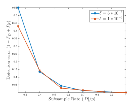
Fig. 5 shows the detection error of our approach as a function of subsampling rate ($|\Omega|/p$). The two curves correspond to different subspace rotation speed ($\delta$). We vary the subsampling rate from 25% to 100%. The detection error is kept at less than 5% even at a subsampling rate of 55%.

Figure 5: Detection error as a function of subsampling rate. The two curves correspond to different subspace rotation speed ($\delta$). A subsampling rate at 55% still keeps the detection error less than 5%.

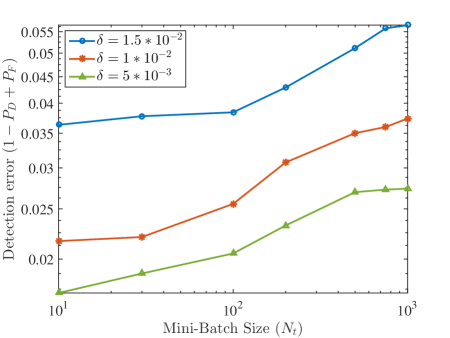
The second experiment varies $N_{t}$, the size of the mini-batches. The batch size $N_{t}$ varies from 10 to 1000. Fig. 6 displays the detection error as a function of $N_{t}$. The three curves correspond to different subspace rotation speed ($\delta$). The detection error increases slightly as $N_{t}$ increase, since reducing $N_{t}$ in general improves the ability of the algorithm to follow the changing subspaces. For all three values of $\delta$, the change in detection error relative to $N_{t}$ is less than 2%.

Figure 6: Detection error as a function of mini-batch size $N_{t}$. The three curves correspond to different subspace changing speeds ($\delta$). The detection error increases as $N_{t}$ increases. For all three $\delta$ values, the change in detection error relative to $N_{t}$ is less than 2%.

5 Synthetic data experiments

This section compares the Online Thinning approach based on tracking a dynamic low-rank GMM with (a) a classical full-rank static GMM and (b) an online GMM estimation algorithm. Neither of these comparators has the low-rank structure exploited by the Online Thinning algorithm. The synthetic data is generated according to the same model as in Section 4.

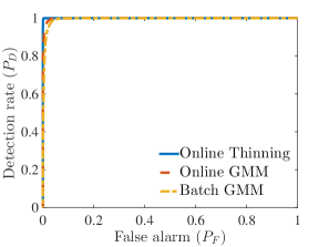
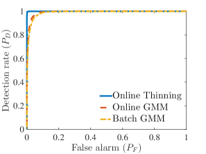
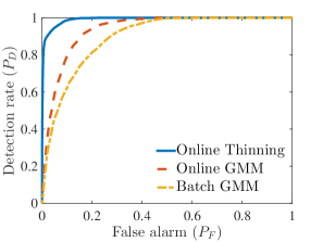
The experiment streams in four thousand observations in total. For Online Thinning and the classical online GMM, an initial model is estimated using the first one thousand samples, and the models are then updated in an online fashion for the remaining three thousand samples. The anomalousness score is calculated as the negative log-likelihood of each data point according to the estimated model. For the classical static GMM algorithm, we estimate a GMM model on the entire four thousand data points (after all samples come in) at once, and assign an anomalousness score to each sample proportional to the negative log likelihood of the data point coming from the estimated GMM model. Fig. 7 compares the detection accuracy (in ROC curves) of Online Thinning and the two comparator algorithms in two settings, where in 7a, the true subspaces used to generate the data are kept static throughout the experiment, and in 7b and 7c, the true subspaces rotate at a small rate ($5\times 10^{-3}$ and $2\times 10^{-2}$, respectively) at each time step. Each plotted experiment is averaged over thirty random realizations. As seen in the plots, Online Thinning using the dynamic low-rank GMM outperforms the online and static algorithms based on a classical full-rank GMM model in all cases, especially when the subspaces change over time.

The reasons behind the performance gap when the subspaces change over time can be explained by the underlying models of the three algorithms. Both the batch GMM and online GMM algorithms rely on full-rank GMM models, which make the problem ill-posed, and, therefore, estimating the covariance matrices becomes difficult. Furthermore, the batch GMM algorithm relies on a static model, which introduces bias when the environment is dynamic. On the other hand, Online Thinning is based on a dynamic low-rank GMM model, and thus faces a much less ill-posed problem by having a union of subspace assumption (which significantly reduces the number of unknowns in the covariance matrices). At the same time, Online Thinning focuses on the most recent samples by weighing down the past samples, and can thus follow the changes in the subspaces.

(a) Static subspaces

(b) Subspaces changing at rate $5\times 10^{-3}$

(c) Subspaces changing at rate $2\times 10^{-2}$

Figure 7: Comparison between Online Thinning using a dynamic low-rank GMM, a classical online GMM, and a classical static batch GMM assuming true subspace rank (ten) is known. 7a shows the comparison between Online Thinning and GMM when the subspaces are static. 7b and 7c show the comparison between Online Thinning and GMM when the subspaces change at a rate of $5\times 10^{-3}$ and $2\times 10^{-2}$, respectively. Online Thinning outperforms both the online and batch GMM algorithms in all cases, especially when the subspaces change over time.

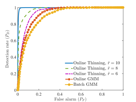
In Fig. 7, the true subspace rank is assumed known. However, the real rank of the subspaces is not always known a priori. To further assess the performance of Online Thinning in such situations, we repeat the above experiment but compute rank-six and rank-eight approximations of the rank-ten subspaces; the results are displayed in Fig. 8. Note that the classical (full-rank) GMM algorithms are not affected by the rank assumption. As seen in the plots, the performance of Online Thinning slightly degrades when the rank of the subspace is given incorrectly to the algorithm. However, Online Thinning still outperforms the classical batch GMM and online GMM algorithms when the subspaces rotates at a rate of $\delta=1\times 10^{-2}$, even when the rank of the subspaces is significantly under-estimated.

Figure 8: Comparison between Online Thinning, online GMM and batch GMM assuming the subspace rank is under-estimated at six and eight for the Online Thinning algorithm. We show the comparison between Online Thinning, online GMM and regular GMM algorithms when the subspaces change at a rate of $1\times 10^{-2}$. Even when the rank is incorrectly estimated at six (correct rank is ten), Online Thinning outperforms both classical batch GMM and online GMM algorithms.

6 Wide-area motion imagery experiments

This experiment compares Online Thinning with the SUN (Saliency Using Natural statistics) algorithm proposed by Zhang et al in [67]. The SUN algorithm is representative of the state-of-the-art saliency detection algorithms [89], provides a general framework for many models, performs as well as or better than previous models, and is computationally efficient [67].

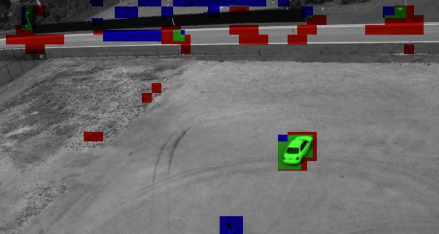
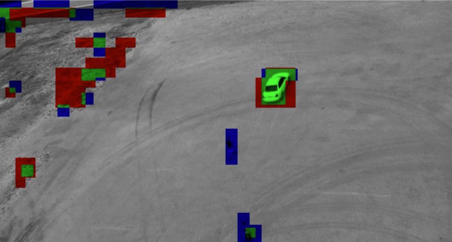
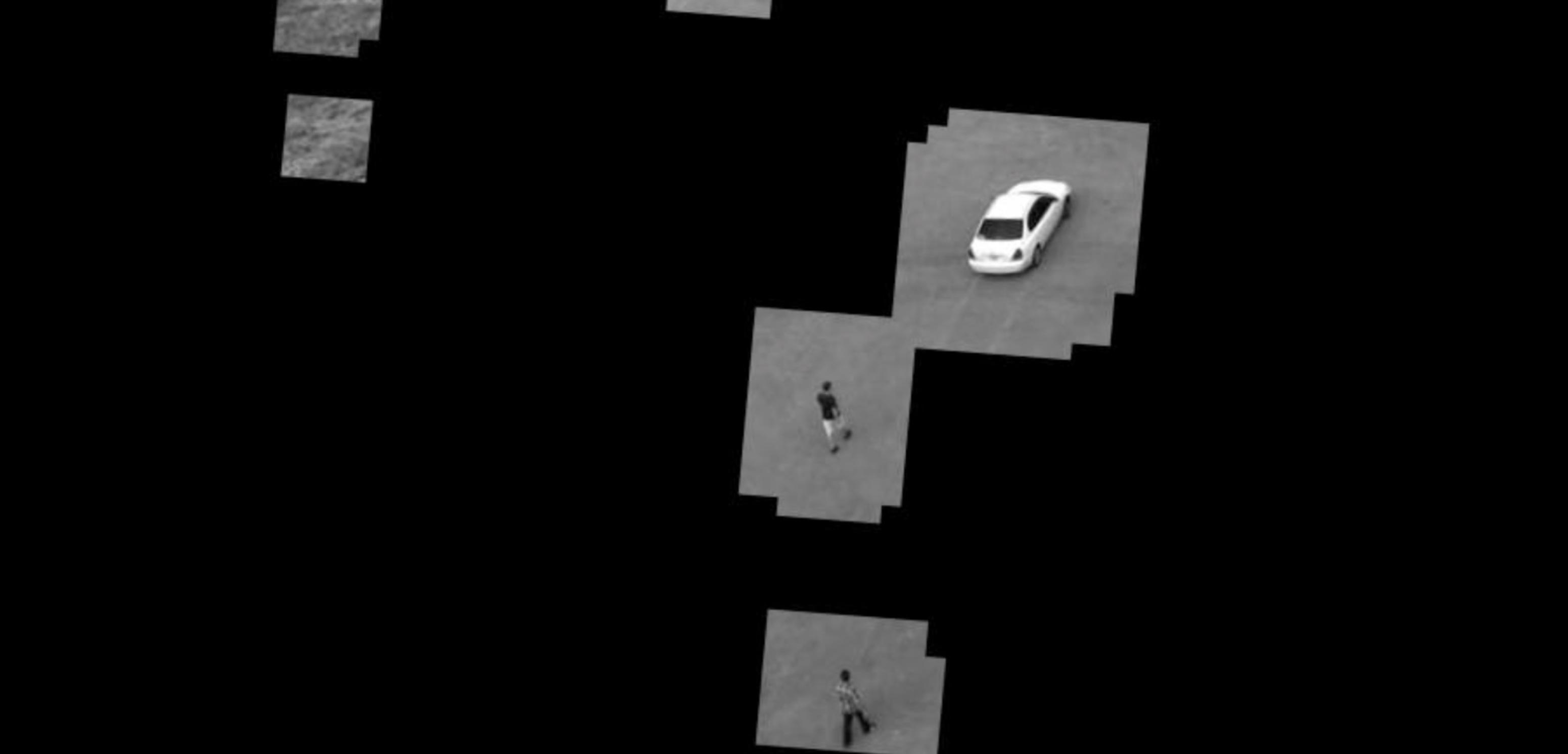
We perform this comparison on a real surveillance video capturing an empty field near a highway. In the video, a car is parked on the lot, and two people can be seen walking in and out of the scene on the field. We use this video because it is clear that the car and the people are most salient in the scene. The original video can be found at https://youtu.be/mX1TtGdGFMU. For the Online Thinning algorithm, we use SIFT (scale-invariant feature transform) features [90] of frame $t$ as our observation $X_{t}$ at time $t$. Specifically, we use the package from [91] to compute the dense SIFT features (i.e., SIFT features computed over a pre-set grid of points on each frame) as features. Each frame of the video is of size $960\times 540$, and the grid is placed so that one SIFT feature is computed for each $25\times 25$ patch. Each frame have roughly eight hundred SIFT feature vectors. The dimension of each SIFT feature vector is 128.

Fig. 9 shows the result of Online Thinning and the SUN algorithms on this surveillance video at frames 50 and 100. Figures 9a and 9b show the original frames, while in 9c and 9d, we flag the top 5% patches with the highest anomalousness or saliency scores by the Online Thinning and SUN algorithms. In the results, green patches are flagged by both methods, blue patches are only flagged by Online Thinning, and red patches are only flagged by SUN. Note that in both frames, the people in the scene are mostly labeled by blue, i.e., they are only flagged by Online Thinning. The Online Thinning outperforms the SUN algorithm by more consistently flagging small rare patches such as the people; this is in part due to the adaptivity of Online Thinning to dynamic environments. The result video can be found at https://www.youtube.com/watch?v=DyLJThawgi0.

(a) Original, frame 50

(b) Original, frame 100

(c) 5% most salient patches, frame 50

(d) 5% most salient patches, frame 100

Figure 9: Data thinning result using Online Thinning and SUN algorithms on the surveillance video at frames 50 and 100. The first row shows the original video, and the second row shows the data thinning results. In the results, green patches are flagged by both methods, blue patches are only flagged by Online Thinning, and red patches are only flagged by SUN. Online Thinning outperforms the SUN algorithm by consistently flagging the people, which are sometimes missed by the SUN algorithm.

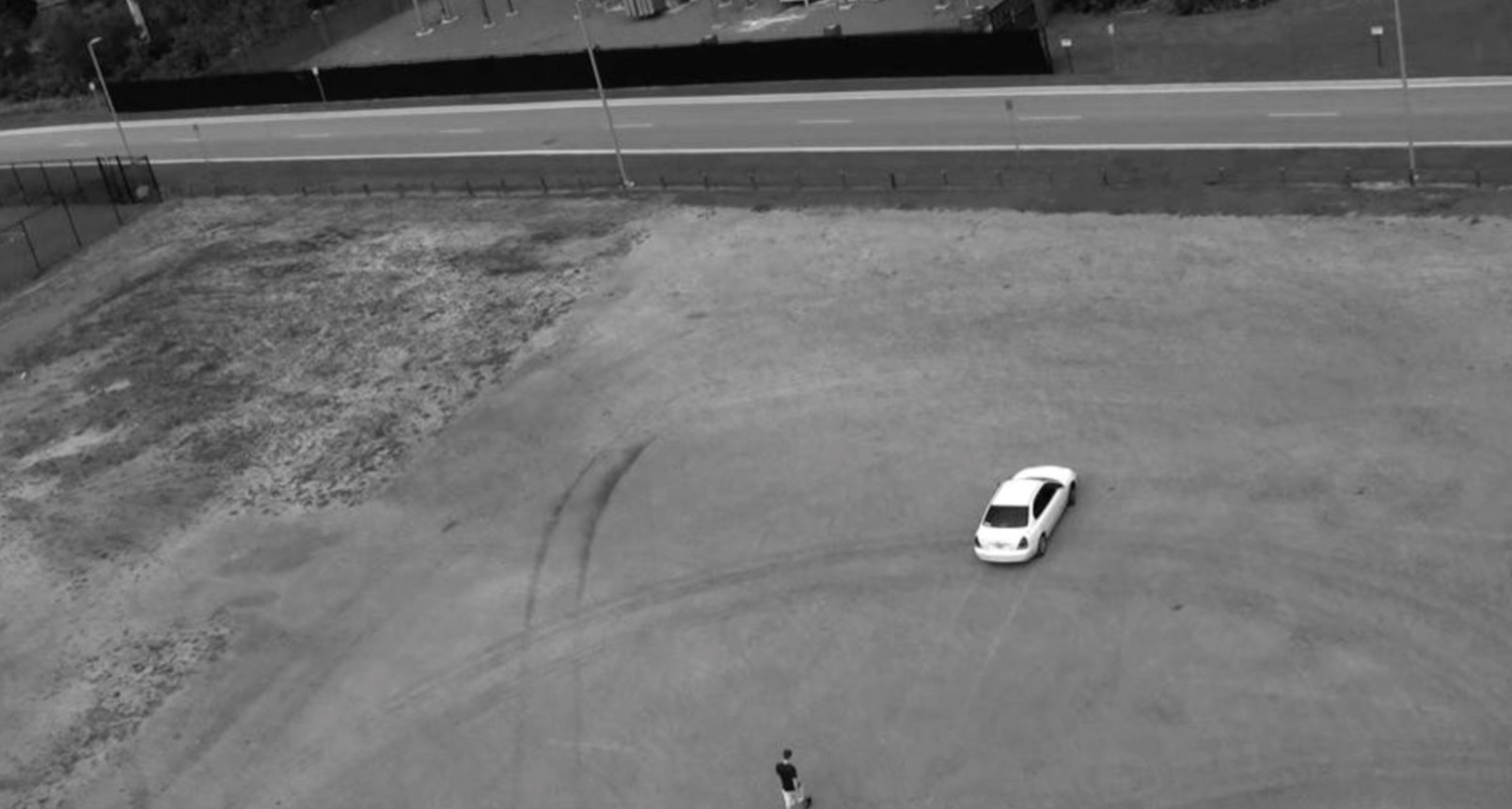
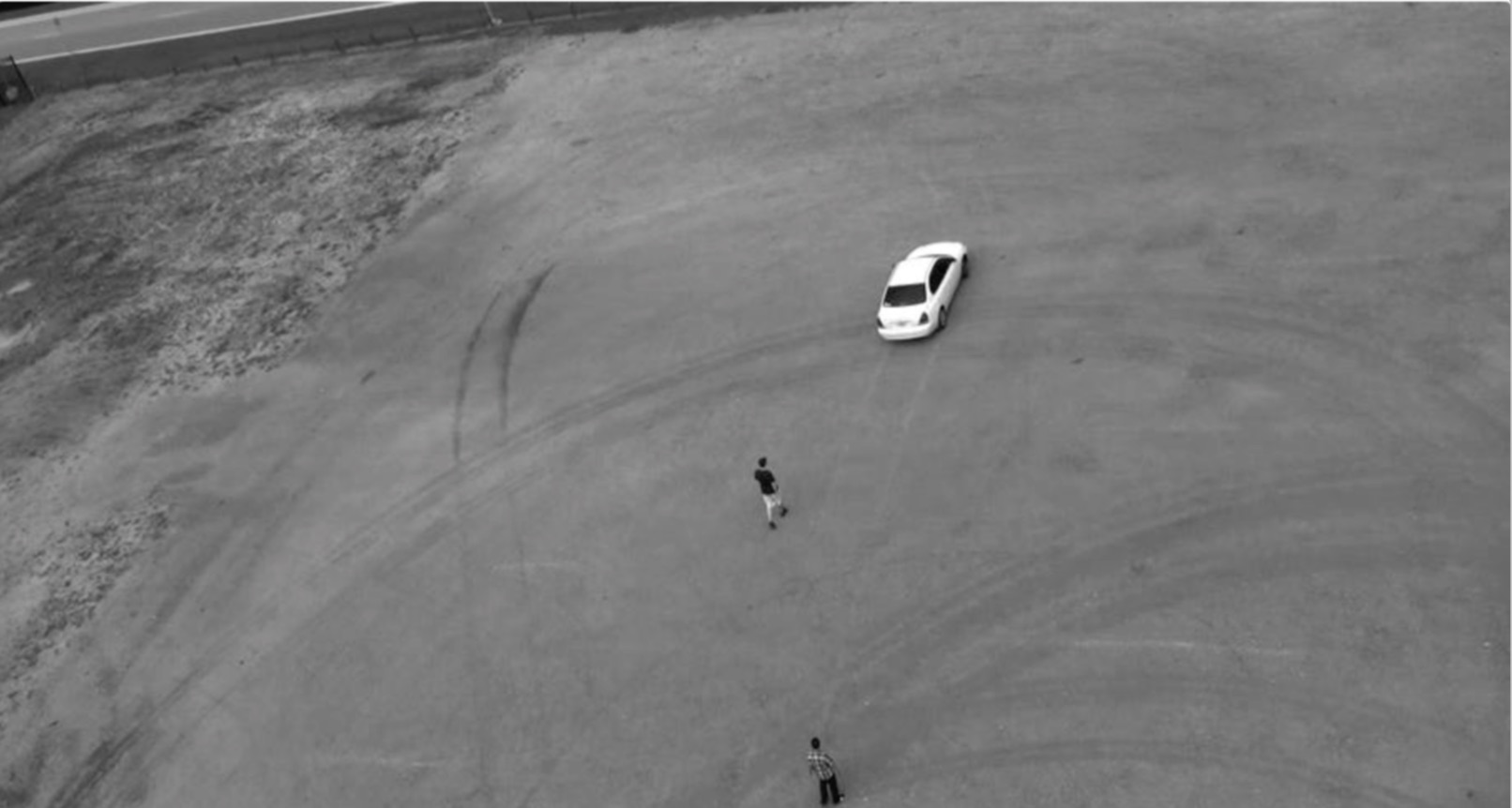
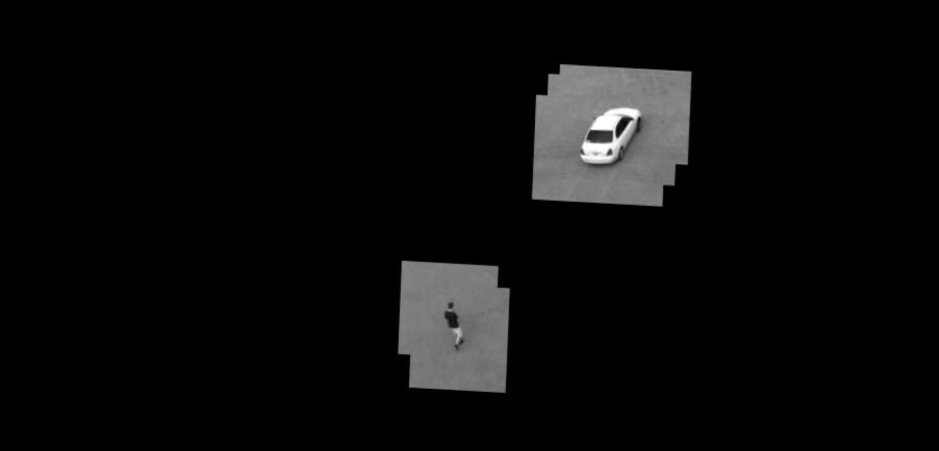
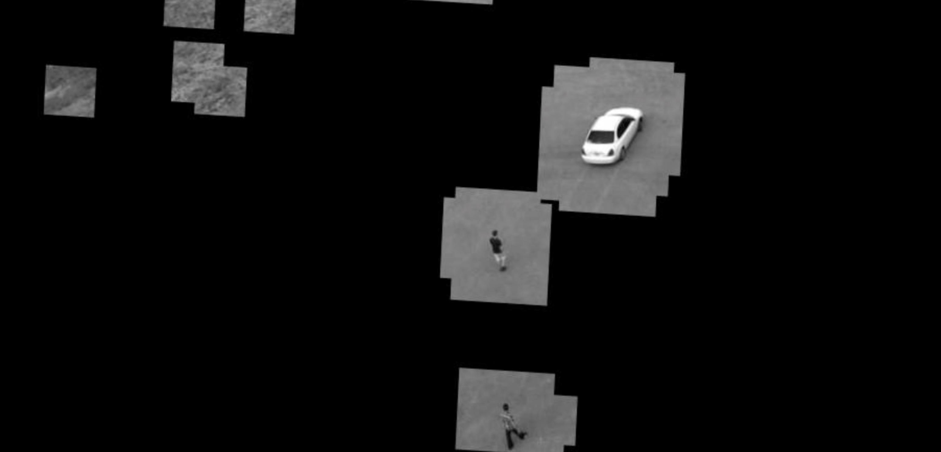
Motion imagery taken from a moving camera (e.g., video taken from an unmanned arial vehicle) is often jittery due to mechanical vibrations in the camera platform. Such jittering often poses difficulty to the data thinning task. The magnitude of the vibrations precludes standard video stabilization techniques used, for instance, for handheld video cameras. This experiment demonstrates that the proposed method can robustly flag salient objects from a jittery video; the flagged patches can then be processed off-line (as discussed in the introduction), and software video-stabilization methods can be applied to these frames alone to co-register them.

Specifically, to demonstrate the effect of jittering, we artificially add random rotations and small shifting to each of the frames before processing. The jittered video can be found at https://youtu.be/oKzIOryxR0s. Then, we flag and extract patches with high anomalousness scores using the proposed Online Thinning algorithm. Finally, we use a feature-matching-based approach on only the flagged patches to generate a stabilized, thinned video [92, 93]. Fig. 10 shows the original jittered video frames (left column) and corresponding stabilized detection results (right column). Note that despite the rotation and shifting of the original frames, the stabilized result is consistently showing the car and the people without significant shifting or shaking. The result video can be found at https://youtu.be/DyLJThawgi0.

(a) Jittering video frame 60

(b) Stabilized detection frame 60

(c) Jittering video frame 61

(d) Stabilized detection frame 61

(e) Jittering video frame 120

(f) Stabilized detection frame 120

(g) Jittering video frame 121

(h) Stabilized detection frame 121

Figure 10: The original, jittered video frames (left columns) and corresponding thinning results after stabilization (right columns). The thinning result consistently shows the car and the people without significant shifting or shaking, even though the stabilization was performed using only the flagged patches.

Under different situations, the meaning of “anomalousness” and “saliency” can also be different. For example, a moving car on a busy street during daytime may be seen as normal, while the same car should be considered anomalous or salient if it appears in some vacant lot when no other cars are around. Conventional non-adaptive saliency detection algorithms often lack the flexibility of changing the definition of saliency over time, while Online Thinning, as an online algorithm, has the ability to learn the environment over time and adapt to new needs.

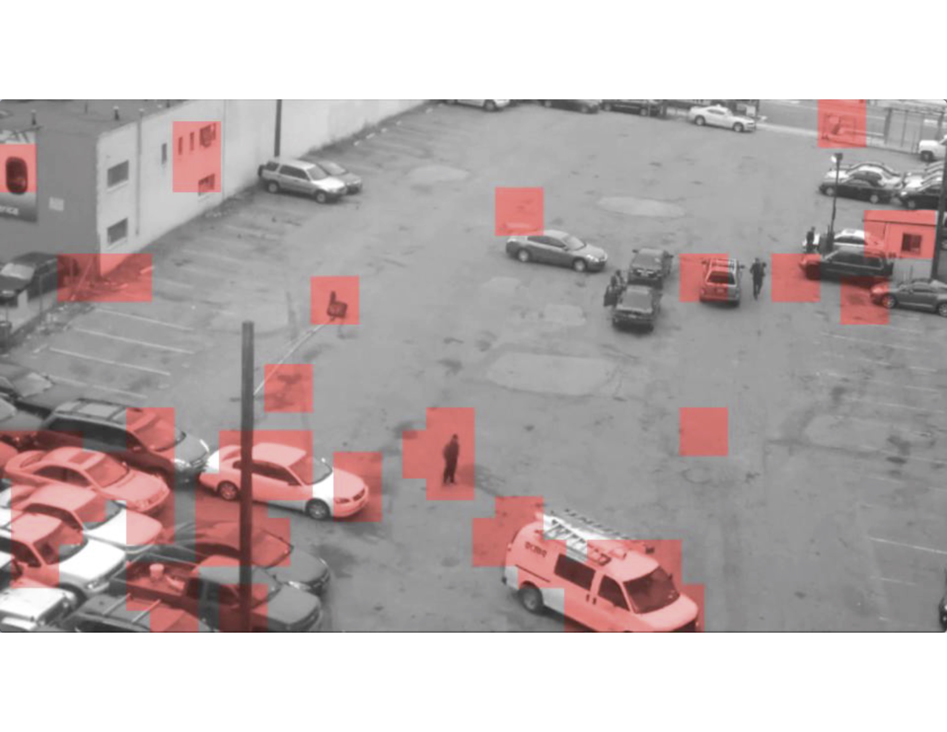
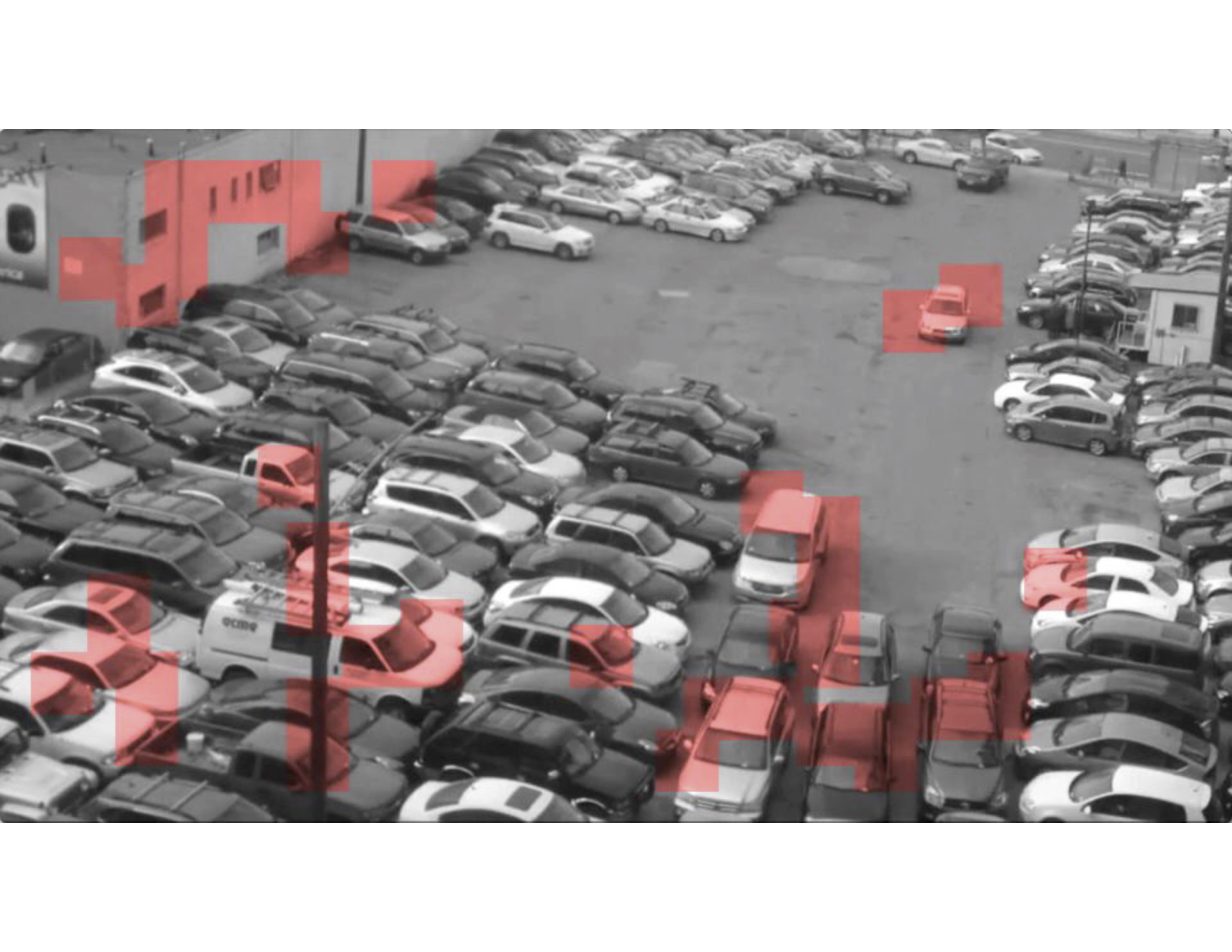
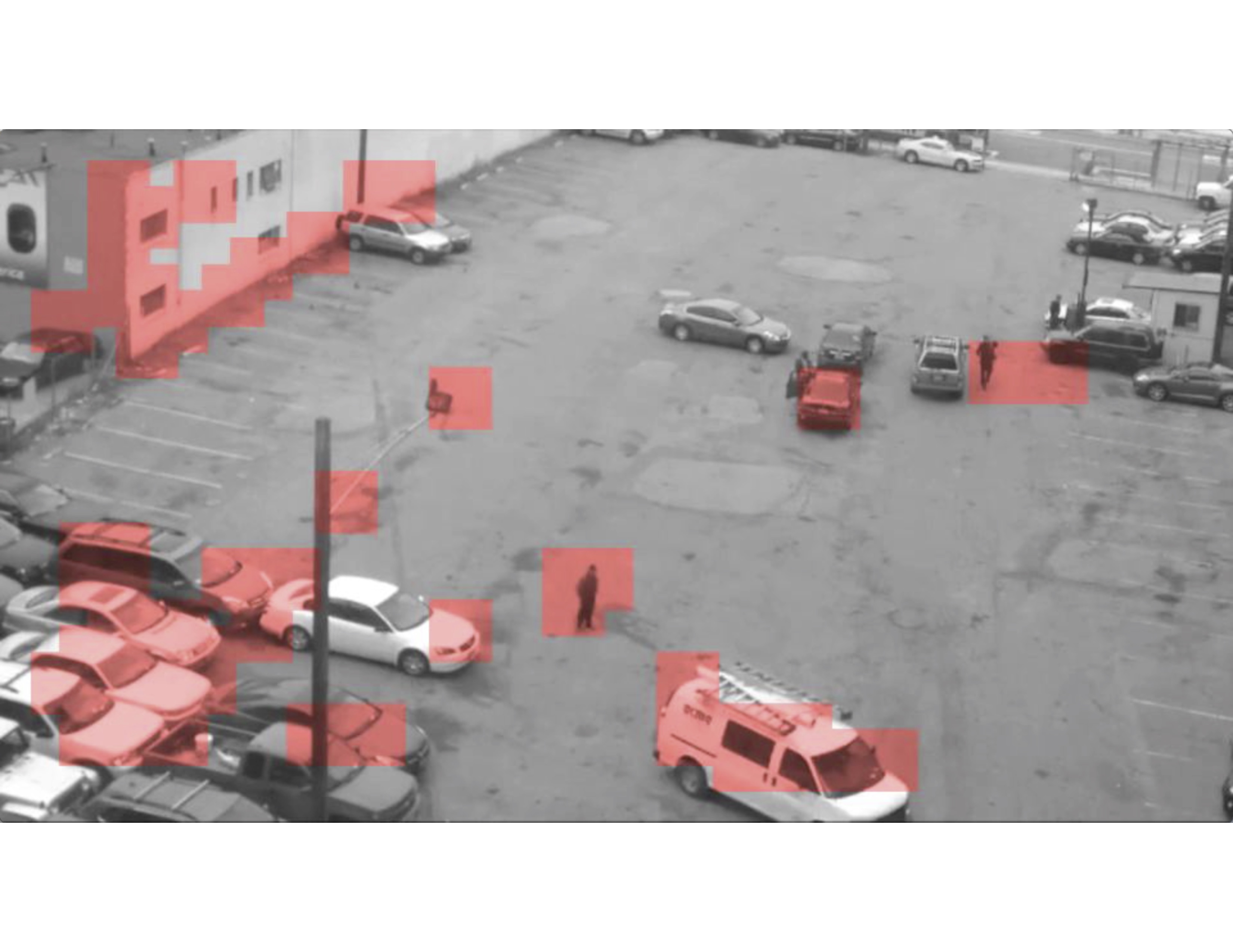
A third experiment compares Online Thinning with the classical batch and online GMM algorithm with a real-life parking lot surveillance video data. The video is a time-lapse of a parking lot where cars arrive and gradually fill up the entire lot. For Online Thinning and the classical online GMM, an initial model is estimated using the first frame, and the models are then updated frame by frame. The anomalousness score is calculated as the negative log-likelihood of each data point according to the estimated model. For the classical static GMM algorithm, we estimate a GMM model on the first twenty frames, and assign an anomalousness score to each data point proportional to the negative log likelihood of the data point coming from the estimated GMM model. The batch GMM is trained only with the patches from the first twenty frames to simulate a setting in which a probability model is learned in one set of environmental conditions and does not adapt to a changing environment.

For all three algorithms, dense SIFT features from each frame $t$ are used as the observation $X_{t}$. Each frame of the video is of size $960\times 540$, and the grid is placed so that one SIFT feature is computed for each $25\times 25$ patch. Each frame have roughly eight hundred SIFT feature vectors. The dimension of each SIFT feature vector is 128.

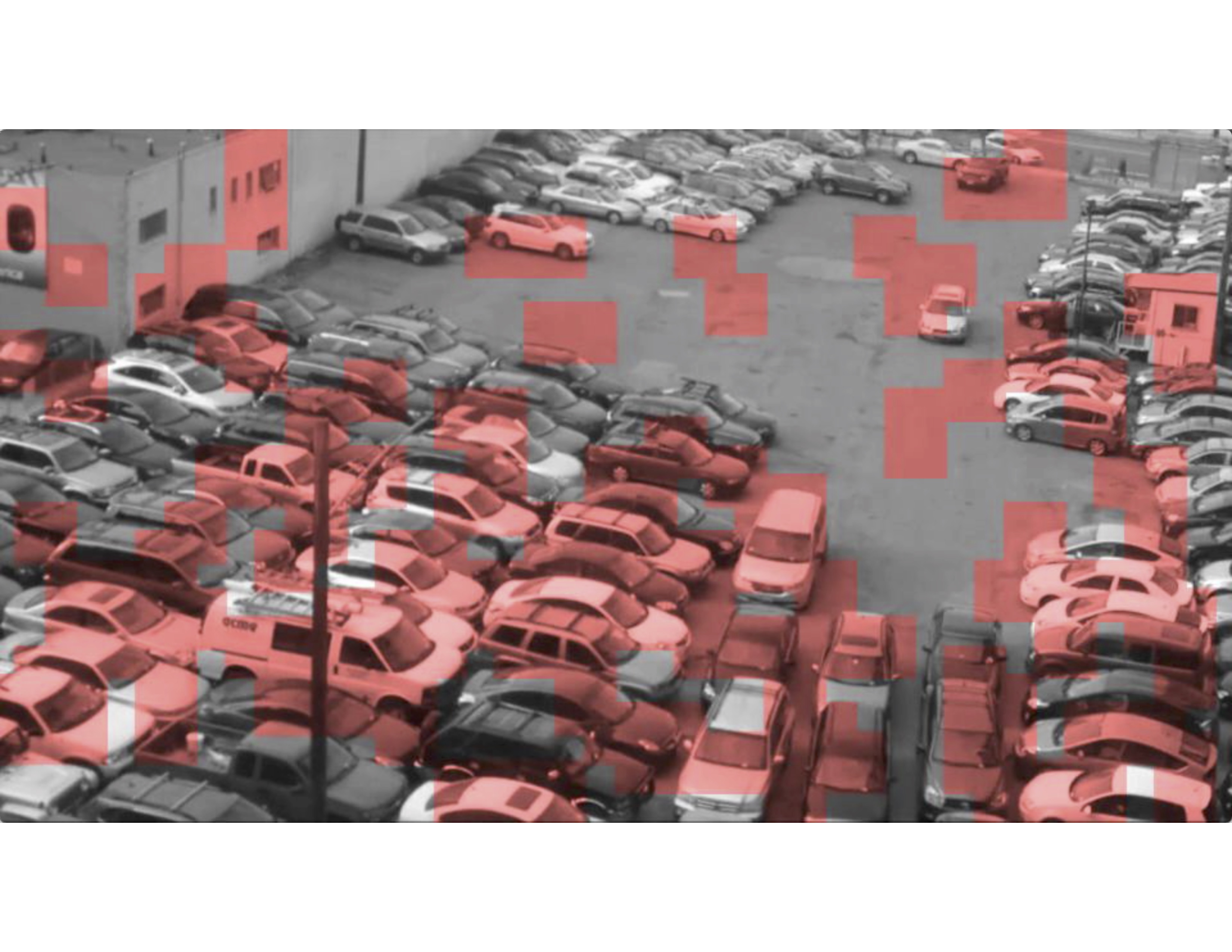
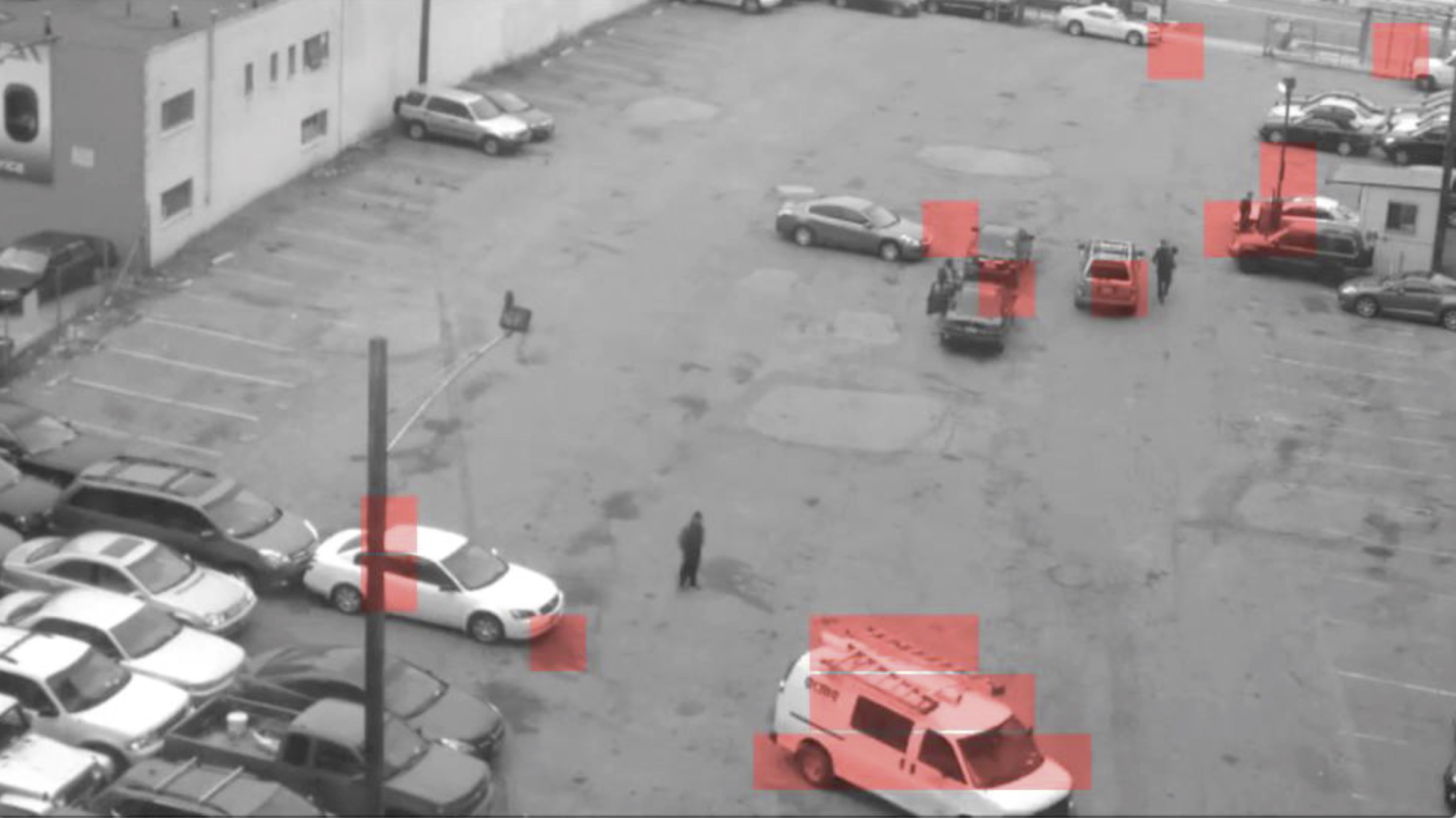
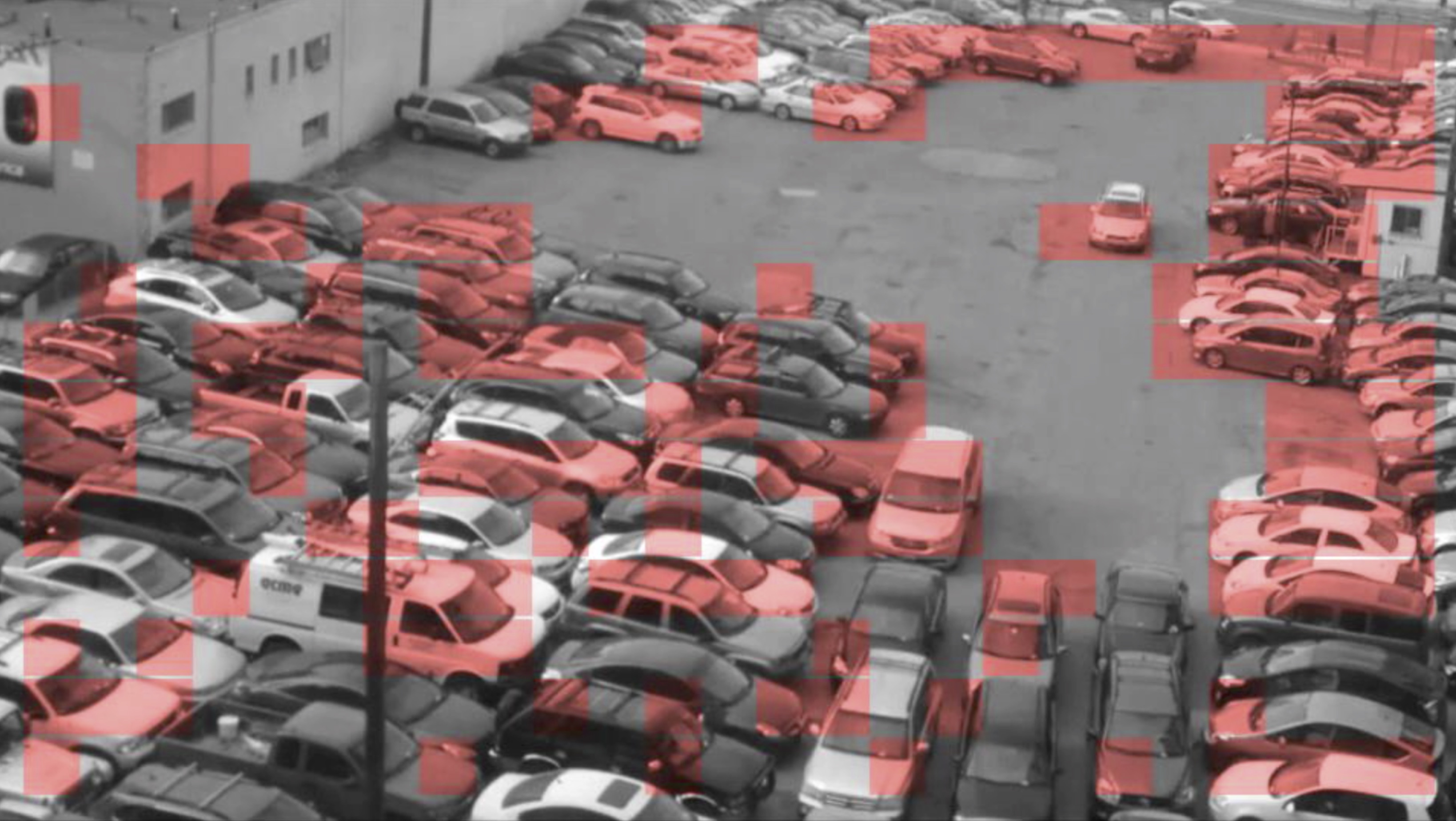
Fig. 11 shows the result of Online Thinning (Alg. 4) and both classical batch and online GMM algorithms on the surveillance video at frames 21 and 232. Red-colored patches are flagged as having high anomalousness scores. Figures 11a,  11c and 11e show the result on frame 21, where the lot is still relatively empty, and all three algorithms flagged similar items in the scene (incoming car, people in the lot). Figures 11b, 11d and 11f show the result on frame 232, when the lot is about half full. At frame 232, the Online Thinning algorithm has learned that cars are common objects in the video, and has thus adapted to assigning lower anomalousness scores to most cars. Instead, the Online Thinning algorithm assigns higher anomalousness scores to relatively uncommon objects like black pole, building windows, and cars parked differently from others. The batch GMM algorithm does not adapt to the video, and assigns most cars with high anomalousness scores. The online GMM algorithm flags fewer patches than the batch GMM algorithm when the parking lot is filled up. However, online GMM still flags significantly more cars than the Online Thinning algorithm. Note that in the video, the parking lot is filled up gradually, and most of the cars in the parking lot at frame 232 has shown up in the scene for a long time. However, at frame 232, the Online GMM algorithm still flags a significant amount of cars in the parking lot, while the Online Thinning algorithm has stopped flagging cars that have been in the scene for a long time. This suggests that the online GMM algorithm adapts to the environment at a slower rate than the Online Thinning algorithm.

(a) Online Thinning, frame 21

(b) Online Thinning, frame 232

(c) Batch GMM, frame 21

(d) Batch GMM, frame 232

(e) Online GMM, frame 21

(f) Online GMM, frame 232

Figure 11: Result of Online Thinning and classical batch and online GMM algorithms on the surveillance video at frames 21 and 232. Red-colored patches are flagged as salient according to the different probability models. 11a, 11c, and 11e show the result on frame 21, where the lot is still relatively empty, and all three algorithms flag similar items in the scene (incoming car, people in the lot). 11b, 11d, and 11f show the result on frame 232, when the lot is about half full. The Online Thinning algorithm has learned that cars are common objects in the video, and has thus adapted to assigning lower anomalousness scores to most cars. The batch GMM algorithm does not adapt to the video, and assigns most cars with high anomalousness scores. The online GMM algorithm flags less cars with high anomalousness scores than batch GMM algorithm, but still flags more cars than the Online Learning algorithm. This suggests the online GMM algorithm adapts to the environment slower than the Online Learning algorithm.

7 Enron email experiments

Data thinning can also be applied to text documents to find anomalous texts and topics. The development of latent Dirichlet allocation (LDA) [94] for text document topic modeling and other methods have allowed us to analyze the topics of a collection of documents. The Enron data is a collection of about fifty thousand emails within the Enron corporation between the year 1998 and 2002. The dataset has been explored in the context of social network analysis [95] and event detection [96, 97, 98]. In [97, 98], the authors used the email addresses and time stamps and successfully predicted major events in the company by finding days during which email correspondence shows abnormal patterns. In our work, we also try to detect significant events in the company’s history by using the Enron database. However, we approach the problem by using the count of “topic words” found in the emails, instead of the contact information which does not reflect the content of the emails.

The challenge here is that the count data cannot be modeled as Gaussian, and pre-processing is needed before applying the method. We see each of the word-count of topic words in the email as an independent Poisson realization of some underlying rate. By using the Anscombe transformation [99], we can approximate the normalized data as arising from a Gaussian mixture model, and thus apply the Online Thinning Algorithm 4.

This experiment applies the Online Thinning algorithm to the Enron email dataset for event detection. To process the Enron emails, we first generate a five-hundred-word topic list using LDA [100], where the list includes fifty topics, and each topic has ten associated keywords. For each email, the number of times each keyword appears is counted and recorded in a fifty-dimensional vector $y_{t}\in\mathbb{N}^{50}$ where each entry $[y_{t}]_{i}$ corresponds to how many times the keywords in topic $i$ appears in this email. Here $[\cdot]_{i}$ indicates the $i^{\mbox{th}}$ element of a vector. The feature vectors are then normalized using the Anscombe transform [101] by setting $[x_{t}]_{i}=2\sqrt{[y_{t}]_{i}+\frac{3}{8}};$ note that $[x_{t}]_{i}$ is asymptotically normal with mean $2\sqrt{[y_{t}]_{i}+\frac{3}{8}}+\frac{1}{4\sqrt{[y_{t}]_{i}}}$ and unit variance. Online Thinning is then applied to the transformed data data (the $x_{t}$’s), and we flag emails by thresholding the anomalousness score assigned by the Online Thinning algorithm.

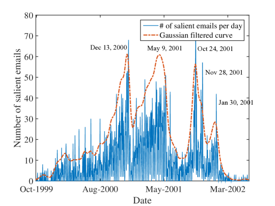
Fig. 12 shows the number of selected emails versus time (date). The major peaks in the plot correspond to the following time and events:

1. December 13, 2000: Enron announces that president and chief operating officer Jeffrey Skilling will take over as chief executive in February. [102]

2. May 9, 2001: “California utility says prices of gas were inflated” by Enron collaborator, and blackouts affect 167,00 Enron customers. [103, 104]

3. October 24, 2001: Enron ousts its chief financial officer Andrew S. Fastow, and the shares of Enron fell to the lowest price since early 1995 [105].

4. November 28, 2001: Enron shares plunge below $1. [106]

5. January 30, 2001: Stephen Cooper takes over as Enron CEO, and Enron Metals is sold to a unit of Sempra Energy. [107, 108]

As seen, the flagged dates cluster around the time when significant events happen in the Enron company.

Figure 12: number of selected emails versus time (date). The large peaks in the plot all correspond to major events in the history of the company. The red curve is smoothed using a Gaussian filter.

8 Conclusion

This paper proposed an online data thinning method for high-dimensional data with changing environment. At the heart of the proposed algorithm is a union of subspaces tracking algorithm, which allows for fast and accurate data thinning in a variety of applications with both subsampled data and mini-batch updates.

The core idea of the proposed approach is to track a Gaussian mixture model whose covariance matrices each are dominated by a low-rank component. Under this model, most observations are concentrated in a union of subspaces, a model growing in popularity in image, video, and text analysis because of its flexibility and robustness to over-fittings. Unlike traditional GMMs, the low-rank structure proposed here mitigates the curse of dimensionality and facilitates efficient tracking in dynamic environments. Furthermore, by leveraging the recent advances in subspace tracking and subspace clustering techniques, the proposed method is able to accurately estimate the mixture density without adding a significant computational burden. Another important feature of the proposed method is the ability to track an arbitrary number of mixture components. The adoption of a tree-like hierarchical structure for the union of subspaces model allows the method to adaptively choose the number of subspaces needed at each time stamp, and thus greatly improves the flexibility of the method and accuracy when tracking highly dynamic densities.

References

- [1] W. Pincus and D. Priest. NSA intercepts on eve of 9/11 sent a warning: Messages translated after attacks, June 20, 2002. The Washington Post, Page A01.
- [2] W. Clavin. Managing the deluge of ‘big data’ from space, 2013. http://www.jpl.nasa.gov/news/news.php?release=2013-299.
- [3] J. Marlow. What to do with 1,000,000,000,000,000,000 bytes of astronomical data per day, 2012. Wired, http://www.wired.com/2012/04/what-to-do-with-1000000000000000000-bytes-of-astronomical-data-per-day/.
- [4] LSST Team. LSST: A new telescope concept. http://www.lsst.org/lsst/public/tour_software, retrieved June 7, 2014.
- [5] Z. Ivezic and et al. (108 additional authors not shown). LSST: from science drivers to reference design and anticipated data products. http://arxiv.org/abs/0805.2366arXiv:0805.2366, 2008.
- [6] E. Dumbill. What is big data? An introduction to the big data landscape, 2012. http://strata.oreilly.com/2012/01/what-is-big-data.html.
- [7] M. Raginsky, R. Willett, C. Horn, J. Silva, and R. Marcia. Sequential anomaly detection in the presence of noise and limited feedback. IEEE Trans. Info. Theory, 58(8):5544 – 5562, Aug. 2012.
- [8] C. Horn and R. Willett. Online anomaly detection with expert system feedback in social networks. In Proc. International Conference on Acoustics, Speech, and Signal Processing, 2011.
- [9] R. Bellman. Adaptive control processes: a guided tour, volume 4. Princeton University Press, Princeton, NJ, 1961.
- [10] T. Hastie, R. Tibshirani, and J. Friedman. The Elements of Statistical Learning: Data Mining, Inference, and Prediction. Springer-Verlag New York, 2009.
- [11] Doug Bezier. BAE to develop surveillance system. The Washington Post, 2007. Retrieved 3-20-2012.
- [12] D. Hambling. Special forces gigapixel flying spy sees all, 2009. http://www.wired.com/dangerroom/2009/02/gigapixel-flyin/.
- [13] D. J. Brady, M. E. Gehm, R. A. Stack, D. L. Marks, D. S. Kittle, D. R. Golish, E. M. Vera, and S. D. Feller. Multiscale gigapixel photography. Nature, 486:386–389, 2012.
- [14] K. Bourzac. Gigapixel camera catches the smallest details. Nature News, 2012.
- [15] L. Greenemeier. Draw the curtains: Gigapixel cameras create highly revealing snapshots, 2011. http://www.scientificamerican.com/article.cfm?id=gigapixel-camera-revealed.
- [16] L. Itti, C. Koch, and E. Niebur. A model of saliency-based visual attention for rapid scene analysis. IEEE Transactions on Pattern Analysis & Machine Intelligence, 20(11):1254–1259, 1998.
- [17] X. Hou and L. Zhang. Saliency detection: A spectral residual approach. In Computer Vision and Pattern Recognition, 2007. CVPR’07. IEEE Conference on, pages 1–8. IEEE, 2007.
- [18] J. Harel, C. Koch, and P. Perona. Graph-based visual saliency. In Advances in neural information processing systems, pages 545–552, 2006.
- [19] N. Rao, J. Harrison, T. Karrels, R. Nowak, and T. T. Rogers. Using machines to improve human saliency detection. In Signals, Systems and Computers (ASILOMAR), 2010 Conference Record of the Forty Fourth Asilomar Conference on, pages 80–84. IEEE, 2010.
- [20] S. Ertürk. Real-time digital image stabilization using kalman filters. Real-Time Imaging, 8(4):317–328, 2002.
- [21] M. Hansen, P. Anandan, K. Dana, G. Van der Wal, and P. Burt. Real-time scene stabilization and mosaic construction. In Applications of Computer Vision, 1994., Proceedings of the Second IEEE Workshop on, pages 54–62. IEEE, 1994.
- [22] K. Ratakonda. Real-time digital video stabilization for multi-media applications. In Circuits and Systems, 1998. ISCAS’98. Proceedings of the 1998 IEEE International Symposium on, volume 4, pages 69–72. IEEE, 1998.
- [23] H.-C. Chang, S.-H. Lai, and K.-R. Lu. A robust real-time video stabilization algorithm. Journal of Visual Communication and Image Representation, 17(3):659–673, 2006.
- [24] S. Battiato, A. R. Bruna, and G. Puglisi. A robust block-based image/video registration approach for mobile imaging devices. Multimedia, IEEE Transactions on, 12(7):622–635, 2010.
- [25] A. Samé, C. Ambroise, and G. Govaert. An online classification em algorithm based on the mixture model. Statistics and Computing, 17(3):209–218, 2007.
- [26] L. Balzano, R. Nowak, and B. Recht. Online identification and tracking of subspaces from highly incomplete information. In Proc. Allerton Conf. on Comm., Control and Comp., pages 704 – 711, Sept. 2010.
- [27] Y. Chi, Y. C. Eldar, and R. Calderbank. Petrels: Parallel estimation and tracking of subspace by recursive least squares from partial observations. submitted to IEEE Trans. Sig. Proc., arXived., July 2012.
- [28] Y. Chi, Y. C. Eldar, and R. Calderbank. PETRELS: Subspace estimation and tracking from partial observations. In IEEE Int. Conf. on Acoustics, Speech and Sig. Proc. (ICASSP), 2012.
- [29] H. Mansour and X. Jiang. A robust online subspace estimation and tracking algorithm. In IEEE International Conference on Acoustics, Speech and Signal Processing (ICASSP), April 2015.
- [30] C. C. Aggarwal and P. S. Yu. Finding generalized projected clusters in high dimensional spaces, volume 29. ACM, 2000.
- [31] P. S. Bradley and O. L. Mangasarian. k-plane clustering. Journal of Global Optimization, 16(1):23–32, 2000.
- [32] C. Böhm, K. Kailing, P. Kröger, and A. Zimek. Computing clusters of correlation connected objects. In Proceedings of the 2004 ACM SIGMOD international conference on Management of data, pages 455–466. ACM, 2004.
- [33] E. Achtert, C. Böhm, P. Kröger, and A. Zimek. Mining hierarchies of correlation clusters. In Scientific and Statistical Database Management, 2006. 18th International Conference on, pages 119–128. IEEE, 2006.
- [34] E. Achtert, C. Böhm, H.-P. Kriegel, P. Kröger, and A. Zimek. Robust, complete, and efficient correlation clustering. In SDM, pages 413–418. SIAM, 2007.
- [35] E. Achtert, C. Böhm, H.-P. Kriegel, P. Kröger, and A. Zimek. On exploring complex relationships of correlation clusters. In Scientific and Statistical Database Management, 2007. SSBDM’07. 19th International Conference on, pages 7–7. IEEE, 2007.
- [36] F. Y. Edgeworth. Xli. on discordant observations. The London, Edinburgh, and Dublin Philosophical Magazine and Journal of Science, 23(143):364–375, 1887.
- [37] V. Chandola, A. Banerjee, and V. Kumar. Anomaly detection: A survey. ACM computing surveys (CSUR), 41(3):15, 2009.
- [38] C. De Stefano, C. Sansone, and M. Vento. To reject or not to reject: that is the question-an answer in case of neural classifiers. Systems, Man, and Cybernetics, Part C: Applications and Reviews, IEEE Transactions on, 30(1):84–94, 2000.
- [39] D. Barbara, N. Wu, and S. Jajodia. Detecting novel network intrusions using bayes estimators. In SDM, pages 1–17. SIAM, 2001.
- [40] B. Schölkopf, J. C. Platt, J. Shawe-Taylor, A. J. Smola, and R. C. Williamson. Estimating the support of a high-dimensional distribution. Neural computation, 13(7):1443–1471, 2001.
- [41] V. Roth. Outlier detection with one-class kernel fisher discriminants. In Advances in Neural Information Processing Systems, pages 1169–1176, 2004.
- [42] V. Roth. Kernel fisher discriminants for outlier detection. Neural computation, 18(4):942–960, 2006.
- [43] J. Zhang and H. Wang. Detecting outlying subspaces for high-dimensional data: the new task, algorithms, and performance. Knowledge and information systems, 10(3):333–355, 2006.
- [44] M. E. Otey, A. Ghoting, and S. Parthasarathy. Fast distributed outlier detection in mixed-attribute data sets. Data Mining and Knowledge Discovery, 12(2-3):203–228, 2006.
- [45] A. Ghoting, S. Parthasarathy, and M. E. Otey. Fast mining of distance-based outliers in high-dimensional datasets. Data Mining and Knowledge Discovery, 16(3):349–364, 2008.
- [46] Y. Tao, X. Xiao, and S. Zhou. Mining distance-based outliers from large databases in any metric space. In Proceedings of the 12th ACM SIGKDD international conference on Knowledge discovery and data mining, pages 394–403. ACM, 2006.
- [47] M. Wu and C. Jermaine. Outlier detection by sampling with accuracy guarantees. In Proceedings of the 12th ACM SIGKDD international conference on Knowledge discovery and data mining, pages 767–772. ACM, 2006.
- [48] L. Ertöz, M. Steinbach, and V. Kumar. Finding topics in collections of documents: A shared nearest neighbor approach. Springer, 2004.
- [49] D. Yu, G. Sheikholeslami, and A. Zhang. Findout: finding outliers in very large datasets. Knowledge and Information Systems, 4(4):387–412, 2002.
- [50] S. Budalakoti, A. Srivastava, R. Akella, and E. Turkov. Anomaly detection in large sets of high-dimensional symbol sequences. NASA Ames Research Center, Tech. Rep. NASA TM-2006-214553, 2006.
- [51] A. Pires and C. Santos-Pereira. Using clustering and robust estimators to detect outliers in multivariate data. In Proceedings of the International Conference on Robust Statistics, 2005.
- [52] H. E. Solberg and A. Lahti. Detection of outliers in reference distributions: performance of horn?s algorithm. Clinical chemistry, 51(12):2326–2332, 2005.
- [53] C. C. Aggarwal and P. S. Yu. Outlier detection with uncertain data. In SDM, volume 483, page 493. SIAM, 2008.
- [54] D. Chen, X. Shao, B. Hu, and Q. Su. Simultaneous wavelength selection and outlier detection in multivariate regression of near-infrared spectra. Analytical Sciences, 21(2):161–166, 2005.
- [55] D. Agarwal. Detecting anomalies in cross-classified streams: a bayesian approach. Knowledge and information systems, 11(1):29–44, 2007.
- [56] Z. He, S. Deng, and X. Xu. An optimization model for outlier detection in categorical data. In Advances in Intelligent Computing, pages 400–409. Springer, 2005.
- [57] S. Ando. Clustering needles in a haystack: An information theoretic analysis of minority and outlier detection. In Data Mining, 2007. ICDM 2007. Seventh IEEE International Conference on, pages 13–22. IEEE, 2007.
- [58] E. Keogh, S. Lonardi, and C. A. Ratanamahatana. Towards parameter-free data mining. In Proceedings of the tenth ACM SIGKDD international conference on Knowledge discovery and data mining, pages 206–215. ACM, 2004.
- [59] A. Agovic, A. Banerjee, A. R. Ganguly, and V. Protopopescu. Anomaly detection in transportation corridors using manifold embedding. Knowledge Discovery from Sensor Data, pages 81–105, 2008.
- [60] H. Dutta, C. Giannella, K. D. Borne, and H. Kargupta. Distributed top-k outlier detection from astronomy catalogs using the demac system. In SDM, pages 473–478. SIAM, 2007.
- [61] T. Ide and H. Kashima. Eigenspace-based anomaly detection in computer systems. In Proceedings of the tenth ACM SIGKDD international conference on Knowledge discovery and data mining, pages 440–449. ACM, 2004.
- [62] M.-L. Shyu, S.-C. Chen, K. Sarinnapakorn, and L. Chang. A novel anomaly detection scheme based on principal component classifier. Technical report, DTIC Document, 2003.
- [63] M. M. Breunig, H.-P. Kriegel, R. T. Ng, and J. Sander. Lof: identifying density-based local outliers. In ACM sigmod record, volume 29, pages 93–104. ACM, 2000.
- [64] H.-P. Kriegel, A. Zimek, et al. Angle-based outlier detection in high-dimensional data. In Proceedings of the 14th ACM SIGKDD international conference on Knowledge discovery and data mining, pages 444–452. ACM, 2008.
- [65] T. Ahmed. Online anomaly detection using kde. In Global Telecommunications Conference, 2009. GLOBECOM 2009. IEEE, pages 1–8. IEEE, 2009.
- [66] N. Bruce and J. Tsotsos. Saliency based on information maximization. In Advances in neural information processing systems, pages 155–162, 2005.
- [67] L. Zhang, M. H. Tong, T. K. Marks, H. Shan, and G. W. Cottrell. SUN: A Bayesian framework for saliency using natural statistics. Journal of vision, 8(7):32, 2008.
- [68] K. Beyer, J. Goldstein, R. Ramakrishnan, and U. Shaft. When is “nearest neighbor” meaningful? In Database Theory?ICDT’99, pages 217–235. Springer, 1999.
- [69] E. Elhamifar and R. Vidal. Sparse subspace clustering. In Computer Vision and Pattern Recognition, 2009. CVPR 2009. IEEE Conference on, pages 2790–2797. IEEE, 2009.
- [70] E. Elhamifar and R. Vidal. Sparse subspace clustering: Algorithm, theory, and applications. Pattern Analysis and Machine Intelligence, IEEE Transactions on, 35(11):2765–2781, 2013.
- [71] Y.-X. Wang and H. Xu. Noisy sparse subspace clustering. Journal of Machine Learning Research, 17(12):1–41, 2016.
- [72] R. Vidal. A tutorial on subspace clustering. IEEE Signal Processing Magazine, 28(2):52–68, 2010.
- [73] D. Pimentel-Alarcon, L. Balzano, R. Marcia, R. Nowak, and R. Willett. Group-sparse subspace clustering with missing data. In Proc. Statistical Signal Processing Workshop, 2016.
- [74] W. K. Allard, G. Chen, and M. Maggioni. Multi-scale geometric methods for data sets ii: Geometric multi-resolution analysis. Applied and Computational Harmonic Analysis, 32(3):435–462, 2012.
- [75] S. T. Roweis and L. K. Saul. Nonlinear dimensionality reduction by locally linear embedding. Science, 290(5500):2323–2326, 2000.
- [76] M. Belkin and P. Niyogi. Laplacian eigenmaps for dimensionality reduction and data representation. Neural computation, 15(6):1373–1396, 2003.
- [77] M. Chen, J. Silva, J. Paisley, C. Wang, D. Dunson, and L. Carin. Compressive sensing on manifolds using a non-parametric mixture of factor analyzers: algorithm and performance bounds. IEEE Trans. on Signal Processing, 58(12):6140 – 6155, 2010.
- [78] Y. Xie, J. Huang, and R. Willett. Change-point detection for high-dimensional time series with missing data. Selected Topics in Signal Processing, IEEE Journal of, 7(1):12–27, 2013.
- [79] Unsplash, 2015. https://pixabay.com/en/street-alley-trees-lined-road-828889/.
- [80] D. Donoho. Cart and best-ortho-basis selection: A connection. Annals of Stat., 25:1870–1911, 1997.
- [81] L. Breiman, J. Friedman, R. Olshen, and C. J. Stone. Classification and Regression Trees. Wadsworth, Belmont, CA, 1983.
- [82] R. Willett and R. Nowak. Platelets: a multiscale approach for recovering edges and surfaces in photon-limited medical imaging. IEEE Transactions Med. Imaging, 22(3):332–350, 2003.
- [83] R. Nowak, U. Mitra, and R. Willett. Estimating inhomogeneous fields using wireless sensor networks. IEEE Journal on Selected Areas in Communications, 22(6):999–1006, 2004.
- [84] R. Willett and R. Nowak. Level set estimation via trees. In Proc. of ICASSP, 2005.
- [85] C. Scott, R. D. Nowak, et al. Minimax-optimal classification with dyadic decision trees. IEEE transactions on information theory, 52(4):1335–1353, 2006.
- [86] R. Willett and R. Nowak. Multiscale Poisson intensity and density estimation. IEEE Transactions Information Theory, 53(9):3171–3187, 2007.
- [87] M. A. Woodbury. Inverting modified matrices. Memorandum report, 42:106, 1950.
- [88] D. A. Harville. Matrix algebra from a statistician’s perspective. Technometrics, 40(2):164–164, 1998.
- [89] A. Borji and L. Itti. State-of-the-art in visual attention modeling. Pattern Analysis and Machine Intelligence, IEEE Transactions on, 35(1):185–207, 2013.
- [90] D. G. Lowe. Object recognition from local scale-invariant features. In Computer vision, 1999. The proceedings of the seventh IEEE international conference on, volume 2, pages 1150–1157. Ieee, 1999.
- [91] A. Vedaldi and B. Fulkerson. VLFeat: An open and portable library of computer vision algorithms. http://www.vlfeat.org/, 2008.
- [92] K.-Y. Lee, Y.-Y. Chuang, B.-Y. Chen, and M. Ouhyoung. Video stabilization using robust feature trajectories. In Computer Vision, 2009 IEEE 12th International Conference on, pages 1397–1404. IEEE, 2009.
- [93] Y. Matsushita, E. Ofek, X. Tang, and H.-Y. Shum. Full-frame video stabilization. In Computer Vision and Pattern Recognition, 2005. CVPR 2005. IEEE Computer Society Conference on, volume 1, pages 50–57. IEEE, 2005.
- [94] D. M. Blei, A. Y. Ng, and M. I. Jordan. Latent dirichlet allocation. the Journal of machine Learning research, 3:993–1022, 2003.
- [95] J. Diesner, T. L. Frantz, and K. M. Carley. Communication networks from the Enron email corpus “It’s always about the people. Enron is no different” . Computational and Mathematical Organization Theory, 11(3):201–228, 2005.
- [96] C. C. Aggarwal and K. Subbian. Event detection in social streams. In SDM, volume 12, pages 624–635. SIAM, 2012.
- [97] M. Raginsky, R. M. Willett, C. Horn, J. Silva, and R. F. Marcia. Sequential anomaly detection in the presence of noise and limited feedback. Information Theory, IEEE Transactions on, 58(8):5544–5562, 2012.
- [98] C. Horn and R. Willett. Online anomaly detection with expert system feedback in social networks. In Acoustics, Speech and Signal Processing (ICASSP), 2011 IEEE International Conference on, pages 1936–1939. IEEE, 2011.
- [99] F. J. Anscombe. The transformation of poisson, binomial and negative-binomial data. Biometrika, 35(3/4):246–254, 1948.
- [100] W. M. Darling. A theoretical and practical implementation tutorial on topic modeling and Gibbs sampling. In Proceedings of the 49th annual meeting of the association for computational linguistics: Human language technologies, pages 642–647, 2011.
- [101] F. J. Anscombe. The transformation of poisson, binomial and negative-binomial data. Biometrika, 35(3/4):246–254, 1948.
- [102] CNN Money. Enron names new CEO, 2000. http://money.cnn.com/2000/12/13/companies/enron/index.htm.
- [103] New York Times. California utility says prices of gas were inflated, 2001. http://www.nytimes.com/2001/05/09/business/09GAS.html?ex=994046400&en=1809786a77861861&ei=5039.
- [104] CNN. Power turned off in california again, 2001. http://www.cnn.com/2001/US/05/08/calif.power.crisis.02/.
- [105] F. Norris. Enron ousts finance chief as s.e.c. looks at dealings, 2001. http://www.nytimes.com/2001/10/25/business/enron-ousts-finance-chief-as-sec-looks-at-dealings.html.
- [106] CNN Money. Dynegy scraps Enron deal, 2001. http://money.cnn.com/2001/11/28/companies/enron/.
- [107] CNN Money. Enron takes Cooper, 2002. http://money.cnn.com/2002/01/29/companies/enron_ceo/.
- [108] CNN Money. Enron sells metals unit, 2002. http://money.cnn.com/2002/01/30/deals/enron_sempra/.