Optimal Encoding and Decoding for Point Process Observations: an Approximate Closed-Form Filter

Abstract

The process of dynamic state estimation (filtering) based on point process observations is in general intractable. Numerical sampling techniques are often practically useful, but lead to limited conceptual insight about optimal encoding/decoding strategies, which are of significant relevance to Computational Neuroscience. We develop an analytically tractable Bayesian approximation to optimal filtering based on point process observations, which allows us to introduce distributional assumptions about sensor properties, that greatly facilitate the analysis of optimal encoding in situations deviating from common assumptions of uniform coding. Numerical comparison with particle filtering demonstrate the quality of the approximation. The analytic framework leads to insights which are difficult to obtain from numerical algorithms, and is consistent with biological observations about the distribution of sensory cells’ tuning curve centers.

1 Introduction

A key task facing natural or artificial agents acting in the real world is that of causally inferring a hidden dynamic state based on partial noisy observations. This task, referred to as filtering in the engineering literature, has been extensively studied since the 1960s, both theoretically and practically (e.g., [1]). For the linear setting with Gaussian noise and quadratic cost, the solution is well known both for discrete and continuous times, leading to the celebrated Kalman and the Kalman-Bucy filters [2, 3], respectively. In these cases the exact posterior state distribution is Gaussian, resulting in closed form recursive update equations for the mean and variance, yielding finite-dimensional filters. However, beyond some very specific settings [4], the optimal filter is infinite-dimensional and impossible to compute in closed form, requiring either approximate analytic techniques (e.g., the extended Kalman filter (e.g., [1]), the unscented filter [5], the cubature filter [6]) or numerical procedures (e.g., particle filters [7]). The latter usually require time discretization and a finite number of particles, resulting in loss of precision in a continuous time context.

The present work is motivated by the increasingly available data from neuroscience, where the spiking activity of sensory neurons gives rise to Point Process (PP)-like activity, which must be further analyzed and manipulated by networks of neurons, in order to estimate attributes of the external environment (e.g., the location and velocity of an object), or to control the body, as in motor control, based on visual and proprioceptive sensory inputs. In both these cases the system faces the difficulty of assessing, in real-time, the environmental state through a large number of simple, restricted and noisy sensors (e.g., [8]). Example of such sensory cells are retinal ganglion cells, auditory (cochlear) cells and proprioceptive stretch receptors. In all these cases, information is conveyed to higher brain areas through sequences of sharp pulses (spikes) delivered by the responses of large numbers of sensory cells (about a million such cells in the visual case). Each sensory cell is usually responsive to a narrow set of attributes of the external stimuli (e.g., positions in space, colors, frequencies etc.). Such cells are characterized by tuning functions or tuning curves, with differential responses to attributes of the external stimulus. For example, a visual cell could respond with maximal probability to a stimulus at a specific location in space and with reduced probability to stimuli distanced from this point. An auditory cell could respond strongly to a certain frequency range and with diminished responses to other frequencies, etc. In all these cases, the actual firing of cells is random (due to stochastic elements in the neurons, e.g., ion channels and synapses), and can be described by PP with rate determined by the input and by the cell’s tuning function [8]. A particularly important and ubiquitous phenomenon in biological sensory systems is sensory adaptation, which is the stimulus-dependent modification of system parameters in a direction enhancing performance. Such changes usually take place through the modification of tuning function properties, e.g., the narrowing of tuning curve widths [9, 10], the change of tuning curve heights [11], or the shift of the center position of tuning curves [12]. In the sequel we refer to the process of setting the neurons’ sensory tuning functions as encoding, and to the process of reconstructing the state based on the PP observations as decoding.

Inferring the hidden state under such circumstances has been widely studied within the Computational Neuroscience literature, mostly for static stimuli, homogeneous and equally-spaced tuning functions, and using various approximations to the reconstruction error, such as the Fisher information. In this work we are interested in setting up a general framework for PP filtering in continuous time, and establishing closed-form analytic expressions for an approximately optimal filter (see [13, 14, 15] for previous work in related, but more restrictive, settings). We aim to characterize the nature of near-optimal encoders, namely to determine the structure of the tuning functions for optimal state inference. A significant advantage of the closed form expressions over purely numerical techniques is the insight and intuition that is gained from them about qualitative aspects of the system. Moreover, the leverage gained by the analytic computation contributes to reducing the variance inherent to Monte Carlo approaches. Note that while this work has been motivated by neuroscience, it should be viewed as a contribution to the theory of point process filtering.

Technically, given the intractable infinite-dimensional nature of the posterior distribution, we use a projection method replacing the full posterior at each point in time by a projection onto a simple family of distributions (Gaussian in our case). This approach, originally developed in the Filtering literature [16, 17], and termed Assumed Density Filtering (ADF), has been successfully used more recently in Machine Learning [18, 19]. We are aware of a single previous work using ADF in the context of point process observations ([20]), where it was used to optimize encoding by a population of two neurons.

Filtering PP observations based on multi-variate dynamic states in continuous time has received far less attention in the engineering literature than filtering based on more standard observations. While a stochastic PDE for the infinite-dimensional posterior state distribution can be derived under general conditions [21] (see also [22]), these equations are intractable in general, and cannot even be qualitatively analyzed. This led [23] to consider a special case where the rate functions for the PP were homogeneous Gaussians, leading to a posterior Gaussian distribution of the state, giving rise to simple exact filtering equations for the posterior mean and variance of the finite-dimensional posterior state distribution. However, in our present setting we are motivated to study inhomogeneous rate functions which lead to non-Gaussian infinite-dimensional posterior distributions necessitating the introduction of finite-dimensional approximations. Beyond neuroscience, PP based filtering has been used for position sensing and tracking in optical communication [24, sec. 4], control of computer communication networks [25], queuing [26] and econometrics [27], although our main motivation for studying optimal sensory encoding arises from neuroscience. Based on this motivation, we sometimes refer to point events as “spikes”.

The main contributions of the paper are the following: (i) Derivation of closed form recursive expressions for the continuous time posterior mean and variance within the ADF approximation, allowing for the incorporation of distributional assumptions over sensory variables (going beyond homogeneity assumptions used so far). (ii) Demonstrating the quality of the ADF approximation by comparison to state of the art particle filtering simulation methods. (iii) Characterization of optimal adaptation (encoding) for sensory cells in a more general setting than hitherto considered. (iv) Demonstrating the interesting interplay between prior information and neuronal firing, showing how in certain situations, the absence of spikes can be highly informative. Preliminary results discussed in this paper were presented at a conference [28]. The present paper provides a rigorous formulation of the mathematical framework and closed-form expressions for cases that were not discussed in [28], including finite, possibly heterogeneous, mixtures of Gaussian and uniform population.

2 Problem Formulation

2.1 Heuristic formulation

Figure 1: Problem setting

We consider a dynamical system with state $X_{t}\in\mathbb{R}^{n}$, for $t\in[0,\infty)$, observed through an array of sensors. Heuristically, we assume the $i$-th sensor generates a random point in response to $X_{t}=x$ with probability $\lambda_{t}\left(x;y_{i}\right)dt$ in the time interval $[t,t+dt)$, where $y_{i}\in\mathbf{Y}$ is a parameter of the sensor. For example, in the case of auditory neurons, $y_{i}$ may be the tuning curve center of the $i$-th neuron, corresponding to the frequency for which it responds with the highest firing rate. In this case the space $\mathbf{Y}$ would be the space of frequencies.

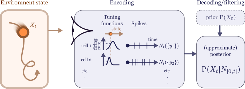
We assume that given $X_{t}=x$, points are generated independently of the past of $X$ and of previously generated points from all sensors. Each generated point is “marked” with the parameter $y_{i}$ of the sensor that generated it. We therefore describe the observations by a marked point process, i.e., a random counting measure $N$ on $[0,\infty)\times\mathcal{\mathbf{Y}}$ where $\mathbf{Y}$ is the mark space, and the observations available at time $t$ are the restriction of $N$ to the set $[0,t]\times\mathcal{\mathbf{Y}}$. Such a process may also be described as a vector of (unmarked) point processes, one for each sensor; however, we adopt the marked point process view to allow taking the limit of infinitely many sensors, as described below. Figure 1 illustrates this setting in a biological context, where the sensors are neurons and the points events are spikes (action potentials).

We denote by $f$ the counting measure of sensor marks over the mark space $\mathbf{Y}$, i.e., $f=\sum_{i}\delta_{y_{i}}$, where $\delta_{y}$ is the Dirac delta measure at $y$. Then the marked process $N_{t}$ has the measure-valued random process $\lambda_{t}\left(X_{t};y\right)f\left(dy\right)$ as its intensity kernel (see, e.g., [26], Chapter VIII), meaning that the rate (or intensity) of points with marks in a set $Y\subseteq\mathbf{Y}$ at time $t$ is

$$\sum_{i:y_{i}\in Y}\lambda_{t}\left(X_{t};y_{i}\right)=\int_{Y}\lambda_{t}\left(X_{t};y\right)f\left(dy\right).$$

Thus, the dynamics of $N$ may be described heuristically by means of the intensity kernel as

$$\mathrm{E}\left[N\left(dt,dy\right)|X_{\left[0,t\right]},N_{\left[0,t\right]}\right]=\lambda_{t}\left(X_{t};y\right)f\left(dy\right)dt.$$ (1)

Continuing the auditory example, the expected instantaneous total rate of spikes from all neurons which are tuned to a frequency within the range $\left[y_{\mathrm{min}},y_{\mathrm{max}}\right]$ (conditioned on the history of the external state and of neural firing) would be given by the integral of $\lambda_{t}\left(X_{t};y\right)f\left(dy\right)$ over this range of frequencies.

We generalize this model by allowing $f$ to be an arbitrary measure on $\mathbf{Y}$ (not necessarily discrete). A continuous measure may be useful as an approximate model for the response of a large number of sensors, which may be easier to analyze than its discrete counterpart. For example, a simplifying assumption in some previous works is that tuning curve centers are located on an equally-spaced grid (e.g., [23, 29, 30]). In the limit of infinitely many neurons, this is equivalent to taking $f$ to be the Lebesgue measure—the uniform “distribution” over the entire space.

2.2 Rigorous formulation

We now proceed to describe our model more rigorously. We assume the state $X_{t}\in\mathbb{R}^{n}$ obeys a Stochastic Differential Equation (SDE)

$$dX_{t}=A\left(X_{t}\right)dt+B\left(U_{t}\right)dt+D\left(X_{t}\right)dW_{t},\quad\left(t\geq 0\right),$$ (2)

where $A\left(\cdot\right),B\left(\cdot\right),D\left(\cdot\right)$ are arbitrary functions such that the SDE has a unique solution, $U$ is a control process and $W$ is a Wiener process. The initial condition $X_{0}$ is assumed to have a continuous distribution with a known density.

The observation process $N$ is a marked point process with marks from a measurable space $\left(\mathbf{Y},\mathcal{Y}\right)$, i.e., a random counting measure on $[0,\infty)\times\mathbf{Y}$. We use the notation $N_{t}\left(Y\right)\triangleq N\left([0,t]\times Y\right)$ for $Y\in\mathcal{Y}$, and when $Y=\mathbf{Y}$ we omit it and write simply $N_{t}$.

Denote by $\left(\Omega,\mathcal{F},P\right)$ the underlying probability space, and by $\mathcal{X},\mathcal{N}$ the filtrations generated by $X,N$ respectively, that is,

$$\mathcal{X}_{t} \triangleq\sigma\left(X_{\left[0,t\right]}\right)=\sigma\left\{X_{s}:s\leq t\right\}$$

$$\mathcal{N}_{t} \triangleq\sigma\left(N_{\left[0,t\right]\times\mathbf{Y}}\right)=\sigma\left\{N\left((a,b]\times Y\right):a<b\leq t,Y\in\mathcal{Y}\right\}$$

where $N_{\left[0,t\right]\times\mathbf{Y}}$ is the measure $N$ restricted to $\left[0,t\right]\times\mathbf{Y}$. We assume the control process $U$ is adapted to $\mathcal{N}$. Let $\mathcal{B}_{t}=\mathcal{X}_{t}\vee\mathcal{N}_{t}$ be the smallest $\sigma$-algebra containing $\mathcal{X}_{t}$ and $\mathcal{N}_{t}$. We assume that the process $N_{t}\left(Y\right)$ has an intensity kernel with respect to $\mathcal{B}$ given by $\lambda_{t}\left(X_{t};y\right)f\left(dy\right)$ for some known function $\lambda_{t}\left(x;y\right)$ and measure $f\left(dy\right)$ on $\mathcal{Y}$, meaning that for each $Y\in\mathcal{Y}$, $C_{t}^{Y}\triangleq\int_{0}^{t}\left(\int_{Y}\lambda_{s}\left(X_{s};y\right)f\left(dy\right)\right)ds$ is $\mathcal{B}_{t}$-predictable and $N_{t}\left(Y\right)-C_{t}^{Y}$ is a $\mathcal{B}_{t}$-martingale. This condition is the rigorous equivalent of (1) (see, e.g., [31] for a discussion of this definition in the unmarked case). Note in particular that the presence of feedback in (2), which may depend on the history of $N$, means that $N\left(Y\right)$ is not in general a doubly-stochastic Poisson process, which forces us to resort to a more sophisticated definition. Our results are applicable to this general setting, and not restricted in application to doubly-stochastic Poisson processes.

We define

$$\hat{\lambda}_{t}\left(y\right) \triangleq\mathrm{E}\left[\lambda_{t}\left(X_{t};y\right)|\mathcal{N}_{t}\right],$$

$$\hat{\lambda}_{t}^{f} \triangleq\int\hat{\lambda}_{t}\left(y\right)f\left(dy\right).$$

The measure $\hat{\lambda}_{t}\left(y\right)f\left(dy\right)$ is the intensity kernel of $N$ with respect to its natural filtration $\mathcal{N}$, i.e., $\int_{Y}\hat{\lambda}_{t}\left(y\right)f\left(dy\right)$ is the intensity of $N_{t}\left(Y\right)$ w.r.t. $\mathcal{N}$ for each $Y\in\mathcal{Y}$ (see [31], Theorem 2), and $\hat{\lambda}_{t}^{f}$ is the intensity of the unmarked process $N_{t}$. For $Y\in\mathcal{Y}$, the innovation process of $N_{t}\left(Y\right)$ is therefore $N_{t}\left(Y\right)-\int_{0}^{t}\int_{Y}\hat{\lambda}_{t}\left(y\right)f\left(dy\right)ds$, and accordingly we define the innovation measure $I$ by

$$I\left(dt,dy\right)\triangleq N\left(dt,dy\right)-\hat{\lambda}_{t}\left(y\right)f\left(dy\right)dt.$$ (3)

2.3 Encoding and decoding

We consider the question of optimal encoding and decoding under the above model. By decoding we mean computing (exactly or approximately) the full posterior distribution of $X_{t}$ given $\mathcal{N}_{t}$. The problem of optimal encoding is then the problem of optimal sensor configuration, i.e., finding the optimal rate function $\lambda_{t}\left(x;y\right)$ and population distribution $f\left(dy\right)$ so as to minimize some performance criterion. We assume the $\lambda_{t}\left(x;y\right)$ and $f\left(dy\right)$ come from some parameterized family with parameter $\phi$.

To quantify the performance of the encoding-decoding system, we summarize the result of decoding using a single estimator $\hat{X}_{t}=\hat{X}_{t}\left(\mathcal{N}_{t}\right)$, and define the Mean Square Error (MSE) as $\epsilon_{t}\triangleq\mathrm{trace}[(X_{t}-\hat{X}_{t})(X_{t}-\hat{X}_{t})^{T}]$. We seek $\hat{X}_{t}$ and $\phi$ that solve $\min_{\phi}\min_{\hat{X}_{t}}\mathrm{E}\left[\epsilon_{t}\right]=\min_{\phi}\mathrm{E}[\min_{\hat{X}_{t}}\mathrm{E}[\epsilon_{t}|\mathcal{N}_{t}]]$. The inner minimization problem in this equation is solved by the MSE-optimal decoder, which is the posterior mean $\hat{X}_{t}=\mu_{t}\triangleq\mathrm{E}\left[X_{t}|\mathcal{N}_{t}\right]$. The posterior mean may be computed from the full posterior obtained by decoding. The outer minimization problem is solved by the optimal encoder. Note that, although we assume a fixed parameter $\phi$ which does not depend on time, the optimal value of $\phi$ for which the minimum is obtained generally depends on the time $t$ where the error is to be minimized. In principle, the encoding/decoding problem can be solved for any value of $t$. In order to assess performance it is convenient to consider the steady-state limit $t\to\infty$ for the encoding problem.

Below, we approximately solve the decoding problem for any $t$, for some specific forms of $\lambda_{t}$ and $f$. We then explore the problem of choosing the steady-state optimal encoding parameters $\phi$ using Monte Carlo simulations in a biologically-motivated toy model. Note that if decoding is exact, the problem of optimal encoding becomes that of minimizing the expected posterior variance.

Having an efficient (closed-form) approximate filter allows performing the Monte Carlo simulation at a significantly reduced computational cost, relative to numerical methods such as particle filtering. The computational cost is further reduced by averaging the computed posterior variance across trials, rather than the squared error, thereby requiring fewer trials. The mean of the posterior variance equals the MSE (of the posterior mean), but has the advantage of being less noisy than the squared error itself – since by definition it is the mean of the square error under conditioning on $\mathcal{N}_{t}$ .

2.4 Special cases

To approximately solve the decoding problem in closed form, we focus on the case of Gaussian sensors: each sensor is marked with $y=\left(h,\theta,R\right)$ where $h\in\mathbb{R}_{+},\theta\in\mathbb{R}^{m}$, $R\in\mathbb{R}^{m\times m}$ is positive semidefinite, $m\leq n$, and

$$\lambda_{t}\left(x;h,\theta,R\right)=h\exp\left(-\frac{1}{2}\left\|Hx-\theta\right\|_{R}^{2}\right),$$ (4)

where $\left\|z\right\|_{M}^{2}\triangleq z^{T}Mz$, and $H\in\mathbb{R}^{m\times n}$ is a fixed matrix of full row rank, which maps the external state from $\mathbb{R}^{n}$ to “sensory coordinates” in $\mathbb{R}^{m}$. Here, $h$ is the tuning curve height, i.e., the maximum firing rate of the sensor; $\theta$ is the tuning curve center, i.e., the stimulus value in sensory coordinates which elicits the highest firing rate; and $R$ is the precision matrix of the Gaussian response curve in the sensory space $\mathbb{R}^{m}$. Following neuroscience terminology, we refer to the tuning curve center $\theta$ as the sensor’s preferred stimulus. The inclusion of the matrix $H$ allows using high-dimensional models where only some dimensions are observed, for example when the full state includes velocities but only locations are directly observable. In the one-dimensional case, $R^{-1/2}$ is the tuning curve width.

We consider several special forms of the population distribution $f$$\left(dh,d\theta,dR\right)$ where we can bring the approximate filter to closed form:

2.4.1 A single sensor

$f\left(dy\right)=\delta_{y}\left(dy\right)$, where $y=\left(h,\theta,R\right)$.

2.4.2 Uniform population

Here $h,R$ are fixed across all sensors, and $f\left(dh^{\prime},d\theta,dR^{\prime}\right)=\delta_{h}\left(dh^{\prime}\right)\delta_{R}\left(dR^{\prime}\right)d\theta$.

2.4.3 Gaussian population

Abusing notation slightly, we write $f\left(dh^{\prime},d\theta,dR^{\prime}\right)=\delta_{h}\left(dh^{\prime}\right)\delta_{R}\left(dR^{\prime}\right)f\left(d\theta\right)$ where

$$f\left(d\theta\right) =\mathcal{N}\left(\theta;c,\Sigma_{\mathrm{pop}}\right)d\theta$$

$$=\left(2\pi\right)^{-n/2}\left|\Sigma_{\mathrm{pop}}\right|^{-1/2}\exp\left(-\frac{1}{2}\left\|\theta-c\right\|_{\Sigma_{\mathrm{pop}}^{-1}}^{2}\right)d\theta,$$ (5)

for fixed $c\in\mathbb{R}^{m}$, and positive definite $\Sigma_{\mathrm{pop}}$.

We take $f$ to be normalized, since any scaling of $f$ may be included in the coefficient $h$ in (4), resulting in the same point-process. Thus, when used to approximate a large population of sensors, the coefficient $h$ would be proportional to the number of sensors.

2.4.4 Uniform population on an interval

In this case we assume a scalar state, $n=m=1$, and

$$f\left(d\theta\right) =1_{\left[a,b\right]}\left(\theta\right)d\theta,$$ (6)

where similarly to the Gaussian population case, $h$ and $R$ are fixed. Unlike the Gaussian case, here we find it more convenient not to normalize the distribution.

2.4.5 Finite mixtures

$f\left(dy\right)=\sum_{i}\alpha_{i}f_{i}\left(dy\right),$ where each $f_{i}$ is of one of the above forms. This form is quite general: it includes populations where $\theta$ is distributed according to a Gaussian mixture, as well as heterogeneous populations with finitely many different values of $R$. The resulting filter derived below includes a term for each component of the mixture.

3 Assumed Density Filtering

3.1 Exact filtering equations

Let $P\left(\cdot,t\right)$ denote the posterior density of $X_{t}$ given $\mathcal{N}_{t}$, and $\mathrm{E}_{P}^{t}\left[\cdot\right]$ the posterior expectation given $\mathcal{N}_{t}$. The prior density $P\left(\cdot,0\right)$ is assumed to be known.

The problem of filtering a diffusion process $X$ from a doubly stochastic Poisson process driven by $X$ is formally solved in [21]. The result is extended to general marked point processes in the presence of feedback in [23], where the authors derive a stochastic PDE for the posterior density, which in our setting takes the form

$$dP\left(x,t\right)= \mathcal{L}_{t}^{*}P\left(x,t\right)dt+P\left(x,t^{-}\right)\int_{y\in\mathbf{Y}}\frac{\lambda_{t^{-}}\left(x;y\right)-\hat{\lambda}_{t^{-}}\left(y\right)}{\hat{\lambda}_{t^{-}}\left(y\right)}I\left(dt,dy\right),$$ (7)

where $\mathcal{L}_{t}$ is the state’s posterior infinitesimal generator (Kolmogorov’s backward operator), defined as $\mathcal{L}_{t}f\left(x\right)=\lim_{\Delta t\to 0^{+}}\left(\mathrm{E}\left[f\left(X_{t+\Delta t}\right)|\mathcal{B}_{t}\right]-f\left(x\right)\right)/\Delta t$, $\mathcal{L}_{t}^{*}$ is $\mathcal{L}_{t}$’s adjoint operator (Kolmogorov’s forward operator), and $I$ is defined in (3). Expressions including $t^{-}$ are to be interpreted as left limits. Note that the discrete part of the measure $I\left(dt,dy\right)$, namely $N\left(dt,dy\right)$, contributes a discontinuous change in the posterior at each spike time. Also note that in this closed-loop setting, the infinitesimal generator is itself a random operator, due to its dependence on past observations through the control law.

The stochastic PDE (7) is non-linear and non-local (due to the dependence of $\hat{\lambda}_{t}\left(y\right)$ on $P\left(\cdot,t\right)$), and therefore usually intractable. In [23, 30] the authors consider linear dynamics with a Gaussian prior and Gaussian sensors with centers distributed uniformly over the state space. In this case, the posterior is Gaussian, and (7) leads to closed-form ODEs for its moments. In our more general setting, we can obtain exact equations for the posterior moments, as follows.

Let $\mu_{t}\triangleq\mathrm{E}_{P}^{t}X_{t},\tilde{X}_{t}\triangleq X_{t}-\mu_{t},\Sigma_{t}\triangleq\mathrm{E}_{P}^{t}[\tilde{X}_{t}\tilde{X}_{t}^{T}]$. Using (7), along with known results about the form of the infinitesimal generator $\mathcal{L}_{t}$ for diffusion processes (e.g. [32], Theorem 7.3.3), the first two posterior moments can be shown to obey the following equations:

$$d\mu_{t} =\left(\mathrm{E}_{P}^{t}\left[A\left(X_{t}\right)\right]+B\left(U_{t}\right)\right)dt+\int_{\mathbf{Y}}\mathrm{E}_{P}^{t-}\left[\omega_{t^{-}}\left(y\right)X_{t^{-}}\right]I\left(dt,dy\right)$$ (8)

$$d\Sigma_{t} =\mathrm{E}_{P}^{t}\left[A\left(X_{t\left(y\right)}\right)\tilde{X}_{t}^{T}+\tilde{X}_{t}A\left(X_{t}\right)^{T}+D\left(X_{t}\right)D\left(X_{t}\right)^{T}\right]dt$$

$$\quad+\int_{\mathbf{Y}}\mathrm{E}_{P}^{t^{-}}\left[\omega_{t^{-}}\left(y\right)\tilde{X}_{t^{-}}\tilde{X}_{t^{-}}^{T}\right]I\left(dt,dy\right)$$

$$\quad-\int_{\mathbf{Y}}\mathrm{E}_{P}^{t^{-}}\left[\omega_{t^{-}}\left(y\right)X_{t^{-}}\right]\mathrm{E}_{P}^{t^{-}}\left[\omega_{t^{-}}\left(y\right)X_{t^{-}}^{T}\right]N\left(dt,dy\right)$$ (9)

where

$$\omega_{t}\left(y\right)\triangleq\frac{\lambda_{t}\left(X_{t};y\right)}{\hat{\lambda}_{t}\left(y\right)}-1,$$

and similarly we write $\omega_{t}\left(x;y\right)\triangleq\lambda_{t}\left(x;y\right)/\hat{\lambda}_{t}\left(y\right)-1$.

In contrast with the more familiar LQG problem and the Kalman-Bucy filter, here the posterior variance is random, and is generally not monotonically decreasing even when estimating a constant state. However, noting that $\mathrm{E}\left[I\left(dt,dy\right)\right]=0$, we may observe from (9) that for a constant state ($A=D=0$), the expected posterior variance $\mathrm{E}\left[\Sigma_{t}\right]$ is decreasing.

Equations (8)-(9) are written in terms of the innovation process $I\left(dt,dy\right)$ and the original point process. Although this formulation highlights the relation to the Kalman-Bucy filter, we will find it useful to rewrite them in a different form, as follows,

$$d\mu_{t} =d\mu_{t}^{\pi}+d\mu_{t}^{\mathrm{c}}+d\mu_{t}^{N},$$

$$d\Sigma_{t} =d\Sigma_{t}^{\pi}+d\Sigma_{t}^{\mathrm{c}}+d\Sigma_{t}^{N},$$

where $d\mu_{t}^{\pi},d\Sigma_{t}^{\pi}$ are the prior terms, corresponding to $\mathcal{L}_{t}^{*}P\left(x,t\right)$ in (7), and the remaining terms are divided into continuous update terms $d\mu_{t}^{\mathrm{c}},d\Sigma_{t}^{\mathrm{c}}$ (multiplying $dt$) and discontinuous update terms $d\mu_{t}^{N},d\Sigma_{t}^{N}$ (multiplying $N\left(dt,dy\right)$). Using (3), we find

$$d\mu_{t}^{\pi} =\mathrm{E}_{P}^{t}\left[A\left(X_{t}\right)\right]dt+B\left(U_{t}\right)dt$$ (10)

$$d\Sigma_{t}^{\pi} =\mathrm{E}_{P}^{t}\left[A\left(X_{t}\right)\tilde{X}_{t}^{T}+\tilde{X}_{t}A\left(X_{t}\right)^{T}+D\left(X_{t}\right)D\left(X_{t}\right)^{T}\right]dt$$ (11)

$$d\mu_{t}^{\mathrm{c}} =-\int_{\mathbf{Y}}\mathrm{E}_{P}^{t}\left[\omega_{t}\left(y\right)X_{t}\right]\hat{\lambda}_{t}\left(y\right)f\left(dy\right)dt$$ (12)

$$d\Sigma_{t}^{\mathrm{c}} =-\int_{\mathbf{Y}}\mathrm{E}_{P}^{t}\left[\omega_{t}\left(y\right)\tilde{X}_{t}\tilde{X}_{t}^{T}\right]\hat{\lambda}_{t}\left(y\right)f\left(dy\right)dt$$ (13)

$$d\mu_{t}^{N} =\int_{\mathbf{Y}}\mathrm{E}_{P}^{t-}\left[\omega_{t^{-}}\left(y\right)X_{t^{-}}\right]N\left(dt,dy\right)$$ (14)

$$d\Sigma_{t}^{N} =\int_{\mathbf{Y}}\bigg{(}\mathrm{E}_{P}^{t^{-}}\left[\omega_{t^{-}}\left(y\right)\tilde{X}_{t^{-}}\tilde{X}_{t^{-}}^{T}\right]$$ (15)

$$\quad-\mathrm{E}_{P}^{t^{-}}\left[\omega_{t^{-}}\left(y\right)X_{t^{-}}\right]\mathrm{E}_{P}^{t^{-}}\left[\omega_{t^{-}}\left(y\right)X_{t^{-}}^{T}\right]\bigg{)}N\left(dt,dy\right).$$

The prior terms $d\mu_{t}^{\pi},d\Sigma_{t}^{\pi}$ represent the known dynamics of $X$, and are the same terms appearing in the Kalman-Bucy filter. These would be the only terms left if no measurements were available, and would vanish for a static state. The continuous update terms $d\mu_{t}^{\mathrm{c}},d\Sigma_{t}^{\mathrm{c}}$ represent updates to the posterior between spikes that are not derived from $X$’s dynamics, and therefore may be interpreted as corresponding to information obtained from the absence of spikes. The discontinuous update terms $d\mu_{t}^{N},d\Sigma_{t}^{N}$ contribute a change to the posterior at spike times, depending on the spike’s mark $y$, and thus represent information obtained from the presence of a spike as well as its associated mark.

Note that only the continuous update terms depend explicitly on the population distribution $f$. Discontinuous updates depend on the population distribution only indirectly through their influence on the statistics of the point process $N$.

3.2 ADF approximation

While equations (10)-(15) are exact, they are not practical, since they require computation of the full posterior $\mathrm{E}_{P}^{t}\left[\cdot\right]$. To bring them to a closed form, we use ADF with an assumed Gaussian density (see [18] for details). Informally, this may be envisioned as integrating (10)-(15) while replacing the distribution $P$ by its approximating Gaussian “at each time step”. The approximating Gaussian is obtained by matching the first two moments of $P$ [18]. Note that the solution of the resulting equations does not in general match the first two moments of the exact solution, though it may approximate it. Practically, the ADF approximation amounts to substituting the normal distribution $\mathcal{N}(x;\mu_{t},\Sigma_{t})$ for $P(x,t)$ to compute the expectations in (10)-(15).

If the dynamics are linear, the prior updates (10)-(11) are easily computed in closed form after this substitution. Otherwise, they may be approximated assuming the non-linear functions $A(x)$ and $D\left(x\right)D\left(x\right)^{T}$ may be written as power series, using well-known results about the moments of Gaussian vectors. The next sections are therefore devoted to the approximation of the non-prior updates (12)-(15).

3.3 Approximate form for Gaussian sensors

We now proceed to apply the Gaussian ADF approximation $P\left(x,t\right)\approx\mathcal{N}\left(x;\mu_{t},\Sigma_{t}\right)$ to (12)-(15) in the case of Gaussian sensors (4), deriving approximate filtering equations written in terms of the population density $f\left(dh,d\theta,dR\right)$. Abusing notation, from here on we use $\mu_{t},\Sigma_{t}$, and $P\left(x,t\right)$ to refer to the ADF approximation rather than to the exact values.

To evaluate the posterior of expectations in (12)-(15) we first simplify the expression

$$P\left(x,t\right)\omega_{t}\left(x;y\right)=\frac{P\left(x,t\right)\lambda_{t}\left(x;y\right)}{\int P\left(\xi,y\right)\lambda_{t}\left(\xi;y\right)d\xi}-P\left(x,t\right).$$ (16)

Using the Gaussian ADF approximation $P\left(x,t\right)=\mathcal{N}\left(x;\mu_{t},\Sigma_{t}\right)$ and (4), we find

$$P\left(x,t\right) \lambda_{t}\left(x;h,\theta,R\right)=$$

$$=h\mathcal{N}\left(x;\mu_{t},\Sigma_{t}\right)\exp\left(-\frac{1}{2}\left\|Hx-\theta\right\|_{R}^{2}\right)$$

$$=\frac{h\exp\left(-\frac{1}{2}\left\|x-\mu_{t}\right\|_{\Sigma_{t}^{-1}}^{2}-\frac{1}{2}\left\|Hx-\theta\right\|_{R}^{2}\right)}{\sqrt{\left(2\pi\right)^{n}\left|\Sigma_{t}\right|}}$$

$$=\frac{h}{\sqrt{\left(2\pi\right)^{n}\left|\Sigma_{t}\right|}}\exp\left(-\frac{1}{2}\left\|H_{r}^{-1}\theta-\mu_{t}\right\|_{Q_{t}^{R}}^{2}-\frac{1}{2}\left\|x-\mu_{t}^{\theta}\right\|_{\Sigma_{t}^{-1}+H^{T}RH}^{2}\right),$$

where $H_{r}^{-1}$ is any right inverse of $H$, and

$$Q_{t}^{R} \triangleq \Sigma_{t}^{-1}\left(\Sigma_{t}^{-1}+H^{T}RH\right)^{-1}H^{T}RH,$$

$$\mu_{t}^{\theta} \triangleq \left(\Sigma_{t}^{-1}+H^{T}RH\right)^{-1}\left(Q_{t}\mu_{t}+H^{T}R\theta\right).$$

An application of the Woodbury identity establishes the relation $Q_{t}^{R}=H^{T}S_{t}^{R}H$, where

$$S_{t}^{R}\triangleq\left(R^{-1}+H\Sigma_{t}H^{T}\right)^{-1},$$ (17)

yielding

$$P\left(x,t\right)\lambda_{t}\left(x;h,\theta,R\right)\\ \quad=\frac{h}{\sqrt{\left(2\pi\right)^{n}\left|\Sigma_{t}\right|}}\exp\left(-\frac{1}{2}\left\|\theta-H\mu_{t}\right\|_{S_{t}^{R}}^{2}-\frac{1}{2}\left\|x-\mu_{t}^{\theta}\right\|_{\Sigma_{t}^{-1}+H^{T}RH}^{2}\right),$$ (18)

and by normalizing this Gaussian (see (16)) we find that

$$P\left(x,t\right)\omega_{t}\left(x;h,\theta,R\right) =\mathcal{N}\left(x;\mu_{t}^{\theta},\left(\Sigma_{t}^{-1}+H^{T}RH\right)^{-1}\right)-P\left(x,t\right)$$

yielding

$$\mathrm{E}_{P}^{t}\left[\omega_{t}\left(h,\theta,R\right)X_{t}\right] =\mu_{t}^{\theta}-\mu_{t}$$

$$\mathrm{E}_{P}^{t}\left[\omega_{t}\left(h,\theta,R\right)\tilde{X}_{t}\tilde{X}_{t}^{T}\right] =\left(\Sigma_{t}^{-1}+H^{T}RH\right)^{-1}+\left(\mu_{t}-\mu_{t}^{\theta}\right)\left(\mu_{t}-\mu_{t}^{\theta}\right)^{T}-\Sigma_{t}.$$

Substituting the definition of $\mu_{t}^{\theta}$ and simplifying using the Woodbury identity yields

$$\mathrm{E}_{P}^{t} \left[\omega_{t}\left(h,\theta,R\right)X_{t}\right]=-\Sigma_{t}H^{T}S_{t}^{R}\left(H\mu_{t}-\theta\right),$$

$$\mathrm{E}_{P}^{t} \left[\omega_{t}\left(h,\theta,R\right)\tilde{X}_{t}\tilde{X}_{t}^{T}\right]=\Sigma_{t}H^{T}\left(S_{t}^{R}\left(H\mu_{t}-\theta\right)\left(H\mu_{t}-\theta\right)^{T}S_{t}^{R}-S_{t}^{R}\right)H\Sigma_{t}.$$

Plugging this result into (12)-(15) yields

$$d\mu_{t}^{\mathrm{c}} =\Sigma_{t}H^{T}\int_{\mathbf{Y}}S_{t}^{R}\left(H\mu_{t}-\theta\right)\hat{\lambda}_{t}\left(h,\theta,R\right)f\left(dh,d\theta,dR\right)dt$$ (19)

$$d\Sigma_{t}^{\mathrm{c}} =\Sigma_{t}H^{T}\int_{\mathbf{Y}}\left(S_{t}^{R}-S_{t}^{R}\left(H\mu_{t}-\theta\right)\left(H\mu_{t}-\theta\right)^{T}S_{t}^{R}\right)$$

$$\qquad\qquad\qquad\times\hat{\lambda}_{t}\left(h,\theta,R\right)f\left(dh,d\theta,dR\right)H\Sigma_{t}dt$$ (20)

$$d\mu_{t}^{N} =\Sigma_{t^{-}}H^{T}\int_{\mathbf{Y}}S_{t^{-}}^{R}\left(\theta-H\mu_{t^{-}}\right)N\left(dt,d\left[h,\theta,R\right]\right)$$ (21)

$$d\Sigma_{t}^{N} =-\Sigma_{t^{-}}H^{T}\int_{\mathbf{Y}}S_{t^{-}}^{R}N\left(dt,d\left[h,\theta,R\right]\right)H\Sigma_{t^{-}}$$ (22)

We also note that integrating (18) over $x$ yields

$$\hat{\lambda}_{t}\left(h,\theta,R\right) =h\sqrt{\frac{\left|S_{t}^{R}\right|}{\left|R\right|}}\exp\left(-\frac{1}{2}\left\|\theta-H\mu_{t}\right\|_{S_{t}^{R}}^{2}\right),$$ (23)

where we computed the coefficient using the equality $\left|I+\Sigma_{t}H^{T}RH\right|=\left|R\right|/\left|S_{t}^{R}\right|$, derived by application of Sylvester’s determinant identity.

To gain some insight into these equations, consider the case $H=I$. As seen from the discontinuous update equations (21)-(22), when a spike with mark $\left(h,\theta,R\right)$ occurs, the posterior mean moves towards the location mark $\theta$, and the posterior variance decreases (in the sense that $\Sigma_{t^{+}}-\Sigma_{t^{-}}$ is negative definite). Neither update depends on $h$.

In the scalar case $m=n=1$, with $H=1$, $\sigma_{t}^{2}=\Sigma_{t},\sigma_{\mathrm{r}}^{2}=R^{-1},a=A,d=D$, the discontinuous update equations (21)-(22) read

$$d\mu_{t}^{N} =\int_{\mathbf{Y}}\frac{\sigma_{t^{-}}^{2}}{\sigma_{t^{-}}^{2}+\sigma_{\mathrm{r}}^{2}}\left(\theta-\mu_{t^{-}}\right)N\left(dt,d\left[h,\theta,\sigma_{r}^{2}\right]\right)$$ (24)

$$d\Sigma_{t}^{N} =-\int_{\mathbf{Y}}\frac{\sigma_{t^{-}}^{2}}{\sigma_{t^{-}}^{2}+\sigma_{\mathrm{r}}^{2}}\sigma_{t^{-}}^{2}N\left(dt,d\left[h,\theta,\sigma_{r}^{2}\right]\right)$$ (25)

The continuous mean update equation (19) also admits an intuitive interpretation, in the case where all sensors share the same precision matrix $R$, i.e. $f\left(d\left[h,\theta,R^{\prime}\right]\right)=f\left(dh,d\theta\right)\delta_{R}\left(dR^{\prime}\right)$. In this case, the equation reads

$$d\mu_{t}^{\mathrm{c}} =\Sigma_{t}H^{T}S_{t}^{R}\left(H\mu_{t}-\int_{\mathbf{Y}}\theta\nu_{t}\left(\theta\right)f\left(dh,d\theta\right)\right)\hat{\lambda}_{t}^{f}dt$$

where $\nu_{t}\left(\theta\right)\triangleq\hat{\lambda}_{t}\left(h,\theta,R\right)/\hat{\lambda}_{t}^{f}$ (which does not depend on $h$). The normalized intensity kernel $\nu_{t}\left(\theta\right)f\left(dh,d\theta\right)$ may be interpreted heuristically as the distribution of the mark $\left(h,\theta\right)$ of the next event provided it occurs immediately. Thus, the absence of events drives the posterior mean away from the expected location of the next mark. The strength of this effect scales with $\hat{\lambda}_{t}^{f}$, which is the rate of the unmarked process $N_{t}$ w.r.t. its natural filtration, i.e., the total expected rate of spikes given the firing history. This behavior is qualitatively similar to the result obtained in [13] for a finite population of sensors observing a continuous-time finite-state Markov process, where the posterior probability between spikes concentrates on states with lower total firing rate.

3.4 Closed form approximations in special cases

Using (23), we now evaluate the continuous update equations (19)-(20) for the specific forms of the population distribution $f\left(dy\right)$ listed in section 2.4. Note that the discontinuous update equations (21)-(22) do not depend on the population distribution $f$, and are already in closed form.

3.4.1 Single sensor

The result for a single sensor with parameters $h,\theta,R$ is trivial to obtain from (19)-(20), yielding

$$d\mu_{t}^{\mathrm{c}} =\Sigma_{t}H^{T}S_{t}^{R}\left(H\mu_{t}-\theta\right)\hat{\lambda}_{t}^{f}dt,$$ (26)

$$d\Sigma_{t}^{\mathrm{c}} =\Sigma_{t^{-}}H^{T}\left(S_{t}^{R}-S_{t}^{R}\left(H\mu_{t}-\theta\right)\left(H\mu_{t}-\theta\right)^{T}S_{t}^{R}\right)\hat{\lambda}_{t}^{f}H\Sigma_{t^{-}}dt,$$ (27)

where $\hat{\lambda}_{t}^{f}=\hat{\lambda}_{t}\left(h,\theta,R\right)$ as given by (23), and $S_{t}^{R}$ is defined in (17).

3.4.2 Uniform population

Here all sensors share the same height $h$ and precision $R$, whereas the location parameter $\theta$ covers $\mathbb{R}^{m}$ uniformly, i.e. $f\left(d\theta\right)=d\theta$. A straightforward calculation from (19)-(20) and (23) yields

$$d\mu_{t}^{\mathrm{c}} =0,\quad d\Sigma_{t}^{\mathrm{c}}=0,$$ (28)

in agreement with the (exact) result obtained in [23], where the filtering equations only include the prior term and the discontinuous update term.

3.4.3 Gaussian population

Here $R,h$ are constant, and $f\left(d\theta\right)$ is given in (5). Using (23),

$$\hat{\lambda}_{t}\left(h,\theta,R\right)f\left(d\theta\right) =h\sqrt{\frac{\left|S_{t}^{R}\right|}{\left|R\right|}}\exp\left(-\frac{1}{2}\left\|\theta-H\mu_{t}\right\|_{S_{t}^{R}}^{2}\right)\mathcal{N}\left(\theta;c,\Sigma_{\mathrm{pop}}\right)d\theta.$$

An analogous computation to the derivation of (18) and (23) above yields

$$\hat{\lambda}_{t}\left(h,\theta,R\right)f\left(d\theta\right) =\hat{\lambda}_{t}^{f}\cdot\mathcal{N}\left(\theta;\mu_{t}^{f},\left(\Sigma_{\mathrm{pop}}^{-1}+S_{t}^{R}\right)^{-1}\right)d\theta,$$

$$\hat{\lambda}_{t}^{f} =\int\hat{\lambda}_{t}\left(h,\theta,R\right)f\left(d\theta\right)$$

$$=h\sqrt{\frac{\left|Z_{t}^{R}\right|}{\left|R\right|}}\exp\left(-\frac{1}{2}\left\|c-H\mu_{t}\right\|_{Z_{t}^{R}}^{2}\right)$$ (29)

where

$$Z_{t}^{R} \triangleq\left(\Sigma_{\mathrm{pop}}+\left(S_{t}^{R}\right)^{-1}\right)^{-1}=\left(\Sigma_{\mathrm{pop}}+R^{-1}+H\Sigma_{t}H^{T}\right)^{-1}$$ (30)

$$\mu_{t}^{f} \triangleq\left(\Sigma_{\mathrm{pop}}^{-1}+S_{t}^{R}\right)^{-1}\left(S_{t}^{R}\mu_{t}+\Sigma_{\mathrm{pop}}^{-1}c\right).$$

Substituting into (19)-(20) and simplifying yields the following continuous update equations

$$d\mu_{t}^{\mathrm{c}} =\Sigma_{t}H^{T}Z_{t}^{R}\left(H\mu_{t}-c\right)\hat{\lambda}_{t}^{f}dt$$ (31)

$$d\Sigma_{t}^{\mathrm{c}} =\Sigma_{t}H^{T}\Big{(}Z_{t}^{R}-Z_{t}^{R}\left(H\mu_{t}-c\right)\left(H\mu_{t}-c\right)^{T}Z_{t}^{R}\Big{)}H\Sigma_{t}\hat{\lambda}_{t}^{f}dt,$$ (32)

where $Z_{t}^{R}$ and $\hat{\lambda}_{t}^{f}$ are given by (30) and (29), respectively. These updates generalize the single-sensor updates (26)-(27), with the population center $c$ taking the place of the single location parameter, and $Z_{t}^{R}$ substituting $S_{t}^{R}$. The single sensor case is obtained when $\Sigma_{\mathrm{pop}}=0$.

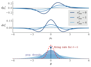
It is illustrative to consider these equations in the scalar case $m=n=1$, with $H=1$. Letting $\sigma_{t}^{2}=\Sigma_{t},\sigma_{\mathrm{r}}^{2}=R^{-1},\sigma_{\mathrm{pop}}^{2}=\Sigma_{\mathrm{pop}}$ yields

$$d\mu_{t}^{\mathrm{c}} =\frac{\sigma_{t}^{2}}{\sigma_{t}^{2}+\sigma_{\mathrm{r}}^{2}+\sigma_{\mathrm{pop}}^{2}}\left(\mu_{t}-c\right)\hat{\lambda}_{t}^{f}dt,$$ (33)

$$d\sigma_{t}^{2,\mathrm{c}} =\frac{\sigma_{t}^{2}}{\sigma_{t}^{2}+\sigma_{\mathrm{r}}^{2}+\sigma_{\mathrm{pop}}^{2}}\left(1-\frac{\left(\mu_{t}-c\right)^{2}}{\sigma_{t}^{2}+\sigma_{\mathrm{r}}^{2}+\sigma_{\mathrm{pop}}^{2}}\right)\sigma_{t}^{2}\hat{\lambda}_{t}^{f}dt,$$ (34)

where

$$\hat{\lambda}_{t}^{f}=h\sqrt{2\pi\sigma_{\mathrm{r}}^{2}}\mathcal{N}\left(\mu_{t};c,\sigma_{t}^{2}+\sigma_{\mathrm{r}}^{2}+\sigma_{\mathrm{pop}}^{2}\right).$$

Figure 2a demonstrates the continuous update terms (33)-(34) as a function of the current mean estimate $\mu_{t}$, for various values of the population variance $\sigma_{\mathrm{pop}}^{2}$, including the case of a single sensor, $\sigma_{\mathrm{pop}}^{2}=0$. The continuous update term $d\mu_{t}^{\mathrm{c}}$ pushes the posterior mean $\mu_{t}$ away from the the population center $c$ in the absence of spikes. This effect weakens as $\left|\mu_{t}-c\right|$ grows due to the factor $\hat{\lambda}_{t}^{f}$, consistent with the idea that far from $c$, the lack of events is less surprising, hence less informative. The continuous variance update term $d\sigma_{t}^{2,\mathrm{c}}$ increases the variance when $\mu_{t}$ is near $\theta$, otherwise decreases it. This stands in contrast with the Kalman-Bucy filter, where the posterior variance cannot increase when estimating a static state.

(a) Gaussian population ((33)-(34)). Parameters are $c=0,\sigma_{\mathrm{r}}^{2}=0.25,h=1,\sigma_{t}^{2}=1$. The case $\sigma_{\mathrm{pop}}^{2}=0$ corresponds to a single sensor.

(b) Uniform population on an interval ((35)-(36)). Parameters are $\left[a,b\right]=\left[-1,1\right],h=1,\sigma_{t}^{2}=0.01$.

Figure 2: Continuous update terms as a function of the current posterior mean estimate, for a 1-d state observed through a population of Gaussian sensors (4). The population density is Gaussian on the left plot, and uniform on the interval $\left[-1,1\right]$ on the right plot. The bottom plots shows the population density $f\left(d\theta\right)/d\theta$ and a tuning curve $\lambda_{t}\left(x;\theta\right)$ for $\theta=0$.

3.4.4 Uniform population on an interval

In this case $R,h$ are constant, and $f\left(d\theta\right)$ is given in (6). Here we assume $m=n=1$ and $H=1$, so (19)-(20) take the form

$$d\mu_{t}^{\mathrm{c}} =\frac{\sigma_{t}^{2}}{\sigma_{t}^{2}+\sigma_{\mathrm{r}}^{2}}\int_{\theta\in\mathbb{R}}\left(\mu_{t}-\theta\right)\hat{\lambda}_{t}\left(\theta\right)f\left(d\theta\right)dt$$

$$d\sigma_{t}^{2,\mathrm{c}} =\left(\hat{\lambda}_{t}^{f}-\frac{\int\left(\theta-\mu_{t}\right)^{2}\hat{\lambda}_{t}\left(\theta\right)f\left(d\theta\right)}{\sigma_{t}^{2}+\sigma_{\mathrm{r}}^{2}}\right)\frac{\sigma_{t}^{2}}{\sigma_{t}^{2}+\sigma_{\mathrm{r}}^{2}}\sigma_{t}^{2}dt$$

$$\hat{\lambda}_{t}\left(\theta\right) =h\sqrt{2\pi\sigma_{\mathrm{r}}^{2}}\mathcal{N}\left(\theta;\mu_{t},\sigma_{\mathrm{r}}^{2}+\sigma_{t}^{2}\right),$$

where $\sigma_{t}^{2}=\Sigma_{t},\sigma_{\mathrm{r}}^{2}=R^{-1}$, and we suppressed the dependence of $\hat{\lambda}$ on $h,R$ from the notation, since $h,R$ are fixed. Let $\phi\left(x\right)=\mathcal{N}\left(x;0,1\right),\Phi\left(x\right)=\int_{-\infty}^{x}\phi$. A straightforward computation using the moments of the truncated Gaussian distribution yields

$$\hat{\lambda}_{t}^{f}=\int_{a}^{b}\hat{\lambda}_{t}\left(\theta\right)d\theta =h\sqrt{2\pi\sigma_{\mathrm{r}}^{2}}Z_{t},$$

$$\int\left(\theta-\mu_{t}\right)\hat{\lambda}_{t}\left(\theta\right)f\left(d\theta\right) =-h\sqrt{2\pi\sigma_{\mathrm{r}}^{2}}z_{t}\sqrt{\sigma_{t}^{2}+\sigma_{\mathrm{r}}^{2}},$$

$$\int\left(\theta-\mu_{t}\right)^{2}\hat{\lambda}_{t}\left(\theta\right)f\left(d\theta\right) =\left[\hat{\lambda}_{t}^{f}-h\sqrt{2\pi\sigma_{\mathrm{r}}^{2}}z^{\prime}_{t}\right]\left(\sigma_{t}^{2}+\sigma_{\mathrm{r}}^{2}\right),$$

where

$$\alpha_{t} =\frac{a-\mu_{t}}{\sqrt{\sigma_{t}^{2}+\sigma_{\mathrm{r}}^{2}}}\,, Z_{t} =\Phi\left(\beta_{t}\right)-\Phi\left(\alpha_{t}\right),$$

$$\beta_{t} =\frac{b-\mu_{t}}{\sqrt{\sigma_{t}^{2}+\sigma_{\mathrm{r}}^{2}}}\,, z_{t} =\phi\left(\beta_{t}\right)-\phi\left(\alpha_{t}\right),$$

$$z^{\prime}_{t} =\beta_{t}\phi\left(\beta_{t}\right)-\alpha_{t}\phi\left(\alpha_{t}\right),$$

yielding

$$d\mu_{t}^{\mathrm{c}} =h\sqrt{2\pi\sigma_{\mathrm{r}}^{2}}\sqrt{\frac{\sigma_{t}^{2}}{\sigma_{t}^{2}+\sigma_{\mathrm{r}}^{2}}}z_{t}\sigma_{t}dt$$ (35)

$$d\sigma_{t}^{2,\mathrm{c}} =h\sqrt{2\pi\sigma_{\mathrm{r}}^{2}}\frac{\sigma_{t}^{2}}{\sigma_{t}^{2}+\sigma_{\mathrm{r}}^{2}}z^{\prime}_{t}\sigma_{t}^{2}dt$$ (36)

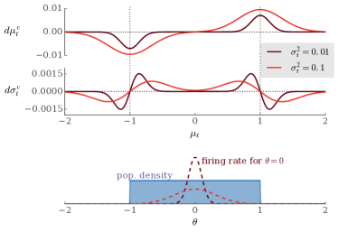
Figure 2b demonstrates the continuous update terms (35)-(36) as a function of the current mean estimate $\mu_{t}$. When the mean estimate is around an endpoint of the interval, the mean update $\mu_{t}^{\mathrm{c}}$ pushes the posterior mean outside the interval in the absence of spikes. The posterior variance $\sigma_{t}^{2}$ decreases outside the interval, where the absence of spikes is expected, and increases inside the interval, where it is unexpected. When the posterior mean is not near the interval endpoints, the updates are near zero, consistently with the uniform population case (28).

3.4.5 Finite Mixtures

Assume $f$ is any finite mixture of measures

$$f\left(dy\right)=\sum_{i}\alpha_{i}f_{i}\left(dy\right),$$

where $f_{i}$ is of one of the above forms. We note that the continuous updates (12)-(13) are linear in $f$, so they are obtained by the appropriate weighted sums of the filters derived above for the various special forms of $f_{i}$.

In particular, for a general mixture of the first three forms,

$$f\left(dh,dR,d\theta\right) =\sum_{i}\alpha_{i}^{\delta}\delta_{h_{i}}\left(dh\right)\delta_{R_{i}}\left(dR\right)\delta_{\theta_{i}}\left(d\theta\right)$$

$$\quad+\sum_{i}\alpha_{i}^{U}\delta_{h_{i}^{U}}\left(dh\right)\delta_{R_{i}^{U}}\left(dR\right)d\theta$$

$$\quad+\sum_{i}\alpha_{i}^{\mathcal{N}}\delta_{h_{i}^{\mathcal{N}}}\left(dh\right)\delta_{R_{i}^{\mathcal{N}}}\left(dR\right)\mathcal{N}\left(\theta;c_{i},\Sigma_{\mathrm{pop}}^{\left(i\right)}\right)d\theta,$$

the resulting continuous update terms are given by

$$d\mu_{t}^{\mathrm{c}}=\Sigma_{t}H^{T}\Bigg{(} \sum_{i}\alpha_{i}^{\delta}S_{t}^{i}\left(H\mu_{t}-\theta_{i}\right)\hat{\lambda}_{t}\left(h_{i},\theta_{i},R_{i}\right)$$

$$\qquad+ \sum_{i}\alpha_{i}^{\mathcal{N}}Z_{t}^{i}\left(H\mu_{t}-c_{i}\right)\hat{\lambda}_{t}^{f,i}\bigg{)}dt,$$

$$d\Sigma_{t}^{\mathrm{c}}=\Sigma_{t}H^{T}\Bigg{\{} \sum_{i}\alpha_{i}^{\delta}\left[S_{t}^{i}-S_{t}^{i}\left(H\mu_{t}-\theta_{i}\right)\left(H\mu_{t}-\theta_{i}\right)^{T}S_{t}^{i}\right]\hat{\lambda}_{t}\left(h_{i},\theta_{i},R_{i}\right)$$

$$+\sum_{i}\alpha_{i}^{\mathcal{N}}\left[Z_{t}^{i}-Z_{t}^{i}\left(H\mu_{t}-c_{i}\right)\left(H\mu_{t}-c_{i}\right)^{T}Z_{t}^{i}\right]\hat{\lambda}_{t}^{f,i}\Bigg{\}}H\Sigma_{t}dt,$$

where $\hat{\lambda}_{t}\left(h,\theta,R\right)$ is given by (23), $S_{t}^{i}=S_{t}^{R_{i}},Z_{t}^{i}=Z_{t}^{R_{i}^{\mathcal{N}}}$ as defined in (17),(30), and similarly,

$$\hat{\lambda}_{t}^{f,i}=h_{i}^{\mathcal{N}}\sqrt{\frac{\left|Z_{t}^{i}\right|}{\left|R_{i}^{\mathcal{N}}\right|}}\exp\left(-\frac{1}{2}\left\|c_{i}-H\mu_{t}\right\|_{Z_{t}^{i}}^{2}\right)$$

(cf. (29)). The uniform components of the mixture do not appear explicitly in the filter, since the continuous update part vanishes for the uniform case (see (28)), though they would influence the discontinuous update terms through their effect on the statistics of $N$.

4 Evaluation of filter

4.1 Examples and comparison to particle filter

(a) high rate of events: $h=1000$

(b) low rate of events: $h=2$

Figure 3: Two examples of a linear one-dimensional process observed through a Gaussian population (5) of Gaussian sensors (4), filtered using the ADF approximation (namely, equations (10)-(11),(19)-(20),(31)-(32)), and using a particle filter. Each dot correspond to a spike with the vertical location indicating the sensor’s location parameter $\theta$. The approximate posterior means obtained from ADF and particle filtering are shown in blue and red respectively, with the corresponding posterior standard deviations in shaded areas of the respective colors. The curves to the right of the graph show the preferred stimulus density (black), and a sensor’s response rate function (4) centered at $\theta=0$ (gray), arbitrarily normalized to the same height for visualization. The bottom graph shows the posterior variance. Parameters used in both examples: $a=-0.1,d=1,H=1,\sigma_{\mathrm{pop}}^{2}=4,R^{-1}=0.25,c=0,\mu_{0}=0,\sigma_{0}^{2}=1$ (note the different extent of the time axis). The observed processes were initialized from their steady-state distribution. The dynamics were discretized with time step $\Delta t=10^{-3}$. The particle filter uses 1000 particles with systematic resampling (see, e.g., [7]) at each time step.

Since the filter (10)-(15) is based on an assumed density approximation, its results may be inexact. We tested the accuracy of the filter in the Gaussian population case (31)-(32), by numerical comparison with Particle Filtering (PF) [7].

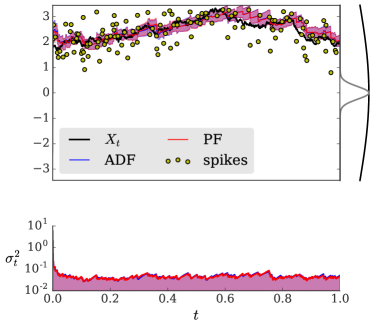
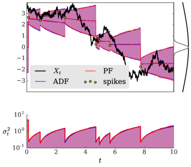
Figure 3 shows two examples of filtering a one-dimensional process observed through a Gaussian population of Gaussian sensors (5), using both the ADF approximation (33)-(34) and a Particle Filter (PF) for comparison. See the figure caption for precise details.

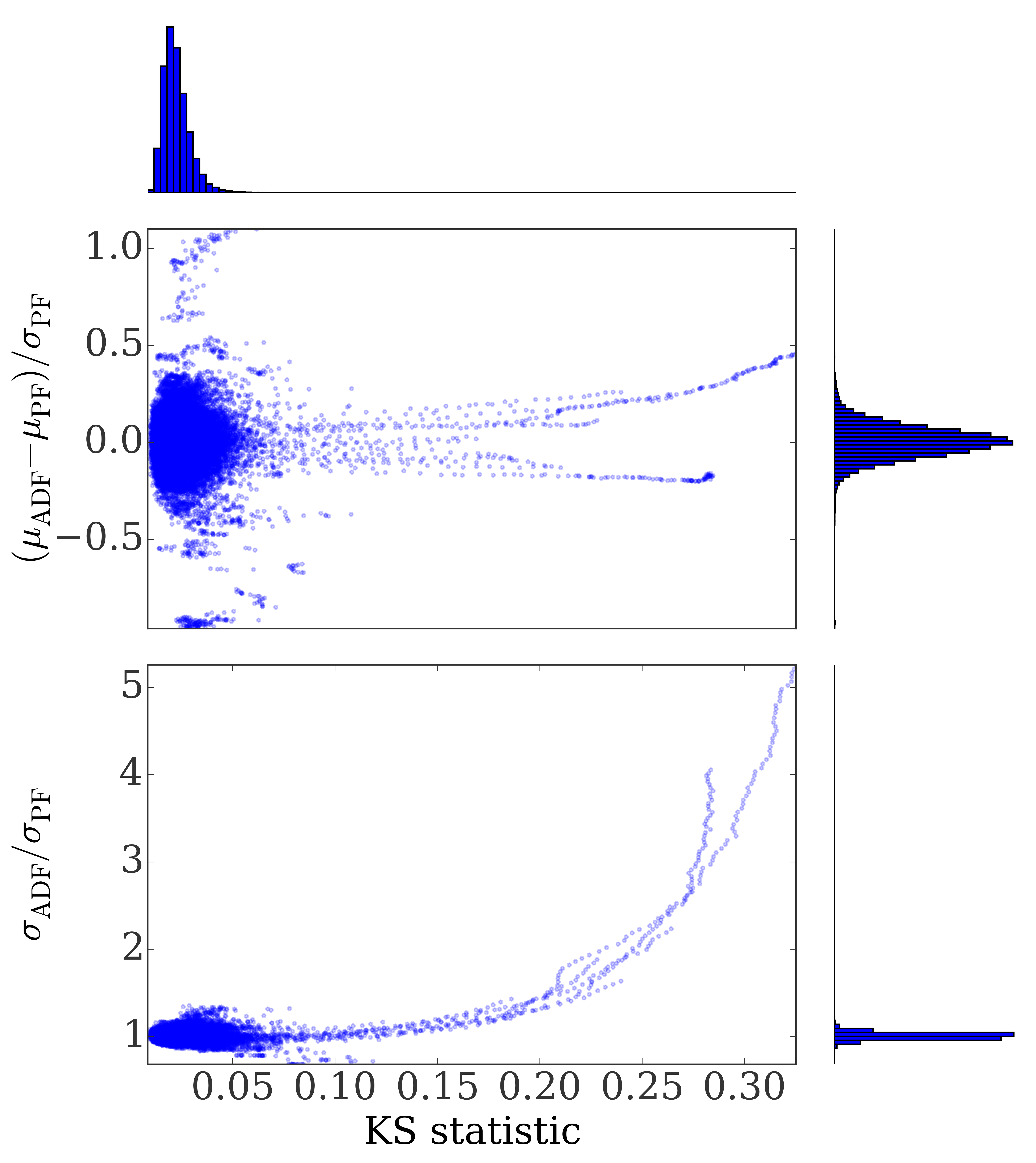
Figure 4 shows the distribution of approximation errors and their relation to the deviation of the posterior from Gaussian. The deviation of the particle distribution from Gaussian is quantified using the Kolmogorov-Smirnov (KS) statistic $\sup_{x}\left|F\left(x\right)-G\left(x\right)\right|$ where $F$ is the particle distribution cdf and $G$ is the cdf of a Gaussian matching $F$’s first two moments. The approximation errors plotted are the relative error in the mean estimate $\epsilon_{\mu}\triangleq\left(\mu_{\mathrm{ADF}}-\mu_{\mathrm{PF}}\right)/\sigma_{\mathrm{PF}}$, and the error in the posterior standard deviation estimate $\epsilon_{\sigma}\triangleq\sigma_{\mathrm{ADF}}/\sigma_{\mathrm{PF}}$, where $\mu_{\mathrm{ADF}},\mu_{\mathrm{PF}},\sigma_{\mathrm{ADF}},\sigma_{\mathrm{PF}}$ are, respectively, the posterior mean obtained from ADF and PF, and the posterior variance obtained from ADF and PF. The observed mean and standard deviation of the estimation errors are $0.0018\pm 0.0989$ for $\epsilon_{\mu}$ and $1.010\pm 0.101$ for $\epsilon_{\sigma}$. The results suggest that the largest errors occur in rare cases where the posterior diverges significantly from Gaussian, and involve an overestimation of the posterior variance. Similar results were obtained with different parameters.

Figure 4: Approximation errors (relative to particle filter) vs. KS statistic of particle distribution. The KS statistic is plotted against the estimation errors $\epsilon_{\mu},\epsilon_{\sigma}$ (see main text). Each point corresponds to a single simulation time step. The histograms show the distribution of the KS statistic, of $\epsilon_{\mu}$ and of $\epsilon_{\sigma}$. Results obtained from 100 trials of length $T=1$, with parameters as in Figure 3a.

4.2 Information gained between spikes

The filters derived above for various population distributions differ only in the continuous update terms, which modify the posterior between spikes beyond the prior terms derived from the state dynamics. We may therefore interpret this term as corresponding to information gained by the absence of spikes. The continuous update term vanishes in the uniform population filter of [23] (see (28)), so that in the uniform case, between spikes the posterior dynamics are identical to the prior dynamics. This reflects the fact that lack of spikes in a time interval is an indication that the total firing rate is low; in the uniform population case, this is not informative, since the total firing rate is independent of the state.

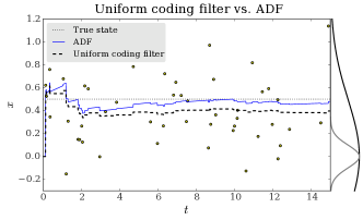
Figure 5 (left) illustrates the contribution of the continuous update terms (31)-(32) to filter performance. A static scalar state is observed by a Gaussian population (4)-(5), and filtered twice: once with the correct value of $\sigma_{\mathrm{pop}}^{2}=\Sigma_{\mathrm{pop}}$, and once with $\sigma_{\mathrm{pop}}\rightarrow\infty$, which yields $\mu_{t}^{\mathrm{c}}=0$, recovering the uniform population filter of [23]. Between spikes, the ADF estimate moves away from the population center $c=0$, whereas the uniform coding estimate remains fixed. The size of this effect decreases with time, as the posterior variance estimate (not shown) decreases. The reduction in filtering errors gained from the continuous update terms is illustrated in Figure 5 (right). Despite the approximation involved, the full filter significantly outperforms the uniform population filter. The difference disappears as $\sigma_{\mathrm{pop}}$ increases and the population becomes uniform.

Figure 5: Left Illustration of information gained between spikes. A static state $X_{t}=0.5$, shown in a dotted line, is observed by a Gaussian population (5) of Gaussian sensors (4), and filtered twice: with the correct value $\sigma_{\mathrm{pop}}^{2}=0.5$ (“ADF”, solid blue line), and with $\sigma_{\mathrm{pop}}^{2}=\infty$ (“Uniform coding filter”, dashed line), which is equivalent to ignoring the continuous update terms. Both filters are applied to the same random realization of the observation process. The curves to the right of each graph show the preferred stimulus density (black), and a tuning curve centered at $\theta=0$ (gray). Both filters are initialized with $\mu_{0}=0,\sigma_{0}^{2}=1$. Right Comparison of MSE for the ADF filter and the uniform coding filter. The vertical axis shows the integral of the square error integrated over the time interval $\left[5,10\right]$, averaged over 1000 trials. Shaded areas indicate estimated errors, computed as the sample standard deviation divided by the square root of the number of trials. Parameters in both plots are $a=d=0,c=0,\sigma_{\mathrm{pop}}^{2}=0.5,\sigma_{\mathrm{r}}^{2}=0.1,H=1,h=10$.

5 Encoding

5.1 Motivation

We demonstrate the use of the Assumed Density Filter in determining optimal encoding strategies, i.e., selecting the optimal sensor population parameters $\phi$ (see Section 2.3 above). The study of optimal encoding has both biological and engineering motivations. In the context of neuroscience, the optimal encoding strategy may serve as a model for the observed characteristics of sensory neurons, or for observed sensory adaptation (e.g., [8]). Several works have studied optimal neural encoding using Fisher information as a performance criterion. Fisher information is easily computed from tuning functions in the case of static state (e.g., [8]), and this approach completely circumvents the need to model the decoding process. For example, in [33], the authors consider a scalar static state observed by a parameterized population of neurons, and analytically optimize the parameters based on Fisher information under a constraint on the total expected rate of spikes. A few works (e.g. [29, 30]) consider the more difficult problem of direct minimization of the MSE rather than the Fisher information, by solving the corresponding filtering problem and measuring the MSE of different encoding parameters using Monte Carlo (MC) simulations. The filtering problem is made tractable in [29] and [30] by assuming a uniform population (equivalent to case 2 in Section 2.4) above. However, sensory populations are often non-uniform (e.g. [34]), and sensory adaptation often modifies tuning curves non-uniformly (e.g. [11]), which motivates our more general setting. Optimization of sensor configuration and coding is also increasingly studied in engineering contexts (e.g., [35, 36, 37, 38]), as networked filtering and control are becoming ubiquitous. The latter studies are usually concerned with continuous observations (often linear), rather than PP based observations using heterogeneous biologically motivated tuning functions as is done here.

5.2 Encoding example

To illustrate the use of ADF for the encoding problem, we consider a simple example using a Gaussian population (5). We will study optimal encoding issues in more detail in a sequel paper.

Previous work using a finite neuron population and a Fisher information-based criterion [12] has suggested that the optimal distribution of preferred stimuli depends on the prior variance. When it is small relative to the tuning curve width, optimal encoding is achieved by placing all preferred stimuli at a fixed distance from the prior mean. On the other hand, when the prior variance is large relative to the tuning curve width, optimal encoding is uniform (see figure 2 in [12]). These results are consistent with biological observations reported in [34] concerning the encoding of aural stimuli.

Similar results are obtained with our model, as shown in Figure 6. Whereas [12] implicitly assumed a static state in the computation of Fisher information, we use a time-varying scalar state. The state obeys the dynamics

$$dX_{t}=aX_{t}dt+d\,dW_{t}\quad\left(a<0\right),$$

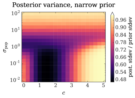
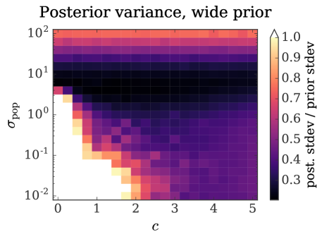
and is observed through a Gaussian population (5) and filtered using the ADF approximation. In this case, optimal encoding is interpreted as the simultaneous optimization of the population center $c$ and the population variance $\Sigma_{\mathrm{pop}}$. The process is initialized so that it has a constant prior distribution, its variance given by $d^{2}/\left(2\left|a\right|\right)$. In Figure 6 (left), the steady-state prior distribution is narrow relative to the tuning curve width, leading to an optimal population with a narrow population distribution far from the origin. In Figure 6 (right), the prior is wide relative to the tuning curve width, leading to an optimal population with variance that roughly matches the prior variance.

Our approach, though more computationally expensive, offers two advantages over the Fisher information-based method which is used in [12] and which is prevalent in computational neuroscience. First, the simple computation of Fisher information from tuning curves, commonly used in the neuroscience literature, is based on the assumption of a static state, whereas our method can be applied in a fully dynamic context, including the presence of observation-dependent feedback. Second, our approach allows the minimization of arbitrary criteria, including the direct minimization of posterior variance or Mean Square Error (MSE). Although, under appropriate conditions, Fisher information approaches the MSE in the limit of infinite decoding time, it may be a poor proxy for the MSE for finite decoding times (e.g., [39, 29]), which are of particular importance in natural settings and in control problems.

Figure 6: Optimal population distribution depends on prior variance relative to tuning curve width. A scalar state with dynamics $dX_{t}=aX_{t}+d\,dW_{t}$ ($a=-0.05$) is filtered with tuning curves parameters $h=50,\sigma_{\mathrm{r}}=1$ and preferred stimulus density $\mathcal{N}(c,\sigma_{\mathrm{pop}}^{2})$. The process is initialized from its steady state distribution, $\mathcal{N}\left(0,d^{2}/\left(-2a\right)\right)$. Both graphs show the posterior standard deviation derived from the ADF approximation, relative to the prior standard deviation $\sigma_{\mathrm{p}}$. In the left graph, $d=0.1$ so that the prior variance is $0.1$, whereas on the right, $d=1$, so that the prior variance is $10$. In both cases the filter is initialized with the correct prior, and the posterior variance is averaged over the time interval $\left[1,2\right]$ and across 1000 trials for each data point. Only non-negative values of $c$ were simulated, but note that the process is symmetric about zero, so that the full plots would also be symmetric about $c=0$. The areas colored in white in the right plot correspond to parameters where the computed posterior variance exceeded the prior variance. This is due to poor performance of the ADF approximation for these parameter values, in cases where no spikes occur and the true posterior becomes bimodal.

6 Conclusions

We have introduced an analytically tractable approximation to point process filtering, allowing us to gain insight into the generally intractable infinite-dimensional filtering problem. The approach enables the derivation of near-optimal encoding schemes going beyond the previously studied case of uniform population. The framework is presented in continuous time, circumventing temporal discretization errors and numerical imprecision in sampling-based methods, applies to fully dynamic setups, and directly estimates the MSE rather than lower bounds to it. It successfully explains observed experimental results, and opens the door to many future predictions. Moreover, the proposed strategy may lead to practically useful decoding of spike trains.

References

- [1] B. Anderson and J. Moore, Optimal Filtering. Dover, 2005.
- [2] R. Kalman and R. Bucy, “New results in linear filtering and prediction theory,” J. of Basic Eng., Trans. ASME, Series D, vol. 83(1), pp. 95–108, 1961.
- [3] R. Kalman, “A new approach to linear filtering and prediction problems,” J. Basic Eng., Trans. ASME, Series D., vol. 82(1), pp. 35–45, 1960.
- [4] F. Daum, “Nonlinear filters: beyond the kalman filter,” Aerospace and Electronic Systems Magazine, IEEE, vol. 20, no. 8, pp. 57–69, 2005.
- [5] S. Julier, J. Uhlmann, and H. Durrant-Whyte, “A new method for the nonlinear transformation of means and covariances in filters and estimators,” IEEE Trans. Autom. Control, vol. 45(3), pp. 477–482, 2000.
- [6] I. Arasaratnam and S. Haykin, “Cubature kalman filters,” IEEE Transactions on automatic control, vol. 54, no. 6, pp. 1254–1269, 2009.
- [7] A. Doucet and A. Johansen, “A tutorial on particle filtering and smoothing: fifteen years later,” in Handbook of Nonlinear Filtering, D. Crisan and B. Rozovskii, Eds. Oxford, UK: Oxford University Press, 2009, pp. 656–704.
- [8] P. Dayan and L. Abbott, Theoretical Neuroscience: Computational and Mathematical Modeling of Neural Systems. MIT Press, 2005.
- [9] A. Benucci, D. L. Ringach, and M. Carandini, “Coding of stimulus sequences by population responses in visual cortex.” Nature neuroscience, vol. 12, no. 10, pp. 1317–1324, 2009.
- [10] Y. Gutfreund, W. Zheng, and E. Knudsen, “Gated visual input to the central auditory system.” Science, vol. 297, no. 5586, pp. 1556–9, Aug 2002, 449 (Tech).
- [11] A. Benucci, A. B. Saleem, and M. Carandini, “Adaptation maintains population homeostasis in primary visual cortex.” Nature neuroscience, vol. 16, no. 6, pp. 724–9, 2013.
- [12] N. Harper and D. McAlpine, “Optimal neural population coding of an auditory spatial cue.” Nature, vol. 430, no. 7000, pp. 682–686, Aug 2004, n1397b.
- [13] O. Bobrowski, R. Meir, and Y. Eldar, “Bayesian filtering in spiking neural networks: noise, adaptation, and multisensory integration.” Neural Comput, vol. 21, no. 5, pp. 1277–1320, May 2009.
- [14] A. Susemihl, R. Meir, and M. Opper, “Analytical results for the error in filtering of gaussian processes,” in Advances in Neural Information Processing Systems 24, J. Shawe-Taylor, R. Zemel, P. Bartlett, F. Pereira, and K. Weinberger, Eds., 2011, pp. 2303–2311.
- [15] ——, “Dynamic state estimation based on poisson spike trains—towards a theory of optimal encoding,” Journal of Statistical Mechanics: Theory and Experiment, vol. 2013, no. 03, p. P03009, 2013.
- [16] P. Maybeck, Stochastic Models, Estimation, and Control. Academic Press, 1979.
- [17] D. Brigo, B. Hanzon, and F. LeGland, “A differential geometric approach to nonlinear filtering: the projection filter,” Automatic Control, IEEE Transactions on, vol. 43, pp. 247–252, 1998.
- [18] M. Opper, “A Bayesian approach to online learning,” in Online Learning in Neural Networks, D. Saad, Ed. Cambridge university press, 1998, pp. 363–378.
- [19] T. Minka, “Expectation propagation for approximate bayesian inference,” in Proceedings of the Seventeenth conference on Uncertainty in artificial intelligence. Morgan Kaufmann Publishers Inc., 2001, pp. 362–369.
- [20] A. Susemihl, “Optimal population coding of dynamic stimuli,” Ph.D. dissertation, Technical University Berlin, 2014.
- [21] D. Snyder, “Filtering and detection for doubly stochastic Poisson processes,” IEEE Transactions on Information Theory, vol. 18, no. 1, pp. 91–102, Jan. 1972.
- [22] A. Segall, “Recursive estimation from discrete-time point processes,” Information Theory, IEEE Transactions on, vol. 22, no. 4, pp. 422–431, 1976.
- [23] I. Rhodes and D. Snyder, “Estimation and control performance for space-time point-process observations,” IEEE Transactions on Automatic Control, vol. 22, no. 3, pp. 338–346, 1977.
- [24] D. Snyder, I. Rhodes, and E. Hoversten, “A separation theorem for stochastic control problems with point-process observations,” Automatica, vol. 13, no. 1, pp. 85–87, 1977.
- [25] A. Segall, “Centralized and decentralized control schemes for Gauss-Poisson processes,” IEEE Transactions on Automatic Control, vol. 23, no. 1, pp. 47–57, 1978.
- [26] P. Brémaud, Point Processes and Queues: Martingale Dynamics. Springer, New York, 1981.
- [27] R. Frey and W. J. Runggaldier, “A nonlinear filtering approach to volatility estimation with a view towards high frequency data,” International Journal of Theoretical and Applied Finance, vol. 4, no. 02, pp. 199–210, 2001.
- [28] Y. Harel, R. Meir, and M. Opper, “A tractable approximation to optimal point process filtering: Application to neural encoding,” in Advances in Neural Information Processing Systems, 2015, pp. 1603–1611.
- [29] S. Yaeli and R. Meir, “Error-based analysis of optimal tuning functions explains phenomena observed in sensory neurons.” Front Comput Neurosci, vol. 4, p. 130, 2010.
- [30] A. Susemihl, R. Meir, and M. Opper, “Optimal Neural Codes for Control and Estimation,” Advances in Neural Information Processing Systems, pp. 1–9, 2014.
- [31] A. Segall and T. Kailath, “The modeling of randomly modulated jump processes,” Information Theory, IEEE Transactions on, vol. 21, no. 2, pp. 135–143, 1975.
- [32] B. Øksendal, Stochastic Differential Equations. Springer, 2003.
- [33] D. Ganguli and E. Simoncelli, “Efficient sensory encoding and bayesian inference with heterogeneous neural populations.” Neural Comput, vol. 26, no. 10, pp. 2103–2134, 2014.
- [34] A. Brand, O. Behrend, T. Marquardt, D. McAlpine, and B. Grothe, “Precise inhibition is essential for microsecond interaural time difference coding.” Nature, vol. 417, no. 6888, pp. 543–547, 2002.
- [35] S. Yüksel and T. Başar, Stochastic networked control systems: Stabilization and optimization under information constraints. Springer Science & Business Media, 2013.
- [36] B. R. Andrievsky, A. S. Matveev, and A. L. Fradkov, “Control and estimation under information constraints: Toward a unified theory of control, computation and communications,” Automation and Remote Control, vol. 71, no. 4, pp. 572–633, 2010.
- [37] A. I. Mourikis and S. I. Roumeliotis, “Optimal sensor scheduling for resource-constrained localization of mobile robot formations,” IEEE Transactions on Robotics, vol. 22, no. 5, pp. 917–931, Oct 2006.
- [38] J. L. Ny, E. Feron, and M. A. Dahleh, “Scheduling continuous-time kalman filters,” IEEE Transactions on Automatic Control, vol. 56, no. 6, pp. 1381–1394, June 2011.
- [39] M. Bethge, D. Rotermund, and K. Pawelzik, “Optimal short-term population coding: when fisher information fails.” Neural Comput, vol. 14, no. 10, pp. 2317–2351, Oct 2002.