Impact of axisymmetric mass models for dwarf spheroidal galaxies on indirect dark matter searches

Abstract

Dwarf spheroidals are low-luminosity satellite galaxies of the Milky Way highly dominated by dark matter (DM). Therefore, they are prime targets to search for signals from dark matter annihilation using gamma-ray observations. While the typical assumption is that the dark matter density profile of these satellite galaxies can be described by a spherical symmetric Navarro-Frenk-White (NFW) profile, recent observational data of stellar kinematics suggest that the DM halos around these galaxies are better described by axisymmetric profiles. Motivated by such evidence, we analyse about seven years of PASS8 Fermi data for seven classical dwarf galaxies, including Draco, adopting both the widely used NFW profile and observationally-motivated axisymmetric density profiles. For four of the selected dwarfs (Sextans, Carina, Sculptor and Fornax) axisymmetric mass models suggest a cored density profile rather than the commonly adopted cusped profile. We found that upper limits on the annihilation cross section for some of these dwarfs are significantly higher than the ones achieved using an NFW profile. Therefore, upper limits in the literature obtained using spherical symmetric cusped profiles, such as the NFW, might be overestimated. Our results show that it is extremely important to use observationally motivated density profiles going beyond the usually adopted NFW in order to obtain accurate constraints on the dark matter annihilation cross section.

I Introduction

Most of the matter in the Universe consists of an unknown component that is commonly considered to be made of non-baryonic cold dark matter 2011ApJS..192…18K ; Ade:2015xua . Finding the particle nature of dark matter (DM) is one of the most pressing goals in modern physics. While many particle physics models have been proposed to solve this puzzle, the most favored and extensively studied candidates fall into the category of weakly interacting massive particles (WIMPs) 2005PhR…405..279B . These are characterised by a relic density matching the observed DM density, and naturally arise in many theories beyond the standard model of particle physics such as supersymmetry or universal extra-dimension models. The self-annihilation of WIMPs can result in the production of standard model particles. The goal of so-called indirect DM searches is to look for these particles in regions of the Universe where we know DM is abundant Gaskins:2016cha .

High-energy gamma rays are one example of those particles expected as a result of WIMP annihilation. The search for these gamma rays is a very active field of research fueled in the last decade by many gamma-ray observations of Milky Way (MW) satellite galaxies 2009ApJ…697.1299A ; 2010ApJ…720.1174A ; 2011JCAP…06..035A ; 2011PhRvL.107x1302A ; 2012PhRvD..85f2001A ; 2014JCAP…02..008A ; Abdo:2010ex ; Ackermann:2013yva ; 2014PhRvD..90k2012A ; Geringer-Sameth:2014qqa ; Ackermann:2015zua ; Geringer-Sameth:2015lua ; 2015ApJ…809L…4D ; 2016JCAP…02..039M ; PhysRevD.93.043518 and other promising sites such as the Galactic center 2011PhRvL.106p1301A ; 2011PhRvD..84l3005H ; 2015PhRvL.114h1301A ; 2015JCAP…03..038C ; 2016PDU….12….1D ; 2015PhRvD..91f3003C ; 2016ApJ…819…44A ; Zhou:2014lva or clusters of galaxies 2010ApJ…710..634A ; 2010JCAP…05..025A ; 2012ApJ…750..123A ; 2012JCAP…07..017A ; 2012ApJ…757..123A ; 2015ApJ…812..159A ; 2016JCAP…02..026A ; PhysRevD.93.103525 , both from the ground with imaging Cherenkov telescopes and from space with the Fermi Large Area Telescope (LAT). More recently, novel and competitive constraints have been obtained also from the Fermi measurements of the extragalactic gamma-ray background 2012PhRvD..85h3007A ; 2013MNRAS.429.1529F ; 2013PhRvD..87l3539A ; 2014PhRvD..90b3514A ; 2014NIMPA.742..149G ; 2015PhR…598….1F ; 2015ApJS..221…29C ; 2015JCAP…06..029C ; 2015ApJ…802L…1F ; Regis:2015zka ; Ando:2016ang ; Fornasa:2016ohl .

In this paper, we focus on dwarf spheroidal galaxies (dSphs) that are low-luminosity satellite galaxies which are known to be highly DM dominated 1998ARA&A..36..435M ; 2007PhRvD..75h3526S ; 2008ApJ…678..614S ; 2011JCAP…12..011S ; Chiappo:2016xfs . Their high mass-to-light ratio, proximity, and very low expected gamma-ray background from other astrophysical sources make them ideal candidates to search for gamma rays from DM annihilation. The main astrophysical uncertainty when dealing with indirect DM searches in dSphs is their DM density profile, which is the most crucial ingredient needed to estimate the rate of DM annihilation we expect from a given object. The common assumption often adopted in the literature is that dSphs are characterised by a spherically symmetric, so-called Navarro-Frenk-White (NFW) profile Navarro:1996gj . This cusped profile originally predicted by $N$-body simulations of cold dark matter might not be the best choice for all cases, and other profiles have been extensively discussed in the literature, including the Einasto profile 1965TrAlm…5…87E .

Additional complications come from going beyond simple spherical symmetric mass models. We know, in fact, that the observed stellar components of all MW dSphs have an axisymmetric shape on the sky-plane with typical axial ratios of 0.6–0.8 2012AJ….144….4M . Additionally, recent high-resolution $N$-body simulations showed that DM subhalos tend to have axisymmetric shapes rather than triaxial 2014MNRAS.439.2863V . These considerations prove the need to relax the assumption of spherical symmetry in the mass modeling of dSphs, which is also one of the major systematic uncertainties for the $J$-factor (i.e., the line-of-sight integral of DM density squared) estimations that most of previous studies have not considered.

In this paper we investigate the impact of observationally motivated axisymmetric mass models on indirect DM searches with dSphs using gamma-ray observations by Fermi. Uncertainties on the J-factor estimates were addressed in Ref. Ullio:2016kvy , where they explore the impact of the observationally unknown star orbital anisotropy. Triaxial density profiles have been investigated in detail in Ref. Bonnivard:2014kza , where they determine the bias on the $J$-factor that arises when using a spherical Jeans analysis for halos that are likely to be triaxial in shape. In our work, we go beyond the $J$-factor estimates and study the impact on the upper limits obtained for the DM cross section when adopting the axisymmetric models of Ref. Hayashi:2015yfa with respect to those obtained using the commonly adopted NFW profile. We analyse about seven years of PASS8 Fermi-LAT data for seven classical dSphs, namely Draco, Leo I and II, Sextans, Carina, Sculptor, and Fornax. These dSphs are selected as the overlapping part of the samples considered by Ref. Hayashi:2015yfa and Ref. Ackermann:2015zua . We fit each dSph both with NFW and axisymmetric profiles, and compare their cross section upper limits. We underline, in particular, that Sextans, Carina, Sculptor and Fornax are characterised by cored axisymmetric profiles rather than cusped, and their results can differ significantly from those of the NFW profiles.

This paper is organised as follows. In Sec. II, we discuss the expected flux from DM annihilation from dSphs in the case of a NFW profile. The axisymmetric mass model is introduced in Sec. III, where we also discuss a qualitative comparison with the NFW profile. In Sec. IV, we discuss the Fermi-LAT data analysis for the seven selected dSphs and present our results in Sec. V. We discuss our conclusions in Section VI.

II Gamma rays from dark matter annihilation

The gamma-ray intensity (i.e., the number of photons received per unit area, time, energy, and solid angle) from a direction $\psi$ relative to the center of the halo, expected from DM annihilation can be written as

$$\phi_{\text{WIMP}}(E,\psi)=J(\psi)\Phi^{\text{PP}}(E),$$ (1)

where $J(\psi)$ is the astrophysical factor, also called $J$-factor, which describes the DM density distribution in the region of interest, and $\Phi^{\text{PP}}(E)$ is the particle physics factor, which encloses the properties of the DM particle.

The particle physics factor can be written as

$$\Phi^{\text{PP}}(E)=\frac{1}{2}\frac{\langle\sigma v\rangle}{4\pi\,m^{2}_{\text{WIMP}}}\sum_{f}\frac{dN_{f}}{dE}B_{f},$$ (2)

where $m_{\text{WIMP}}$ is the WIMP mass, $\langle\sigma v\rangle$ is the the annihilation cross section multiplied by the relative velocity of the annihilating particles averaged over their velocity distribution, and $dN_{f}/dE$ is the photon spectrum of the final state $f$ with its branching ratio $B_{f}$.

The astrophysical $J$-factor is

$$J(\psi)=\int_{\text{l.o.s.}}\rho^{2}(l,\psi)\,dl,$$ (3)

where $l$ is the line-of-sight parameter, and $\rho(l,\psi)$ is the DM density profile. As mentioned in Sec. I, in our analysis of the Fermi-LAT data we compare the observationally-motivated axisymmetric DM density profile with the widely used spherically-symmetric NFW profile. The current section concerns the latter.

The NFW profile is given by Navarro:1996gj

$$\rho(r)=\left\{\begin{array}[]{lr}\frac{\rho_{s}r_{s}^{3}}{r(r_{s}+r)^{2}}&\text{for}\;\;r<r_{t}\\ 0&\text{for}\;\;r\geq r_{t}\end{array},\right.$$ (4)

where $\rho_{s}$ is the characteristic density, $r_{s}$ is the scale radius, and $r_{t}$ is the tidal radius beyond which all the DM particles are stripped away due to a strong tidal force from the host halo. We calculate the values for $\rho_{s}$ and $r_{s}$ from the parameters $v_{\text{max}}$ and $r_{\text{max}}$ provided by 2015MNRAS.451.2524M using the following relations:

$$r_{s} =\frac{r_{\text{max}}}{2.163}\;,$$ (5)

$$\rho_{s} =\frac{4.625}{4\pi G}\left(\frac{v_{\text{max}}}{r_{s}}\right)^{2},$$ (6)

where $G$ is the gravitational constant. We then derive $r_{t}$ from the Jacobi limit 1987Binney ,

$$r_{t}=D\left(\frac{M_{\text{dSph}}}{3M_{\text{MW}}}\right)^{\frac{1}{3}},$$ (7)

where $M_{\text{dSph}}$ is the mass of the dSph and $D$ is the distance of the dSph from the MW center. $M_{\text{MW}}$ is the MW mass enclosed within the distance $D$, calculated assuming an NFW profile from Ref. Colafrancesco:2006he . $M_{\text{dSph}}$ is calculated integrating the dSph NFW profile up to $r_{t}$, and we eventually solve equation (7) to obtain $r_{t}$. Note that the tidal radius calculated in this way is subject to various uncertainties connected to the mass estimate of the Milky Way and to several assumptions made for simplicity, such as a perfect circular orbit of the dSph around the stable MW potential. However, typically about $90$% of the annihilation flux comes from within $r_{s}$ for an NFW profile (see, e.g., 2011JCAP…12..011S ) and, therefore, variations on the tidal radius will only have little effects on the resulting J-factor. The main characteristics of each considered dSph are reported in Table 1.

Table 1: Characteristics of the analysed dwarf spheroidal galaxies. The top ones are cusped while bottom ones are cored in the axisymmetric mass modeling. The distances are taken from Ref. Ackermann:2015zua .

Name	Distance	$\rho_{s}$	$r_{s}$	$r_{t}$	NFW $J$-factor		axisymmetric $J$-factor
					total	$<0.5^{\circ}$	total	$<0.5^{\circ}$
	[kpc]	[$M_{\odot}\text{kpc}^{-3}$]	[kpc]	[kpc]	[GeV2 cm-5 sr]	[GeV2 cm-5 sr]	[GeV2 cm-5 sr]	[GeV2 cm-5 sr]
Draco	76	$2.30\times 10^{8}$	0.3507	0.96	$8.33\times 10^{18}$	$8.24\times 10^{18}$	$9.43\times 10^{18}$	$8.71\times 10^{18}$
Leo I	254	$1.59\times 10^{8}$	0.4027	6.26	$5.06\times 10^{17}$	$5.05\times 10^{17}$	$3.95\times 10^{17}$	$3.94\times 10^{17}$
Leo II	233	$1.83\times 10^{8}$	0.3055	4.73	$3.32\times 10^{17}$	$3.32\times 10^{17}$	$3.18\times 10^{17}$	$3.17\times 10^{17}$
Carina	105	$3.04\times 10^{8}$	0.2065	3.39	$1.50\times 10^{18}$	$1.49\times 10^{18}$	$2.61\times 10^{18}$	$2.36\times 10^{18}$
Fornax	147	$1.33\times 10^{8}$	0.4731	5.30	$1.83\times 10^{18}$	$1.81\times 10^{18}$	$1.67\times 10^{18}$	$1.52\times 10^{18}$
Sculptor	86	$1.67\times 10^{8}$	0.3935	3.25	$4.91\times 10^{18}$	$4.79\times 10^{18}$	$6.75\times 10^{18}$	$5.76\times 10^{18}$
Sextans	86	$3.82\times 10^{8}$	0.2018	1.55	$3.37\times 10^{18}$	$3.37\times 10^{18}$	$2.03\times 10^{18}$	$1.24\times 10^{18}$

Equation (3) yields the $J$-factor as a function of the angle between the line of sight and the center of the dSph. We project this onto a spatial map of $100\times 100$ pixels of $0.1^{\circ}$ centered on each dSph. These will be the template input for the Fermi-LAT data analysis of each dSph that is described in Sec. IV. We show the obtained NFW template maps in Figs. 1 and 2, where the total flux is normalized to unity.

Our reference works for the gamma-ray limits on dSph are those of Refs. Ackermann:2013yva ; Ackermann:2015zua . However, while Refs. Ackermann:2013yva ; Ackermann:2015zua limit their analysis within $0.5^{\circ}$ of each dSph, we do not limit the emission region in our analysis. Our choice is motivated by the fact that we want to compare the upper limits on the DM cross section obtained when adopting the NFW profiles against those obtained when adopting axisymmetric ones. As we will discuss in detail in the next section, the axisymmetric profiles are typically more extended compared to the NFW profiles. In Table 1, we show the total $J$-factor together with the one calculated within a radius of $0.5^{\circ}$ both for the NFW and the axisymmetric profiles. While for the NFW profiles the differences are insignificant, with maxima of about 1 and 2.5% for Draco and Sculptor, respectively, the differences in the case of the axisymmetric mass models are much more severe in most cases, except for Leo I and II. In particular, in the case of Sextans, about $40\%$ of the total axisymmetric J-factor would be ignored by considering only a region within $0.5^{\circ}$. Therefore, in order to have a consistent comparison between the NFW and the axisymmetric profiles, we do not limit the emission region of our dSphs in the data analysis and use $r_{t}$ as outermost radius in the generation of the template input maps for the NFW case.

Finally, note that our NFW $J$-factors do not necessary have to coincide with those of Refs. Ackermann:2013yva ; Ackermann:2015zua as they use the method of Ref. 2015MNRAS.451.2524M applied to stellar kinematics data to obtain their $J$-factors, while we use directly the $v_{\text{max}}$ and $r_{\text{max}}$ provided by Ref. 2015MNRAS.451.2524M . Nevertheless, our total $J$-factors integrated up to $r_{t}$ are always within the quoted errors of the $J$-factors from Refs. Ackermann:2013yva ; Ackermann:2015zua , with the notable exception of Leo II where ours is almost a factor of 2 smaller. With this exception in mind, we expect the limits that we calculate for NFW profiles to be comparable to those of Refs. Ackermann:2013yva ; Ackermann:2015zua , except for the fact that here we consider events from a larger energy range.

III Axisymmetric Mass Models

Our aim is to compare the constraints obtained using an NFW density profile to those obtained by using the observationally-motivated axisymmetric density profile. For the axisymmetric model, we use the non-spherical DM halo structure estimated by Ref. Hayashi:2015yfa to compute the $J$-factor maps. In this section, we briefly introduce the mass models based on the axisymmetric Jeans equations, the method of exploring the best-fit DM halo parameters, and the fitting results (for more details, we refer the reader to the original papers Hayashi:2015yfa ; Hayashi:2016 ).

Assuming that the stellar tracers in the dSphs are in dynamical equilibrium with a gravitational smooth potential dominated by DM, the distribution function obeys the steady-state collisionless Boltzmann equation 2008gady.book…..B . Given that both the stellar and DM components are axisymmetric, the axisymmetric Jeans equations can be derived from this equation by computing its velocity moments. When the distribution functions are of the form $f(E,L_{z})$, where $E$ and $L_{z}$ are the energy and the angular momentum along the symmetry axis $z$ respectively, the mixed moments vanish and the velocity dispersion of stars in cylindrical coordinates, $\overline{v^{2}_{R}}$ and $\overline{v^{2}_{z}}$, are identical; i.e., the velocity anisotropy parameter $\beta_{z}=1-\overline{v^{2}_{z}}/\overline{v^{2}_{R}}$ is exactly zero. However, since in general these velocity second moments are not identical, Ref. Hayashi:2015yfa adopted Cappellari’s formalism that relaxed $\overline{v^{2}_{R}}=\overline{v^{2}_{z}}$ and assumed $\beta_{z}={\rm constant}$ 2008MNRAS.390…71C . In addition, they assumed that the dSph stars did not rotate, and therefore the velocity second moment was equivalent to the velocity dispersion.

Under these assumptions, the axisymmetric Jeans equations are written as

$$\overline{v^{2}_{z}} = \frac{1}{\nu(R,z)}\int^{\infty}_{z}\nu\frac{\partial\Phi}{\partial z}dz,$$ (8)

$$\overline{v^{2}_{\phi}} = \frac{1}{1-\beta_{z}}\Biggl{[}\overline{v^{2}_{z}}+\frac{R}{\nu}\frac{\partial(\nu\overline{v^{2}_{z}})}{\partial R}\Biggr{]}+R\frac{\partial\Phi}{\partial R},$$ (9)

where $\nu$ is the three-dimensional stellar density profile and $\Phi$ is the gravitational potential. In order to compare them with the observed velocity second moments, the above equations should be integrated along the line of sight. Following the method given in Ref. 2006MNRAS.371.1269T , we computed the projected velocity second moments from $\overline{v^{2}_{R}}$, $\overline{v^{2}_{\phi}}$, and $\overline{v^{2}_{z}}$, taking into account the inclination of each dSph with respect to the observer. For the stellar and DM halo density models, which are related to $\nu$ and $\Phi$, we adopted an axisymmetric Plummer profile 1911MNRAS..71..460P (see Eq. 3 in Hayashi:2015yfa ) and an axisymmetric double power-law form (see Eq. 4 in Hayashi:2015yfa ), respectively.

Comparing the line-of-sight velocity moment profiles from theory and observations, Ref. Hayashi:2015yfa estimated the best-fit free parameters by using a Markov Chain Monte Carlo fitting method. There is a total of six free parameters in this model: the axial ratio, characteristic density and scale radius of the DM halo, the inner slope of the DM profile, the velocity anisotropy parameter and the inclination angle of the dSph. Applying their models to the available data of the seven MW dSphs (Carina, Fornax, Sculptor, Sextans, Draco, Leo I and Leo II), two important outcomes were found. First, while Leo I and Leo II have almost spherical dark halos, the other dSphs (Carina, Fornax, Sculptor, Sextans and Draco) are likely to have very flattened and oblate DM halos, with axial ratios of $\sim$0.4, even though there is a degeneracy between the axial ratio of the dark halo and the constant velocity anisotropy parameter. For example, the axisymmetric model for Sextans is preferred over a spherical symmetric one at around $2\sigma$ confidence level. Second, not all the DM halos in the dSphs have a cusped central density profile. Most of the dSphs indicate cored density profiles or shallow cusps. Exceptions are Draco and Leo I, which show a cusped profile with inner density slopes of $-0.86\pm 0.11$ and $-1.40^{+0.06}_{-0.08}$ respectively. The best-fit parameters of each dSph are summarized in Table 2 of Ref. Hayashi:2015yfa . We use these parameters to compute the sky distribution of the $J$-factors for Draco, Leo I, Leo II, Sextans, Carina, Sculptor and Fornax.

Figures 1 and 2 show both the NFW and axisymmetric density profiles projected onto the sky for the seven adopted dSphs.These are the spatial templates that are used in the Fermi-LAT data analysis of Sec. IV.The total flux in these maps is normalised to unity, and the colour scale of each pair NFW-axisymmetric is set to be the same, thus showing the relative size and brightness of the two models for a given dSph. As explained in the previous sections, when generating these template maps, the outermost radius is taken to be $r_{t}$ for the case of the NFW profiles. In the case of the axisymmetric profiles, for which $r_{t}$ values are not estimated within the framework of Ref. Hayashi:2015yfa , there is no formal limit to the radial extent of the profiles in the template maps. We stress, however, that as in both cases most of the annihilation flux comes from the inner parts, even though with the due differences (see Table 1), the choice of the outermost radial extent has no impact on our results.

Figure 1 shows the dSphs with a cusped density profile. For Leo I and Leo II, there is almost no visible difference between the NFW and the axisymmetric profiles projected onto the sky. For Draco, the shape of the axisymmetric model is oblate instead of spherical and clearly differs from the classical NFW, but still shows a cuspy. The differences between the two profiles are larger for the cored dSphs as can be seen in Fig. 2. In this case, the axisymmetric profiles are much more extended than the NFW profiles, with the total integrated $J$-factor being of the same order of magnitude, but distributed over a larger area (see also Table 1). Note also that these axisymmetric profiles are all oblate and characterised by different directions of the major axis following the stellar kinematics data for a given dSph. We will show that the case of the cored dSphs is the most affected by the simplification of adopting the NFW profile when obtaining DM constraints.

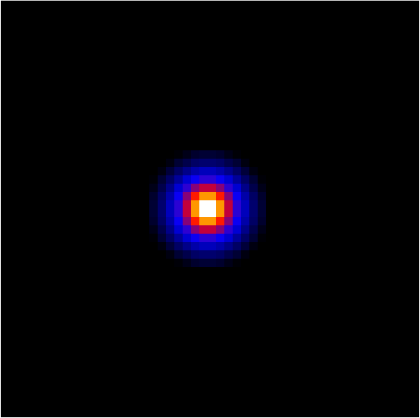
(a) Draco NFW

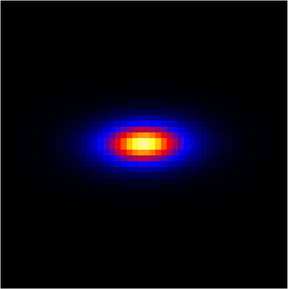
(b) Draco axisymmetric

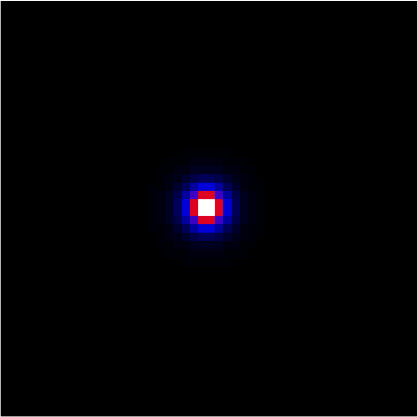
(c) Leo I NFW

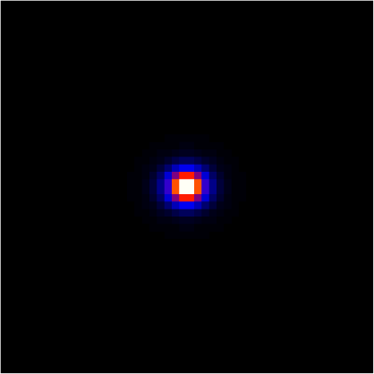
(d) Leo I axisymmetric

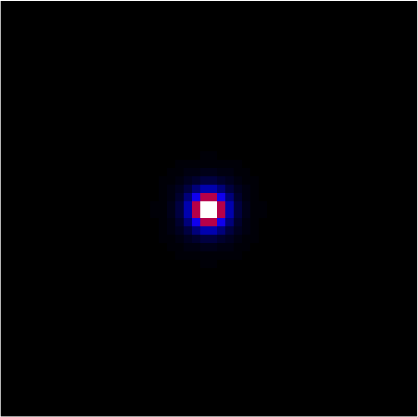
(e) Leo II NFW

(f) Leo II axisymmetric

Figure 1: DM density profiles projected onto the sky for the dSphs that have a cusped halo profile in log scale. From top to bottom, Draco, Leo I and Leo II, where the NFW profiles are shown on the left, and the axisymmetric profiles are shown on the right. The total flux of all images is normalised to unity, and the colour scale is the same in each pair of figures for every dSph. The maps are cropped to correspond to a $5^{\circ}\times 5^{\circ}$ region in the sky.

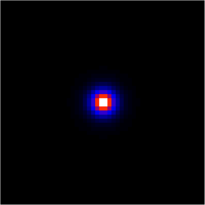
(a) Sextans NFW

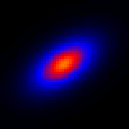
(b) Sextans axisymmetric

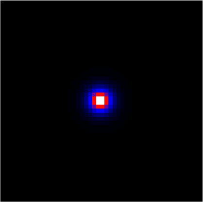
(c) Carina NFW

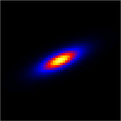
(d) Carina axisymmetric

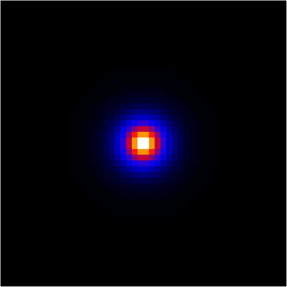
(e) Sculptor NFW

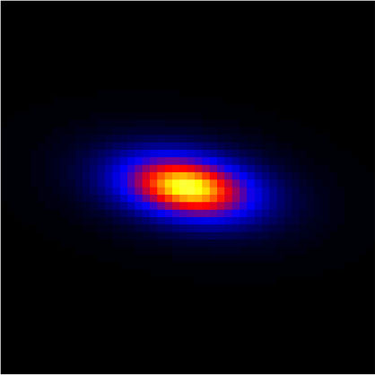
(f) Sculptor axisymmetric

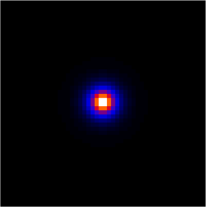
(g) Fornax NFW

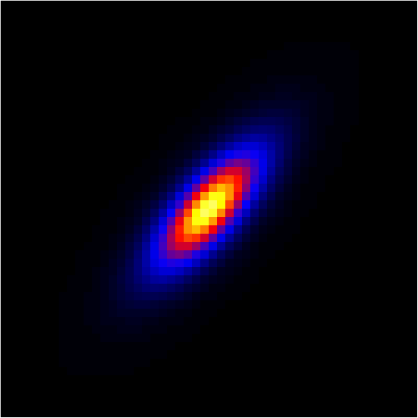
(h) Fornax axisymmetric

Figure 2: DM density profiles projected onto the sky for the dSphs that have a cored halo profile in log scale. From top to bottom, Sextans, Carina, Sculptor and Fornax, where the NFW profiles are shown on the left, and the axisymmetric profiles are shown on the right. The total flux of all images is normalised to unity, and the colour scale is the same in each pair of figures for every dSph. The maps are cropped to correspond to a $5^{\circ}\times 5^{\circ}$ region in the sky.

IV Data Selection and Analysis

We analyse $86$ months (August 4th 2008 15:43:36 till October 15th 2015 02:34:52) of Fermi-LAT PASS8 data in the direction of the selected dSphs using the v10r0p5 version of the Fermi Science Tools. We follow Ref. Ackermann:2015zua for the selection of event class and type (evclass=128, evtype=3) and for the data cuts, which are standard, and use the corresponding instrumental response functions. We analyse a region of interest (ROI) of $10^{\circ}\times 10^{\circ}$ around each dSph, with $0.1^{\circ}$ pixels, and perform a binned likelihood analysis in 24 logarithmically-spaced energy bins from $100$ MeV to $50$ GeV.

We perform the analysis including all the sources included in the third Fermi catalog (3FGL; Acero:2015hja ) within a region with a radius of $25^{\circ}$ around the center of our ROI for each dSph. For the diffuse background, we adopt the latest Galactic diffuse model (gll$\_$iem$\_$v06) and the extragalactic isotropic diffuse model (iso$\_$P8R2$\_$SOURCE$\_$V6$\_$v06) as provided by the Fermi collaboration. We allowed the spectral parameters of the sources to vary within a circle of radius $7.07^{\circ}$—the radius of our ROI—together with the normalisation of the diffuse background components, while the remaining sources are kept fixed to the 3FGL values.

The so-obtained model is complemented in each case with the spatial models of Figs. 1 and 2 for the dSphs’ DM-induced emission. For each dSph, we run two separate analyses with the corresponding NFW and axisymmetric profiles. The spectral part of our dSphs’ models is constructed using Eq. (2) adopting the corresponding J-factor for the NFW or axisymmetric model from Table 1, and making a guess for the value of $\langle\sigma v\rangle$—the parameter that we will constrain. As for the photon spectrum $dN_{f}/dE$, we adopt PYTHIA PYTHIA for the $b\bar{b}$ final state. The normalisation of our dSphs’ models is left free. In each case, we repeat the analysis for 18 values of the DM masses from 10 to 5000 GeV.

We run the binned likelihood analysis following the above prescriptions for each dSph, for both a NFW and an axisymmetric profile, and for each DM mass. When convergence is not achieved, we iterate by filtering out the faintest sources in our model with test statistic (TS) values $\leq 1$, and subsequently $\leq 2$, while making sure that the model is still a good description for the data. We eventually calculate $95$% confidence-level integrated flux upper limits between 100 MeV and 50 GeV for all cases and derive limits on the DM annihilation cross section that we discuss in detail in the next section.

Before we move on to the results, we comment on the model used for the analysis of Sextans. The residual map for Sextans showed the presence of an unmodeled excess at about $3.5^{\circ}$ from the center of the ROI, as shown in Fig. 3, for which we did not find any correspondence in the 3FGL catalog or in the literature. The position of this excess is roughly $(155.93,0.65)$ in celestial coordinates. We fit this excess with a point source described by a simple power law spectrum. We found that this source had a TS value around 1460 and its spectrum was well described by $dN/dE=12.14\times 10^{-9}\left(E/28.04~{}{\rm MeV}\right)^{-2.39}\mathrm{cm^{-2}~{}s^{-1}~{}{MeV}^{-1}}$, with normalisation and spectral index having variations below $1\%$ among the various analyses we ran for the NFW and axisymmetric profiles and different DM masses. In Fig. 3 we show the residual map before and after including this source for one of the analyses. We do not attempt any further modeling or interpretation for this excess, considering our fit just an effective model for it. We are confident that this is a good description of the data for the purposes of our work, also because the derived upper limits on the annihilation cross section from Sextans differ very little if we do or do not model this excess out from the data. Nevertheless, the results that we will discuss in the following section refer to the case where we model this source out.

Note that the Fermi Collaboration published results using energies from 500 MeV to 500 GeV Ackermann:2013yva ; Ackermann:2015zua while we use the 100 MeV to 50 GeV energy range. In particular, Ref. Ackermann:2015zua excluded events below 500 MeV to mitigate the impact of leakage from the bright limb of the Earth. As the same analysis chain is applied to both profile types, the choice of the energy range do not impact the conclusions of our work, i.e., the comparison of the exclusion limits on the DM cross section between NFW and axisymmetric profiles. To confirm this, we perform the analysis of Sextans, which, as will be discussed in the next section, shows the largest difference between the two models, also in the energy range between 500 MeV to 50 GeV. The results are shown in the top right panel of Figure 5. As expected, the limits improve when excluding lower energy events from our analysis, particularly for low DM masses. The limits are consistently better for all tested DM masses in the case of a NFW profile, while in the case of the axisymmetric profile, the limits obtained in the 500 MeV$-$50 GeV range slightly worsen for DM masses above about 100 GeV. At any rate, the relative comparison between the constraints obtained with NFW and axisymmetric profiles is not affected by the choice of the energy range.

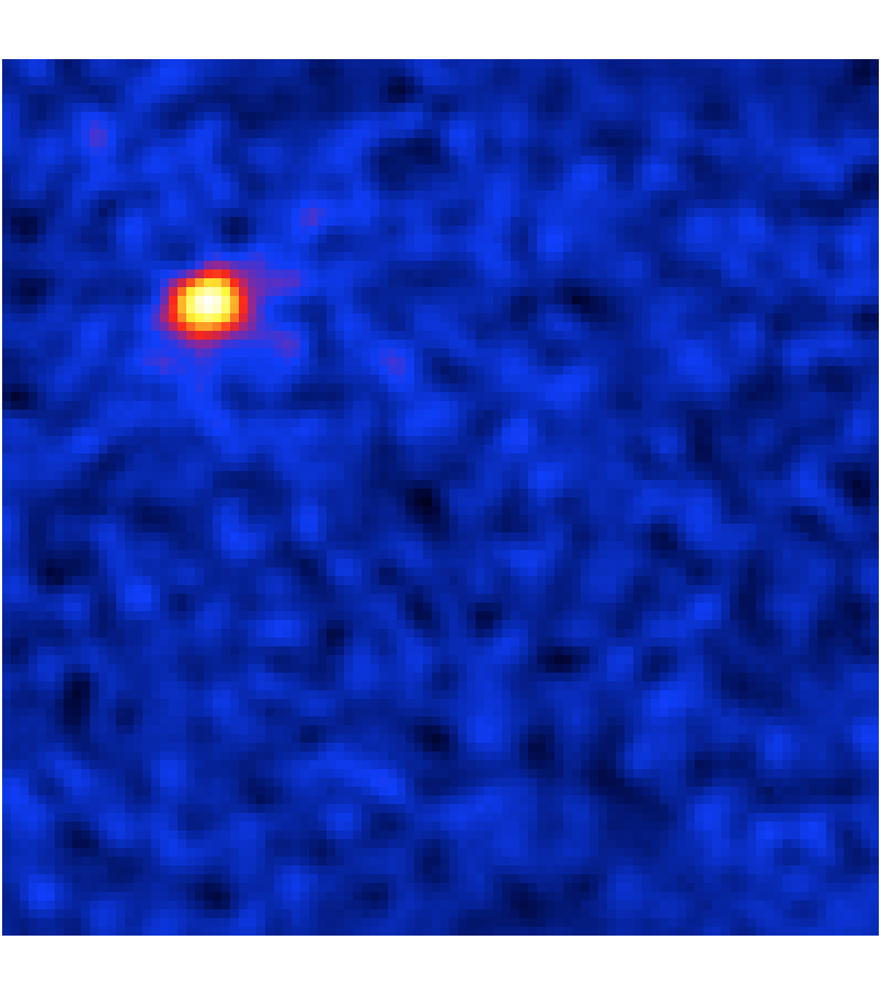
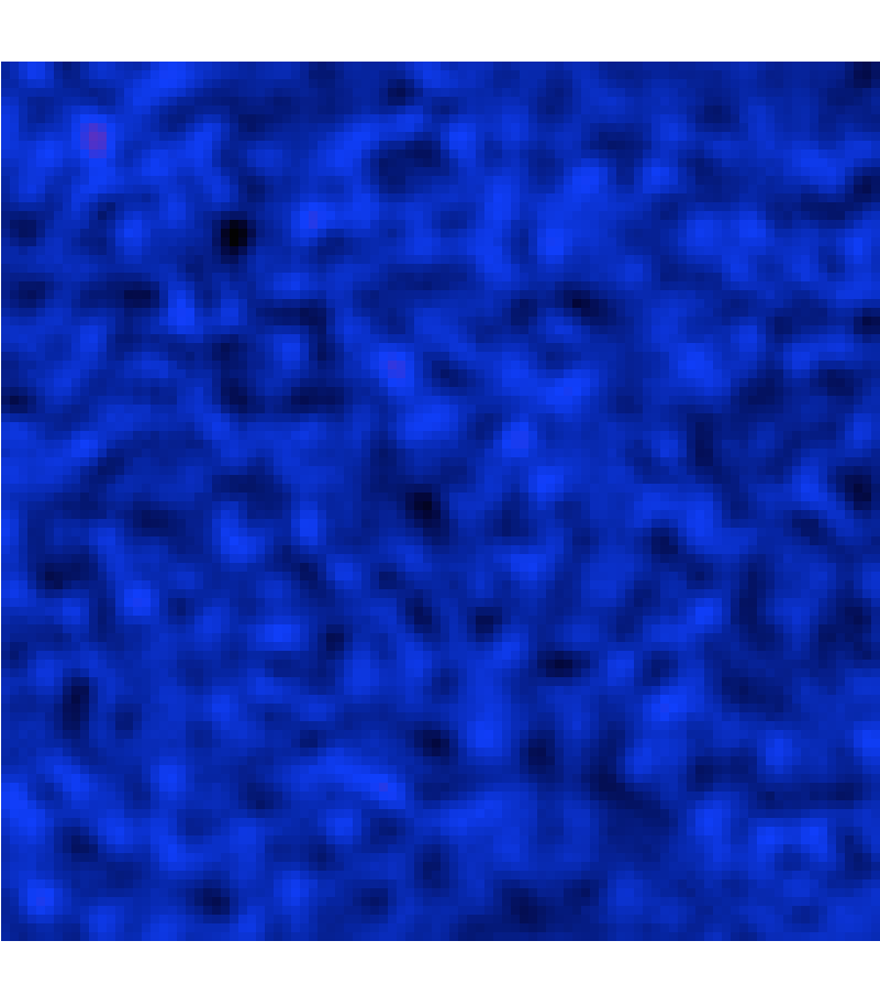
Figure 3: Maps for Sextans, covering $10^{\circ}\times 10^{\circ}$ of the sky. On the left is the residual map before modeling the source, on the right the residual map after modeling the source. The residual maps represent subtractions of the model map from the counts map, therefore the color code refers to residual photon counts.

V Results

We find no gamma-ray excess in any of the dSphs using both the NFW profile and the axisymmetric models. For most of the dSphs and DM masses, we find test statistic (TS) values around zero, and no TS values were larger than $6.06$, which was the case for Fornax using the axisymmetric profile (5.6 using the NFW profile) and a DM mass of $m_{\rm WIMP}=10~{}{\rm GeV}$. Therefore we calculate flux upper limits that we then convert to limits on the annihilation cross section.

We find differences between the cross section upper limits achieved through the two different models of the halo profile. In Figs. 4 and 5, we show the cross section upper limits for the seven analysed dSphs. Figure 4 shows that the dSphs that are expected to have a cusped profile show small differences in the upper limits for the two analysed halo models. Despite the difference in the shape of the two halos (spherical vs oblate), we find that the NFW profile provides a good approximation of the actual halo of these dwarfs.

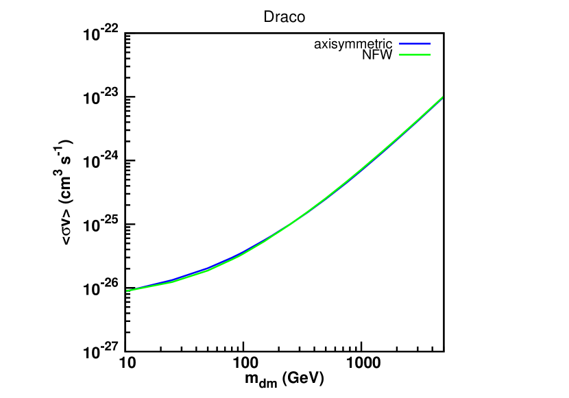
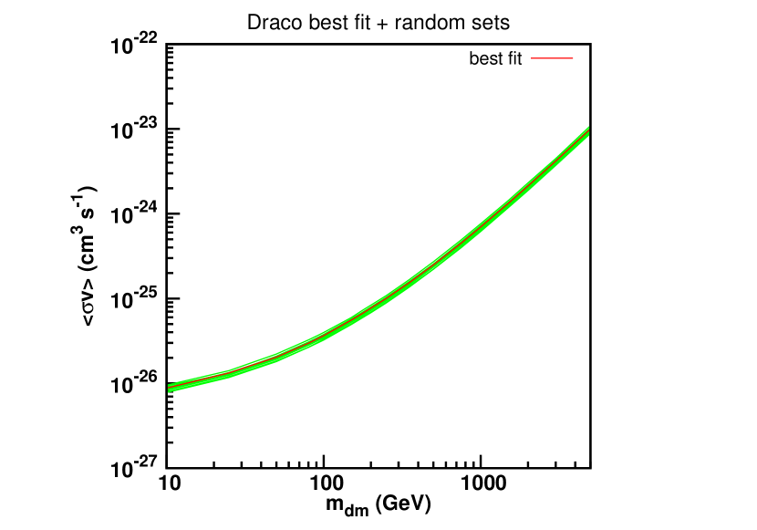
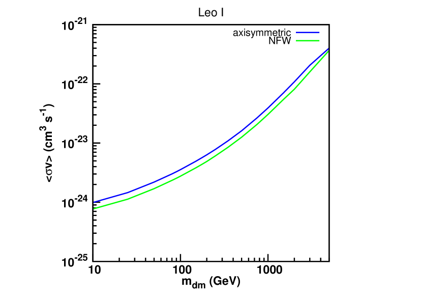
Figure 4: Dark matter annihilation cross section upper limits in the $b\bar{b}$-channel for the dSphs with a cusped profile. The upper right frame shows the cross section upper limits obtained through the analysis of 10 axisymmetric profiles for Draco, corresponding to 10 random sets of the profile parameters from the Monte Carlo sample of Ref. Hayashi:2015yfa , along with the best-fit case.

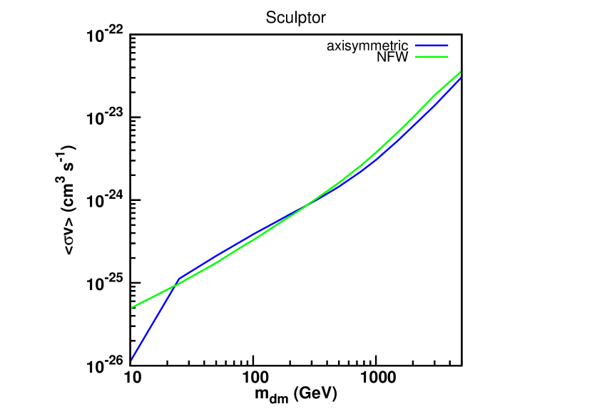
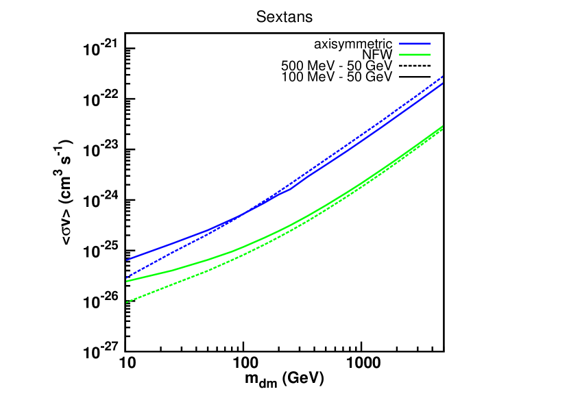
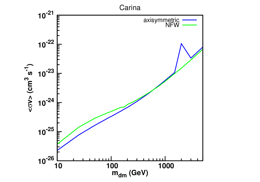
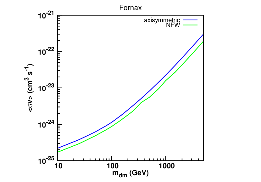
Figure 5: Dark matter annihilation cross section upper limits in the $b\bar{b}$-channel for the dSphs with a cored profile.

The impact of the different profiles is more significant for the four dSphs that have a cored profile as suggested by the observationally motivated profile we adopted and shown in Fig. 5. In particular, we find the largest difference of about a factor of 2.5–7, depending on the DM-particle mass, in the case of Sextans, where we see that the axisymmetric model is most extended compared with the corresponding NFW profile as shown in Fig. 2. The upper right panel in Fig. 5 shows the resulting cross section upper limits of Sextans derived both in the energy range 100 MeV$-$50 GeV and 500 MeV$-$50 GeV. As anticipated in the previous section, the difference between the NFW and axisymmetric profiles is unaffected by this choice. It is, in fact, even slightly larger – a factor of 3–11 depending on the DM-particle mass – for the 500 MeV$-$50 GeV energy range. Therefore, given that Sextans was one of the most important dSphs with the spherically symmetric model, i.e., cross section upper limits reached the canonical value $3\times 10^{-26}~{}\mathrm{cm^{3}~{}s^{-1}}$ for low-mass WIMPs, we show that it is indeed relevant to use a more accurate model for its density profile.

The most stringent constraints on $\langle\sigma v\rangle$ are obtained for Draco, whose $J$-factor is the largest among the seven dSphs analyzed here. In this case, the canonical annihilation cross section $\langle\sigma v\rangle=3\times 10^{-26}~{}\mathrm{cm^{3}~{}s^{-1}}$ can be tested for WIMPs lighter than $\sim$80 GeV, and since the DM density is described by the cusped profile, there is only little difference between the spherical and axisymmetric models. Although the results of the combined likelihood analysis (e.g., Ref. Ackermann:2015zua ) will be dominated by the most promising dSphs such as Draco, others, such as Sextans discussed above, will also give a substantial contribution. Therefore, the inclusion of observationally-motivated axisymmetric profiles would make the joint likelihood analysis of the dSphs slightly weaker compared to the previous analysis in the literature.

To test the impact of measurement uncertainties of stellar kinematics data on these gamma-ray constraints, we randomly choose ten sets of the parameters from the Monte Carlo sample of Ref. Hayashi:2015yfa for the Draco axisymmetric profile, and obtain the cross section upper limits for each, whose results are shown in the upper right panel of Fig. 4 along with the best-fit case. This shows that the current stellar kinematics data are well determined, giving only uncertainties on the cross section upper limits of about 10%, which makes dSphs a robust, and hence, attractive object to test DM annihilation. This also shows that our comparison between NFW and axisymmetric profiles is not significantly affected by the uncertainties on the latter and that our conclusions are robust.

We note that a kink around $\sim$2 TeV for the axisymmetric model of Carina as well as a drop toward $\sim$10 GeV of Sculptor is likely caused by some complicated interplay between the adopted profile, energy spectrum, and photon count distribution that we interpret as a statistical fluctuation, also considering that the models for these particular cases of $m_{\mathrm{dm}}$ show no substantial difference, i.e., in TS significance, with respect to the others.

Finally, we note that although evaluating the integrated $J$-factor will capture the overall importance of each dSph, it is not until one performs the likelihood analysis that we know how the cross section upper limits behave as a function of the WIMP mass. In fact, the difference in the cross section upper limits comes from an interplay of the normalisation and shape of the $J$-factor. For example, the difference between the $J$-factors is larger for Leo I than for Fornax, with a value of 0.78 against 0.91 for the ratio $J_{\text{axisymmetric}}/J_{\mathrm{NFW}}$. The difference between the upper limits however is larger for Fornax, where the upper limit for the axisymmetric case is up to 1.57 times larger than the NFW case, while up to 1.33 times larger in the case of Leo I. So the difference between the shapes of the halo models has a larger contribution to the difference in the cross section upper limits than the difference between the total $J$-factors. While Ref. Bonnivard:2014kza studied $J$-factors for a comprehensive list of dSphs, our focus is on the classical seven dSphs that have the best measurements of stellar kinematics, and we performed the likelihood analysis for all of them. Therefore, these two approaches are complementary to each other.

Before moving to the conclusions, we want to underline that the cross section upper limits shown here, differently from Refs. Ackermann:2013yva ; Ackermann:2015zua , are obtained without taking in consideration any uncertainty, i.e., without marginalising over the uncertainty on, e.g., the J-factor determination. However, this has no impact on the relative comparison that we set out to make between the NFW and axisymmetric profiles.

VI Conclusion

Dwarf spheroidal galaxies are important and well established targets for indirect DM searches. The most common choice for the DM density profile in the analysis of these dSphs is an NFW profile. Recent observational data of stellar kinematics, however, imply that DM halos around these galaxies are better described by an axisymmetric profile, with an axis ratio of 0.6–0.8, either cored or cusped. For this reason, we investigated the impact of adopting observationally-motivated axisymmetric models instead of the commonly adopted NFW profile on the limits obtained for the DM annihilation cross section for seven classical dSphs with Fermi gamma-ray data.

Draco is the most promising dwarf galaxy among the seven analysed. Although its DM distribution is well described by a cusped oblate profile in the axisymmetric modeling, the total amount of gamma rays yielding from the overall region will be similar to that of an NFW profile (i.e., similar $J$-factors). As a result, we obtained very similar upper limits on the annihilation cross section for Draco using an NFW and axisymmetric model. The same is true for Leo II, while Leo I shows some mild differences, even if both feature an inner cusp. By testing ten axisymmetric profiles randomly chosen from a Monte Carlo sample of the analyses of stellar kinematics data of Draco, we find that the current uncertainty on the density profile of Draco will give a systematic uncertainty on the cross section upper limits of about 10%. This proves that our conclusions are robust.

The analyses of the dSphs best described by a cored profile (Sextans, Sculptor, Carina and Fornax) result in a more substantial difference between the two adopted profiles. In particular, for Sextans, the best-fit model of its stellar kinematics data yields a much more extended $J$-factor map. We found that the cross section upper limits were weaker by a factor of a few to several compared with those obtained with an NFW profile. This demonstrates the importance of properly assessing DM density profiles from observational data, and also that upper limits in the literature obtained assuming a cusped spherical model (such as an NFW) might be overestimated.

- (1) E. Komatsu et al., ApJS 192, 18 (2011), 1001.4538.
- (2) Planck, P. A. R. Ade et al., Astron. Astrophys. 594, A13 (2016), 1502.01589.
- (3) G. Bertone, D. Hooper, and J. Silk, Physics Reports 405, 279 (2005), hep-ph/0404175.
- (4) J. M. Gaskins, Contemp. Phys. 57, 496 (2016), 1604.00014.
- (5) E. Aliu et al., ApJ 697, 1299 (2009), 0810.3561.
- (6) V. A. Acciari et al., ApJ 720, 1174 (2010), 1006.5955.
- (7) J. Aleksić et al., JCAP 6, 035 (2011), 1103.0477.
- (8) M. Ackermann et al., Physical Review Letters 107, 241302 (2011), 1108.3546.
- (9) E. Aliu et al., Physics Review D 85, 062001 (2012), 1202.2144.
- (10) J. Aleksić et al., JCAP 2, 008 (2014), 1312.1535.
- (11) A. A. Abdo et al., ApJ 712, 147 (2010), 1001.4531.
- (12) M. Ackermann et al., Physics Review D 89, 042001 (2014), 1310.0828.
- (13) A. Abramowski et al., Physics Review D 90, 112012 (2014), 1410.2589.
- (14) A. Geringer-Sameth, S. M. Koushiappas, and M. G. Walker, Phys. Rev. D91, 083535 (2015), 1410.2242.
- (15) M. Ackermann et al., Physical Review Letters 115, 231301 (2015), 1503.02641.
- (16) A. Geringer-Sameth et al., Phys. Rev. Lett. 115, 081101 (2015), 1503.02320.
- (17) A. Drlica-Wagner et al., ApJl 809, L4 (2015), 1503.02632.
- (18) MAGIC Collaboration, JCAP 2, 039 (2016), 1601.06590.
- (19) S. Li et al., Phys. Rev. D 93, 043518 (2016).
- (20) A. Abramowski et al., Physical Review Letters 106, 161301 (2011), 1103.3266.
- (21) D. Hooper and T. Linden, Physics Review D 84, 123005 (2011), 1110.0006.
- (22) A. Abramowski et al., Physical Review Letters 114, 081301 (2015), 1502.03244.
- (23) F. Calore, I. Cholis, and C. Weniger, JCAP 3, 038 (2015), 1409.0042.
- (24) T. Daylan et al., Physics of the Dark Universe 12, 1 (2016), 1402.6703.
- (25) F. Calore, I. Cholis, C. McCabe, and C. Weniger, Physics Review D 91, 063003 (2015), 1411.4647.
- (26) M. Ajello et al., ApJ 819, 44 (2016).
- (27) B. Zhou et al., Phys. Rev. D91, 123010 (2015), 1406.6948.
- (28) J. Aleksić et al., ApJ 710, 634 (2010), 0909.3267.
- (29) M. Ackermann et al., JCAP 5, 025 (2010), 1002.2239.
- (30) A. Abramowski et al., ApJ 750, 123 (2012), 1202.5494.
- (31) S. Ando and D. Nagai, JCAP 7, 017 (2012), 1201.0753.
- (32) T. Arlen et al., ApJ 757, 123 (2012), 1208.0676.
- (33) M. Ackermann et al., ApJ 812, 159 (2015), 1510.00004.
- (34) B. Anderson et al., JCAP 2, 026 (2016), 1511.00014.
- (35) Y.-F. Liang et al., Phys. Rev. D 93, 103525 (2016).
- (36) M. Ackermann et al., Physics Review D 85, 083007 (2012), 1202.2856.
- (37) M. Fornasa et al., MNRAS 429, 1529 (2013), 1207.0502.
- (38) S. Ando and E. Komatsu, Physics Review D 87, 123539 (2013), 1301.5901.
- (39) S. Ando, A. Benoit-Lévy, and E. Komatsu, Physics Review D 90, 023514 (2014), 1312.4403.
- (40) G. A. Gómez-Vargas et al., Nuclear Instruments and Methods in Physics Research A 742, 149 (2014), 1303.2154.
- (41) M. Fornasa and M. A. Sánchez-Conde, Physics Reports 598, 1 (2015), 1502.02866.
- (42) A. Cuoco et al., ApJs 221, 29 (2015), 1506.01030.
- (43) S. Camera, M. Fornasa, N. Fornengo, and M. Regis, JCAP 6, 029 (2015), 1411.4651.
- (44) N. Fornengo, L. Perotto, M. Regis, and S. Camera, ApJl 802, L1 (2015), 1410.4997.
- (45) M. Regis et al., Phys. Rev. Lett. 114, 241301 (2015), 1503.05922.
- (46) S. Ando and K. Ishiwata, JCAP 1606, 045 (2016), 1604.02263.
- (47) M. Fornasa et al., (2016), 1608.07289.
- (48) M. L. Mateo, Annual Review of Astronomy and Astrophysics 36, 435 (1998), astro-ph/9810070.
- (49) L. E. Strigari, S. M. Koushiappas, J. S. Bullock, and M. Kaplinghat, Physics Review D 75, 083526 (2007), astro-ph/0611925.
- (50) L. E. Strigari et al., ApJ 678, 614 (2008), 0709.1510.
- (51) M. A. Sánchez-Conde, M. Cannoni, F. Zandanel, M. E. Gómez, and F. Prada, JCAP 12, 011 (2011), 1104.3530.
- (52) A. Chiappo et al., (2016), 1608.07111.
- (53) J. F. Navarro, C. S. Frenk, and S. D. M. White, Astrophys. J. 490, 493 (1997), astro-ph/9611107.
- (54) J. Einasto, Trudy Astrofizicheskogo Instituta Alma-Ata 5, 87 (1965).
- (55) A. W. McConnachie, Astronomical Journal 144, 4 (2012), 1204.1562.
- (56) C. A. Vera-Ciro, L. V. Sales, A. Helmi, and J. F. Navarro, MNRAS 439, 2863 (2014), 1402.0903.
- (57) P. Ullio and M. Valli, JCAP 1607, 025 (2016), 1603.07721.
- (58) V. Bonnivard, C. Combet, D. Maurin, and M. G. Walker, Mon. Not. Roy. Astron. Soc. 446, 3002 (2015), 1407.7822.
- (59) K. Hayashi and M. Chiba, Astrophys. J. 810, 22 (2015), 1507.07620.
- (60) G. D. Martinez, mnras 451, 2524 (2015), 1309.2641.
- (61) J. Binney and S. Tremaine, Galactic dynamics (, 1987).
- (62) S. Colafrancesco, S. Profumo, and P. Ullio, Phys. Rev. D75, 023513 (2007), astro-ph/0607073.
- (63) K. Hayashi et al., Mon. Not. Roy. Astron. Soc. 461, 2914 (2016), 1603.08046.
- (64) J. Binney and S. Tremaine, Galactic Dynamics: Second Edition (Princeton University Press, 2008).
- (65) M. Cappellari, mnras 390, 71 (2008), 0806.0042.
- (66) E. Tempel and P. Tenjes, mnras 371, 1269 (2006), astro-ph/0606680.
- (67) H. C. Plummer, mnras 71, 460 (1911).
- (68) Fermi-LAT, F. Acero et al., Astrophys. J. Suppl. 218, 23 (2015), 1501.02003.
- (69) T. Sjostrand, S. Mrenna, and P. Z. Skands, JHEP 05, 026 (2006), hep-ph/0603175.