A New Architecture for
Optimization Modeling Frameworks
Abstract
We propose a new architecture for optimization modeling frameworks in which solvers are expressed as computation graphs in a framework like TensorFlow rather than as standalone programs built on a low-level linear algebra interface. Our new architecture makes it easy for modeling frameworks to support high performance computational platforms like GPUs and distributed clusters, as well as to generate solvers specialized to individual problems. Our approach is particularly well adapted to first-order and indirect optimization algorithms. We introduce cvxflow, an open-source convex optimization modeling framework in Python based on the ideas in this paper, and show that it outperforms the state of the art.
I Introduction
Optimization offers a principled approach to solving problems in a wide variety of application domains, such as machine learning, statistics, control, signal and image processing, networking, engineering design, finance, and many others [BV04]. Instead of designing specialized algorithms for each individual problem, the user describes the problem as the minimization of a cost function and the optimal solution with minimal cost is found by the optimization method.
The wealth of applications for this methodology has driven the development of several high-level modeling languages. These languages provide a separation of concerns between the development of mathematical models and the implementation of numerical routines to optimize these models. This is especially useful for rapidly prototyping new applications, allowing practitioners to easily experiment with different cost functions and constraints by writing expressions that closely mimic the mathematical optimization problem. Prominent examples of modeling languages and frameworks include AMPL [FGK02], YALMIP [Lof04], and CVX [GB14], as well as several tied closely to particular solvers, such as CPLEX’s ILOG [ILO07] and MathProg from GLPK [Mak00].
Despite the popularity of these modeling frameworks, support for modern large-scale computational environments such as GPUs and distributed clusters is virtually nonexistent. In part, this is due to fundamental challenges in scaling interior point methods, which have historically been the basis for solvers of most modeling frameworks, as these methods require solving sparse linear systems to high accuracy and as such do not benefit greatly from GPU implementation. In addition, distributing such methods beyond a single machine typically requires high bandwidth interconnects such as those available exclusively in HPC environments.
However, there are also highly practical reasons for the lack of support for new environments: mature solvers often require several years to develop and writing entirely new implementations of low-level numerical routines specialized to each environment is unappealing. Traditionally, a degree of platform independence has been provided by implementing on top of low-level linear algebra libraries (e.g., BLAS, LAPACK, and SuiteSparse), but as we discuss in this paper, this architecture is often insufficient, especially for large problems. In addition, such libraries do not handle memory management and data transfer between GPU and CPU or between multiple machines.
The solution that we explore is a new architecture for optimization modeling frameworks based on solvers represented as computation graphs. This architecture is well-suited for solving large optimization problems by taking advantage of problem-specific structure. In particular, the computation graph abstraction naturally represents the composition of structured linear operators which can be significantly more efficient than the standard sparse or dense matrix representation. We develop such a method in this paper and demonstrate that it outperforms the existing state of the art for solving large convex optimization problems, a GPU-enabled version of SCS [OCPB16], which itself is one of the few GPU-optimized solvers available, POGS [FB15] being another example.
A secondary, but not insignificant, benefit of this approach is automatic support for a wide variety of computational environments (CPU, GPU, distributed clusters, etc.), leveraging the considerable momentum and engineering effort of existing computation graph frameworks from the deep learning community. A potential drawback of our approach is that the runtime system must support the necessary mathematical operations to implement numerical optimization algorithms. For first-order and indirect solvers, the many frameworks developed for deep learning, such as TensorFlow [AAB+16], Theano [BBB+10, BLP+12], Caffe [JSD+14], and Torch [CKF11], provide all the necessary functionality. The frameworks have only limited support, however, for the sparse matrix factorization routines used by direct solvers. Thus, given the computation graph implementations available at this time, our architecture tends to favor first-order and indirect methods as opposed to interior point methods.
The outline of the paper is as follows. In §II, we review the traditional architecture for optimization modeling frameworks and discuss its shortcomings. In §III, we explore prior work that addressed the shortcomings of the traditional architecture. In §IV, we describe the new architecture we propose and the computation graph abstraction the architecture is based on. In §V, we present cvxflow, an open-source implementation of the ideas in this paper, and numerical results comparing cvxflow with the state of the art.
II Traditional architecture
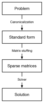
The traditional architecture for optimization modeling frameworks dates back to AMPL [FGK02] and GAMS [BKMR88] in the 1980s. In this architecture, solving an optimization problem is divided into a three step process, shown in Fig. 1. The process begins with a high-level description of the optimization problem expressed in a modeling language. The first step is canonicalization, in which the problem is transformed through symbolic manipulation into an equivalent problem in a standard form. The second step is matrix stuffing, in which the symbolic representation of the standard form is instantiated so that linear operators are represented by sparse matrices. Often canonicalization and matrix stuffing are combined into a single step. The final step is to call a solver with the sparse matrix representation of the standard form as input and return the solver output as the solution.
The ecosystem of modeling frameworks for convex optimization is an illustrative example of the traditional architecture. Convex optimization modeling languages are built around the principles of disciplined convex programming, a set of rules for constructing optimization problems that make it easy to verify problem convexity. Implementations include CVX [GB14] and YALMIP [Lof04] in MATLAB, CVXPY [DB16a] in Python, Convex.jl [UMZ+14] in Julia, and the standalone compilers CVXGEN [MB12] and QCML [CPDB13]. We discuss each component of the traditional architecture in the concrete case of convex modeling frameworks.
II-A Canonicalization
The standard form for convex optimization problems is a cone program, an optimization problem of the form
| (1) |
where is the optimization variable; , , and are constants; and is a nonempty closed convex cone [NN92]. Convex optimization modeling frameworks symbolically convert problems into cone programs via epigraph transformations [GB08].
II-B Matrix stuffing
In solvers and other software that use the cone program standard form as an input format for problems, and are represented by arrays and is represented by a standard sparse matrix format, such as column compressed storage. Matrix stuffing generates a sparse matrix representation of from the symbolic representation generated through canonicalization [DB16b]. Solvers use a sparse matrix representation of because they generally use algorithms and libraries that exploit sparsity.
II-C Solver
A wide variety of solver implementations have been developed for problems in the cone program standard form. Many solvers are written in pure C, including MOSEK [Mos15], SDPA [YFF+12], ECOS [DCB13], and SCS [OCPB16]. Other solvers are written in higher level languages, such as SeDuMi [Stu99] and SDPT3 [TTT99] in MATLAB and CVXOPT [ADV15] in Python. The solvers rely heavily on low-level linear algebra interfaces like BLAS and LAPACK [LHKK79] for basic operations and libraries like SuiteSparse [Dav16] for sparse matrix factorization. Existing cone solvers are almost exclusively restricted to CPU implementations; an exception is SCS which provides GPU support using the cuBLAS library [NVI08].
II-D Drawbacks
The traditional approach to optimization modeling frameworks has been enormously successful, allowing modeling languages and solver implementations to be developed independently in the programming languages best suited to their function. The conventional solver implementation is based on interior point methods, for which the dominant computational effort is solving a sparse linear system. Such a solver can be ported relatively easily to new platforms provided the necessary linear algebra libraries (BLAS, LAPACK, SuiteSparse, etc.) are available.
However, many optimization problems of interest are too large to be solved with interior point methods and, more generally, any method that requires a direct solution to a linear system involving the matrix of the cone program standard form (1). In some problem domains the memory requirements even for sparse matrices can be prohibitive (e.g., 2D convolution in large-scale image reconstruction), while at the same time efficient procedural evaluations of the matrix-vector computations with and exist (e.g., FFT-based convolution).
A possible solution is a first-order method, such as SCS [OCPB16], which only requires solving linear systems to moderate accuracy. This approach can be implemented with either a direct or indirect method for the linear solver subroutine. In the case of a direct solver, the computational cost can be amortized by caching the factorization of the matrix leading to iterations that are significantly faster than interior point methods. In the indirect case, a matrix-free method such as conjugate gradient is used, requiring only matrix-vector computations with and . In the traditional architecture, these computations are simply implemented with sparse matrix multiplies, but the proposed graph-based approach enables taking advantage of specialized linear operator implementations, as we will discuss in detail in the next section.
III Alternative approaches
Prior work has explored alternative approaches to bypassing the limitations of the traditional architecture for optimization modeling frameworks, with a focus on scaling to larger problem sizes. There are two main lines of work that are precursors to the graph-based architecture proposed in this paper: the first replaces the sparse matrix representation of the standard form generated by matrix stuffing with a more general representation, and the second explores new standard forms based on functions with efficient proximal operators. In this section, we review these approaches, providing motivation for our general graph-based framework.
III-A Abstract linear operators
In solving many convex optimization problems, the majority of computational time is spent in evaluating linear operators. While the sparse matrix representation of cone programs is fully general, it does not provide the most efficient implementation for many types of linear functions. Matrix-free CVXPY replaces traditional sparse matrix representation of the cone program standard form (1) with a computation graph based representation. The computation graph representation allows the modeling layer to encode information about structured linear operators in the optimization problem that solvers can exploit [DB16b]. The matrix-free CVXPY implementation includes a custom runtime system for computation graphs, as opposed to the cvxflow implementation presented in this paper, which is built on TensorFlow.
III-B Proximal standard forms
Another line of work explores solvers based on functions with efficient proximal operators. Epsilon [WWK15] introduces the standard form
| (2) |
where is the optimization variable, are linear operators, and are functions with efficient proximal operators [PB14]. Epsilon exploits the flexibility of the standard form (2) to rewrite the problem so it can be solved efficiently by a variant of the alternating direction method of multipliers (ADMM) [BPC+11]. Along similar lines, POGS [FB15] introduces a slightly different standard form, again based on functions with efficient proximal operators, and includes a highly efficient GPU implementation of an ADMM-based algorithm.
The ProxImaL modeling framework also targets the standard form (2), but supports a variety of solver algorithms and applies problem rewritings specialized to optimization problems in imaging [HDN+16]. ProxImaL moves towards platform independence by generating solver implementations using Halide [RKBA+13]. Halide is a language and compiler that allows for platform independent abstraction of individual mathematical operations, but not of full algorithms composed of many operations inside control logic.
These new proximal standard forms are not necessarily incompatible with the traditional architecture based on sparse matrices. However, as opposed to cone solvers and in particular interior point methods, the implementation of algorithms operating on the proximal standard forms is less reliant on sparse linear algebra and thus there is less benefit from building on existing sparse linear algebra libraries. These approaches instead require a library of proximal operator implementations which can benefit greatly from being built on a high-level framework such as Halide or TensorFlow, providing platform independence and a highly optimized runtime system.
IV Graph-based architecture
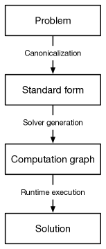
In this section, we propose a new graph-based architecture for optimization modeling frameworks. Our architecture divides the process of solving an optimization problem into three steps, shown in Fig. 2. As with the traditional architecture we begin with a high-level problem description which is canonicalized to a standard form. The solver generation step produces a computation graph representing the solver algorithm, which is executed by the runtime system to produce a solution.
The key difference from the traditional architecture is that the graph-based approach directly generates computation graphs representing the numerical algorithms for solving problems rather than representing all problems with sparse matrices. The first benefit of this approach is support for abstract linear operators with highly efficient implementations, such as convolution, Kronecker products, and others. The second benefit is a closer connection between canonicalization and solver generation, which can now both be implemented in the same high-level language and even in a single library. This more easily allows for supporting different standard forms that incorporate problem-specific structure. Finally, the new architecture severs the link between the solver implementation and computing platform, allowing solvers to take advantage of new computing platforms simply by changing the target of the computation graph runtime system.
We next explain the central abstraction, computation graphs, and describe how such graphs representing solvers are generated.
IV-A Computation graphs
A computation graph is a directed acyclic graph (DAG) where each vertex represents a mathematical operation and each edge represents data transfer. Input vertices have no incoming edges, while output vertices have no outgoing edges. A vertex is evaluated by applying its operation to the data on the vertex and broadcasting the result on its outgoing edges. The overall graph is evaluated by loading data onto the input vertices, evaluating the vertices in topological order, and reading the results off the output vertices.
For example, Fig. 3 shows a computation graph for the function . The input vertices represent the variables and . The output vertex represent the top level sum. The internal vertices represent the operations and .
Given a computation graph to evaluate a function, computation graphs for evaluating the function’s gradient or adjoint (for linear functions) can be obtained through simple graph transformations [Gri89, DB16b]. Function, gradient, and adjoint evaluations are the key operations in first-order and indirect solvers and are even sufficient to precondition a problem [DB16c].
Computation graphs are a useful intermediate representation for solvers because they abstract away the platform-specific details of both computation and memory management. These details are handled by a computation graph runtime system, which has platform-specific code to execute each mathematical operation and to pass data from one operation to the next. By contrast, a solver built on the traditional abstraction of a low-level linear algebra interface must implement its own platform-specific logic for mathematical operations not expressible as linear functions and for memory management.
IV-B Solver generation
The solver generation step produces a computation graph representing a numerical algorithm for solving an optimization problem. Graph generation is naturally implemented in a high-level functional programming style with modular functions that produce computation graphs implementing numerical algorithms or subroutines. Typically, these functions take as inputs individual nodes or in some cases are naturally parameterized by graph generator functions.
As a concrete example, the Python code snippet for generating a TensorFlow graph representing the conjugate gradient method for the linear system is shown below.
def cg_solve(A, b, x_init, tol=1e-8):
  delta = tol*norm(b)

  def body(x, k, r_norm_sq, r, p):
    Ap = A(p)
    alpha = r_norm_sq / dot(p, Ap)
    x = x + alpha*p
    r = r - alpha*Ap
    r_norm_sq_prev = r_norm_sq
    r_norm_sq = dot(r,r)
    beta = r_norm_sq / r_norm_sq_prev
    p = r + beta*p
    return (x, k+1, r_norm_sq, r, p)

  def cond(x, k, r_norm_sq, r, p):
    return tf.sqrt(r_norm_sq) > delta

  r = b - A(x_init)
  loop_vars = (
      x_init, tf.constant(0),
      dot(r, r), r, r)
  return tf.while_loop(
      cond, body, loop_vars)[:3]
In this example, the function cg_solve is parameterized by the the linear operator A, and vector b with initial starting point, vector x_init. The inputs b and x_init are computation graph nodes and A is a single-argument function such that A(x) produces the computation graph representing the linear operator applied to an arbitrary vector x. Implemented in this fashion, the conjugate gradient method can be applied to any linear operator expressed as a computation graph.
V Numerical examples
In this section, we present numerical examples of solving convex optimization problems in our proposed architecture. As solving linear systems forms the basis for convex methods, we first present results for an indirect linear solver with various linear operators. Using this indirect linear solver as a subroutine, we then implement a version of SCS [OCPB16] in the computation graph framework and compare with the native version of SCS implemented in C. We present results for both CPU and GPU environments; all experiments are run on a 32-core Intel Xeon 2.2GHz processor and an nVidia Titan X GPU with 12GB of RAM.
Our implementation builds on CVXPY [DB16a], a convex optimization modeling framework in Python. Using this framework, convex optimization problems can be expressed with minimal code and are automatically converted into the standard conic form (1). As an example, the nonnegative deconvolution problem we consider in Section V-C is written as the following Python code.
from cvxpy import *
x = Variable(n)
f = norm(conv(c, x) - b, 2)
prob = Problem(Minimize(f), [x >= 0])
Here c and b are previously-defined problem inputs and n is the size of the optimization variable. Our implementation differs from the existing CVXPY functionality in that instead of solving problems by constructing sparse matrices and calling numerical routines written in C, we build a computation graph, as described in Section IV, and evaluate with TensorFlow. Ultimately, this implementation achieves faster running times than existing methods—for example, on the large nonnegative deconvolution example, our implementation takes roughly 1/10th the time of SCS running on GPU, the existing state-of-the-art method for solving large convex problems to moderate accuracy.
Concurrent with the publication of this paper, we are releasing the cvxflow Python library; it is available at
and includes the code for all of the examples in this section. The implementation is general and solves any problem modeled with CVXPY using TensorFlow.
V-A Regularized least squares
We begin with solving linear systems using the conjugate gradient method (CG) [HS52]. CG is matrix-free which makes it a natural fit for linear systems represented as a graph, allowing for specialized implementations of each linear operator including those that are inefficient to represent as sparse matrices such as convolution, Kronecker products, and others. In terms of the graph-based architecture shown in Fig. 2, the standard form in this example is a linear system and the solver generation step generates a graph representing the conjugate gradient method.
In particular, we consider the regularized least squares problem
| (3) |
where is the optimization variable, the linear map and vector are problem data, and is the regularization parameter. This problem has the solution
| (4) |
which can be computed by solving a linear system.
It is often the case that takes the form of a sparse or dense matrix; for example, in a statistical problem each row of may represent an observation of multiple variables weighted by in order to predict the response variable. However, can also be an abstract linear operator; for example, a convolution with a vector , written as . We present results for each of these examples: a sparse matrix, a dense matrix, and convolution.
In the matrix examples, entries are sampled from with 1% nonzero in the sparse case. For convolution, we apply the Gaussian kernel with standard deviation . In all cases, the response variable is formed by where has entries sampled from and from . The conjugate gradient method is run until the residual satisfies .
| dense matrix | sparse matrix | convolution | |
| variables | 3000 | 3000 | 3000 |
| nonzeros in | 18000000 | 180000 | 4095000 |
| spsolve | |||
| solve time | 255 secs | 28 secs | 41 secs |
| memory usage | 2.2 GB | 1.06 GB | 1.5 GB |
| objective | |||
| CG TensorFlow | |||
| solve time, CPU | 3.0 secs | 0.9 secs | 2.9 secs |
| solve time, GPU | 2.0 secs | 0.7 secs | 1.0 secs |
| graph build time | 0.4 secs | 0.1 secs | 0.1 secs |
| memory usage | 1.8 GB | 755 MB | 946 MB |
| objective | |||
| CG iterations | 49 | 49 | 71 |
Table I shows the results for these experiments, demonstrating that conjugate gradient on TensorFlow is significantly faster than the baseline method, scipy.sparse.spsolve. This is a somewhat weak baseline as spsolve does not run on GPU and is not well-suited for dense matrices. Nonetheless, this comparison highlights the difference in architecture exploited by TensorFlow which can take advantage of dedicated implementations for the linear operators leading to significantly faster solve times.
V-B Lasso
| dense matrix | sparse matrix | convolution | |
| variables | 6001 | 6001 | 6001 |
| constraints | 12002 | 12002 | 12001 |
| nonzeros in | 18012002 | 1812002 | 4107002 |
| SCS native | |||
| solve time, CPU | 29 secs | 3.4 secs | 6.4 secs |
| solve time, GPU | 27 secs | 3.8 secs | 7.6 secs |
| matrix build time | 13 secs | 1.4 secs | 2.8 secs |
| memory usage | 3.1 GB | 663 MB | 927 MB |
| objective | |||
| SCS iterations | 40 | 40 | 60 |
| avg. CG iterations | 2.66 | 2.71 | 2.72 |
| SCS TensorFlow | |||
| solve time, CPU | 23 secs | 25 secs | 24 secs |
| solve time, GPU | 9.9 secs | 7.1 secs | 5.3 secs |
| graph build time | 1.8 secs | 2.0 secs | 0.8 secs |
| memory usage | 8.7 GB | 4.6 GB | 1.2 GB |
| objective | |||
| SCS iterations | 60 | 40 | 180 |
| avg. CG iterations | 3.35 | 3.55 | 1.93 |
Next we solve a convex problem with SCS [OCPB16]. In this case, the canonicalization step produces a problem in the standard cone form (1) and solver generation produces a graph implementing the SCS iterations. In essence, the algorithm iterates between projections onto a linear subspace and a convex cone; the former is done through solving a linear system with a computation graph representing the CG method as in the previous section. The SCS method is appealing in this context as it works well with approximate solutions to linear systems, such as those produced by CG.
We consider the lasso problem
| (5) |
where the regularization term replaces the in the regularized least squares problem from the previous section. This problem is convex but no longer has a closed-form solution.
To generate problem instances, we construct example linear operators as in the previous section. We set the regularization parameter to where is the smallest value of such that the solution is zero.
Table II compares the TensorFlow version of SCS to the native implementation and demonstrates that in the dense matrix and convolution cases, the solve time on GPU is faster with TensorFlow. This highlights the benefit of the computation graph, taking advantage of specialized implementations for dense matrix multiplication and convolution. In contrast, when the input linear operator is a sparse matrix, native SCS is faster.
V-C Nonnegative deconvolution
As a final example further illustrating the benefit of abstract linear operators, we consider the nonnegative deconvolution problem
| (6) |
where is the optimization variable, and , are problem data. As in the previous example, the canonicalization step transforms the problem to the standard form (1) and solver generation produces a computation graph for the SCS algorithm.
We generate problem instances by taking to be the Gaussian kernel with standard deviation and convolving it with a sparse signal with 5 nonzero entries sampled uniformly from . We set the response with .
| small | medium | large | |
| variables | 101 | 1001 | 10001 |
| constraints | 300 | 3000 | 30000 |
| nonzeros in | 9401 | 816001 | 69220001 |
| SCS native | |||
| solve time, CPU | 0.1 secs | 2.2 secs | 260 secs |
| solve time, GPU | 2.0 secs | 2.0 secs | 105 secs |
| matrix build time | 0.01 secs | 0.6 secs | 52 secs |
| memory usage | 360 MB | 470 MB | 10.4 GB |
| objective | |||
| SCS iterations | 380 | 100 | 160 |
| avg. CG iterations | 8.44 | 2.95 | 3.01 |
| SCS TensorFlow | |||
| solve time, CPU | 3.4 secs | 5.7 secs | 88 secs |
| solve time, GPU | 5.7 secs | 3.2 secs | 13 secs |
| graph build time | 0.8 secs | 0.8 secs | 0.9 secs |
| memory usage | 895 MB | 984 MB | 1.3 GB |
| objective | |||
| SCS iterations | 480 | 100 | 160 |
| avg. CG iterations | 2.75 | 2.00 | 2.00 |
Table III shows that on large problem sizes, the SCS TensorFlow implementation performs significantly better than the native implementation, requiring 13 seconds as compared to 105 seconds. This difference is largely due to differences in architecture, as the matrix-based SCS requires a considerable amount of time (52 seconds) to simply construct the sparse matrix representing the convolution operator. As many linear operators benefit from from specialized implementations (see e.g., [HHS+14, BGFB94, VB95, DB15]), one could easily demonstrate an even more significant gap between the proposed architecture and existing methods simply by choosing more egregious examples that highlight this difference.
Acknowledgments
This material is based upon work supported by the National Science Foundation Graduate Research Fellowship under Grant No. DGE-114747 and by the DARPA XDATA program.
References
- [AAB+16] M. Abadi, A. Agarwal, P. Barham, E. Brevdo, Z. Chen, C. Citro, G. Corrado, A. Davis, J. Dean, M. Devin, S. Ghemawat, I. Goodfellow, A. Harp, G. Irving, M. Isard, Y. Jia, R. Jozefowicz, L. Kaiser, M. Kudlur, J. Levenberg, D. Mané, R. Monga, S. Moore, D. Murray, C. Olah, M. Schuster, J. Shlens, B. Steiner, I. Sutskever, K. Talwar, P. Tucker, V. Vanhoucke, V. Vasudevan, F. Viégas, O. Vinyals, P. Warden, M. Wattenberg, M. Wicke, Y. Yu, and X. Zheng. TensorFlow: Large-scale machine learning on heterogeneous systems. Preprint, 2016.
- [ADV15] M. Andersen, J. Dahl, and L. Vandenberghe. CVXOPT: Python software for convex optimization, version 1.1. http://cvxopt.org/, May 2015.
- [BBB+10] J. Bergstra, O. Breuleux, F. Bastien, P. Lamblin, R. Pascanu, G. Desjardins, J. Turian, D. Warde-Farley, and Y. Bengio. Theano: a CPU and GPU math expression compiler. In Proceedings of the Python for Scientific Computing Conference, June 2010.
- [BGFB94] S. Boyd, L. El Ghaoui, E. Feron, and V. Balakrishnan. Linear matrix inequalities in system and control theory, volume 15. SIAM, 1994.
- [BKMR88] A. Brooke, D. Kendrick, A. Meeraus, and R. Rosenthal. GAMS: A user’s guide. Course Technology, 1988.
- [BLP+12] F. Bastien, P. Lamblin, R. Pascanu, J. Bergstra, I. Goodfellow, A. Bergeron, N. Bouchard, and Y. Bengio. Theano: new features and speed improvements. In Deep Learning and Unsupervised Feature Learning, Neural Information Processing Systems Workshop, 2012.
- [BPC+11] S. Boyd, N. Parikh, E. Chu, B. Peleato, and J. Eckstein. Distributed optimization and statistical learning via the alternating direction method of multipliers. Foundations and Trends in Machine Learning, 3(1):1–122, 2011.
- [BV04] S. Boyd and L. Vandenberghe. Convex Optimization. Cambridge University Press, 2004.
- [CKF11] R. Collobert, K. Kavukcuoglu, and C. Farabet. Torch7: A MATLAB-like environment for machine learning. In BigLearn, Neural Information Processing Systems Workshop, 2011.
- [CPDB13] E. Chu, N. Parikh, A. Domahidi, and S. Boyd. Code generation for embedded second-order cone programming. In Proceedings of the European Control Conference, pages 1547–1552, 2013.
- [Dav16] T. Davis. SuiteSparse: A suite of sparse matrix software, version 4.5.3. http://faculty.cse.tamu.edu/davis/suitesparse.html, October 2016.
- [DB15] S. Diamond and S. Boyd. Convex optimization with abstract linear operators. In Proceedings of the IEEE International Conference on Computer Vision, pages 675–683, 2015.
- [DB16a] S. Diamond and S. Boyd. CVXPY: A Python-embedded modeling language for convex optimization. Journal of Machine Learning Research, 17(83):1–5, 2016.
- [DB16b] S. Diamond and S. Boyd. Matrix-free convex optimization modeling. In B. Goldengorin, editor, Optimization and Its Applications in Control and Data Sciences, volume 115 of Springer Optimization and Its Applications, pages 221–264. Springer, 2016.
- [DB16c] S. Diamond and S. Boyd. Stochastic matrix-free equilibration. To Appear in Journal of Optimization Theory and Applications, 2016.
- [DCB13] A. Domahidi, E. Chu, and S. Boyd. ECOS: An SOCP solver for embedded systems. In Proceedings of the European Control Conference, pages 3071–3076, 2013.
- [FB15] C. Fougner and S. Boyd. Parameter selection and pre-conditioning for a graph form solver. arXiv preprint arXiv:1503.08366, 2015.
- [FGK02] R. Fourer, D. Gay, and B. Kernighan. AMPL: A Modeling Language for Mathematical Programming. Cengage Learning, 2002.
- [GB08] M. Grant and S. Boyd. Graph implementations for nonsmooth convex programs. In V. Blondel, S. Boyd, and H. Kimura, editors, Recent Advances in Learning and Control, Lecture Notes in Control and Information Sciences, pages 95–110. Springer, 2008.
- [GB14] M. Grant and S. Boyd. CVX: MATLAB software for disciplined convex programming, version 2.1. http://cvxr.com/cvx, March 2014.
- [Gri89] A. Griewank. On automatic differentiation. In M. Iri and K. Tanabe, editors, Mathematical Programming: Recent Developments and Applications, pages 83–108. Kluwer Academic, Tokyo, 1989.
- [HDN+16] F. Heide, S. Diamond, M. Nießner, J. Ragan-Kelley, W. Heidrich, and G. Wetzstein. ProxImaL: Efficient image optimization using proximal algorithms. ACM Trans. Graph., 35(4):84:1–84:15, July 2016.
- [HHS+14] G. Hennenfent, F. Herrmann, R. Saab, O. Yilmaz, and C. Pajean. SPOT: A linear operator toolbox, version 1.2. http://www.cs.ubc.ca/labs/scl/spot/index.html, March 2014.
- [HS52] M. Hestenes and E. Stiefel. Methods of conjugate gradients for solving linear systems. J. Res. N.B.S., 49(6):409–436, 1952.
- [ILO07] ILOG, Inc. ILOG CPLEX 11.0 User’s manual, 2007.
- [JSD+14] Y. Jia, E. Shelhamer, J. Donahue, S. Karayev, J. Long, R. Girshick, S. Guadarrama, and T. Darrell. Caffe: Convolutional architecture for fast feature embedding. Preprint, 2014.
- [LHKK79] C. Lawson, R. Hanson, D. Kincaid, and F. Krogh. Basic linear algebra subprograms for Fortran usage. ACM Transactions on Mathematical Software (TOMS), 5(3):308–323, 1979.
- [Lof04] J. Lofberg. YALMIP: A toolbox for modeling and optimization in MATLAB. In Proceedings of the IEEE International Symposium on Computed Aided Control Systems Design, pages 294–289, 2004.
- [Mak00] A. Makhorin. Modeling language GNU MathProg. Relatório Técnico, Moscow Aviation Institute, 2000.
- [MB12] J. Mattingley and S. Boyd. CVXGEN: A code generator for embedded convex optimization. Optimization and Engineering, 13(1):1–27, 2012.
- [Mos15] Mosek ApS. MOSEK optimization software, version 7, January 2015.
- [NN92] Y. Nesterov and A. Nemirovsky. Conic formulation of a convex programming problem and duality. Optimization Methods and Software, 1(2):95–115, 1992.
- [NVI08] NVIDIA Corporation. cuBLAS library, 2008.
- [OCPB16] B. O’Donoghue, E. Chu, N. Parikh, and S. Boyd. Conic optimization via operator splitting and homogeneous self-dual embedding. Journal of Optimization Theory and Applications, 169(3):1042–1068, 2016.
- [PB14] N. Parikh and S. Boyd. Proximal algorithms. Found. Trends Optim., 1(3):123–231, 2014.
- [RKBA+13] J. Ragan-Kelley, C. Barnes, A. Adams, S. Paris, F. Durand, and S. Amarasinghe. Halide: A language and compiler for optimizing parallelism, locality, and recomputation in image processing pipelines. In Proceedings of the 34th ACM SIGPLAN Conference on Programming Language Design and Implementation, PLDI ’13, pages 519–530, New York, NY, USA, 2013. ACM.
- [Stu99] J. Sturm. Using SeDuMi 1.02, a MATLAB toolbox for optimization over symmetric cones. Optimization Methods and Software, 11(1-4):625–653, 1999.
- [TTT99] K.-C. Toh, M. Todd, and R. Tütüncü. SDPT3 — a MATLAB software package for semidefinite programming, version 4.0. Optimization Methods and Software, 11:545–581, 1999.
- [UMZ+14] M. Udell, K. Mohan, D. Zeng, J. Hong, S. Diamond, and S. Boyd. Convex optimization in Julia. In Proceedings of the Workshop for High Performance Technical Computing in Dynamic Languages, pages 18–28, 2014.
- [VB95] L. Vandenberghe and S. Boyd. A primal—-dual potential reduction method for problems involving matrix inequalities. Mathematical Programming, 69(1-3):205–236, 1995.
- [WWK15] M. Wytock, P. Wang, and J. Kolter. Convex programming with fast proximal and linear operators. arXiv preprint arXiv:1511.04815, 2015.
- [YFF+12] M. Yamashita, K. Fujisawa, M. Fukuda, K. Kobayashi, K. Nakata, and M. Nakata. Latest developments in the sdpa family for solving large-scale sdps. In Handbook on semidefinite, conic and polynomial optimization, pages 687–713. Springer, 2012.