XMM-Newton Studies of the Supernova Remnant G350.0$-$2.0

Abstract

We report the results of XMM-Newton observations of the Galactic mixed-morphology supernova remnant G350.0$-$2.0. Diffuse thermal X-ray emission fills the north-western part of the remnant surrounded by radio shell-like structures. We did not detect any X-ray counterpart of the latter structures, but found several bright blobs within the diffuse emission. The X-ray spectrum of the most part of the remnant can be described by a collisionally-ionized plasma model vapec with solar abundances and a temperature of $\approx 0.8$ keV. The solar abundances of plasma indicate that the X-ray emission comes from the shocked interstellar material. The overabundance of Fe was found in some of the bright blobs. We also analysed the brightest point-like X-ray source 1RXS J172653.4$-$382157 projected on the extended emission. Its spectrum is well described by the two-temperature optically thin thermal plasma model mekal typical for cataclysmic variable stars. The cataclysmic variable source nature is supported by the presence of a faint ($g\approx 21$) optical source with non-stellar spectral energy distribution at the X-ray position of 1RXS J172653.4$-$382157. It was detected with the XMM-Newton optical/UV monitor in the $U$ filter and was also found in the archival H$\alpha$ and optical/near-infrared broadband sky survey images. On the other hand, the X-ray spectrum is also described by the power law plus thermal component model typical for a rotation powered pulsar. Therefore, the pulsar interpretation of the source cannot be excluded. For this source, we derived the upper limit for the pulsed fraction of 27 per cent.

1 Introduction

Mixed-morphology (MM) supernova remnants (SNRs) are characterized by a shell-like morphology in the radio and a centrally filled thermal emission in X-rays (e.g., Rho & Petre, 1998). This class represents about 8 per cent of total Galactic SNR population and about 25 per cent of all Galactic SNRs observed in X-rays (Rho & Petre, 1998). Two main scenarios were proposed to explain MM SNRs morphology: the first one is based on effects of thermal conduction processes within the SNR interior (e.g., Cox et al., 1999) and the other one – on a cloudlet evaporation (e.g., White & Long, 1991) assuming the SNR shock propagation through a cloudy ISM. A fraction of MM SNRs shows enhanced metal abundances (see, e.g., Lazendic & Slane, 2006) that is not properly addressed by traditional models. Determination of MM SNRs properties, such as temperatures, abundances and densities, is important to improve the models of their formation.

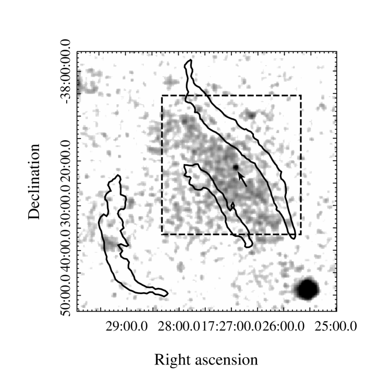
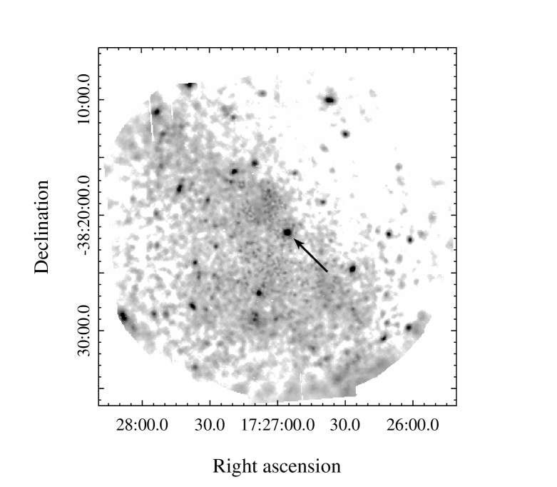
Figure 1: ROSAT 58 arcmin$\times$58 arcmin G350.0$-$2.0 field in 0.1–2.4 keV band (left panel) together with the VLA 1.4 GHz radio contours (Gaensler, 1998). 31 arcmin$\times$31 arcmin exposure and vignetting corrected QPB-subtracted XMM-Newton image in 0.4–7.2 keV band is shown in the right panel (the data of MOS and pn detectors are combined). The respective region is shown in the left panel with the dashed square. Square root brightness scale is used for both images. The X-ray source J1726 is marked by the arrows.

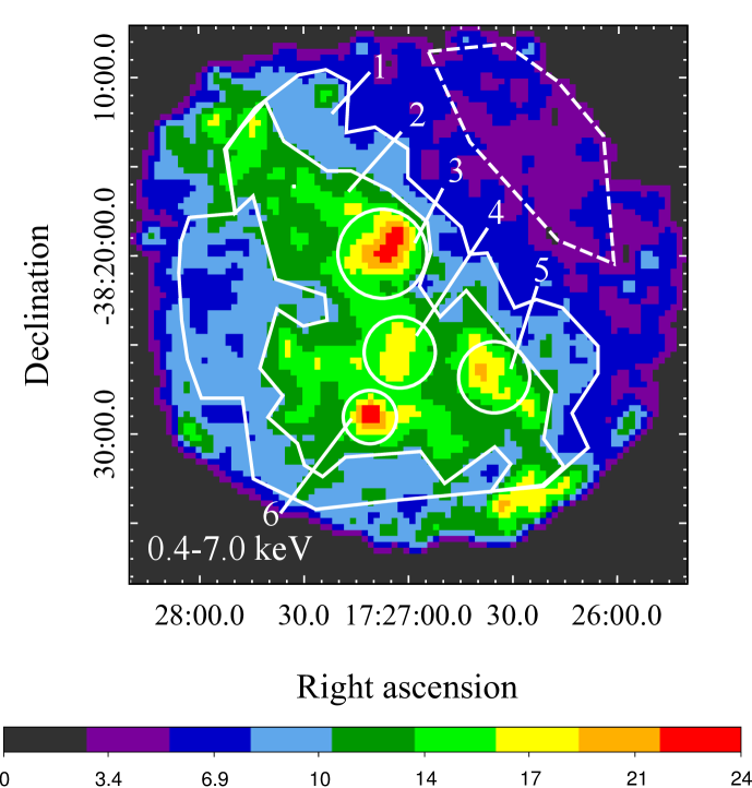
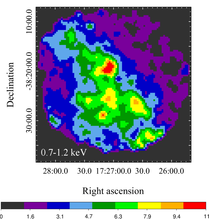
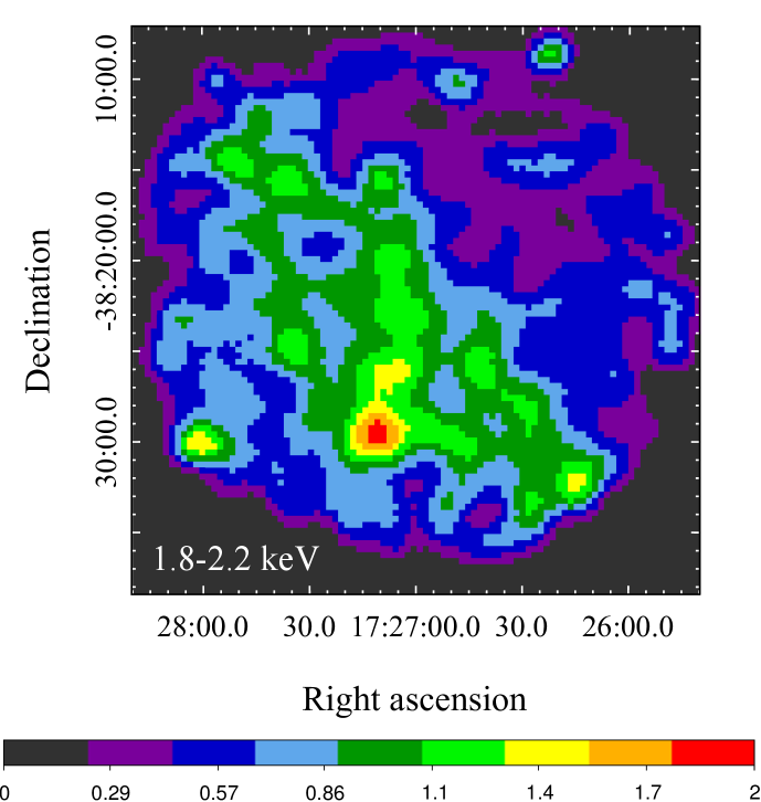
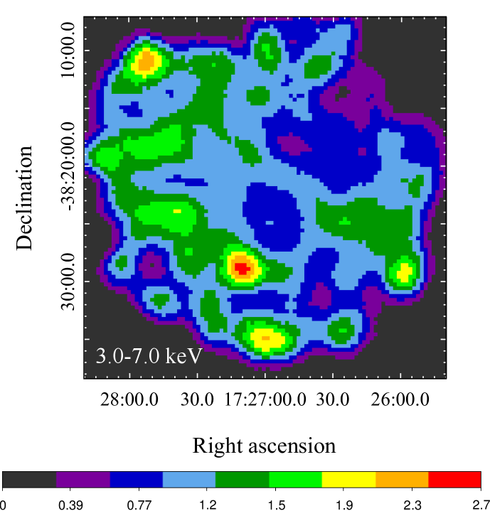
Figure 2: G350.0$-$2.0 images in 0.4–7 keV (top left), 0.7–1.2 keV (top right), 1.8–2.2 keV (bottom left) and 3–7 keV (bottom right) energy bands. The data of MOS and pn detectors are combined. The images are exposure and vignetting corrected and QPB-subtracted. Point sources are removed. The pixel size is 20 arcsec. The intensity is given in counts s^-1 deg^-2. In the top left panel, regions used for spectral analysis are shown (see text for details).

SNR G350.0$-$2.0 was discovered in the radio with Molonglo and Parkes telescopes at 408 MHz and 5 GHz, respectively (Caswell et al., 1975). Very Large Array (VLA) observations (Gaensler, 1998) showed complicated morphology of G350.0$-$2.0 that consists of three spatially distinct emission regions: the bright north-western and fainter inner and south-eastern arcs (Fig. 1, left panel). The whole extent of G350.0$-$2.0 in the radio is $\sim 40$ arcmin. In the optical, Stupar & Parker (2011) found some H$\alpha$ filaments and clumps spatially coinciding with the radio structures. G350.0$-$2.0 was observed in X-rays with ROSAT and ASCA. The multiwavelength data show that the SNR belongs to the MM SNR type (see Fig. 1, left panel). The age of the SNR was estimated as $\sim 10^{4}$ yr assuming the Sedov expansion phase (Helfand, Chanan & Novick, 1980; Clark & Stephenson, 1975). Basing on the radio surface brightness-to-diameter relationship, Case & Bhattacharya (1998) estimated the distance $D$ to G350.0$-$2.0 to be about 3.7 kpc.

A bright X-ray point-like source, 1RXS J172653.4$-$382157 (hereafter J1726), was detected in the SNR field with ROSAT (see Fig. 1, left panel) and ASCA. It may be an associated neutron star (NS) although no radio pulsar was detected within the SNR (Kaspi et al., 1996). On the other hand, it may be an unrelated object. To study the SNR and J1726 properties, we performed XMM-Newton observations. Here we present results of the analysis of the G350.0$-$2.0 and J1726 X-ray emission. The details of observations and imaging are described in Section 2. The analysis of the X-ray SNR spectra is presented in Section 3. J1726 is analysed in Section 4. We discuss results in Section 5 and summarise them in Section 6.

2 X-ray data and imaging

The XMM-Newton observations of G350.0$-$2.0 were carried out on 2013 September 21 with total exposure of about 38 ks. The telescope was pointed to the J1726 position. The EPIC field of view covers almost whole diffuse emission seen with ROSAT in the north-western part of the SNR (Fig. 1, left panel). All EPIC cameras were operated in the Full Frame Mode with the medium filter setting. The xmm-sas v.13.5.0 software was used to analyse the data. Data were reprocessed using the SAS tasks emchain and epchain.

We used the XMM-Newton Extended Source Analysis Software(esas; Snowden & Kuntz, 2014) to analyse the SNR emission. Utilizing mos-filter and pn-filter tools, we filtered out bad time intervals caused by soft proton flares. The resulting exposures are 19.5, 21.3 and 15.8 ks for EPIC-MOS1, MOS2 and pn, respectively. To identify whether any MOS CCD was in an anomalous state, we ran emtaglenoise task. MOS2 CCD #5 showed enhanced background below 1 keV and was excluded from further analysis. MOS1 CCDs #3 and #6 were damaged by micrometeorite strikes and are no longer functional (Snowden & Kuntz, 2014). Therefore, MOS1 does not cover the entire SNR region and was not used for the spectral analysis of G350.0$-$2.0 emission. We selected single and double pixel events (PATTERN $\leq$ 4) for the EPIC-pn and single to quadruple-pixel events (PATTERN $\leq$ 12) for the EPIC-MOS data. Images were created by mos-spectra and pn-spectra tasks. mos_back and pn_back routines were run to create the quiescent particle background (QPB) images. Then MOS and pn QPB-subtracted images were combined and adaptively smoothed. The resulting image in 0.4–7.2 keV energy range is shown in the right panel of Fig. 1. The shape of diffuse emission is generally consistent with that seen in the ROSAT image presented in the left panel. However, deeper XMM-Newton observation revealed many point-like sources in the SNR field. We also constructed images for 0.4–7, 0.7–1.2, 1.8–2.2 and 3–7 keV bands to investigate spectral variations of the SNR morphology. In these images, point-like sources were removed using cheese tool and MOS and pn images were combined and binned using bin_image task. The resulting images are shown in Fig. 2. We did not find any evidence of the X-ray counterparts of the radio shells. The most prominent structures are blobs 3–6 found in the inner part of the diffuse emission; they are marked in the top left panel of Fig. 2. Blobs 3–5 reveal themselves brighter in the 0.7–1.2 keV band where the Fe-L emission dominates in the SNR spectrum. Blob 6 seems to have the spectrum different from the rest of the SNR since its emission is harder.

3 Spectral analysis of G350.0$-$2.0

Table 1: Best-fit parameters for the absorbed vapec model for the SNR emission from different regions. Parameters for additional Gaussian component for regions 1–5 and for power law emission for the region 6 are also given (see text for details). Errors are at 90% confidence.

Region	1	2	3	4+5	6
Column density $N_{\rm H}$, $10^{21}$ cm-2	$7.1^{+0.5}_{-0.6}$	$6.2^{+0.3}_{-0.3}$	$7.2^{+2.0}_{-1.5}$	$6.6^{+1.4}_{-1.4}$	$5.3^{+1.6}_{-1.2}$
Temperature $T$, keV	$0.85^{+0.05}_{-0.04}$	$0.82^{+0.02}_{-0.02}$	$0.85^{+0.04}_{-0.05}$	$0.84^{+0.03}_{-0.05}$	$0.85^{+0.05}_{-0.08}$
VEM, $10^{56}D^{2}_{\rm 3.7kpc}$ cm-3 a	$3.1^{+0.4}_{-0.3}$	$4.1^{+0.4}_{-0.4}$	$0.5^{+0.1}_{-0.1}$	$0.7^{+0.1}_{-0.1}$	$0.2^{+0.1}_{-0.1}$
Fe/Fe⊙	1.0 (fixed)	1.0 (fixed)	$2.3^{+2.3}_{-1.0}$	$1.8^{+1.0}_{-0.7}$	1.0 (fixed)
Gaussian energy $E$, keV	$1.26^{+0.02}_{-0.02}$	$1.26^{+0.01}_{-0.01}$	$1.23^{+0.04}_{-0.04}$	$1.24^{+0.04}_{-0.03}$
Gaussian width $\sigma$, keV	$0.05^{+0.02}_{-0.03}$	$0.07^{+0.01}_{-0.01}$	$0.08^{+0.05}_{-0.07}$	$0.08^{+0.04}_{-0.05}$
Gaussian normalization $K$, $10^{-4}$ ph cm-2 s-1	$0.9^{+0.4}_{-0.3}$	$1.8^{+0.3}_{-0.3}$	$0.6^{+0.3}_{-0.3}$	$0.5^{+0.2}_{-0.2}$
Photon index $\Gamma$					$1.8^{+0.7}_{-1.2}$
PL normalization $N_{\rm PL}$, $10^{-5}$ ph cm-2 s-1 keV-1					$2.2^{+2.9}_{-1.8}$
$\chi^{2}$/d.o.f.b	1063/1001		265/261	338/320	74/67

• ^a VEM is the volume emission measure defined in equation (1) and $D_{\rm 3.7kpc}$ is the distance in units of 3.7 kpc.

• ^b d.o.f. = degrees of freedom.

We extracted the SNR spectra from MOS2 and pn data and created redistribution matrix and ancillary response files using mos-spectra and pn-spectra tools. The extraction regions are shown in the top left panel of Fig. 2. The outer region 1 was chosen on the overlapping part of MOS2 and pn fields of view between contour levels of 7.5 and 11 cnt s^-1 deg^-2. The region 2 corresponds to the central part of the remnant with brightness $>$11 cnt s^-1 deg^-2. Bright regions 3–6 were excluded from the region 2 and analysed separately. MOS2 and pn spectra were grouped to ensure $>50$ and $>20$ counts per energy bin for regions 1–2 and 3–6, respectively. Unfortunately, we could not obtain the astrophysical background spectrum for MOS2 data since the only appropriate region was exposed on CCD #5 which was in anomalous mode. Thus, it was extracted only from the pn data (from the dashed polygon region depicted in Fig. 2, top left panel). The background spectrum was binned with a minimum of 50 counts per bin.

The spectra were fitted in the 0.4–7 keV range to exclude strong pn instrumental Ni-K$\alpha$, Cu-K$\alpha$ and Zn-K$\alpha$ lines which contaminate harder part of the spectra. Two Gaussians (model gauss in xspec) with energies of $\sim 1.5$ and $\sim 1.75$ keV were used to describe Al-K$\alpha$ and Si-K$\alpha$ instrumental lines. For the astrophysical background, we used the model consisting of a cool unabsorbed thermal component with temperature of 0.1 keV for the emission from the Local Bubble, two absorbed thermal components for the emission from the cooler and hotter Galactic halo, and an absorbed power law with $\Gamma=1.46$ describing the unresolved background of cosmological sources (see Snowden & Kuntz, 2014). Additional power law components not convolved with the instrumental response were utilized to account for the residual soft proton (SP) contamination. We set limits on the photon indices of these components at 0.1 and 1.4 following the esas Cookbook (Snowden & Kuntz, 2014). For the interstellar absorption, we used the xspec photoelectric absorption phabs model with solar abundances of Anders & Grevesse (1989).

For the SNR emission, we used the collisionally-ionized equilibrium plasma model vapec. Spectra of regions 1, 2 and astrophysical background were fitted simultaneously. The excess in residuals was seen near the energy of 1.25 keV which we could not remove varying abundances so we added a Gaussian component to the vapec model. The best-fit parameters are presented in Table 1 and the best-fit model is shown in Fig. 3. Parameters of astrophysical background obtained from this fit were then used for fitting spectra of regions 3–6.

For the bright regions 3–5, the vapec model with solar abundances does not fit the spectra well. The best fits (see Table 1) indicate an overabundance of iron. As for the regions 1–2, the additional Gaussian component is needed to remove the excess in residuals at 1.25 keV. Notice, that the regions 4 and 5 were fitted simultaneously.

The single vapec model did not provide a satisfactory fit for the emission from region 6 ($\chi^{2}$/d.o.f. = 88/69). The addition of a power law (PL) component improved the fit (see Table 1). The addition of Gaussian component at 1.25 keV is not needed to describe the spectra possibly due to a low count number.

The physical nature of the additional Gaussian component at 1.25 keV is not clear. The central energy formally corresponds to Mg XI K-lines, but variation of the Mg abundance did not remove the excess in residuals. Alternatively, it can be interpreted as emission of Fe-L lines originating from energy levels with high principal quantum numbers (e.g. Brickhouse et al., 2000; Yamaguchi et al., 2011). This is supported by a positive correlation between line equivalent width $\propto K/$VEM, where $K$ is the Gaussian normalization and VEM is the volume emission measure (see Table 1), and the abundance of Fe found in different regions, see Table 1. While sufficient number of transitions is included in the current release of the atomdb (v.3.0.3) used for the vapec model, it is possible that the description of the Fe-L complex is still incomplete.

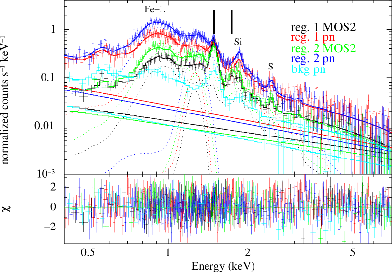
Figure 3: Top: XMM-Newton EPIC spectra of G350.0$-$2.0 emission from regions 1–2 and the background region. Lines represent the best-fit model, assuming vapec+gauss components for the SNR emission (see text for details). Solid inclined lines represent the SP contamination, dotted lines – vapec and gauss components. Different instruments/regions are shown by different colors as indicated in the top right corner. The instrumental lines positions are shown by thick bars. Emission features of Fe-L, Si and S are indicated. Bottom: fit residuals.

4 Analysis of J1726

4.1 Timing

For the timing analysis of J1726, we used EPIC-pn data with the time resolution of 73.4 ms. We extracted events from the 30 arcsec radius aperture in 0.3–10 keV range and corrected them to the solar system barycentre using barycen tool and J1726 coordinates obtained with edetect_chain task (RA = $261\hbox{$.\!\!^{\circ}$}7334$, Dec = $-38\hbox{$.\!\!^{\circ}$}3595$). $Z^{2}_{n}$ test (Buccheri et al., 1983) was used to search for pulsations with periods in the 0.15–4000 s range. The number of harmonics $n$ was varied from 1 to 5. No pulsations were found. An upper limit for the pulsed fraction (PF) of 27% (at the 99% confidence level) was estimated following Brazier (1994) and adopting $n=1$.

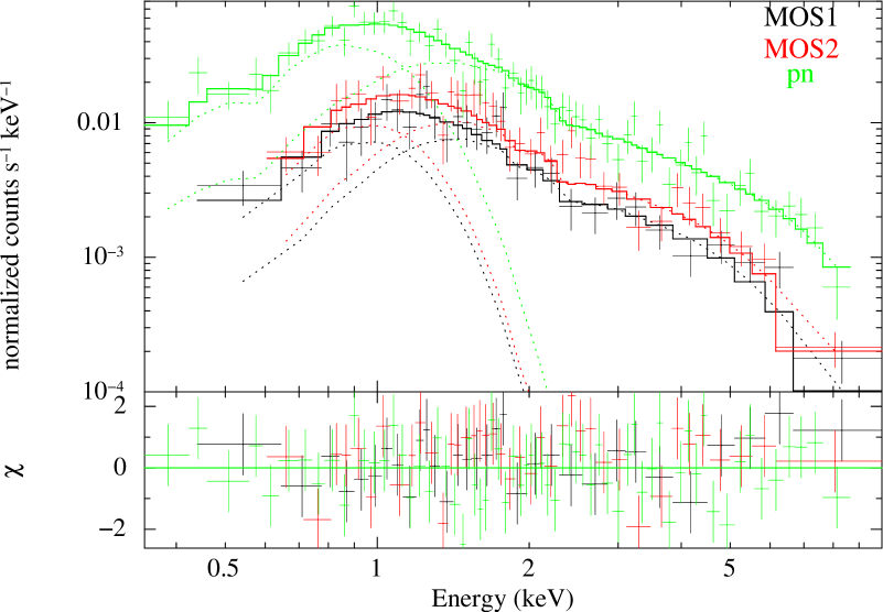
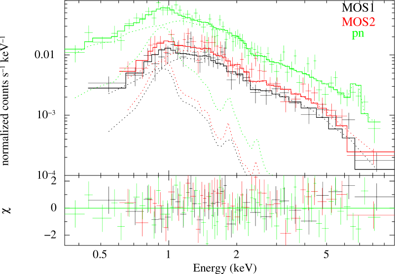
Figure 4: XMM-Newton EPIC spectra of the J1726 best-fitted with PL+BB (top) and 2-T mekal (bottom) models and fit residuals. Different instruments are shown by different colors as indicated in the top right corners. Dotted lines represent model components.

4.2 X-ray spectra

We extracted the J1726 spectra from MOS1, MOS2 and pn data from the 30 arcsec radius aperture using evselect tool. The 45–75 arcsec annulus region around J1726 was chosen for the background extraction. The resulting number of source counts was 410(MOS1)+625(MOS2)+1340(pn). sas tasks rmfgen and arfgen were utilized to generate the redistribution matrix and ancillary response files. Spectra were grouped to ensure $>15$ counts per energy bin and then fitted simultaneously in the 0.3–10 keV range.

Assuming the NS origin of J1726, we applied the absorbed power law (PL), power law plus blackbody (PL+BB) and power law plus the magnetized hydrogen atmosphere (PL+NSA; Pavlov et al., 1995) models. The PL component describes the magnetospheric emission while BB or NSA refer to the thermal emission from the NS surface. We also tried the absorbed two-temperature optically thin thermal plasma (mekal) model (Mewe, Gronenschild & van den Oord, 1985) which is usually used to describe spectra of cataclysmic variables (CVs) (see, e.g., Baskill et al., 2005; Reis et al., 2013). The cooler component describes the emission from the unshocked accretion flow and white dwarf photosphere while the hotter one describes the shocked flow emission. The results are presented in Table 2. According to $\chi^{2}$ values, all models describe the data well.

The F-test was applied to investigate whether the thermal component is required to describe the soft part of the spectra if J1726 is a NS. It gave a probability of chance improvement of $\approx 10^{-6}$, showing that the thermal component is needed. The fits for the PL+BB and 2-T mekal models are shown in Fig. 4. The derived photon index $\Gamma$ and the BB temperature are typical for pulsar emission. For the distance of 3.7 kpc, the emitting area radius is consistent within uncertainties with a canonical NS radius of about 15 km. At the same time, the hydrogen atmosphere model NSA with NS mass $M_{\rm NS}=1.4M_{\odot}$ and radius $R_{\rm NS}=13$ km can equally well describe the thermal component.

For the 2-T mekal model, the obtained temperatures of 0.8 and 8.6 keV are typical for CVs (see e.g. Heinke et al., 2005). The single temperature mekal model was rejected by the worse fit ($\chi^{2}$/d.o.f.=157/135).

Table 2: J1726 best-fit spectral parameters for different models. All errors correspond to 90% confidence intervals. Unabsorbed fluxes $f_{\rm X}$ refer to the 0.3–10 keV energy range. For the PL+NSA model, the magnetic field $B=10^{12}$ G, the NS mass $M_{\rm NS}=1.4M_{\odot}$, the NS radius $R_{\rm NS}=13$ km, the distance to the object $D$ was fixed at 3.7 kpc and the temperature is given as seen by a distant observer. $N_{\rm PL}$ is the PL normalization component.

Parameters/	$N_{\rm H}$,	$\Gamma$	$N_{\rm PL}$,	$T$,	$R$,	$T_{1}$,	$T_{2}$,	$f_{\rm X}$,	$\chi^{2}$/d.o.f.
Model	1021 cm-2		10-5 ph keV-1 cm-2 s-1	eV	km	keV	keV	10-13 erg s-1 cm-2
PL	$2.4^{+0.4}_{-0.3}$	$1.81^{+0.12}_{-0.11}$	$7.8^{+1.0}_{-0.9}$					5.0	146/135
PL+BB	$5.1^{+2.0}_{-1.7}$	$1.71^{+0.20}_{-0.20}$	$7.3^{+2.3}_{-1.8}$	$138^{+42}_{-25}$	$5^{+10}_{-3}$ $D_{\rm 3.7kpc}$			10.2	119/133
PL+NSA	$4.3^{+0.4}_{-0.4}$	$1.60^{+0.14}_{-0.14}$	$6.1^{+1.1}_{-1.0}$	$73^{+3}_{-3}$	13 (fixed)			8.3	122/134
2-T mekal	$2.0^{+0.4}_{-0.3}$					$0.8^{+0.3}_{-0.1}$	$8.6^{+4.1}_{-2.1}$	4.6	126/133

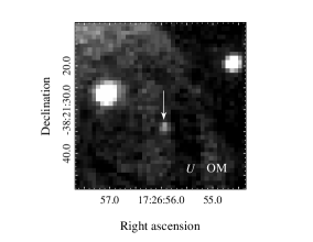
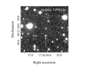
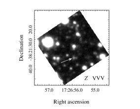
Figure 5: 0.65 arcmin$\times$0.65 arcmin optical/infrared images of the J1726 field. Filters and surveys are indicated in the images. The J1726 possible counterpart is marked by an arrow in each image.

4.3 UV and optical data

A faint optical source was detected at the J1726 position with the XMM-Newton Optical/UV Monitor (OM) (see Fig. 5, left panel) in the $U$ filter ($\lambda_{\rm eff}=344$ nm). It can be the J1726 counterpart. Using the omdetect task, we obtained the background-subtracted count rate of 0.15 cts s^-1 that corresponds to the instrumental magnitude $U=20.35\pm 0.19$ ($U_{AB}\approx 21.28\pm 0.19$). We note that this value should be considered with caution since the source was on top of a prominent arc of straylight artefact seen as diffuse emission in Fig. 5 that prevents to measure its count rate accurately (XMM-Newton support team, private communication). The J1726 field was also observed in $V$, $UVM2$ and $UVW1$ filters but the source was not detected in these bands.

At the same time, the source was found in archival images obtained in the VISTA Variables in the Via Lactea Survey (VVV; PI Dante Minniti; Minniti et al., 2010) and the VST Photometric H$\alpha$ Survey of the Southern Galactic Plane and Bulge (VPHAS+; PI Janet Drew; Drew et al., 2014). In these surveys, the source is catalogued as VPHASDR2 J172655.9$-$382134.4 and VVV J172655.88$-$382134.20. Examples of VPHAS+ H$\alpha$ and VVV $Z$ images are shown in the middle and right panels of Fig. 5, respectively. The source coordinates obtained in different surveys are fully consistent with the X-ray position of J1726 obtained with the nominal XMM-Newton pointing accuracy of 2 arcsec (90% confidence).

Visual magnitudes and observed fluxes measured in different bands are presented in Table 3. $Z$, $Y$, $J$, $H$ and $K_{s}$ magnitudes were obtained from VVV catalogue for 1 arcsec aperture. Since the field is very crowded in the infrared band (see Fig. 5, right panel), we checked the VVV catalogue values using iraf. The derived values were in agreement with the catalogue ones within uncertainties. Nevertheless, the source emission is contaminated by nearby stars and flux values may be overestimated. VPHAS+ catalogue provides $u$, $g$, $r$, H$\alpha$ and $i$ magnitudes obtained using point spread function (PSF) fitting and aperture photometry. Both methods give consistent results. The former values are presented in Table 3. The source of interest was observed at two epochs. At MJD 56566, observations were performed in $u$, $g$ and $r$ filters and at MJD 56149 – in $r$, H$\alpha$ and $i$ filters. In addition, two scans, primary and duplicate, are provided for each epoch. As noted in the catalogue description, the primary detection is the one for which the magnitude could be measured successfully in the largest number of filters.

5 Discussion

5.1 The remnant

The spectra of the most part of the SNR can be fitted with vapec+gauss model except for the region 6 where the additional PL component is required. As can be seen from Table. 1, temperatures and absorption column densities obtained for different parts of the SNR are consistent with each other within uncertainties. Plasma in regions 1–2 has solar abundances suggesting that the emission comes from the shocked interstellar medium that is typical for MM SNRs (Rho & Petre, 1998). However, the analysis of bright regions 3–5 revealed the overabundance of Fe in these regions which may indicate the presence of ejecta material. Alternatively, the metal enrichment can be provided by the dust destruction (see e.g. Shelton et al., 2004).

The measured $N_{\rm H}$ value (Table 1) allows to independently estimate the distance to the remnant. The empirical $N_{\rm H}$–$A_{V}$ relation (Güver & Özel, 2009) results in the optical extinction $A_{V}\approx 3$ assuming $N_{\rm H}=6.5\times 10^{21}$ cm^-2. Using $A_{V}$–distance fit from Drimmel, Cabrera-Lavers & López-Corredoira (2003), we got $D\approx 3$ kpc that is compatible with $D=3.7$ kpc obtained by Case & Bhattacharya (1998) from the radio surface brightness. For the distance of 3.7 kpc, the SNR radius is about 20 pc.

The gas number density can be calculated from the vapec model normalization given as

$$N=\frac{10^{-14}}{4\pi D^{2}_{\rm cm}}\int n_{e}n_{\rm H}dV\equiv\frac{10^{-14}}{4\pi D^{2}_{\rm cm}}\times{\rm VEM},$$ (1)

where $n_{e}$ and $n_{\rm H}$ are the electron and hydrogen number densities, respectively, $D_{\rm cm}$ is the distance in centimetres and VEM is the volume emission measure. For solar abundances, $n_{e}=1.2n_{\rm H}$ assuming almost complete ionization. The volume of the particular X-ray emitting region was estimated as $V=7.3\times 10^{56}SL_{20}D_{\rm 3.7kpc}^{2}$ cm³, where $S$ is the area of this region in arcmin² and $L_{20}$ is its extension along the line of sight in the units of 20 pc. Then

$$n_{\rm H}=13.6N^{1/2}(SL_{20})^{-1/2}.$$ (2)

The resulting $n_{\rm H}$ values are presented in Table 4 together with the masses of the emitting gas $M_{g}$ calculated assuming mean atomic weight for solar abundances $\mu=0.604$. The number density distribution seems to be rather uniform though it depends on the volume estimation. The total gas mass is about 15$M_{\odot}$ if we assume identical extensions of 20 pc for all regions.

Table 3: Visual magnitudes, observed and dereddened fluxes of the J1726 possible optical counterpart obtained from different surveys. Dereddening was done with the interstellar absorption $A_{V}$ = 0.9 assuming 2-T mekal X-ray spectral model (see text for details).

Filter	$\lambda_{\rm eff}$, $\mu$m	MJD	Magnitude	Flux, $\mu$Jy	Dereddened flux, $\mu$Jy
$U$(OM)	0.344	56556.83866	$20.35\pm 0.19$	$11\pm 2$	$41.7\pm 7.6$
$u$	0.361	56566.01030a	$19.81\pm 0.07$	$17.8\pm 1.2$	$65.8\pm 4.4$
		56566.01254b	$19.74\pm 0.07$	$19.0\pm 1.2$	$70.3\pm 4.4$
$g$	0.468	56566.02029a	$21.04\pm 0.05$	$15.7\pm 0.7$	$42.1\pm 1.9$
		56566.02224b	$21.17\pm 0.05$	$13.8\pm 0.7$	$37.0\pm 1.9$
$r$	0.624	56566.02705a	$20.33\pm 0.06$	$23.7\pm 1.3$	$48.6\pm 2.7$
		56566.02785b	$20.51\pm 0.08$	$20.0\pm 1.5$	$41.0\pm 3.1$
		56149.08459a	$20.58\pm 0.06$	$18.8\pm 1.0$	$38.6\pm 2.1$
		56149.08535b	$20.66\pm 0.06$	$17.5\pm 1.0$	$35.9\pm 2.1$
H$\alpha$	0.659	56149.07406a	$19.13\pm 0.04$	$55.4\pm 2.1$	$108.5\pm 4.3$
$i$	0.760	56149.09070a	$20.02\pm 0.06$	$25.4\pm 1.4$	$43.6\pm 2.4$
		56149.09146b	$19.76\pm 0.07$	$32.1\pm 2.0$	$55.2\pm 3.4$
$Z$	0.878	55725.26322	$18.97\pm 0.09$	$58.2^{+5.2}_{-4.8}$	$87.6^{+7.9}_{-7.3}$
$Y$	1.021	55725.25799	$19.05\pm 0.13$	$50.3^{+6.5}_{-5.8}$	$78.3^{+9.0}_{-8.0}$
$J$	1.254	55309.36337	$18.55\pm 0.13$	$58.9^{+7.7}_{-6.8}$	$74.3^{+9.8}_{-8.6}$
$H$	1.646	55309.35370	$17.87\pm 0.17$	$73.1^{+12.5}_{-10.7}$	$84.9^{+14.5}_{-12.4}$
$K_{s}$	2.149	55309.35857	$17.51\pm 0.20$	$66.9^{+13.3}_{-11.1}$	$73.8^{+14.7}_{-12.2}$

• ^a Primary observation.

• ^b Duplicate observation.

Table 4: The hydrogen number densities $n_{\rm H}$ and masses of the emitting gas $M_{g}$ for the different SNR regions.

Region	$n_{\rm H}$,	$M_{g}$,
	10${}^{-2}L_{20}^{-1/2}$ cm-3	$L_{20}^{1/2}D_{\rm 3.7kpc}^{2}M_{\odot}$
1	$4.7^{+0.4}_{-0.3}$	$6.2^{+0.5}_{-0.4}$
2	$5.9^{+0.3}_{-0.3}$	$6.5^{+0.3}_{-0.3}$
3	$5.4^{+0.7}_{-0.5}$	$0.9^{+0.1}_{-0.1}$
4+5	$5.4^{+0.6}_{-0.5}$	$1.1^{+0.1}_{-0.1}$
6	$5.4^{+1.8}_{-1.2}$	$0.3^{+0.1}_{-0.1}$

G350.0$-$2.0 has a complicated non-spherically symmetric morphology which is similar to that of the SNR G166.0+4.3 (see e.g. Bocchino et al., 2009). Both SNRs show three radio emitting arcs while the X-ray emission fills the part of the volume enclosed within two arcs. The G166.0+4.3 radio morphology was explained Pineault et al. (1987) as follows. The supernova explodes in a moderately dense medium and then the SN shock passes through a low-density cavity (hot tunnel). Gaensler (1998) suggested the similar model for G350.0$-$2.0. The inner arc is then formed at the boundary of the cavity. This implies that the observed X-ray emission fills the low-density region, in qualitative accordance with the $n_{\rm H}$ values in Table 4.

The spatially-resolved spectral analysis showed the uniform temperature distribution over the remnant. This is consistent with the predictions of the thermal conduction model (e.g. Cox et al., 1999). The conduction timescale can be estimated as

$$t_{\rm cond}\sim 27\frac{n_{e}}{1\ {\rm cm}^{-3}}\left(\frac{l_{T}}{10\ {\rm pc}}\right)^{2}\left(\frac{T}{0.8\ {\rm keV}}\right)^{-2.5}\frac{{\rm ln}\Lambda}{33}\ {\rm kyr},$$ (3)

where $l_{T}=T/\nabla{T}$ is the scale length of the temperature gradient and ln$\Lambda=29.7+{\rm ln}n_{e}^{-0.5}(T/0.086\ {\rm keV})$ is the Coulomb logarithm. For $l_{T}\approx 20$ pc, $t_{\rm cond}\sim 7$ kyr is less than the estimated Sedov age of G350.0$-$2.0 (Helfand et al., 1980; Clark & Stephenson, 1975). Therefore thermal conduction may play a role in smoothing the temperature distribution. Direct comparison with results obtained by Cox et al. (1999) is difficult since their solutions are constructed assuming spherical symmetry which is not the case of G350.0$-$2.0.

There exist simulations of the X-ray emission for MM SNRs evolving in the non-uniform density medium. For example, Schneiter et al. (2006) presented simulations for the SNR 3C 400.2 assuming the SNR evolution in the medium with a jump in the density and taking into account the effects of thermal conduction and interstellar absorption. Their results for the SNR explosion at the denser side or at the density interface show the X-ray emission pattern remarkably similar to that observed in G350.0$-$2.0 (see their Fig. 4). Thus, the G350.0$-$2.0 morphology may be qualitatively explained assuming its evolution in a multi-component interstellar medium. However, detailed numerical simulations are required.

The cloudlet evaporation model of White & Long (1991) is also frequently used to explain MM SNR properties. This model predicts the radial density gradient which is not observed for G350.0$-$2.0 (Table 4). However, this cannot be considered as a solid argument since the model predictions for the non-spherically symmetric case can be different.

5.2 The region 6

The emission from the region 6 is harder than that from the rest of the SNR and the additional power law component is needed to describe its spectrum. Two weak point sources are presented inside the region 6. The first one (RA = $261\hbox{$.\!\!^{\circ}$}790$, Dec = $-38\hbox{$.\!\!^{\circ}$}478$) shows a softer emission (it is not seen in 3–7 keV image). A possible optical counterpart was found for this source in the USNO-B1.0 catalogue (ID 0515$-$0517969), OM, VPHAS+ and VVV images. The second source (RA = $261\hbox{$.\!\!^{\circ}$}794$, Dec = $-38\hbox{$.\!\!^{\circ}$}485$) has hard emission and does not have an optical counterpart. It is possible that the PL emission results from the incomplete subtraction of this source by cheese task. We tried to use larger aperture of 30 arcsec to mask the source but this did not remove the PL component. On the other hand, extracting spectra of the region 6 including point sources and fitting them with vapec+PL model resulted in a similar $\Gamma=1.9\pm 0.5$ and a larger PL normalization $N_{\rm PL}=(4.3\pm 2.5)\times 10^{-5}$ ph cm^-2 s^-1 keV^-1 than in previous case (Table 1). The unabsorbed 0.3–10 keV flux in the PL component changed from 1.4$\times$10^-13 to 2.6$\times$10^-13 erg cm^-2 s^-1. For $D=3.7$ kpc, these numbers correspond to the X-ray luminosity in the range of $(2-5)\times 10^{32}$ erg s^-1. The obtained PL parameters are typical for pulsar+pulsar wind nebula (PWN) systems with ages $\gtrsim 10$ kyr (Kargaltsev & Pavlov, 2008). This together with the spatial extent of the region 6 of $1-2$ arcmin allows us to suggest it as a PWN candidate. However, we do not see any diffuse emission that resembles a PWN in the VLA 1.4 GHz image though it may be blended with the emission of the inner arc.

As an alternative, to check if the hard emitting component in the region 6 may have a thermal origin, we fitted its spectrum with a vapec$+$vapec model. The fit is acceptable with $\chi^{2}$/d.o.f. = 75/67 and suggests the presence of warm and hot plasma components. Within uncertainties, the warm vapec component has the same parameters as in the vapec$+$PL case, while the best fit temperature for the hot component is about 12 keV with a 90% lower limit of 3.6 keV. This is atypical for SNRs where the second hot thermal component, if observed, has a temperature of $\la$ 3 keV (e.g. Kawasaki et al., 2005) and makes the thermal interpretation of the hard component less plausible especially for an evolved SNR such as G350.0$-$2.0.

5.3 J1726

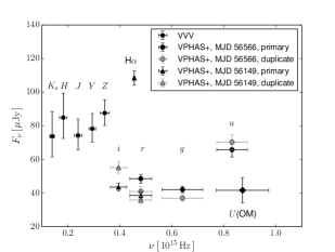
Figure 6: Dereddened flux density vs. frequency for the J1726 possible counterpart taken from Table 3. Data points for different observations are shown by different symbols as indicated in the inset.

The J1726 X-ray spectrum is well described by PL+BB(NSA) model with parameters typical for rotation powered pulsars. The corresponding column density is consistent within uncertainties with that of the SNR supporting the NS origin of the source. The detection of pulsations could confirm this, but pulsations were not found (Section 4). The derived upper limit for PF of 27% is non-informative since PFs of many NSs are lower than this value. Moreover, the actual period for the putative NS can be smaller than the Nyquist limit for our observations of $\approx 150$ ms. Higher time resolution observations are required to solve this problem.

An optical source with a non-stellar spectral energy distribution was found at the X-ray position of J1726. Assuming that the optical source is the J1726 counterpart, we calculated the X-ray to optical flux ratio $f_{\rm X}/f_{g}$. The magnitude $g$ was corrected for interstellar extinction adopting the extinction law of Cardelli, Clayton & Mathis (1989) and $A_{V}=3$ (see Subsection 5.1). The unabsorbed X-ray flux was obtained in the 0.3–10 keV energy band (Table 2). We got $f_{X}/f_{g}\approx 1.5$. This is less than the values obtained for low-mass X-ray binaries ($\sim 10^{2}-10^{3}$) or isolated NSs ($\gtrsim 10^{3}$; Trümper & Hasinger, 2008). While a chance spatial coincidence of a NS and an unrelated optical source can not be ruled out, the NS interpretation seems to be unlikely.

On the other hand, the spectral energy distribution of the putative optical counterpart points to the CV interpretation. This is also supported by J1726 X-ray spectrum, which is well described by the two-temperature optically thin plasma model typical for CVs (Baskill et al., 2005; Reis et al., 2013). The dereddened optical fluxes obtained in different bands are presented in the last column of Table 3 and shown in Fig. 6. The dereddening was performed using $A_{V}=0.9$ which corresponds to $N_{\rm H}$=2$\times$10²¹ cm^-2 obtained from the 2-T mekal fit. The optical source shows a flux excess in a narrow-band H$\alpha$ filter (Table 3) that is a common feature for CVs (see, e.g., Witham et al., 2006). The X-ray to optical flux ratio $f_{X}/f_{g}\approx 7$ is also usual for CVs (La Palombara et al., 2006).

Other interpretations of the J1726 nature are less plausible. For instance, J1726 cannot be an AGN since $N_{\rm H}$ obtained for the single PL fit, typical for AGNi, is much smaller than the total Galactic $N_{\rm H}$ in this direction of $9.5\times 10^{21}$ cm^-2 derived from the H i map by Dickey & Lockman (1990).

6 Summary

We analysed the XMM-Newton observations of the Galactic MM SNR G350.0$-$2.0. We showed that the spectrum of the most part of the SNR is well described by the vapec model with solar abundances suggesting that the X-ray emission originates from the shocked interstellar material. However, the analysis of some bright regions revealed an overabundance of Fe possibly indicating the presence of ejecta. No temperature variations over the observed part of the remnant were found indicating that thermal conduction effects may be important. The complicated multiwavelength morphology of G350.0$-$2.0 can be explained assuming its evolution in the medium with jumps in the density. Deeper X-ray observations are required to investigate the properties of the entire SNR. The X-ray spectra of the brightest source J1726 in the SNR field can be fitted either by PL+BB(NSA) or 2-T mekal models. In the former case, the best-fit parameters are typical for a rotation powered pulsar and the absorption column density is in agreement with the SNR one although no pulsed emission was detected with PF upper limit of 27%. Alternatively, J1726 is a foreground source, likely a CV. The latter possibility is supported by a faint optical source with a non-stellar spectrum found at the J1726 X-ray position. It is possible that one of other point sources detected in the SNR field can be an associated compact object, however current X-ray data do not allow to reliably define their nature. For instance, the source with hard emission in region 6 is promising in this respect. Deeper X-ray observations with better spatial and timing resolution are needed to investigate it more accurately.

References

- Anders & Grevesse (1989) Anders E., Grevesse N., 1989, Geochimica Cosmochimica Acta, 53, 197
- Baskill et al. (2005) Baskill D. S., Wheatley P. J., Osborne J. P., 2005, MNRAS, 357, 626
- Bocchino et al. (2009) Bocchino F., Miceli M., Troja E., 2009, A&A, 498, 139
- Brazier (1994) Brazier K. T. S., 1994, MNRAS, 268, 709
- Brickhouse et al. (2000) Brickhouse N. S., Dupree A. K., Edgar R. J., Liedahl D. A., Drake S. A., White N. E., Singh K. P., 2000, ApJ, 530, 387
- Buccheri et al. (1983) Buccheri R., et al., 1983, A&A, 128, 245
- Cardelli et al. (1989) Cardelli J. A., Clayton G. C., Mathis J. S., 1989, ApJ, 345, 245
- Case & Bhattacharya (1998) Case G. L., Bhattacharya D., 1998, ApJ, 504, 761
- Caswell et al. (1975) Caswell J. L., Clark D. H., Crawford D. F., Green A. J., 1975, Australian Journal of Physics Astrophysical Supplement, 37, 1
- Clark & Stephenson (1975) Clark D. H., Stephenson F. R., 1975, The Observatory, 95, 190
- Cox et al. (1999) Cox D. P., Shelton R. L., Maciejewski W., Smith R. K., Plewa T., Pawl A., Różyczka M., 1999, ApJ, 524, 179
- Dickey & Lockman (1990) Dickey J. M., Lockman F. J., 1990, ARA&A, 28, 215
- Drew et al. (2014) Drew J. E., et al., 2014, MNRAS, 440, 2036
- Drimmel et al. (2003) Drimmel R., Cabrera-Lavers A., López-Corredoira M., 2003, A&A, 409, 205
- Gaensler (1998) Gaensler B. M., 1998, ApJ, 493, 781
- Güver & Özel (2009) Güver T., Özel F., 2009, MNRAS, 400, 2050
- Heinke et al. (2005) Heinke C. O., Grindlay J. E., Edmonds P. D., Cohn H. N., Lugger P. M., Camilo F., Bogdanov S., Freire P. C., 2005, ApJ, 625, 796
- Helfand et al. (1980) Helfand D. J., Chanan G. A., Novick R., 1980, Nat, 283, 337
- Kargaltsev & Pavlov (2008) Kargaltsev O., Pavlov G. G., 2008, in Bassa C., Wang Z., Cumming A., Kaspi V. M., eds, American Institute of Physics Conference Series Vol. 983, 40 Years of Pulsars: Millisecond Pulsars, Magnetars and More. pp 171–185 (arXiv:0801.2602), doi:10.1063/1.2900138
- Kaspi et al. (1996) Kaspi V. M., Manchester R. N., Johnston S., Lyne A. G., D’Amico N., 1996, AJ, 111, 2028
- Kawasaki et al. (2005) Kawasaki M., Ozaki M., Nagase F., Inoue H., Petre R., 2005, ApJ, 631, 935
- La Palombara et al. (2006) La Palombara N., Mignani R. P., Hatziminaoglou E., Schirmer M., Bignami G. F., Caraveo P., 2006, A&A, 458, 245
- Lazendic & Slane (2006) Lazendic J. S., Slane P. O., 2006, ApJ, 647, 350
- Mewe et al. (1985) Mewe R., Gronenschild E. H. B. M., van den Oord G. H. J., 1985, A&AS, 62, 197
- Minniti et al. (2010) Minniti D., et al., 2010, New Astronomy, 15, 433
- Pavlov et al. (1995) Pavlov G. G., Shibanov Y. A., Zavlin V. E., Meyer R. D., 1995, in Alpar M. A., Kiziloglu U., van Paradijs J., eds, The Lives of the Neutron Stars. Kluwer, Dordrecht, p. 71
- Pineault et al. (1987) Pineault S., Landecker T. L., Routledge D., 1987, ApJ, 315, 580
- Reis et al. (2013) Reis R. C., Wheatley P. J., Gänsicke B. T., Osborne J. P., 2013, MNRAS, 430, 1994
- Rho & Petre (1998) Rho J., Petre R., 1998, ApJ, 503, L167
- Schneiter et al. (2006) Schneiter E. M., de La Fuente E., Velázquez P. F., 2006, MNRAS, 371, 369
- Shelton et al. (2004) Shelton R. L., Kuntz K. D., Petre R., 2004, ApJ, 611, 906
- Snowden & Kuntz (2014) Snowden S. L., Kuntz K. D., 2014, Cookbook for analysis procedures for XMM-Newton EPIC observations of extendedobjects and the diffuse background
- Stupar & Parker (2011) Stupar M., Parker Q. A., 2011, MNRAS, 414, 2282
- Trümper & Hasinger (2008) Trümper J. E., Hasinger G., 2008, The Universe in X-Rays, doi:10.1007/978-3-540-34412-4.
- White & Long (1991) White R. L., Long K. S., 1991, ApJ, 373, 543
- Witham et al. (2006) Witham A. R., et al., 2006, MNRAS, 369, 581
- Yamaguchi et al. (2011) Yamaguchi H., Koyama K., Uchida H., 2011, Publications of the Astronomical Society of Japan, 63, S837