Currentless reversal of Néel vector in antiferromagnets

Abstract

The bias driven perpendicular magnetic anisotropy is a magneto-electric effect that can realize 90^∘ magnetization rotation and even 180^∘ flip along the easy axis in the ferromagnets with a minimal energy consumption. This study theoretically demonstrates a similar phenomenon of the Néel vector reversal via a short electrical pulse that can mediate perpendicular magnetic anisotropy in the antiferromagnets. The analysis based on the dynamical equations as well as the micro-magnetic simulations reveals the important role of the inertial behavior in the antiferromagnets that facilitates the Néel vector to overcome the barrier between two free-energy minima of the bistable states along the easy axis. In contrast to the ferromagnets, this Néel vector reversal does not accompany angular moment transfer to the environment, leading to acceleration in the dynamical response by a few orders of magnitude. Further, a small switching energy requirement of a few attojoules illustrates an added advantage of the phenomenon in low-power spintronic applications.

In the early stages of spintronics, the antiferromagnets (AFMs) were exploited almost exclusively in combination with free ferromagnetic layers. The primary driver is the large magnetoresistance at these interfaces (i.e., the so-called giant magnetoresistance) that has since played a significant role in the development of numerous applications such as the magnetic random access memory Fert1988 ; Parkin1990 . Only recently have they been recognized as an active spintronic medium with excellent dynamical properties that can in fact claim advantages over the conventional ferromagnetic counterparts Loktev2014 ; Cheng2015 ; Jungwirth2016 . Similarly to the ferromagnets (FMs), the AFMs possess two quasistable states along the easy axis that provide a natural system to encode or store the binary information$-$the logical bit. However, the absence (or near absence) of net magnetization can make its manipulation nontrivial, particularly with external magnetic fields. An alternative approach for control is to take advantage of the ”effective” field or torque induced via the magnetic interactions with adjacent layers whose materials are not necessarily magnets.

One solution proposed earlier is in the manner of spin transfer torque (STT) in FMs exploiting the dynamical origin of AFM magnetization McDonald2006 ; Gomonay2010 ; Cheng2015 . However, the current density needed to generate sufficient torque remains high even for AFMs Cheng2015 . Further, the weak magnetization tends to extend the transverse spin decoherence length, requiring a thicker layer for the AFMs to rely on the Slonczewski’s mechanism of STT Slonczewski1996 . A potentially more efficient approach may be possible via the electrostatic control of perpendicular magnetic anisotropy (PMA). This effect has been demonstrated in the numerous realizations of magnetoelectric heterostructures based on the FMs, providing a highly potent means to achieve magnetization rotation without involving any electrical current (see, for instance, Refs. Vaz2012, ; Hibino2015, as well as the references therein).

In this work, we theoretically explore the feasibility of PMA-mediated switching between the two quasistable states in the AFMs. The investigation is based on a mono-domain model of two compensated magnetic sublattices in the Lagrangian approach. The main focus is on elucidating the basic physical principles of the currentless Néel vector rotation rather than the analysis of a particular implementation as there can be a wide range of possibilities in the actual realization of the electrically controlled PMA Vaz2012 ; Hibino2015 ; Roy2011 ; Semenov2012 . For one, the strain may be used to affect the AFM anisotropy in analogy to FMs, while the specific reports are yet to be available in the literature. The calculation clearly illustrates the desired AFM switching by the temporal modulation of the PMA. Further, the corresponding dynamical response is expected to much faster and energy efficient than those of the FM counterparts.

The envision process is akin to the dynamical magnetization reversal that is a well established procedure in the spin echo experiment via a $\pi$ pulse in the rotating frame of reference Abragam1961 . Interestingly, a similar concept has been extended to switch the nano-magnets Li2015 ; Grezes2016 . In the case of a FM, applying the PMA along the $z$ axis [$K_{A}(t)$] in the form of a single pulse can induce the effective field $\mathbf{H}=\hat{\mathbf{z}}2m_{z}K_{A}(t)/M$, exerting a torque to rotate $\mathbf{M}$ ($\mathbf{m}=\mathbf{M}/M$, $M=\left|\mathbf{M}\right|$) on the $x$-$y$ plane normal to the PMA (the blue curve in Fig. 1) provided that the strength can overcome the in-plane axial anisotropy. Unlike the magnetic resonance, $\mathbf{H}$ depends on the instant state of $\mathbf{M}$ as shown above. Accordingly, the magnetization executes a flip under the condition $2m_{z}\gamma M^{-1}\int K_{A}(t)dt\simeq\pi$, where approximate conservation of $m_{z}$ is assumed for the pulse duration and $\gamma$ is the gyromagnetic ratio. The magnitude of $m_{z}$ can be controled by a weak external magnetic field Grezes2016 . Even thermal broadening of $m_{z}$ around the equilibrium state $m_{z}=0$ evidently facilitates the magnetization switching at sufficiently high temperature (i.e., a sizable non-zero $m_{z}$ component) Berkov2002 .

At the first glance, a corresponding effect of PMA-induced reversal seems infeasible in AFMs since the effective field cannot drive the Néel vector $\mathbf{L}$ to precess around it (no net magnetization). Instead, $\mathbf{L}$ takes a short track to the redefined magnetic energy minimum (i.e., along the $z$ axis) in a damped oscillatory behavior. More precisely, the trajectory of the Néel vector is determined not only by its instantaneous position $\mathbf{L}(t)$ but also by the velocity $\dot{{\mathbf{L}}}(t)$ (${\equiv}\frac{d}{dt}\mathbf{L}$). This means that the vector $\mathbf{L}(t)$ tends to continue its path even after the external driving field (i.e., the bias controlling the PMA) is turned off. The underlying implication is that a properly tailored $K_{A}(t)$, with the aid of the inertial motion, may realize deterministic 180^∘ inversion between two magnetic energy minima of an AFM (the red curve in Fig. 1). Taking into account that the AFM dynamics are exchange enhanced and not limited by conservation of the angular momentum, the $\mathbf{L}$-vector switching is expected to be much faster and require a significantly smaller amount of energy than the FM counterparts.

In the analysis of the PMA influence on the AFM dynamics, a mono-domain model of two compensated magnetic sublattices is solved by following the Lagrangian approach developed earlier Baryakhtar1979 ; Andreev1980 . This treatment conveniently allows the Lagrangian $\textswab{L}$ to be expressed solely in terms of the AFM Néel vector $\mathbf{L}$ ($=\mathbf{M}_{1}-\mathbf{M}_{2}$) so long as the AFM magnetization $\mathbf{M}$ (=$\mathbf{M}_{1}+\mathbf{M}_{2}$) mediated by the misalignment of sublattice magnetizations $\mathbf{M}_{1}$, $\mathbf{M}_{2}$ is relatively small. Consequently, the length of the Néel vector $\left|\mathbf{L}\right|$ ($={M_{L}}\simeq\left|\mathbf{M}_{1}\right|+\left|\mathbf{M}_{2}\right|$) can be approximately expressed as an integral of the motion and the AFM magnetization acquires a dynamical origin $\mathbf{M}=\frac{H_{ex}}{\gamma M_{L}}\mathbf{n}\times{\dot{\mathbf{n}}}$ at zero magnetic field, where $\mathbf{n=L/}{M_{L}}$ and $H_{ex}$ is the exchange field acting between the sublattices Baryakhtar1979 ; Baryakhtar1980 .

At zero magnetic field, the Lagrangian

$$\textswab{L}=\frac{{M_{L}}^{2}}{2\omega_{ex}^{2}}{\dot{\mathbf{n}}}^{2}-W(\mathbf{n}).$$ (1)

determines the evolution of the AFM vector. Here, $\omega_{ex}^{2}=\gamma^{2}H_{ex}{M_{L}}$ and $W(\mathbf{n})$ is the density of the anisotropy energy, the magnitude of which can be dependent on the shape of the nano-magnet as well as its interface characteristics Gomonay2014 . Combining this inherent contribution with the electrically induced PMA along the $z$ axis, the total anisotropy can be expressed as

$$W(\mathbf{n,}t)=\frac{1}{2}\{K_{x}n_{x}^{2}+K_{y}n_{y}^{2}+[K_{z}+K_{A}(t)]n_{z}^{2}\},$$ (2)

where $K_{x}$, $K_{y}$ and $K_{z}$ are the values attributed to the structure without external perturbation and $K_{A}(t)$ is the electrically mediated PMA as defined earlier. For simplicity, the cubic and higher-order terms are neglected in Eq. (2). Moreover, $K_{y}$ can be set to zero without loss of generality when $\mathbf{n}^{2}=1$; this merely amounts to the renormalization $K_{x}-K_{y}\rightarrow K_{x}$ and $K_{z}-K_{y}\rightarrow K_{z}$. Then, the magnetic relaxation toward the local minimum of $W(\mathbf{n},t)$ can be incorporated into the kinetic equation by way of a dissipation function

$$\textfrak{R}=\frac{\delta_{r}{M_{L}}^{2}}{2\omega_{ex}^{2}}{\dot{\mathbf{n}}}^{2},$$ (3)

which can be given in terms of the homogeneous line width $\delta_{r}$ of AFM resonance. The correspondent Lagrange equation augmented with the dissipation [Eq. (3)] describes the evolution of the AFM vector in the form of a Langevin second-order differential equation

$$\mathbf{n}\times\left[\ddot{\mathbf{n}}+\omega_{ex}^{2}\frac{\partial}{\partial\mathbf{n}}\frac{W(\mathbf{n,}t)}{M_{L}^{2}}+\delta_{r}\dot{\mathbf{n}}\right]=0.$$ (4)

Similar expressions have been obtained earlier except $W(\mathbf{n,}t)$, which now explicitly represents the time-dependent PMA Gomonay2010 .

To proceed further, it is convenient to represent Eq. (4) via polar and azimuthal angles of vector $\mathbf{n}(t)=(\sin\theta\cos\varphi,\sin\theta\sin\varphi,\cos\theta)$ and introduce dimensionless time $t\rightarrow\omega_{r}t$ in terms of the zero-field AFM resonance frequency $\omega_{r}=\sqrt{2\gamma^{2}H_{ex}H_{an}}$. Here, $H_{an}$ represents the effective anisotropy field. Then, the corresponding expressions take the form

$$\ddot{\theta}=\sin 2\theta\left[\frac{1}{2}{\dot{\varphi}}^{2}+\xi_{z}+\xi_{A}(t)-\xi_{x}\cos\theta\right]-\lambda\dot{\theta};$$ (5)

$$\ddot{\varphi}\sin^{2}\theta=-\dot{\theta}\dot{\varphi}\sin 2\theta+\xi_{x}\sin^{2}\theta\cos 2\varphi-\lambda\dot{\varphi}\sin^{2}\theta;$$ (6)

where $\xi_{x}=K_{x}/M_{L}H_{an}$, $\xi_{z}=K_{z}/M_{L}H_{an}$, $\xi_{A}(t)=K_{A}(t)/M_{L}H_{an}$, and $\lambda=\delta_{r}/\omega_{r}$.

To solve these coupled equations, appropriate initial conditions (defined as $\theta_{0}$, $\varphi_{0}$, $\dot{\theta}_{0}$ and $\dot{\varphi}_{0}$ for the respective parameters) need to be specified. Note that the minimum of the AFM anisotropy energy at $t=0$ (i.e., $\theta_{0}=\pi/2$ and $\varphi_{0}=0$) is just one particular realization among the possible configurations at a finite temperature $T$. Similarly, the initial ”velocities” $\dot{\theta}_{0}$ and $\dot{\varphi}_{0}$ are also distributed according to the ”kinetic energy” with a dispersion around the thermal energy $k_{B}T$. To account for all of the physically possible $\mathbf{n}(t)$ and $\dot{\mathbf{n}}(t)$, a distribution function $P(\mathbf{q})$ in the phase space $\mathbf{q}$ [$=(\theta,\varphi,\dot{\theta},\dot{\varphi})$] may be introduced in terms of the total magnetic energy $E$ of the AFM with volume $V_{0}$. This quantity $E$ can be found directly from the explicit form of the Lagrangian [Eq. (1)] as

$$\frac{E}{V_{0}}=\dot{\mathbf{n}}\frac{\partial\textswab{L}}{\partial\dot{\mathbf{n}}}-\textswab{L}.$$ (7)

Then one can arrive, after some algebra, at the expression

$$E(\mathbf{q})=E_{M}\left(4\dot{\theta}^{2}+4\dot{\varphi}^{2}\sin^{2}\theta+\xi_{x}\sin^{2}\theta\cos^{2}\varphi+\xi_{z}\cos^{2}\theta\right),$$ (8)

where $E_{M}=V_{0}M_{L}H_{an}$. Equation (8) explicitly defines $P(\mathbf{q})=N\exp\left[-\frac{E(\mathbf{q})}{k_{B}T}\right]$ with a normalization factor $N$; i.e., $\int P(\mathbf{q})d\mathbf{q}=1$. Then, the range of typical initial conditions can be obtained in terms of the root-mean-square value $\left\langle\Delta q_{i}\right\rangle=\sqrt{\overline{q_{i}^{2}}}$, where $\overline{q_{i}^{2}}=\int q_{i}^{2}P(\mathbf{q})d\mathbf{q}$. The problem is simplified when the relatively small dispersion $\Delta\mathbf{q}$ [$=(\frac{\pi}{2}-\Delta\theta,\Delta\varphi,\Delta\dot{\theta},\Delta\dot{\varphi})$] around the energy extremum $\mathbf{q}_{0}=(\frac{\pi}{2},0,0,0)$ is taken into consideration. The estimates give $\left\langle\Delta\dot{\theta}\right\rangle=\left\langle\Delta\dot{\varphi}\right\rangle=\sqrt{k_{B}T/8E_{M}}$, $\left\langle\Delta\theta\right\rangle=\sqrt{k_{B}T/2E_{M}|\xi_{x}-\xi_{z}|}$, $\left\langle\Delta\varphi\right\rangle=\sqrt{k_{B}T/2E_{M}\xi_{x}}$. The increase of dispersion $\left\langle\Delta\theta\right\rangle$ with a reduction in the difference $\xi_{x}-\xi_{z}$ is not surprising when considering that the $x$ axis ceases to be the easy axis as $\xi_{x}-\xi_{z}\rightarrow 0$. Then, the $x$-$z$ plane instead becomes the easy plane with a much broader initial distribution.

Now the solutions of the Eqs. (5) and (6) can be obtained under electrically induced PMA [i.e., $\xi_{A}(t)$] and initial conditions $\mathbf{q}(t=0)$ selected according to the thermal distribution $P(\mathbf{q})$. For the numerical results, we exploit the simplest case of easy axis AFM assuming $K_{x}=-2.5\cdot 10^{5}$ erg/cm³, $K_{z}=0$ and adopt the typical AFM zero-field resonance frequency $f_{r}(=\omega_{r}/2\pi)$ of $180$ GHz at the sublattice magnetization $M_{L}/2$ of 200 Oe. These parameters correspond to the effective fields $H_{ex}=270$ T and $H_{an}=800$ Oe. The quantity of the magnetic energy $E_{M}$ is linearly proportional to the volume $V_{0}$ (assumed to be 60$\times$60$\times$2 nm³) whose magnitude would provide nonvolatility at room temperature ($\approx$ 40$k_{B}T$). The PMA in the form of a rectangular pulse with amplitude $K_{A}=$$-4\times 10^{5}$ erg/cm³ and duration $\Delta t$ is assumed at $t=0$ that alters the easy axis to be essentially along the $z$ direction. Thus the full set of the parameters $\xi_{x}=-0.5$, $\xi_{A}(t)=-0.8$ [$t\in(0,\Delta t)$], $\xi_{A}(t)=0$ [$t\notin(0,\Delta t)$], and damping factor $\lambda=0.4$ determines the Néel vector evolution in terms of the Eqs (5,6) and dimensionless time $t\omega_{L}$. The corresponding thermal broadening of the initial states around the energy minimum $E(\mathbf{q}_{0})$ is estimated to be $\left\langle\Delta\varphi\right\rangle\simeq\left\langle\Delta\theta\right\rangle\simeq 5^{\circ}$, $\left\langle\Delta\dot{\theta}\right\rangle\simeq\left\langle\Delta\dot{\varphi}\right\rangle\simeq 0.06$ that will be used in following calculations.

Figure 2(a) clearly illustrates the pendulum-like dynamics of AFM vector. Shifting of potential minimum along with the PMA exerts the Néel vector moving to a new equilibrium state. A very short perturbation in form of PMA pulse may only lead to a minor deviation from starting point and following $\mathbf{L}$ relaxation to initial state (curves 1). Relatively long pulse or stationary PMA leads to the common PMA effect of $90^{\circ}$ turn after several $\mathbf{L}$ oscillations around a new minimum (curves 2). These vibrations around neutral position suggest to explore the effect of intermediate pulse durations $\Delta t$. If the PMA is interrupted when the Néel vector reaches the vicinity of $z-$direction and continua moving in the line of reversal state $n_{x}\equiv L_{x}/\left|\mathbf{L}\right|\simeq-1$ away from initial state $n_{x}=+1$, it will appear in the attractive zone of the equilibrium state with $n_{x}=-1$. Then its following relaxation results in deterministic $\mathbf{L}$-vector switch [Fig. 2(b), curves 3]. Such behavior can be observed for $\Delta t=4-7$ ps. However prolonging of the PMA pulse reverses the direction of moving so that backward pass of the $90^{\circ}$ extremum will return $\mathbf{L}$ to the initial attractive zone (curves 4). Apparently, extension of pulse duration leads to the ”kinetic energy” dumping that increases the role of thermal fluctuations with a random selection between $+x$ and $-x$ directions. Therefore the proper $\Delta t$ selection offers the means of deterministic 180^∘ reversal.

It would be instructive to compare the AFM dynamics based on the starting monodomain approach [Eqs. (5) and (6)] with simulation of the AFM switch in terms of micro-magnetic approach. The latter represents an AFM as the foliated FM layers with AFM interaction between them. In turn, each FM layer consists of small FM cells driven by local exchange fields according to Landau-Lifshitz-Gilbert equation MicroMagnet . For particular simulation we choose the FM cell sizes 0.5$\times$0.5$\times$0.5 nm³ and assign the previously used magnetization and anisotropy. The inter (intra) layer exchange constants $J=-(+)5\times 10^{-7}$ erg/cm suppose to determine the AFM resonance frequency $180$ GHz applied in monodomain approximation. The Gilbert damping parameter $\alpha=\lambda\sqrt{2H_{an}/H_{ex}}=0.01$ evokes attenuation of $\mathbf{L}$ vector oscillations. Besides the initial states of magnetizations assume to be same for each FM layer (i.e. $\pm$5^∘ away from extremum points) so that the total magnetization $M=0$ at $t=0$ (Fig. 3a). As it was mentioned, such a state corresponds to zero ”velocity” $\dot{\mathbf{L}}=0$ (Fig.3). This starting point results in some difference in Néel vector dynamics compared with calculations depicted at Fig. 2. It is remarkable that despite of micro-magnetic simulation allows non-coherent behavior of FM cells, both approaches demonstrate similar behaviors. They interactively demonstrate the quick Néel vector switch along the trace escaping a pass through the $y$-axis that is unavoidable for magnetization switch in the FM (Fig. 1).

As soon as PMA pulse tailoring is a crucial circumstance to reach the desirable effect of AFM vector switch (Fig. 2), we estimate the conditions of successful device performance in terms of the strength and duration of PMA pulses. Fig. 4 shows the correspondent phase diagram for AFM parameters used for Fig.2 at various pulse durations and amplitudes. The darker (blue) and lighter (green) region represent the final L-vector equilibrium states with $n_{x}=1$ (returning back to initial state) and $n_{x}=-1$ (success reversal) respectively. The alternative property of the phase diagram stems from the oscillatory behavior of the pendulum-like AFM dynamics. Note that the thermal fluctuations may become a source of uncertainty at the long pulse duration. In such a case the velocity damping diminishes the ”kinetic energy” to the thermal limit or even below so that thermal fluctuations randomize the final states. Thus in our case of damping parameter $\lambda=0.4$, only the first or second reversal region could ensure the required reversal probability. Apparently the practical implementation of the particular AFM among the large number of the available magnetic materials would rescale the graphs depicted at Figures 2, 3 and 4. However the qualitative properties of pendulum-like dynamics makes the robust switching effect under the properly tailoring of the PMA pulse.

In summary, an effective mechanism of AFM vector switching is proposed. In contrast to STT in AFM McDonald2006 ; Gomonay2010 ; Cheng2015 the PMA-mediated $\mathbf{L}$ reversal occurs in an electric field without high-density electric current. As such, the energy consumption for actual device operation can be expected in the range of few aJ Xiaopeng2014 . As to practical implementation, one should provide an infallible method of discriminating of the two metastable $\mathbf{L}$ directions. The GMR in the structure that consists of FM with fixed magnetization direction and adjacent free AFM may resolve this problem Fert1988 ; Parkin1990 . A different approach can be rely on surface conductance of topological insulator, which is sensitive to magnetization direction of proximate layer $\mathbf{M}_{1}$ or $\mathbf{M}_{2}$ of AFM. Apart from the evident application in energy saving fast memory cells Kos2006 the extremely strong non-linearity of the response on input signal would offer the applications in logic devices. Indeed, the relatively weak input signals (as a logic ”1”) may not solely switch $\mathbf{L}$ direction, but combine both inputs would successfully switch $\mathbf{L}$ vector realizing logic routine ”AND”. Similarly, stronger input signals and proper their combination could realize operation ”OR”. Thus the magneto-electric structures with electrical control of PMA in AFM offer the new capabilities of spintronic devices that would excel the CMOS counterparts in speed and efficiency.

This work was supported, in part, by the US Army Research Office and FAME (one of six centers of STARnet, a SRC program sponsored by MARCO and DARPA).

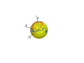
Figure 1: (Color online) Schematic illustration of the traces of FM magnetization vector $\mathbf{m}=\mathbf{M}/M$ and AFM vector $\mathbf{n}=\mathbf{L}/L$ reversal induced by the exposure of PMA-pulses. Small deviation from extremal point $\mathbf{m}=\mathbf{n=}(1,0,0)$ exerts the $\mathbf{m}$ rotation along the track (solid blue curve) close to equatorial $x-y$ plane delineated by dot-dashed circle on Bloch sphere. After PMA $\pi-$pulse terminating the $\mathbf{m}$ relaxes in the direction of reversal state $(-1,0,0)$ (dashed blue line). Much shorter PMA pulse exerts the $\mathbf{n}-$ relaxation into zenith direction (solid red line), which is passed along-track direction due to accumulated velocity. After PMA attenuates the $\mathbf{n}$ continues to relax into reversal state along easy axis (dashed red line).

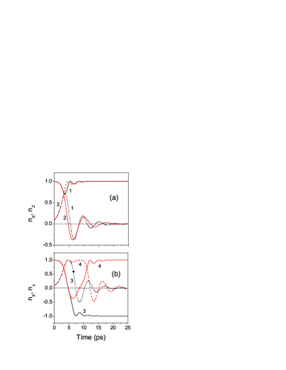
Figure 2: (Color online) The evolution of $x-$ and $z-$ components of AFM vector $\mathbf{n=L/}L$ under PMA pulses of (a) short $\Delta t=3$ ps (curves 1) and long $\Delta t=25$ ps (curves 2) durations. (b) The $\mathbf{n}$ response on intermediate PMA pulse durations $\Delta t=6$ ps (curves 3) and $\Delta t=9$ ps (curves 4). Solid (dashed) lines represent $n_{x}(t)$ [$n_{z}(t)$]. The $n_{y}(t)$ changes insufficiently because of hard $y-$ axis and is not shown. Calculations were carried out in terms of Eqs. ( 5) and (6) for parameters listed in the main text.

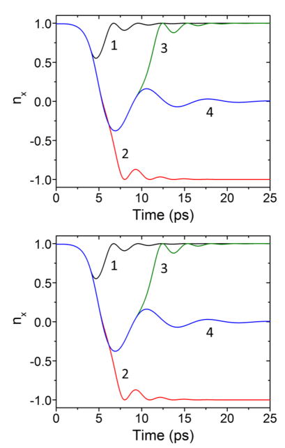
Figure 3: (Color online) Comparison of the Néel vector dynamics obtained with (a) the micro-magnetic simulations and (b) the monodomain approach. The durations 3 ps (curve 1), 5 ps (curve 2), 9 ps (curve 3) and 25 ps (curve 4) of PMA-pulses represent the qualitatively different responses of AFM vector in both approaches. The material parameters are discussed in the main text.

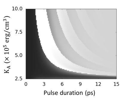
Figure 4: The target states of Néel vector of easy-axis AFM at different PMA pulse duration and its strength. The darker and lighter region represent the starting (initial) state with $n_{x}=1$ and reversal state with $n_{x}=-1$ respectively. The darkness is weighted by the total magnetic energy damping with damping coefficient $\alpha=0.01$. The higher contrast region would have higher probability of deterministic switching, while the lower contrast region (top right) would be vulnerable to thermal noise.

References

- (1) M. N. Baibich, J. M. Broto, A. Fert, F. Nguyen Van Dau, and F. Petroff, P. Eitenne, G. Creuzet, A. Friederich, and J. Chazelas, Phys. Rev. Lett. 61, 2472 (1988).
- (2) S. S. P. Parkin, N. More, and K. P. Roche, Phys. Rev. Lett. 64, 2304 (1990).
- (3) E. V. Gomonay and V. M. Loktev, Low Temp. Phys. 40, 17 (2014).
- (4) R. Cheng, M. W. Daniels, J.-G. Zhu, and D. Xiao, Phys. Rev. B 91, 064423 (2015).
- (5) T. Jungwirth, X. Marti, P. Wadley and J. Wunderlich, Nature Nano., 11, 231 (2016).
- (6) A. S. Núñez, R. A. Duine, P. Haney, and A. H. MacDonald, Phys. Rev. B 73, 214426 (2006).
- (7) E. V. Gomonay and V. M. Loktev, Phys. Rev. B 81, 144427 (2010).
- (8) J. C. Slonczewski, J. Magn. Magn. Mater. 159, L1 (1996).
- (9) C. A. F. Vaz, J. Phys.: Condens. Matter 24, 333201 (2012).
- (10) Y. Hibino, T. Koyama, A. Obinata, K. Miwa, S. Ono, and D. Chiba, Appl. Phys. Express 8, 113002 (2015).
- (11) K. Roy, S. Bandyopadhyay, and J. Atulasimha, Appl. Phys. Lett. 99, 063108 (2011).
- (12) Y. G. Semenov, X. Duan, and K. W. Kim, Phys. Rev. B 86, 161406(R) (2012).
- (13) A. Abragam, The principles of nuclear magnetism, Chapt. 3, Oxford at the Clarendon Press (1961).
- (14) X. Li, D. Carka, C. Liang, A. E. Sepulveda, S. M. Keller, P. K. Amiri, G. P. Carman, and C. S. Lynch, J. Appl. Phys. 118, 014101 (2015).
- (15) C. Grezes, F. Ebrahimi, J. G. Alzate, X. Cai, J. A. Katine, J. Langer, B. Ocker, P. Khalili Amiri, and K. L. Wang, Appl. Phys. Lett. 108, 012403 (2016).
- (16) D. V. Berkov, IEEE Trans. Magn. 38, 2489 (2002).
- (17) V. G. Bar’yakhtar and B. A. Ivanov, Sov. J. Low. Temp. Phys. 5, 361 (1979).
- (18) A. F. Andreev and V. I. Marchenko, Sov. Phys. Usp. 23, 21 (1980).
- (19) I. V. Bar’yakhtar and B. A. Ivanov, Solid State Commun. 34, 545 (1980).
- (20) O. Gomonay, S. Kondovych, and V. Loktev, J. Magn. Magn. Mater. 354, 125 (2014).
- (21) I. Cimrák, Arch. Comput. Methods Eng. 15, 277 (2008).
- (22) X. Duan, Y. G. Semenov, and K. W. Kim, Phys. Rev. Applied 2, 044003 (2014).
- (23) K. Galatsis, K. Wang, Y. Botros, Y. Yang, Y.-H. Xie, J. F. Stoddart, R. B. Kaner, C. Ozkan, J. Liu, M. Ozkan, C. Zhou, and K. W. Kim, IEEE Circuits Devices Mag. 22, 12 (2006).