Efficient inference for genetic association studies with multiple outcomes
Abstract
Combined inference for heterogeneous high-dimensional data is critical in modern biology, where clinical and various kinds of molecular data may be available from a single study. Classical genetic association studies regress a single clinical outcome on many genetic variants one by one, but there is an increasing demand for joint analysis of many molecular outcomes and genetic variants in order to unravel functional interactions. Unfortunately, most existing approaches to joint modelling are either too simplistic to be powerful or are impracticable for computational reasons. Inspired by Richardson et al. (2010, Bayesian Statistics 9), we consider a sparse multivariate regression model that allows simultaneous selection of predictors and associated responses. As Markov chain Monte Carlo (MCMC) inference on such models can be prohibitively slow when the number of genetic variants exceeds a few thousand, we propose a variational inference approach which produces posterior information very close to that of MCMC inference, at a much reduced computational cost. Extensive numerical experiments show that our approach outperforms popular variable selection methods and tailored Bayesian procedures, dealing within hours with problems involving hundreds of thousands of genetic variants and tens to hundreds of clinical or molecular outcomes.
Key words: High-dimensional data; Molecular quantitative trait locus analysis; Sparse multivariate regression; Statistical genetics; Variable selection; Variational inference.
1 Introduction
Much current research in genetics focuses on combining heterogeneous data for the same samples. This is prompted by the increasing availability of diverse molecular data types from a single study and should lead to a more complete understanding of biological systems, as combined inference for data from different molecular layers might unravel regulatory interactions within and across layers (Civelek and Lusis, 2014). An example is protein quantitative trait locus (pQTL) analyses to detect associations between hundreds of thousands of genetic variants and hundreds of proteomic expression levels. When associated with disease genetic variants, proteins are often regarded as intermediate phenotypes or molecular proxies for the disease of interest, as they may provide direct insights on biological processes underlying the clinical condition, and likewise for other molecules such as genes or metabolites involved in so-called eQTL or mQTL analyses.
An important goal of molecular QTL studies is to detect genetic variants with pleiotropic effects, i.e., variants that regulate the expression levels of several molecules, as the genome location where they lie may initiate essential functional mechanisms (Breitling et al., 2008). As pleiotropy has been acknowledged as a central property of genetic variants causing phenotypic variation, efforts are being made to uncover its activity patterns and gain understanding of the shared biological processes it induces (Sivakumaran et al., 2011; Solovieff et al., 2013). It is also of interest to identify those cases where the same molecule is simultaneously influenced by several genetic variants. This dual task requires a model that allows flexible selection, ideally performed jointly on the genetic variants and the molecular outcomes.
Although in practice univariate analyses still dominate, several proposals for joint modelling of multiple outcomes in genetic association problems have recently been made. Flutre et al. (2013) and Zhou and Stephens (2014) model the outcomes as multivariate responses having a matrix-variate distribution. The former rely on a Bayes factor framework to uncover the associations between a given genetic variant and any subset of outcomes, whereas the latter propose a linear mixed model whose random effect accounts for relatedness among individuals. While these methods show improvements over the fully marginal regression approach, they are restricted to problems with a few outcomes, because their models involve unstructured covariance matrices. O’Reilly et al. (2012)’s MultiPhen method reverses the classical regression setup and fits a succession of models where each genetic variant is regressed on several outcomes. This eliminates the need to model large covariance matrices, but also entails a marginal treatment of the genetic variants. Moreover, MultiPhen does not penalize model complexity, which may cause instabilities when many outcomes are modelled. Molecular QTL problems are particularly complex, because in addition to the so-called paradigm, whereby the number of covariates (genetic variants) greatly exceeds the number of samples , there is also a “large ” characteristic, as the number of responses (expression levels) is usually large. Methodologies to accommodate this are needed, especially when joint response modelling is sought.
Two-stage procedures are natural approaches to association problems with both and large. 2HiGWAS (Jiang et al., 2015) is essentially an implementation of the screening strategy of Fan and Lv (2008) in the context of longitudinal outcomes. It consists of a dimension reduction step, where each genetic variant is tested against each outcome, followed by a penalized regression recast into functional mapping in which only the genetic variants remaining after screening are involved. While the second stage of 2HiGWAS is an interesting approach to joint covariate and response modelling, the method is not tailored to typical molecular QTL analysis, as it is designed for outcomes measured over time. Also, the fully marginal first stage screening, if too stringent, may cause important predictors to drop out of the analysis and thus lead to false negatives. Instead of pruning the covariate set, Wang et al. (2016) summarize information at outcome level in the context of eQTL analyses. They precluster the expression levels using a block-mixture model and test for association between each genetic variant and the resulting clustering. This approach requires that the stability of the clustering and its functional relevance are carefully checked, as the group pattern chosen is critical to subsequent analysis. More generally, two-stage procedures often rely on ad-hoc thresholding decisions at the first stage which influence the conclusions of the second stage.
The approaches sketched above use very diverse strategies to model predictor and outcome variables in high-dimensional settings. Trade-offs between realistic modelling and computational efficiency are inevitable, but two components seem critical to practical and powerful analyses: involving all variables in a single multivariate model, and maintaining interpretable inference. Unified selection of genetic variants and associated outcomes is then possible, unlike for most existing methods, whose focus is on selecting either predictors or outcomes. The Bayesian framework seems particularly suitable, as it offers flexible modelling possibilities in which biological beliefs may be naturally incorporated. The hierarchical regression approach of Richardson et al. (2010), HESS (hierarchical evolutionary stochastic search), is an appealing example of such approaches; it can identify associations between hundreds of covariates and up to a few thousand responses from a single model. Jia and Xu (2007) and Scott-Boyer et al. (2012) propose methods called BAYES and iBMQ (integrated Bayesian hierarchical model for eQTL mapping) based on models similar to that of HESS, but a major drawback of all three approaches is the lack of scalability of their Markov chain Monte Carlo inference procedures. Problems whose size corresponds to actual genome-wide association studies with molecular outcomes (with hundreds of thousands of genetic variants and hundreds to thousands of outcomes and individuals) are out of reach even for HESS, which is based on adaptive parallel tempering/evolutionary Monte Carlo techniques. We are unaware of any fully multivariate approach that can deal with such data within a reasonable time.
In this paper, we propose a Bayesian inference strategy that avoids sampling, via an algorithm that is fast and whose convergence is easy to monitor, while having performance comparable with Markov chain Monte Carlo approaches. We describe a variational inference procedure for a model similar to that of Richardson et al. (2010), comprising a series of parallel linear regressions, one for each response, combined in a hierarchical manner to leverage shared information. A spike-and-slab prior (Ishwaran and Rao, 2005) is used to induce sparsity of the regression coefficients, and the probability that a given covariate affects any response is modelled through a parameter that is shared across responses. Interpretable posterior quantities, such as the probability of association of each covariate-response pair, are produced. An efficient algorithm for this model is crucial, as its number of parameters can be very large. Our variational approach can update the parameters jointly in a tractable manner. Carbonetto and Stephens (2012) provide a good discussion of variational inference in the context of genetic association and propose a variational regression method called “varbvs”, which can be seen as a single-response counterpart of our approach. In our multiple response setting, we show by simulation that our procedure is accurate and reliable, and is better than existing methods at selecting variables for very large problems. Hence, it offers clear added-value in practice: it enables complex and flexible Bayesian inference based on large batches of genetic data, without having to prune them beforehand.
The paper is organized as follows. Section 2 describes the model, discusses its relation to earlier proposals, and presents a procedure to allow for sparsity control at both covariate and response levels. Section 3 gives an overview of variational Bayes approaches and describes our inference strategy. Section 4 compares variational and Markov chain Monte Carlo inferences on the same model, also using direct approximations of posterior quantities. Section 5 describes numerical experiments for larger problems, comparing our method with several predictor selection methods, including the varbvs approach of Carbonetto and Stephens (2012), and with methods performing combined covariate and response selection, namely HESS (Richardson et al., 2010) and iBMQ (Scott-Boyer et al., 2012). The section also presents a permutation-based comparison of our method with varbvs on a real mQTL problem. Section 6 summarizes the discussion and highlights further possible developments.
Although the applicability of our method is not restricted to any particular context, all the numerical experiments presented in this paper use settings tailored to genome-wide association studies. The data-generation schemes are designed to embody common biological assumptions and are described in Section 5.1. The method is implemented in the publicly available R package locus.
2 Model and earlier proposals
Let be a matrix of centered responses and let be a matrix of covariates, for each of samples. The covariates are genetic variants, more precisely single nucleotide polymorphisms, SNPs, and the responses might represent gene, protein or metabolite expression levels for individuals, depending on whether an eQTL, pQTL or mQTL problem is considered. Our model is intended to accommodate all the constraints entailed by molecular QTL analyses; it is adapted from that of HESS (Richardson et al., 2010). Suppose that
where is the Dirac distribution. Each response, , is related linearly to the covariates and has a specific precision, . The responses are conditionally independent across the regressions, but dependence among responses associated with the same covariates is captured through the prior specification of parameters and , which are shared across the responses. This formulation circumvents modelling the covariance between the responses, which is infeasible when is large. Each covariate-response pair has its own regression parameter, , for which sparsity is induced using a spike-and-slab prior. The binary parameter acts as a “pair selection” indicator; covariate is associated with response if and only if . The parameter represents the typical size of nonzero effects and is modulated by the residual variance, , of the response concerned by the effect. The parameters specify the response(s) associated with and are identically distributed as Bernoulli with common parameter . Thus, controls the proportion of responses associated with covariate . The goal of inference is variable selection. Selection of predictors can be performed by ranking the posterior means of and selection of covariate-response pairs can be performed by ranking the posterior probabilities of inclusion, i.e., the posterior means of .
Our model differs from that of Richardson et al. (2010) in two respects. One concerns the treatment of the regression coefficient parameters : we use independent priors, whereas Richardson et al. rely on g-priors (Zellner, 1986). The main motivation for our choice is that the effects of genetic variants on a given outcome can be understood as causal, since no retroactive process can affect the variants, and they can take place at locations of the genome that are far apart, so their correlation structure need not reflect the spatial correlation of the SNPs; see Guan and Stephens (2011). Jia and Xu (2007) also rely on independent priors for the regression coefficients of BAYES, but they model the latter with a mixture of two normal distributions rather than a spike-and-slab prior and impose a residual variance parameter that is common to all responses. This stringent assumption may represent a weakness of their proposal.
The second difference concerns the third level of the model. Richardson et al. (2010) opt for a quite complex specification, in which
| (1) |
In their case, the inclusion probability of for response is modelled through ; it is specific to that response but can be regulated using the parameter , common to all responses. Jia and Xu (2007) and Scott-Boyer et al. (2012) propose other variants for this prior. The former choose a treatment similar to ours, with , and the latter consider an additional level of hierarchy,
| (2) |
with and . Our choice is partly driven by our wish to design a simpler model and partly by practical considerations, since it ensures a closed form for our variational algorithm, unlike with (1). While such a formulation was mentioned by Richardson et al. (2010) and by Scott-Boyer et al. (2012), they did not pursue it because of concerns regarding its ability to control for multiplicity. Indeed, our model inherently enforces sparse associations as the number of responses, , increases, but no control is achieved when the number of covariates, , grows. We address this below by providing a procedure to induce a correction through the prior of .
Part of the flexibility of our model comes from the fact that the hyperparameters, , (for ’s Beta prior), , (for ’s Gamma prior) and , (for ’s Gamma prior) are readily interpreted. One option is to set them based on external information regarding the likelihood of given associations, if available. For instance, to favour associations with covariate , one can set and so that the prior proportion of responses affected by , , is large. The use of such assumptions may be very efficient, but it may also skew the inference towards existing knowledge. In the simulations presented in this paper, we assume that the regression and variance parameters are exchangeable, i.e., that all covariates, and responses have the same prior propensity to be involved in associations, by selecting a single value for all components of , , and . Without favouring any covariate or response, however, we can control signal sparsity at the level of covariates by specifying (possibly through cross-validation) a prior average number of covariates, , expected to be included in the model. Setting
| (3) |
the prior probability that is associated with at least one response is
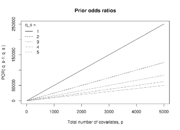
and simpler models are favoured as increases. To see this, one can consider the prior odds ratio representing the support for a model to have an additional response associated with , i.e.,
| (4) |
Clearly, penalties arise and increase with the total number of responses in the model, . Figure 1 displays for as a function of and indicates that, when and are specified as in , the penalties also increase with the total number of covariates, , therefore naturally adjusting for multiplicity. Moreover, the penalties are not uniform when moving from one to two responses associated with , or from four to five, for instance.
The experiment reported in Table 1 confirms that adjustment takes place in practice. It considers problems with “active” covariates, i.e., those associated with at least one response, and an increasing number of “noise” covariates and it compares the regime with and set according to (3) to an “uncorrected” regime with , , so that the prior mean number of responses associated with is , i.e., . The number of false positives, based on a posterior probability of inclusion greater than , grows linearly with when the uncorrected model is used but remains roughly constant close to zero with correction (3), giving a clear multiplicity adjustment. Other experiments confirmed strong sparsity control; the reported findings on real data should therefore be plausible when (3) is used.
| Mean # of FP | |||||
|---|---|---|---|---|---|
| Uncorrected | () | () | () | () | () |
| Corrected | () | () | () | () | () |
| Mean # of TP | |||||
| Uncorrected | () | () | () | () | () |
| Corrected | () | () | () | () | () |
3 Variational inference
Section 2 described some differences between our model and those of Jia and Xu (2007, BAYES), Richardson et al. (2010, HESS) and Scott and Berger (2010, iBMQ), but a more fundamental distinction concerns the inference procedure. The three earlier methods rely on Markov chain Monte Carlo (MCMC) techniques and require massive computing resources when the dimensionality of the problem is large. We instead employ a variational inference procedure, which is deterministic and hence can be much cheaper (Ormerod and Wand, 2010).
Instead of sampling from the joint posterior probability of the parameter vector of interest, , variational approaches proceed by replacing it by a tractable analytical approximation, . We focus on so-called mean-field variational formulations (Xing et al., 2002; Attias, 2000) to construct such a class, i.e., we assume that factorizes over some partition of , ,
no further assumption is made about the distribution, and in particular no constraint is imposed on the functional forms of the . Here, we consider the factorization
| (5) |
and turn the inference into an optimization problem where is obtained by minimizing its Kullback–Leibler divergence from the target distribution, . Because the marginal log-likelihood may be written as
| (6) |
where
minimizing the Kullback–Leibler divergence amounts to maximizing , which represents a lower bound for . To this end, we observe that
| (7) | |||||
where cst is constant with respect to and where we introduced the distribution
with denoting the expectation with respect to the distributions over all variables , . The right-hand side of (7) corresponds to the negative Kullback–Leibler divergence between and , plus a constant. Hence, assuming that the , , are fixed, the distribution which maximizes is , i.e., the maximum of occurs when
| (8) |
The relations give rise to cyclic dependencies among the densities . This suggests an iterative algorithm whose convergence can easily be monitored by evaluating changes in the lower bound . Our choice (5) ensures that the coordinate updates can be derived in closed form; in particular, the semi-conjugacy of our model implies that the prior densities of all parameters are preserved by the variational densities. For instance, a spike-and-slab distribution with modified parameters is recovered at posterior level, with
where the variational parameters , , are to be updated iteratively. Convergence is ensured by the convexity of in each of the (Boyd and Vandenberghe, 2004, §§ 3.1.5, 3.2.4, 3.2.5). The algorithm and its derivation are given in Appendix B.
4 Empirical quality assessment of the variational approximation
4.1 Tightness of the marginal log-likelihood lower bound
In this section we evaluate the closeness of the variational density to the target posterior distribution by approximating the Kullback–Leibler divergence . Because of relation , this amounts to assessing the tightness of the variational lower bound for the marginal log-likelihood, . For small problems, the likelihood may be accurately approximated using simple Monte Carlo sums. We have
with
where
see Appendix C for details. As no closed form is available for the remaining integrals, we use
where we independently generate
| (9) |
Figure 2 displays the relative difference for problems with covariates, responses and increasing sample sizes, . In the left panel, the covariates are independent of each other, and so are the responses. In the right panel, the covariates are equicorrelated with correlation coefficient , and so are the responses. In both cases, the mean relative difference is below with and seems to decrease as grows. Although we are not aware of any such study with which to benchmark our results, these values seem very small, suggesting that our variational distribution adequately reflects the target distribution , at least for small problems. Likewise, the variational lower bound may be used as a proxy for the marginal log-likelihood when performing model selection; this use will be illustrated in Section 5.3. The fact that the variational lower bound remains tight in the correlated data case is reassuring, as it suggests that the independence assumptions underlying the mean-field factorization of may only weakly impact the quality of the approximation.


4.2 Comparison with Markov Chain Monte Carlo
| Active | Inactive | |||||
| (avg) | ||||||
| Truth | ||||||
| VB | () | () | () | () | () | () |
| MCMC | () | () | () | () | () | () |
| Active | Inactive | |||||
| (avg) | ||||||
| True prop. of active resp. | ||||||
| VB | () | () | () | () | () | |
| MCMC | () | () | () | () | () | |
| Simple Monte Carlo |
We complement our quality assessment by comparing several variational posterior quantities with those for MCMC inference on problems of moderate size. A fair comparison is not straightforward, as these two types of inference rely on stopping rules and convergence diagnostics of very different natures. While the convergence criterion for variational inference comes down to a tolerance to be prescribed, the ability of MCMC sampling to adequately explore the model space for a given chain length can be difficult to evaluate, and usually varies greatly with the problem size. To alleviate the risk of inaccurate MCMC inference, we run iterations and discard the first half. We also support our comparison with selected quantities approximated by simple Monte Carlo sums, namely, the posterior probability of inclusion of a covariate for a response ,
and the posterior mean of , controlling the proportion of responses associated with covariate ,
with the samples and generated as in , with draws.
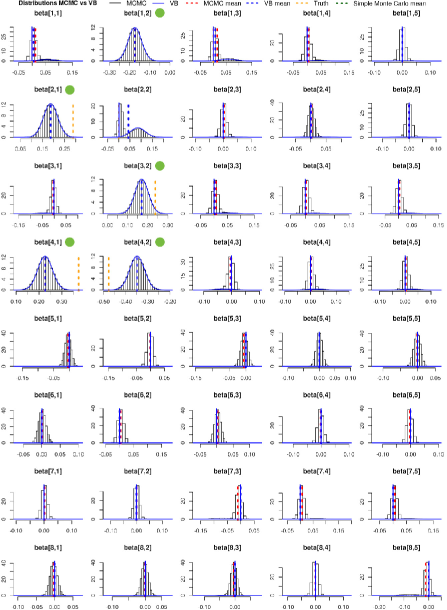
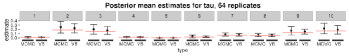
Table 2 reports the variational, MCMC and simple Monte Carlo estimates of and for a problem with covariates, responses for samples, and with each nonzero association explaining on average of response variance. The estimates all agree closely. Those of the five active regression coefficients, , , , and , are significantly different from zero, unlike the average estimate of the inactive coefficients. A plot of the MCMC and variational posterior densities (the latter obtained in closed form), given in Figure 7 of Appendix C.2, shows that the posterior modes of the inactive coefficients are all zero. Moreover, in this case the variational distributions are usually solely made up of a clear spike at zero, whereas the MCMC histograms correspond roughly to a centered Gaussian distribution with average standard deviation . Table 2 also indicates a shrinkage effect for both variational and MCMC posterior means of the nonzero compared to the true values. This is a consequence of the spike-and-slab prior but does not seem to hamper the detection of the association signals, since the posterior probabilities of inclusion of the true nonzero associations are concentrated around , while those corresponding to noise are usually much lower, whether obtained by MCMC, variational or simple Monte Carlo procedures; see Figure 8 of Appendix C.2. Finally, the estimates of in Table 2 provide a fair approximation to the actual proportion of responses associated with a given covariate.
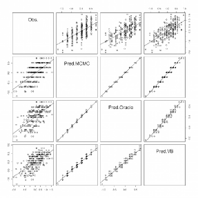
Two additional numerical experiments comparing variational and MCMC posterior quantities are provided in Appendix C.2. One compares the estimates of and with the true values when the data are generated from the model with covariates and responses. It also provides receiver operating characteristic (ROC) curves assessing the pairwise variable selection performance for both inference types. The other simulation gathers the observed values, , and the estimated posterior means of obtained by variational and MCMC procedures and an oracle. Both experiments indicate equivalent performance for MCMC and variational inferences.
5 Statistical performance
5.1 Predictor selection
The problems considered in Section 4.2 were small enough to allow accurate and tractable MCMC inference. In this section, we assess the performance of our approach on larger problems by comparing it to popular variable selection methods; i.e., with joint modelling of outcomes and covariates (elastic net for multivariate Gaussian responses), with joint modelling of covariates only (Bayesian multiple regression based on MCMC inference, “BAS”, or variational inference, “varbvs”), or with fully marginal modelling (univariate ordinary least squares and “lmBF” Bayesian regressions). Complete descriptions and references are in Appendix D.2. The methods are compared by measuring their ability to detect the active covariates, i.e., to determine which covariates are associated with at least one response. For our variational approach, this task is achieved by ranking the posterior means of the , which control the proportion of responses associated with a given covariate.
Our data-generation design is based on generally accepted principles of population genetics. We simulate SNPs under Hardy–Weinberg equilibrium from a binomial distribution with probabilities corresponding to minor allele frequencies of common variants, chosen in the interval uniformly at random, and we generate outcomes from Gaussian distributions with specific error variances. The dependence structure of these variables is either enforced block-wise with preselected auto- or equicorrelation coefficients or chosen to be that of real data. The labels of the active SNPs and outcomes are picked randomly, and each active SNP is associated to one (randomly selected) active outcome and to each of the remaining active outcomes with a prescribed probability; some outcomes are therefore under pleiotropic control. The proportions of outcome variance explained per SNP are simulated for all associations from a positively skewed Beta distribution to favour the generation of smaller effects, and they are then rescaled to match a given average proportion. To mimic the result of natural selection, the effect sizes are inversely related to the SNP minor allele frequencies. For more details, see Appendix D.1.
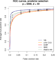
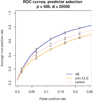

We perform replications for each of three simulation configurations. The first configuration has moderate numbers of covariates () and outcomes (), and allows time-consuming methods to run within hours. The second has many outcomes () and the third has many covariates (); these numbers approach those encountered in molecular QTL studies. The remaining settings (numbers of active outcomes and covariates, of observations, effect sizes, etc) are detailed in the caption to Figure 3.
The ROC curves in Figure 3 indicate that our approach outperforms the other methods. It is appreciably more powerful for low false positive rates, which are of particular interest for the highly sparse scenarios typically expected for genome-wide association studies. Despite the correlation among the covariates and the outcomes, our method does not seem to suffer from the independence assumptions implied by the mean-field approximation, as suggested by the results of Section 4.1. The marginal ordinary least squares and marginal lmBF regressions appear to miss many associations because of their univariate modelling of covariates, but jointly accounting for the covariates may not suffice, as suggested by the rather poor performances of the Bayesian multiple regression approaches, BAS and varbvs, which apply separate multiple linear regressions for each outcome. It appears that the ability of our approach to exploit the similarity across outcomes yields more power to detect their shared associations. Finally, even though the multivariate elastic net models jointly the covariate and outcome variables, its inference suffers from the assumption that to each covariate corresponds a single regression coefficient, shared for all responses. As a consequence, regression estimates of covariates with weak or few associations with the responses may be shrunk to zero.
5.2 Combined selection of predictors and outcomes


Unlike the classical variable selection methods used as comparators in Section 5.1, our approach and those of Richardson et al. (2010), HESS, and Scott-Boyer et al. (2012), iBMQ, are tailored to molecular QTL problems: they quantify the associations between each covariate-response pair in a single model, and thus provide flexible and unified frameworks for detecting pairs of associated SNP-molecules, as well as pleiotropic SNPs associated with many molecular outcomes. In this section, we compare the three approaches in terms of the posterior quantities used to perform such selection. As both HESS and iBMQ rely on MCMC sampling, we consider smaller problems than in Section 5.1 in order to ensure convergence within a reasonable time. The simulated datasets have covariates, of which are active, and outcomes, of which are active, the probability of association being , for samples. On average, the active covariates account for of the variance of an outcome with which they are associated. HESS was run with three MCMC chains, the number selected by the authors for their simulations but with iterations of which were discarded as burn-in. For iBMQ, iterations were saved after removal of burn-in samples, as suggested in the package documentation for a problem of comparable dimensions. Inference for one replication took on average seconds with our method, around minutes with iBMQ and hours with HESS (GPU computation option disabled, since no GPU was available to us) on an Intel Xeon CPU at 2.60 GHz with 64 GB RAM.
| TPR | TNR | |
|---|---|---|
| VB | () | () |
| HESS | () | () |
| iBMQ | () | () |
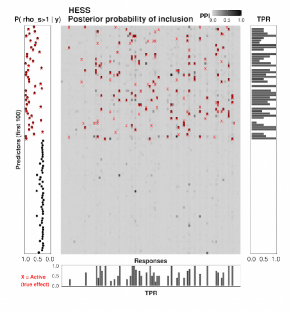
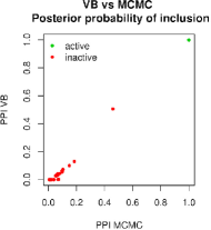
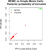
Figure 4 compares the marginal posterior probabilities of inclusion obtained by our method with those of HESS and iBMQ. We observe a strong correlation between our approach and HESS, with a quite good ability to discriminate between active and inactive covariate-response pairs. There is a discrepancy at the zero ordinate, where HESS signals a series of false positives and few true positives. The comparison with iBMQ is more contrasted, as the values of its posterior probabilities of inclusion for many true associations are below and indistinguishable from noise. The same conclusions are reached when running the three methods on additional datasets, as suggested by Table 3, which gathers sensitivity and specificity measures based on median probability models (Barbieri and Berger, 2004) (consisting of those covariate-response pairs whose posterior inclusion probability is higher than ). As discussed in Section 2, control of signal sparsity can be induced through the prior for , still, rather than median probability models, one may prefer to use a data-driven false discovery threshold in order to prescribe a desired level of false discoveries.
Figure 5 compares the patterns recovered by HESS and by our method, again based on the marginal posterior probabilities of inclusion from the first replicate. Visual comparison of the true positive rates suggests that the abilities of the two approaches to detect the true associations are very similar. Our approach indicates the presence of associations in the region of active covariates only, whereas the HESS pattern is blurrier in regions of inactive covariates. The posterior means of from our approach discriminate quite well between active and inactive covariates, and so do, for HESS, the posterior probabilities (), described by Richardson et al. (2010) as capturing the propensity for a given covariate to influence several responses simultaneously.

5.3 Application to a real mQTL dataset
We end these numerical experiments by illustrating our approach on data from a large multicenter dietary intervention study called Diogenes (Larsen et al., 2010). The study contains a series of genomic data types collected at different stages of a dietary treatment provided to the cohort. Its goal is to uncover molecular mechanisms underlying the metabolic status of overweight individuals and improve understanding of the factors predisposing weight regain after a diet. Here, we perform a metabolite quantitative trait locus (mQTL) analysis; in this context, the metabolites may be viewed as proxies for the clinical condition of interest, weight maintenance. We also use this illustration on real data to further highlight the benefits of modelling the outcomes jointly via an extensive permutation-based comparison with the single-response variational method varbvs (Carbonetto and Stephens, 2012).
After quality control, the data consist of tag SNPs and metabolite expression levels, adjusted for age, center and gender, for individuals. The SNPs were collected on Illumina HumanCore arrays and the metabolites were quantified in plasma using liquid chromatography-mass spectrometry (LC-MS). They span cholesterol esters (CholE), phosphatidylcholines (PC), phosphatidylethanolamines (PE), sphingomyelins (SM), di- (DG) and triglycerides (TG). Appendix E.1 provides more details.
| # declared: | |||
| Permutation-based FDR (%) | VB | varbvs | VB varbvs |
| 5 | 21 | 19 | 8 |
| 10 | 26 | 19 | 8 |
| 15 | 47 | 21 | 10 |
| 20 | 76 | 31 | 12 |
| 25 | 89 (48 univ.) | 47 (19 univ.) | 14 (13 univ.) |
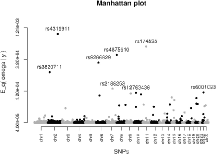

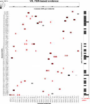
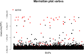
In order to adjust for multiplicity, we specify the hyperparameters for according to the discussion of Section 2 and choose the prior average number of active SNPs, , by grid search within a -fold cross-validation procedure that maximizes the variational lower bound. After hyperparameter selection, the algorithm converged in iterations, taking about hours on an Intel Xeon CPU at 2.60 GHz with 512 GB RAM. The posterior means suggest the presence of several active SNPs, spread across the chromosomes (Figure 6), but we use the marginal posterior inclusion probabilities, , to declare pairwise associations and active SNPs.
We compare varbvs and our method on real data based on the number of associations declared by each method at specific false discovery rates estimated by permutations. We apply Efron’s Bayesian interpretation of the false discovery rate (Efron, 2008) to posterior probabilities of inclusion, and use an empirical null distribution based on permutations to compute the estimate
| (10) |
for a grid of thresholds ; we then fit a cubic spline to the resulting false discovery rates to find thresholds for specific rates. The analysis suggests that our method is more powerful, with associations declared at an estimated FDR of , against for varbvs; the superiority of our method is further highlighted by Table 4. Figure 6 displays the associations declared by our method and the overlap with those declared by varbvs at estimated FDR of ; the associations detected also largely agree with those obtained with marginal screening at Benjamini–Hochberg FDR of .
Database searches on the functional relevance of the detected associations give hints of promising biological functions related to metabolic activities for of the SNPs declared as active by our procedure. For instance, the most outstanding SNP Figure 6, , shows many associations with triglyceride levels, and turns out to be located less than from the protein coding gene ITGA6 known to be linked to diabetic kidney disease (Iyengar et al., 2015). The second most prominent pleiotropic SNP, , is declared by our approach to be associated with phospholipids, more precisely with different phosphatidylcholine levels, of which four are ether-linked/plasmalogen (PC-O). Interestingly, this latter SNP has been recently reported to be related to metabolite levels; among others, it was found to be associated with trans fatty acid levels and plasma phospholipid levels (Mozaffarian et al., 2015), in line with our findings. Moreover, it was found to be an eQTL for the fatty acid desaturase genes FADS1 and FADS2. The SNP too has been identified as associated with very long-chain fatty acid levels (Lemaitre et al., 2015). This seems to agree with our findings, in which exhibits associations with sphingomyelin, a type of lipid containing fatty acids of different chain lengths. The complete subset of SNPs with metabolism-related links found by our procedure is given in Appendix E. Additional details on this real data study, as well as on its replication using simulated data, are also provided there.
6 Conclusions
We have described a scalable and efficient approach to joint variable selection from large numbers of candidate predictor and outcome variables. As it exploits the similarity across outcomes through a flexible hierarchical structure, our procedure outperforms the most popular predictor selection approaches in high-dimensional set-ups. The variational approximation on which our approach relies provides accurate posterior quantities, with reduced computational effort relative to MCMC procedures; in particular, it yields inferences comparable to those of the MCMC procedure HESS (Richardson et al., 2010). Convergence control is automatic, whereas convergence assessment for MCMC algorithms can be difficult, especially in high dimensions. Our simulations also show that variable selection remains powerful when the predictors and outcomes are correlated, notwithstanding the independence assumptions underlying the mean-field factorization.
The key added-value of our approach is its applicability to molecular QTL datasets without the need for prior dimension reduction. In an application, our approach recovered several previously reported SNP-metabolite associations, and declared more associations than the single-outcome method “varbvs” (Carbonetto and Stephens, 2012) at prescribed false discovery rates, thus highlighting the benefits of jointly modelling the outcomes. To the best of our knowledge, no competing Bayesian approach for joint inference on two high-dimensional sets of variables can deal with the problem sizes typically encountered in molecular QTL analyses.
Bioinformatics is moving towards whole-genome analyses, for which several million genetic variants need to be considered, so it seems worthwhile to consider further speed-up strategies for our approach. One option is to use new optimization procedures. So-called natural gradient methods, which rely on the Riemannian structure of variational approximate distributions, seem particularly attractive, as they can be orders of magnitude faster than conventional gradient algorithms (Honkela et al., 2008). Another possibility is a “split-and-merge” strategy, i.e., first partitioning the variable space and then inferring a global variational distribution on the aggregated dataset. Tran et al. (2016) designed a variant of this approach for sample space partitioning. At the recombination step, they proposed to “merge” the variational distributions by exploiting the independence assumptions of the mean-field formulation. Both strategies could lead to significant computational gains.
7 Software
The algorithm and the data-generation functions used in this paper are implemented in the publicly available R package locus.
Acknowledgements
The authors are grateful to the Associate Editor and the two referees for their very helpful comments that improved the paper. We thank Jérôme Carayol, Loris Michel and Armand Valsesia for their valuable comments. We also thank James Holzwarth, Bruce O’Neel and Jaroslaw Szymczak for giving us access to computing resources.
Funding
The Diogenes trial was supported by the European Commission (FP6-2005-513946) and Nestlé Institute of Health Sciences.
References
- Abramowitz and Stegun (1965) M. Abramowitz and I. A. Stegun. Handbook of Mathematical Functions. Dover Publications, Inc., New York, 1965.
- Attias (2000) H. Attias. A variational Bayesian framework for graphical models. Advances in Neural Information Processing Systems, 12:209–215, 2000.
- Barbieri and Berger (2004) M. M. Barbieri and J. O. Berger. Optimal predictive model selection. Annals of Statistics, 32:870–897, 2004.
- Bates and Maechler (2015) D. Bates and M. Maechler. Matrix: Sparse and dense matrix classes and methods, 2015, 2015. R package version 1.2.2.
- Boyd and Vandenberghe (2004) S. Boyd and L. Vandenberghe. Convex Optimization. Cambridge University Press, New York, 2004.
- Breitling et al. (2008) R. Breitling, Y. Li, B. M. Tesson, J. Fu, C. Wu, T. Wiltshire, A. Gerrits, L. V. Bystrykh, G. De Haan, A. I. Su, et al. Genetical genomics: spotlight on QTL hotspots. PLoS Genetics, 4:e1000232, 2008.
- Carbonetto and Stephens (2012) P. Carbonetto and M. Stephens. Scalable variational inference for Bayesian variable selection in regression, and its accuracy in genetic association studies. Bayesian Analysis, 7:73–108, 2012.
- Civelek and Lusis (2014) M. Civelek and A. J. Lusis. Systems genetics approaches to understand complex traits. Nature Reviews Genetics, 15:34–48, 2014.
- Clyde (2016) M. Clyde. BAS: Bayesian Adaptive Sampling for Bayesian Model Averaging, 2016. R package version 1.0.9.
- Efron (2008) B. Efron. Microarrays, empirical Bayes and the two-groups model. Statistical Science, 23:1–22, 2008.
- Fan and Lv (2008) J. Fan and J. Lv. Sure independence screening for ultrahigh dimensional feature space (with Discussion). Journal of the Royal Statistical Society: Series B (Statistical Methodology), 70(5):849–911, 2008.
- Flutre et al. (2013) T. Flutre, X. Wen, J. Pritchard, and M. Stephens. A statistical framework for joint eQTL analysis in multiple tissues. PLoS Genetics, 9:e1003486, 2013.
- Friedman et al. (2009) J. H. Friedman, T. J. Hastie, and R. J. Tibshirani. glmnet: Lasso and elastic-net regularized generalized linear models, 2009. R package version 2.0.2.
- George and McCulloch (1997) E. I. George and R. E. McCulloch. Approaches for Bayesian variable selection. Statistica Sinica, 7:339–373, 1997.
- Guan and Stephens (2011) Y. Guan and M. Stephens. Bayesian variable selection regression for genome-wide association studies and other large-scale problems. Annals of Applied Statistics, 5:1780–1815, 2011.
- Higham (2002) N. J. Higham. Computing the nearest correlation matrix—a problem from finance. IMA Journal of Numerical Analysis, 22:329–343, 2002.
- Honkela et al. (2008) A. Honkela, M. Tornio, T. Raiko, and J. Karhunen. Natural conjugate gradient in variational inference. In M. Ishikawa, Kenji Doya, H. Miyamoto, and T. Yamakawa, editors, Neural Information Processing: 14th International Conference, ICONIP 2007, Kitakyushu, Japan, November 13-16, 2007, Revised Selected Papers, Part II, pages 305–314. Springer, Berlin, 2008.
- Ishwaran and Rao (2005) H. Ishwaran and J. S. Rao. Spike and slab variable selection: frequentist and Bayesian strategies. Annals of Statistics, 33:730–773, 2005.
- Iyengar et al. (2015) S. K. Iyengar, J. R. Sedor, B. I. Freedman, W. L. Kao, M. Kretzler, B. J. Keller, H. E. Abboud, S. G. Adler, L. G. Best, and D. W. Bowden. Genome-wide association and trans-ethnic meta-analysis for advanced diabetic kidney disease: family investigation of nephropathy and diabetes (FIND). PLoS Genetics, 11:e1005352, 2015.
- Jia and Xu (2007) Z. Jia and S. Xu. Mapping quantitative trait loci for expression abundance. Genetics, 176:611–623, 2007.
- Jiang et al. (2015) L. Jiang, J. Liu, X. Zhu, M. Ye, L. Sun, X. Lacaze, and R. Wu. 2HiGWAS: a unifying high-dimensional platform to infer the global genetic architecture of trait development. Briefings in Bioinformatics, 16:bbv002, 2015.
- Karolchik et al. (2003) D. Karolchik, R. Baertsch, M. Diekhans, T. S. Furey, A. Hinrichs, Y. T. Lu, K. M. Roskin, M. Schwartz, C. W. Sugnet, and D. J. Thomas. The UCSC genome browser database. Nucleic Acids Research, 31:51–54, 2003.
- Larsen et al. (2010) T. M. Larsen, S.-M. Dalskov, M. van Baak, S. A. Jebb, A. Kafatos, A. F. H. Pfeiffer, J. A. Martinez, T. Handjieva-Darlenska, M. Kunesova, C. Holst, W. H. M. Saris, and A. Astrup. The Diet, Obesity and Genes (Diogenes) Dietary study in eight European countries—a comprehensive design for long-term intervention. Obesity Reviews, 11:76–91, 2010.
- Lemaitre et al. (2015) R. N. Lemaitre, I. B. King, E. K. Kabagambe, J. H. Y. Wu, B. McKnight, A. Manichaikul, W. Guan, Q. Sun, D. I. Chasman, and M. Foy. Genetic loci associated with circulating levels of very long-chain saturated fatty acids. Journal of Lipid Research, 56:176–184, 2015.
- Lonsdale et al. (2013) J. Lonsdale, J. Thomas, M. Salvatore, R. Phillips, E. Lo, S. Shad, R. Hasz, G. Walters, F. Garcia, and N. Young. The genotype-tissue expression (GTEx) project. Nature Genetics, 45:580–585, 2013.
- Morey and Rouder (2015) R. D. Morey and J. N. Rouder. BayesFactor: computation of Bayes factors for common designs, 2015. R package version 0.9.12-2.
- Mozaffarian et al. (2015) D. Mozaffarian, E. K. Kabagambe, C. O. Johnson, R. N. Lemaitre, A. Manichaikul, Q. Sun, M. Foy, L. Wang, H. Wiener, and M. R. Irvin. Genetic loci associated with circulating phospholipid trans fatty acids: a meta-analysis of genome-wide association studies from the CHARGE Consortium. The American Journal of Clinical Nutrition, 101:398–406, 2015.
- O’Reilly et al. (2012) P. F. O’Reilly, C. J. Hoggart, Y. Pomyen, F. C. F. Calboli, P. Elliott, M.-R. Jarvelin, and L. J. Coin. MultiPhen: joint model of multiple phenotypes can increase discovery in GWAS. PLoS One, 7:e34861, 2012.
- Ormerod and Wand (2010) J. T. Ormerod and M. P. Wand. Explaining variational approximations. The American Statistician, 64:140–153, 2010.
- Park et al. (2011) J.-H. Park, M. H. Gail, C. R. Weinberg, R. J. Carroll, C. C. Chung, Z. Wang, S. J. Chanock, J. F. Fraumeni, and N. Chatterjee. Distribution of allele frequencies and effect sizes and their interrelationships for common genetic susceptibility variants. Proceedings of the National Academy of Sciences, 108:18026–18031, 2011.
- Plummer et al. (2006) M. Plummer, N. Best, K. Cowles, and K. Vines. CODA: Convergence Diagnosis and Output Analysis for MCMC, 2006. R package version 0.18.1.
- Rebhan et al. (1998) M. Rebhan, V. Chalifa-Caspi, J. Prilusky, and D. Lancet. GeneCards: a novel functional genomics compendium with automated data mining and query reformulation support. Bioinformatics, 14:656–664, 1998.
- Richardson et al. (2010) S. Richardson, L. Bottolo, and J. S. Rosenthal. Bayesian models for sparse regression analysis of high-dimensional data. In J. M. Bernardo, M. J. Bayarri, J. O. Berger, A. P. Dawid, D. Heckerman, A. F. M. Smith, and M. West, editors, Bayesian Statistics, volume 9, pages 539–569. Oxford University Press, New York, 2010.
- Scott and Berger (2010) J. G. Scott and J. O. Berger. Bayes and empirical-Bayes multiplicity adjustment in the variable-selection problem. Annals of Statistics, 38:2587–2619, 2010.
- Scott-Boyer et al. (2012) M. P. Scott-Boyer, G. C. Imholte, A. Tayeb, A. Labbe, C. F. Deschepper, and R. Gottardo. An integrated hierarchical Bayesian model for multivariate eQTL mapping. Statistical Applications in Genetics and Molecular Biology, 11:1515–1544, 2012.
- Sivakumaran et al. (2011) S. Sivakumaran, F. Agakov, E. Theodoratou, J. G. Prendergast, L. Zgaga, T. Manolio, I. Rudan, P. McKeigue, J. F. Wilson, and H. Campbell. Abundant pleiotropy in human complex diseases and traits. The American Journal of Human Genetics, 89:607–618, 2011.
- Solovieff et al. (2013) N. Solovieff, C. Cotsapas, P. H. Lee, S. M. Purcell, and J. W. Smoller. Pleiotropy in complex traits: challenges and strategies. Nature Reviews Genetics, 14:483–495, 2013.
- Spiegelhalter et al. (2007) D. Spiegelhalter, A. Thomas, N. Best, and D. Lunn. OpenBUGS user manual, version 3.0. 2, 2007. MRC Biostatistics Unit, Cambridge.
- Tran et al. (2016) M.-N. Tran, D. J. Nott, A. Y. C. Kuk, and R. Kohn. Parallel variational Bayes for large datasets with an application to generalized linear mixed models. Journal of Computational and Graphical Statistics, 25:626–646, 2016.
- Tukey (1949) J. W. Tukey. Comparing individual means in the analysis of variance. Biometrics, 5:99–114, 1949.
- Wang et al. (2016) N. Wang, K. Gosik, R. Li, B. Lindsay, and R. Wu. A block mixture model to map eQTLs for gene clustering and networking. Scientific Reports, 6:21193, 2016.
- Welter et al. (2014) D. Welter, J. MacArthur, J. Morales, T. Burdett, P. Hall, H. Junkins, A. Klemm, P. Flicek, T. Manolio, and L. Hindorff. The NHGRI GWAS Catalog, a curated resource of SNP-trait associations. Nucleic Acids Research, 42:D1001–D1006, 2014.
- Xing et al. (2002) E. P. Xing, M. I. Jordan, and S. Russell. A generalized mean-field algorithm for variational inference in exponential families. In Proceedings of the Nineteenth Conference on Uncertainty in Artificial Intelligence, pages 583–591, San Francisco, 2002. Morgan Kaufmann.
- Zellner (1986) A. Zellner. On assessing prior distributions and Bayesian regression analysis with g-prior distributions. In Studies in Bayesian Econometrics, volume 6, pages 233–243. Elsevier, New York, 1986. P. K. Goel and A. Zellner, editors.
- Zhou and Stephens (2014) X. Zhou and M. Stephens. Efficient algorithms for multivariate linear mixed models in genome-wide association studies. Nature Methods, 11:407, 2014.
Appendix A Multiplicity control at covariate level
Sparsity control at covariate level can be induced through the prior distribution of , by carefully selecting its hyperparameters. The prior probability that is “active” (i.e., associated with at least one response) is
and this after a little algebra equals
so assuming exchangeability and setting
| (11) |
implies that
where is interpreted as a prior average number of active covariates. The choice (11) yields a multiplicity adjustment as suggested by a plot (Figure 1) of the prior odds ratios, indicating the penalty induced by the prior when moving from to responses associated with ,
Appendix B Derivation of the variational algorithm
B.1 Variational distributions
We provide the detailed derivation of our variational algorithm, which is given in Appendix B.3. We have
| (12) | |||||
where
Let and consider the following mean-field form for the variational approximation,
We obtain each component of this factorization using the formula
with given in , where is the expectation with respect to the distribution over all variables () and where cst is a constant with respect to . Writing for the moment with respect to the approximate posterior distribution of , we have
where cst is a constant with respect to and . Completing the square yields
with
We therefore observe that
with
and with
i.e.,
| (13) |
We now compute the variational approximate distribution for the error variance of each :
Therefore we have
and
where
Since has a Gamma distribution, the expectation appearing in can be rewritten in terms of and using the digamma function (Abramowitz and Stegun, 1965),
as
| (14) |
We also find that
Thus
where
and, as before, we now have
| (15) |
Finally, we have
that is,
and
where
As has a Beta distribution, we also get (Abramowitz and Stegun, 1965)
| (16) |
B.2 Lower bound of the marginal log-likelihood
We provide the computational details for the lower bound, , of the marginal log-likelihood, . It is evaluated at each iteration of our algorithm, in order to monitor its convergence:
with
where , , and are given by , and .
B.3 Variational algorithm
The symbols and are the Hadamard operators standing for element-wise multiplication and division of two matrices of the same dimension.
B.4 Computational details
The convergence characteristics of our procedure can be described in terms of those of any deterministic iterative algorithm. In our experiments, we set the tolerance for the stopping criterion to , as our empirical tests suggest that when using a smaller tolerance, the additional time required until convergence does not yield noticeably better inferences. While MCMC sampling may require thousands of iterations to converge, our algorithm usually converges in tens of iterations. As suggested by the runtime profiling provided in Appendix D.3, inference for typical genome-wide association problems with multiple outcomes is usually completed in hours. Our algorithm requires the initialization of the variational parameters, but unfortunately comes with no guarantee that it will attain a global minimum for the Kullback–Leibler divergence, . This drawback can be alleviated by using several different initializations, at the price of increasing the computational effort. In practice we did not encounter situations where different starting points gave different optima. The source code can be found in the publicly available R package locus.
Appendix C Details on the empirical quality assessment of the variational approximation
C.1 Marginal likelihood computation
We have
| (17) | |||||
and one can obtain a closed form expression for , after integrating out and then . Indeed, proceeding similarly as in George and McCulloch (1997),
where
| (22) | |||||
| (23) |
Hence, if ,
Now,
If , then
C.2 Simple Monte Carlo posterior quantities
The marginal posterior probability of inclusion for covariate and response can be approximated using simple Monte Carlo sums, as follows,
where the samples are generated independently from
| (24) |
Similarly, we approximate the posterior mean for as
Figures 7, 8, 9, and 10 display and compare diverse posterior quantities obtained by variational, MCMC or simple Monte Carlo approximations.


Appendix D Details on the simulation studies
D.1 Data generation design
We provide here some implementation details on the data-generation settings described in Section 5.1. The same general design is used for all the numerical experiments; it is tailored to genetic association studies with multiple outcomes. The dependence structure of simulated SNPs and molecular outcomes is by blocks. As we assume Hardy–Weinberg equilibrium for the SNPs, their marginal distribution is a binomial with probability equal to their respective minor allele frequencies, so we model dependence within each block using realisations from a multivariate Gaussian latent variable whose correlation matrix describes a desired dependence structure (autocorrelation with prescribed correlation coefficient or correlation structure corresponding to that of real SNPs at disposal). SNPs are then obtained using a quantile thresholding rule involving their preselected minor allele frequencies; this approach is along the lines of copula-based dependence modelling (without having to resort to copulas). When simulating SNPs that emulate real SNPs data by approximating their minor allele frequencies and correlation structure, the empirical covariance of real SNP blocks may not be positive definite, in which case we approximate it by the closest positive definite covariance matrix (in Frobenius norm) using the algorithm of Higham (2002) implemented in the R package Matrix (Bates and Maechler, 2015). Outcomes are associated with SNPs under an additive dose-effect scheme (uniform and linear increase in risk for each copy of the minor allele) and the proportions of outcome variance explained per active SNP are drawn from a distribution, with shape parameters and chosen to give more weight to smaller effect sizes. These proportions are rescaled to match a preselected average proportion of outcome variance explained per active SNP (assuming that genetic and external environmental effects are uncorrelated). The magnitude of SNP effects derives from these choices and the sign of these effects is switched with probability . Such a design implies an inverse relationship between minor allele frequencies and effect sizes, which is expected to occur since selection against SNPs with large penetrance is stronger (see, e.g., Park et al., 2011). Additional information regarding the generation of a pleiotropic association pattern is given in the paper, as it may vary with the test case considered.
D.2 Competing predictor selection methods
The performance of our approach in terms of predictor selection is compared with the following regression procedures:
-
•
univariate ordinary least squares: each response is regressed on each covariate and the statistics , where is the -statistic for the significance of , are gathered and ranked;
-
•
elastic net regression for multivariate Gaussian responses () with 10-fold cross-validation for choosing the tuning parameter (glmnet, Friedman et al., 2009). The estimates (), where is the regression coefficient estimate for and common to all responses, are gathered and ranked;
-
•
univariate Bayesian regressions, lmBF (Morey and Rouder, 2015): each response is regressed on each covariate with all computations made analytically. The (average) Bayes factors, (), are gathered and ranked;
-
•
Bayesian multiple regressions, BAS (Clyde, 2016), one for each response, using MCMC inference. A g-prior is used for the regression coefficients. The (average) Bayes factors, (), are gathered and ranked; and
-
•
Bayesian multiple regressions, varbvs (Carbonetto and Stephens, 2012), one for each response, using variational inference. The posterior probabilities of inclusion are summed across responses and ranked.
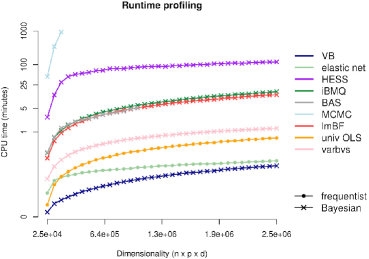
D.3 Runtime profiling
We report a runtime profiling of the different methods for a range of problem sizes (). Figure 11 displays the run times in minutes, averaged over replications. We do not aim to provide precise and exhaustive comparisons, since the methods all depend on parallelism and convergence characteristics that are not directly comparable. All methods were run serially, in an attempt to treat them on an equal footing. This choice could be challenged, as some approaches are more parallelizable than others, but the number of cores used for the latter represents an additional setting that would come into play with a potentially large impact on the measures. The number of chains for MCMC inferences also matters: HESS (Richardson et al., 2010) is run with three chains (following its authors’ choice made in their simulations); the other MCMC inferences are based on a single chain. Finally, the runtime may also greatly vary depending on the chosen chain length: the latter is adaptively selected by the Bayesian multiple regression method BAS (Clyde, 2016), and, based on preliminary convergence diagnostics, it is set to samples for HESS, iBMQ (Scott-Boyer et al., 2012) and the MCMC inference on our model using OpenBUGS (Spiegelhalter et al., 2007). In practice, the number of samples needed until convergence may increase greatly with the problem size, a fact that was not accounted for in this profiling. Hence, by adequately increasing the chain lengths when considering larger dimensionalities, we expect the curves of Figure 11 corresponding to the MCMC approaches to deviate more widely from that of our method. With these serial settings, our approach is faster than all Bayesian and frequentist methods. MCMC inference for our model is the slowest of all tested methods, which underlines the intractability of MCMC sampling for large problems. Inference for HESS is faster, but still more than times slower than our variational approach. Our method is also about times faster than applications (one for each outcome) of the varbvs method (Carbonetto and Stephens, 2012) but the runtime of the varbvs procedure can be reduced using multiple cores.
Appendix E Details on the real data problem
E.1 Clinical study and preprocessing of the mQTL data analysis
Diogenes (Larsen et al., 2010) is a large clinical dietary intervention study, which enrolled roughly overweight subjects from European centers. The subjects were assigned to a -week weight-loss program followed by months of supervised ad-libitum diet, meant as a weight-maintenance phase. For the -month period, individuals were randomized into five intervention groups, whose diets differed in their macronutrient and glycemic load content. The clinical trial had the broad objective of elucidating whether certain macronutrient compositions are more successful in weight maintenance than others. It gathered data on genetic variants, gene, protein and metabolite expression. In addition, more than clinical, anthropometric and behavioural variables were made available for each individual. When meaningful to do so, the data were collected at three time points, reflecting different stages of the dietary treatment.
In Section 5.3, we performed an mQTL analysis which involves tag SNPs from Illumina HumanCore chips (about 300k SNPs) and metabolites from plasma obtained by liquid chromatography-mass spectrometry (LC-MS). We excluded SNPs having missing values, minor allele frequency below , call rate below , or violating the Hardy–Weinberg equilibrium. Moreover, subjects having gender discrepancy (e.g., subject recorded as male but being homozygous for each X chromosome marker), abnormal autosomal heterozygosity or whose genomes were too close to each other (IBS) were also excluded. Additional subjects were removed after applying the Tukey method for outlier detection (Tukey, 1949), based on the metabolomic data. Metabolite expression levels were log2-transformed, and had no missing values. After these quality checks, the data consisted of SNPs and metabolite expression levels, for individuals.
E.2 Permutation-based Bayesian false discovery rate estimation
We provide details on the false discovery rate estimation procedure applied in Section 5.3 to compare our method with the varbvs method of Carbonetto and Stephens (2012) on the real data. We use the two-group mixture approach proposed by Efron (2008) in the context of microarray data analysis: we simultaneously consider null hypotheses and their corresponding test statistics, which we assume to follow a mixture distribution
where is the prior probability for a null case, and and are the null and non-null cumulative distribution functions. The “Bayesian false discovery rate” for some threshold is the posterior probability that a rejected null hypothesis (i.e., test statistic exceeding ) is a false positive,
| (25) |
where and . We derive estimates of (25) based on the posterior probabilities of inclusion quantifying the associations between each covariate-response pair. Specifically, we obtain an empirical null distribution by running our algorithm (with the same hyperparameters as those used for the actual inference) on datasets with permuted outcome sample labels and compute, for a grid of thresholds ,
| (26) |
where we conservatively set to in (25). As the posterior probabilities of inclusion obtained by applying varbvs times (one multiple regression for each outcome) are not identically calibrated across all estimations, we use adaptive thresholds on the columns of the varbvs posterior probabilities of inclusion matrix,
To find thresholds corresponding to preselected false discovery rates, we fit a cubic spline to the estimates (26) previously obtained for .
E.3 Biological evidence for the mQTL analysis findings
We support the findings obtained by our method for the mQTL data analysis with external association results from the following online databases:
-
•
GWAS catalog (Welter et al., 2014);
-
•
UCSC genome browser (Karolchik et al., 2003);
-
•
GTEx (Lonsdale et al., 2013); and
-
•
GeneCards (Rebhan et al., 1998).
We find direct or indirect links with metabolic activities for of the SNPs declared as “active’ by our method: SNPs , , , , , , , , , , and have been identified as associated with BMI, diverse diabetic or obesity diseases, fatty acid, sphingolipid or phospholipid levels, either from direct genome-wide association analyses or through protein coding genes for which they were reported as eQTLs.
E.4 Replication of the mQTL data analysis
In this appendix, we replicate the real data analysis of Section 5.3 on a simulated dataset (with twice as many outcomes and slightly more observations), which can be found on Figshare (https://dx.doi.org/10.6084/m9.figshare.4509755.v1). The analysis can be reproduced using the code available on GitHub (https://github.com/hruffieux/mQTL_analysis_example), provided that a machine with adequate RAM memory (about G for this large problem) is used.
To best mimic the real mQTL data used in Section 5.3, we simulate SNPs based on the sample minor allele frequencies of the real tag SNPs and we reproduce their dependence structure by blocks of consecutive SNPs according to the discussion of Appendix D.1. We also simulate normally distributed outcomes with equicorrelation by blocks using correlation coefficient ; this block structure is similar to that of the real metabolite data. To induce a realistic pleiotropic pattern, we simulate associations between SNPs and metabolites (randomly chosen) taking the block-wise dependence structure of the latter into account: the probability that a given active SNP is associated with a given active outcome varies across blocks, so correlated metabolites are either all highly likely or all less likely to be associated with the SNP. The average proportion of metabolic variance explained with each association is (but more associations explain less than this, as discussed in Appendix D.1). We generate observations.
| # TP: | |||
| Permutation-based FDR (%) | VB | varbvs | VB varbvs |
| 5 | 13 | 18 | 13 |
| 10 | 26 | 26 | 23 |
| 15 | 32 | 32 | 28 |
| 20 | 38 | 32 | 28 |
| 25 | 47 | 33 | 29 |


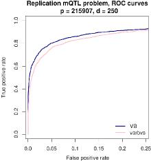
We apply the permutation analysis described in Section 5.3 to varbvs and our method and again obtain a more powerful selection for our method compared to varbvs at estimated FDR of and (Table 5 and Figure 13). Because simulated data are used, we can further support the overall superiority of our method with ROC curves, see Figure 12.