Anisotropic XY antiferromagnets in a field

Abstract

Classical anisotropic XY antiferromagnets in a field on square and simple cubic lattices are studied using mainly Monte Carlo simulations. While in two dimensions the ordered antiferromagnetic and spin–flop phases are observed to be separated by a narrow disordered phase, a line of direct transitions of first order between the two phases and a bicritical point are found in three dimensions. Results are compared to previous findings.

1 Introduction

Uniaxially anisotropic antiferromagnets in a magnetic field have been studied quite extensively in the past, both experimentally and theoretically. Typically, they display, at low temperatures, the antiferromagnetic (AF) phase and, when increasing the field, the spin–flop (SF) phase Neel ; Gorter . In addition, more complicated structures, like biconical KNF ones, have been observed. The various ordered phases may lead to interesting multicritical behavior, including bi– and tetracritical points KNF ; LF ; FN ; Aha2 .

Experimentally, several antiferromagnets with uniaxial anisotropy have been investigated, three–dimensional magnets SF ; RG ; FK ; OU ; FPB , such as MnF₂ and GdAlO₃, as well as quasi two–dimensional magnets SCD ; T ; BS ; BSL .

Much of the theoretical work is based on analyzing the prototypical classical Heisenberg model with uniaxial anisotropy, the XXZ model, in a field, plus, possibly, further anisotropy terms, such as single–ion anisotropies. Especially, mean–field approximation Gorter ; LF , Monte Carlo simulations LanBin ; Holt1 ; hws ; Zhou2 ; hs ; sel ; htl ; fp , and renormalization group calculations KNF ; FN ; CPV ; Folk ; Eich have been applied.

In this article, we shall deal with the anisotropic XY antiferromagnet in a field. The $x$–axis is taken to be the easy axis and the field acts on the $x$–component of the spins. The model is a variant of the much studied uniaxially anisotropic three–component XXZ antiferromagnet in a field, with the field along the easy axis, the $z$–direction. In a previous paper, the two–dimensional version, on the square lattice, of the XY model had been studied, applying ground state considerations and Monte Carlo techniques hs . At the field separating the AF and SF phases, the ground state has been found to be highly degenerate due to the presence of biconical (or, more precisely, non–collinear, biangular or bidirectional, BD) structures. At finite temperatures, $T>0$, these structures seem to lead to a disordered phase between the AF and SF phases, similar to the situation in the two–dimensional XXZ Heisenberg antiferromagnet. Here, we shall briefly reconsider this case. Our main emphasis will be on the anisotropic XY model on the simple cubic lattice. To our knowledge, no prior analysis exists. In particular, the existence and nature of the possible bicritical point, at which the AF, SF, and paramagnetic phases are expected to merge, in analogy to the XXZ antiferromagnet, will be studied.

The paper is organised as follows: In the next section, the anisotropic XY model will be introduced and ground state properties will be discussed. Then, results for the model on the square lattice will be presented, followed by our large–scale simulation findings for the three-dimensional case. A short summary concludes the article.

2 The model

The anisotropic XY antiferromagnet in a field is described by the Hamiltonian

$${\cal H}_{\mathrm{XY}}=J\sum\limits_{i,j}\left[\,S_{i}^{x}S_{j}^{x}+\Delta S_{i}^{y}S_{j}^{y}\,\right]\;-\;H\sum\limits_{i}S_{i}^{x}$$ (1)

where the first sum runs over all pairs of neighbouring sites, $i$ and $j$, of the lattice, with the second sum running over all lattice sites. $J>0$ is the antiferromagnetic coupling constant, $\Delta<1$ is the anisotropy parameter, and $H$ is the external field along the easy axis, the $x$-axis. $S_{i}^{\alpha}$, $\alpha$=$x$ and $y$, are the two components of the classical spin vector of length one.

Figure 1: Ground state configurations: (a) antiferromagnetic (AF), (b,d) spin–flop (SF), and (c) biconical as well as (e) bidirectional (BD) configurations. (a,d,e) occur in the anisotropic XY, (a,b,c) in the uniaxially anisotropic XXZ antiferromagnet. The tilt angles are defined with respect to the easy axis, being the $x$–axis in the XY and the $z$–axis in the XXZ case.

We shall consider mainly the model on a simple cubic lattice ($d=3$), but some results for the square lattice ($d=2$) will also be discussed comparing them to previous findings hs . In both cases, the ground states, at zero temperature, $T=0$, see Figure 1, may be determined in a straightforward way LF ; hs ; TM . For small fields, $H<H_{c1}$, the AF structure is stable, in which neighbouring sites belong to different sublattices, $A$ and $B$, where the $x$–components of $A$– and $B$–spins point in opposite directions. The $y$–component vanishes at all sites. At intermediate fields, $H_{c1}<H<H_{c2}$, one encounters the SF structure, where the $x$–components of the spins on both sublattices are equal, being smaller than one, while the antiferromagnetic sublattice structure shows up in the $y$–components. At large fields, $H>H_{c2}$, all spins are aligned parallel to the field, with vanishing $y$–component of the spin vectors. At $H=H_{c1}$, the AF, the SF, and BD configurations form ground states. In the highly degenerate BD configurations, the spins on the two sublattices, $A$ and $B$, are tilted with respect to the field direction, the $x$–axis. The resulting two tilt angles, say, $\Theta_{A}$ and $\Theta_{B}$, are interrelated interpolating continuously between the AF and SF structures. The exact relation depends on the anisotropy parameter $\Delta$. Of course, in the SF limit, one has $\Theta_{A}=\Theta_{B}=\Theta_{SF}(H)>0$.

At non-zero temperatures, one expects, among others, phase transitions in the Ising universality class from the disordered phase to the AF and SF phases. The longitudinal staggered magnetization, describing the antiferromagnetic ordering of the $x$–component of the spins on the $A$– and $B$–sublattices, is the order parameter in the AF phase. The transversal staggered magnetization describes the antiferromagnetic ordering of the $y$–component of the spins in the SF phase, in which the $x$–component has the same value on both sublattices. Accordingly, a possible bicritical point is expected to belong to the $n=2$ or XY universality class KNF ; FN . This behaviour is in marked contrast to the situation in the anisotropic XXZ antiferromagnet in a field, along the $z$–axis. There the SF phase is described by an antiferromagnetic ordering of the two components perpendicular to the $z$–component of the spins, implying a transition to the paramagnetic phase in the XY universality class. Of course, the transition from the paramagnetic to the AF phase belongs to the Ising universality class, in the XXZ case as well. Thence, a possible bicritical point would fall into the $n=3$ or Heisenberg universality class KNF ; FN .

To study the phase diagram, in the $(k_{B}T/J,H/J)$ plane, of the 2d and 3d XY antiferromagnets, we did extensive Monte Carlo (MC) simulations, using the standard Metropolis algorithm LB . Lattices with $L^{d}$ sites were considered, with $L$ ranging from 10 to 200 for $d=2$, and from 8 to 40 for $d=3$. In all cases, full periodic boundary conditions were employed. As usual, finite–size extrapolations were done to obtain estimates for the thermodynamic limit. Typically, runs of, at least, $10^{7}$ MC steps per site (MCS) were performed, averaging over a few realizations, by using different random numbers, to estimate error bars. Here, error bars are usually smaller than the size of the symbols shown in the figures. Of course, close to the phase transition, larger lattices may require longer runs to take into account critical fluctuations and critical slowing down LB .

We recorded, among others, quantities related to the longitudinal staggered magnetisation $M_{st}^{x}$ defined by $M_{st}^{x}=(S_{A}^{x}-S_{B}^{x})/2$, and the corresponding transversal staggered magnetization for the $y$ component of the spins. In particular, thermal averages over the second moments of the magnetizations are expected to signal the transitions to the AF and SF phases. Actually, these transitions may be detected quite easily and reliably by the Binder cumulant Binder

$$U^{x,y}=1-<(M_{st}^{x,y})^{4}>/(3<(M_{st}^{x,y})^{2}>)$$ (2)

where the brackets denote thermal averages. The transition from the disordered phase to the AF phase can be determined by $U^{x}$, and that to the SF phase can be determined by $U^{y}$. To detect a possible bicritical point in the $n=2$ or XY universality class, we also computed the analoguous Binder cumulant $U^{xy}$, invoking the second and fourth moments of the total staggered magnetization $M_{st}=\sqrt{((M_{st}^{x})^{2}+(M_{st}^{y})^{2})}$.

We also recorded the longitudinal and transversal staggered susceptibilties, obtained, as usual, from the fluctuations of the corresponding magnetizations. Further interesting information on the thermal behavior of the model follows from the specific heat, $C$, determined from the energy fluctuations, as well as histograms. In particular, we computed probability functions of the tilt angles, such as the probability $p(\Theta)$ for encountering the tilt angle $\Theta$ at an arbitrary site and the probability $p_{2}(\Theta_{A},\Theta_{B})$ for finding the two angles, $\Theta_{A}$ and $\Theta_{B}$, at neighbouring sites of the lattice, as before hs .

3 Phase diagrams

We shall first briefly discuss previous and new MC findings for the 2d case, presenting evidence for a narrow disordered phase separating the AF and SF phases. The main emphasis will be on the 3d model, for which a qualitatively different topology of the phase diagram is observed. In fact, our simulation data suggest the existence of a bicritical point, at which the AF, SF, and paramagnetic phases meet. In both cases, we set the anisotropy parameter $\Delta=0.8$.

3.1 Anisotropic XY antiferromagnet on a square lattice

The phase diagram of the anisotropic XY antiferromagnet in a field on a square lattice has been determined before hs , comprising the AF, SF, and paramagnetic phases. It is depicted in Figure 2, setting the anisotropy parameter $\Delta$ equal to 0.8. The characteristic fields for the ground states are $H_{c1}/J=2.4$ and $H_{c2}/J=7.2$. The transition lines of the AF and SF phases to the disordered phase, having confirmed to be in the Ising universality class, approach each other rather closely at $k_{B}T/J\approx 0.68$ and $H/J\approx 2.47$.

Figure 2: Phase diagram of the anisotropic XY antiferromagnet on the square lattice with $\Delta=0.8$. From Reference 20.

In principle, the two lines might meet at a bicritical point in the XY or Kosterlitz–Thouless KT universality class, with a line of transitions of first order between the AF and SF phases at lower temperatures. Note that such a topology is excluded for the two–dimensional XXZ antiferromagnet, where the bicritical point would belong to the Heisenberg universality class. In fact, the existence of such a point at $T>0$ is excluded by the well–known theorem of Mermin and Wagner MW .

In our present study, we searched for possible evidence, whether there is a bicritical point in the anisotropic XY model on a square lattice. In particular, we did MC simulations at the temperatures $k_{B}T/J$ = 0.7, 0.6, and 0.4.

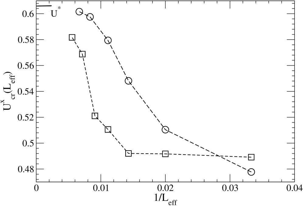
Figure 3: Finite–size dependence of the crossing points of the longitudinal Binder cumulants $U_{cr}^{x}(L_{eff})$ at $k_{B}T/J=0.6$ (squares) and $0.7$ (circles). The value of the critical cumulant for the Ising case $U^{*}=0.61069...$ is indicated.

The Binder cumulants $U^{x,y}$ turned out to be very useful in investigating the low–temperature region. We monitored the crossing points $U_{cr}(L_{eff})$ of the cumulants for two successive square lattices with linear dimensions $L_{1}$ and $L_{2}$, assigning an effective length $L_{eff}=(L_{1}+L_{2})/2$. In general Binder , one expects $U_{cr}$ to occur in the thermodynamic limit at the phase transition, with the critical value $U^{*}$. In the case of phase transitions in the 2d Ising universality class, employing full periodic boundary conditions and considering systems with spatially isotropic spin–spin correlations cd ; sesh , one has $U^{*}$= 0.61069 ..sesh ; kabl .

In Figure 3, results for the crossing points of the longitudinal Binder cumulant $U^{x}$ at $k_{B}T/J$ = 0.6 and 0.7, with lattice sizes ranging from $L$= 20 to 200, are depicted. The typical critical value, $U^{*}$= 0.61069.., seems to be approached for both temperatures, with smaller finite–size effects at the higher temperature. Similar observations hold for the transversal cumulant. Accordingly, the two transitions are seen to be Ising–like. Note that at $k_{B}T/J$= 0.6, the two distinct transitions occur at about $H/J$ = 2.4505 and 2.4525, as estimated from the size–dependence of the crossing points, $U_{cr}^{x}$ and $U_{cr}^{y}$. The disordered phase between the AF and SF phases becomes more and more narrow, as the temperature is lowered, see also Figure 2.

The existence of that narrow disordered phase had been previously hs inferred from histograms of the probability $p_{2}$. $p_{2}$ describes the relation between the tilt angles at neighbouring sites, as stated above. Actually, at the temperature $k_{B}T/J=0.4$, in an extremely small range of fields, the dominant configurations have neither an AF nor SF character, but they are of BD type. The disordered phase had been argued to be due to BD fluctuations caused by the highly degenerate ground state at $H_{c1}$.

Indeed, the present simulations provide additional evidence against a transition of first order between the AF and SF phases at such low temperatures. For example, the longitudinal and transversal Binder cumulants are expected to become strongly negative near a first–order transition BiLa , even diverging to minus infinity in the thermodynamic limit. We do not observe such a behavior.

Moreover, we studied the maximal specific heat $C_{max}$, close to the AF–SF transition as a function of the lattice size, $L$. At a first order transition in two dimensions, $C_{max}$ is predicted FiBe to grow, for sufficiently large lattices, like $C_{max}\propto L^{2}$. On the other hand, at an Ising–like transition in two dimensions, there is only a logarithmic increase. Actually, we fitted the simulation data for $C_{max}(L)$ to a power law, $C_{max}\propto L^{X}$. We determined the effective exponent $X_{eff}(L)=d\ln C_{max}/d\ln L$. Simulations, at $k_{B}T/J$ = 0.4 and 0.6, are performed at discrete values of $L$, ranging from 20 to 200. Data for successive sizes, $L_{1}$ and $L_{2}$, are fitted to the discretized effective exponent $X_{eff}(L_{e})$, with $L_{e}=\sqrt{(L_{1}\times L_{2})}$. We find rather small effective exponents, being, at most, about 0.25, far from the quadratic behavior characterising a transition of first–order.

In conclusion, for the anisotropic XY antiferromagnet on a square lattice, we find no evidence for a direct transition of first order between the AF and SF phases down to $k_{B}/J=0.4$. Accordingly, there is no indication for a bicritical point.

3.2 Anisotropic XY antiferromagnet on a simple cubic lattice

The crucial part of the phase diagram for the 3d anisotropic XY model in a field is shown in Figure 4. It summarizes present MC findings, setting the anisotropy parameter $\Delta$ equal to 0.8. At zero temperature, the AF configuration is stable up to $H_{c1}/J=3.6$ and the SF structure is stable up to $H_{c2}/J=10.8$.

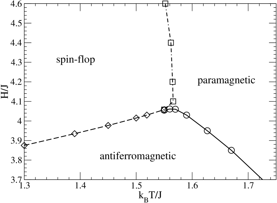
Figure 4: Phase diagram of the XY antiferromagnet with $\Delta=0.8$ on the simple cubic lattice.

The transition lines between the disordered paramagnetic phase and the two orderded phases AF and SF phases are believed to belong to the Ising universality class. In fact, our estimates for the critical exponents of the staggered magnetizations and susceptibilities as well as of the specific heat agree with the Ising values Vic . Furthermore, for both transitions, the critical Binder cumulants, $U^{*}$, are found to be close to the characteristic value for isotropic phase transitions of 3d Ising type, $U^{*}\approx 0.465$ Hb .

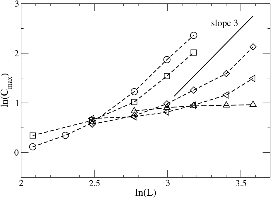
Figure 5: Maximal specific heat, $C_{max}$, versus lattice size, $L$, near the AF–SF transition at $k_{B}T/J$ = 1.0 (circles), 1.3 (squares), 1.45 (diamonds), 1.50 (triangles left), and 1.55 (triangles up). The straight line corresponds to $C_{max}\propto L^{3}$.

The most interesting aspect of the phase diagram concerns the existence, location, and characteristics of the bicritical point, at which the AF, SF, and paramagnetic phases may meet.

To identify a, possibly, first–order transition between the AF and SF phases at low temperatures, we monitored the size–dependence of the maximum in the specific heat, $C_{max}$. A first transition of first order is expected FiBe to be signalled by a divergence of the form $C_{max}\propto L^{3}$, for sufficiently large lattice sizes. In contrast, at a continuous transition in three dimensions, one expects a power–law behavior with an exponent $\alpha/\nu$, with $\alpha$ and $\nu$ being the standard critical exponents. For an Ising–type transition in 3d Vic , one obtains $\alpha/\nu\approx 0.175$. As depicted in Figure 5, the size–dependence typical for a first–order transition is observed to be approximated closely at low temperatures. For instance, at $k_{B}T/J$ = 1.0, the cubic size dependence, characteristic for a first–order transition, is approached already for $L$ = 16. Increasing the temperature, the crossover towards the (almost) cubic behaviour is shifted to larger lattices, being about $L$ = 30 at $k_{B}T/J$ = 1.45. Obviously, at higher temperatures, as shown in Figure 5 for $k_{B}T/J=1.5$, it becomes more and more demanding to reach the asymptotic regime. Presumably, the difficulty is related to the increase in the correlation length at the first–order transition when getting closer to the bicritical point. Actually, at the bicritical point in the XY universality class, one expects no divergence in $C$, but a cusp–like singularity, with the corresponding standard critical exponent $\alpha$ being slightly negative Vic . Indeed, see Figure 5, at $k_{B}T/J=1.55$, $C_{max}$ increases only slightly with the lattice size, indicating, probably, the closeness of the bicritical point.

Another signature of the first–order transition at low temperatures is provided by the longitudinal and transversal Binder cumulants, $U^{x}$ and $U^{y}$. In fact, both quantities display, close to the boundary between the AF and SF phases, negative minima, choosing temperatures $k_{B}T/J$ ranging from 1.0 to 1.50. Lattices with $L$ up to 36 were considered. The minima became more pronounced, when lowering the temperature, reflecting the fact that then the transition gets more strongly of first order, with a smaller correlation length, in agreement with the behavior of the specific heat, as discussed above. By increasing the lattice size, the minima are getting deeper. In fact, in the thermodynamic limit, the cumulant is predicted to be minus infinity at the phase transition of first order BiLa .

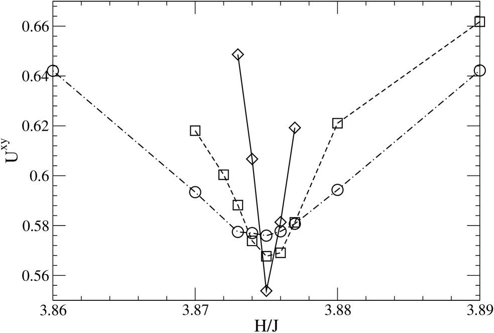
Figure 6: Binder cumulant $U^{xy}$ at constant temperature, $k_{B}T/J$ = 1.3, as a function of the field $H/J$ near the AF–SF transition for lattices with $L$ =16 (circles), 20 (squares) and 30 (diamonds).

The data on the specific heat $C$ suggest that the transition between the AF and SF phases is of first order up to temperatures of, at least, about $k_{B}T/J\approx 1.5$. To locate the bicrital point and to characterize its nature, the Binder cumulant $U^{xy}$ turns out to be quite useful as well. Its critical value, at a transition point in the XY–universality class in three dimensions, has been estimated HT to be $U^{(xy)*}\approx 0.586$.

Of course, $U^{xy}$ is expected to approach, for large lattices, in both ordered phases the limiting value 2/3. When the transition between the AF and SF phases is of first order, as suggested by the specific heat, the cumulant displays, fixing the temperature and varying the field (or vice versa), a minimum close to the transition, $U^{xy}_{min}$, as exemplified in Figure 6. When increasing the lattice size, the minimum is, eventually, lowered, falling clearly below the value, 0.586, characterising the XY universality class. Results of the present simulations on the size–dependence of the height of the minimum for various temperatures and fields are depicted in Figure 7.

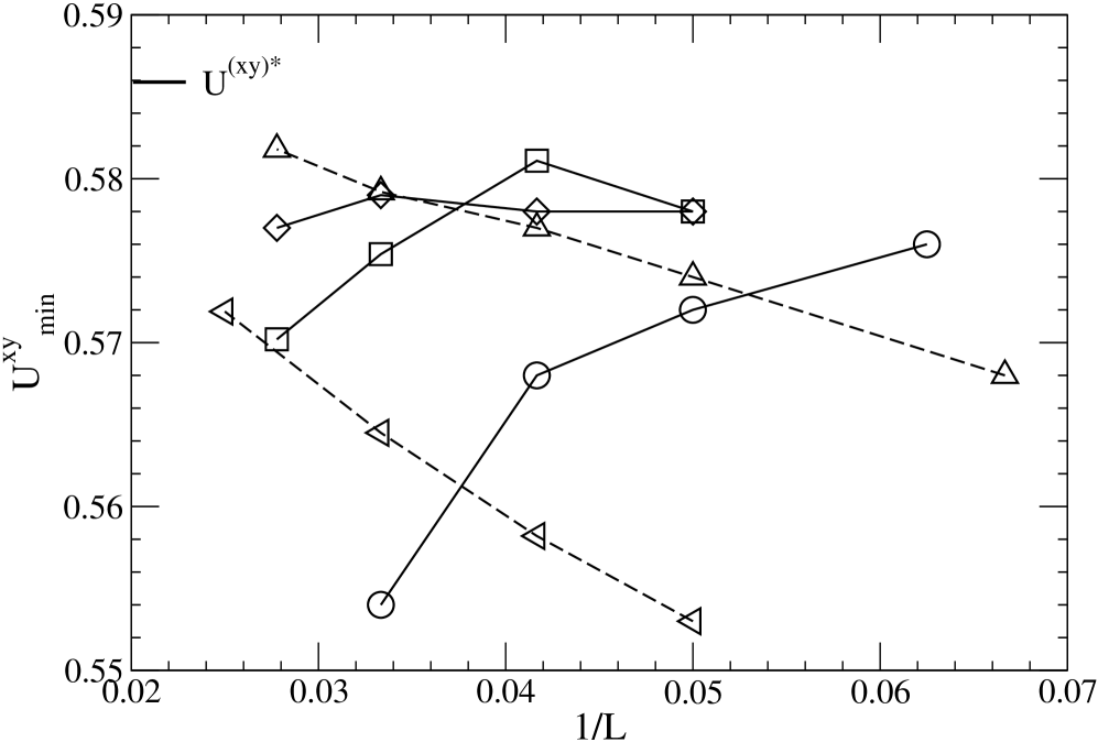
Figure 7: Minimum of the xy–cumulant $U^{xy}_{min}$ as a function of lattice size $L$ for various temperatures $k_{B}T/J$ = 1.3 (circles), 1.45 (squares), 1.5 (diamonds), and 1.55 (triangles left) as well as for fixed field $H/J$ = 4.03 (triangles up). The critical cumulant in the XY universality class occurs at $U^{(xy)*}\approx 0.586$ HT .

Perhaps most interestingly, Figure 7 shows a rather drastic change in the size dependence of the height of the minimum, when getting closer to the bicritical point. Eventually, $U^{xy}_{min}$ starts to increase for large lattices. It seems to approach, for sufficiently large lattices, the characteristic value of the 3d XY universality class, $U^{(xy)*}\approx 0.586$, in the temperature range between about $k_{B}T/J$ = 1.51 and 1.55. The lower bound is inferred from the simulation data when fixing the field at $H/J$ = 4.03, with the corresponding phase transition occurring at $k_{B}T/J\approx 1.518$. Accordingly, the present simulations are consistent with the existence of a bicritical point of XY type in the three–dimensional model. The result confirms the previous theoretical prediction KNF ; FN on the nature of the bicritical point, based on renormalization group calculations. Note that at even higher temperatures, either the two transition lines of the AF and SF phases to the paramagnetic phase are well separated or there is only the transition to the AF phase, as depicted in Figure 3. Then, the transition is no longer signalled by a minimum in $U^{xy}$.

Of course, to explore, in detail, finite–size effects in the crossover region in the vicinity of the bicritical point, data of very high accuracy for larger lattices would be desirable. This feature, however, is beyond the scope of our study.

4 Summary

We conclude that the topology of the phase diagram, in the ($k_{B}T/J,H/J$) plane, of the anisotropic XY antiferromagnet depends significantly on the lattice dimension. For the square lattice, in agreement with a previous study, we find no evidence for a bicritical point. Instead, in between the AF and SF phases, there is a narrow intervening paramagnetic phase down to the lowest temperatures we considered. In contrast, for the simple cubic lattice, we find a line of direct transitions of first order between the two ordered phases, leading, eventually, to a bicritical point.

We locate the bicritical point at $k_{B}T/J\approx 1.53\pm 0.02$, based on finite–size analyzes for the specific heat and Binder cumulants. The point belongs to the XY universality class.

The qualitatively different phase diagrams in two and three dimensions may be explained by the bidirectional configurations, leading to the highly degenerate ground state at the field separating the AF and SF structures. In two dimensions, these configurations seem to surpress the direct transition between the AF and SF phases, while they are thermally less relevant in three dimensions. Such a feature has been seen to hold in the related XXZ Heisenberg antiferromagnet in a field as well. In that case, the existence of a bicritical point (belonging to the Heisenberg universality class) in two dimensions is already excluded by the Mermin–Wagner theorem.

We should like to thank especially Kurt Binder, David Landau, Reinhard Folk, and Martin Holtschneider for useful information, remarks, and discussions on the topic of this article. The article is dedicated to Wolfhard Janke on the occasion of his sixtieth birthday. We thank him for very helpful and pleasant interactions.

References

- (1) L. Néel, Ann. Phys.(Paris) 18, 5 (1932).
- (2) C. J. Gorter and T. van Peski-Tinbergen, Physica (Utr.) 22, 273 (1956).
- (3) J. M. Kosterlitz, D. R. Nelson, and M. E. Fisher, Phys. Rev. B 13, 412 (1976).
- (4) K.-S. Liu and M. E. Fisher, J. Low. Temp. Phys. 10, 655 (1973).
- (5) M. E. Fisher and D. R. Nelson, Phys. Rev. Lett. 32, 1350 (1974).
- (6) A. Aharony, J. Stat. Phys. 110, 659 (2003).
- (7) Y. Shapira and S. Foner, Phys. Rev. B 1, 3083 (1970).
- (8) H. Rohrer and Ch. Gerber, Phys. Rev. Lett. 38, 909 (1977).
- (9) G. P. Felcher and R. Kleb, Europhys. Lett. 36, 455 (1996).
- (10) K. Ohgushi and Y. Ueda, Phys. Rev. Lett. 95, 217202 (2005).
- (11) R. S. Freitas, A. Paduan–Filho, and C. C. Becerra, J. Phys.: Condens. Matter 28, 126007 (2016).
- (12) K. Y. Szeto, S. T. Chen, and G. Dresselhaus, Phys. Rev. B 33, 3453 (1986).
- (13) T. Thio, C. Y. Chen, B. S. Freer, D. R. Gabbe, H. P. Jenssen, M. A. Kastner, P. J. Picone, N. W. Preyer, and R. J. Birgeneau, Phys. Rev. B 41, 231 (1990).
- (14) R. Leidl, R. Klingeler, B. Büchner, M. Holtschneider, and W. Selke, Phys. Rev. B 73, 224415 (2006); T. Kroll, R. Klingeler, J. Geck, B. Büchner, W. Selke, M. Hücker, and A. Gukasov, J. Magn. Magn. Mat. 290, 306 (2005).
- (15) N. Barbero, T. Shiroka, C. P. Landee, M. Pikulski, H.–R. Ott, and J. Mesot, Phys. Rev. B 93, 054425 (2016).
- (16) K. Binder and D. P. Landau, Phys. Rev. B 13, 1140 (1976); D. P. Landau and K. Binder, Phys. Rev. B 17, 2328 (1978).
- (17) M. Holtschneider, W. Selke, and R. Leidl, Phys. Rev. B 72, 064443 (2005).
- (18) M. Holtschneider, S. Wessel, and W. Selke, Phys. Rev. B 75, 224417 (2007).
- (19) C. Zhou, D. P. Landau, and T. C. Schulthess, Phys. Rev. B 76, 024433 (2007).
- (20) M. Holtschneider and W. Selke, Eur. Phys. J. B 62, 147 (2008).
- (21) W. Selke, Phys. Rev. E 83, 042102 (2011); Phys. Rev. E 87, 014101 (2013).
- (22) S. Hu, S.–H. Tsai, and D. P. Landau, Phys. Rev. E 89, 032118 (2014).
- (23) R. T. S. Freire and J. A. Plascak, Phys. Rev. E 91, 032146 (2015).
- (24) P. Calabrese, A. Pelissetto, and E. Vicari, Phys. Rev. B 67, 054505 (2003).
- (25) R. Folk, Yu. Holovatch, and G. Moser, Phys. Rev. E 78, 041125 (2008).
- (26) A. Eichhorn, D. Mesterhazy, and M. M. Scherer, Phys. Rev. E 88, 042141 (2013).
- (27) H. Matsuda and T. Tsuneto, Prog. Theoret. Phys. Suppl. 46, 411 (1970).
- (28) D. P. Landau and K. Binder, A Guide to Monte Carlo Simulations in Statistical Physics (University Press, Cambridge, 2014).
- (29) K. Binder, Z. Phys. B 43, 119 (1981).
- (30) J. M. Kosterlitz and D. J. Thouless, J. Phys. C 6, 1181 (1973).
- (31) N. D. Mermin and H. Wagner, Phys. Rev. Lett. 17, 1133 (1966).
- (32) X. S. Chen and V. Dohm, Phys. Rev. E 70, 056136 (2004).
- (33) W. Selke and L. N. Shchur, J. Phys. A: Math. Gen. 38, L739 (2005).
- (34) G. Kamieniarz and H. W. J. Blöte, J. Phys. A: Math. Gen. 26, 201 (1993).
- (35) K. Binder and D. P. Landau, Phys. Rev. B 30, 1477 (1984); A. W. Sandvik, Phys. Rev. Lett. 104, 177201 (2010).
- (36) M. E. Fisher and A. N. Berker, Phys. Rev. B 26, 2507 (1982); W. Janke, in: B. Dünweg, D. P. Landau, and A. I. Milchev (eds.), Computer Simulations of Surfaces and Interfaces, Kluwer Academics (2003), p.111-135.
- (37) M. Hasenbusch, Phys. Rev. B 82, 174434 (2010).
- (38) A. Pelissetto and E. Vicari, Phys. Reports 368, 549 (2002).
- (39) M. Hasenbusch and T. Török, J. Phys. A: Math. Gen. 32, 6361 (1999); M. Campostrini, M. Hasenbusch, A. Pelissetto, P. Rossi and E. Vicari, Phys. Rev. B 63, 214503 (2001).