Intramode correlations enhanced phase sensitivities in an SU(1,1) interferometer

Abstract

We theoretically derive the lower and upper bounds of quantum Fisher information (QFI) of an SU(1,1) interferometer whatever the input state chosen. According to the QFI, the crucial resource for quantum enhancement is shown to be large intramode correlations indicated by the Mandel $Q$-parameter. For a photon-subtracted squeezed vacuum state with high super-Poissonian statistics in one input port and a coherent state in the other input port, the quantum Cramér-Rao bound of the SU(1,1) interferometer can beat $1/\langle\hat{N}\rangle$ scaling in presence of large fluctuations in the number of photons, with a given fixed input mean number of photons. The definition of the Heisenberg limit (HL) should take into account the amount of fluctuations. The HL considering the number fluctuation effect may be the ultimate phase limit.

I Introduction

Quantum mechanics provides a fundamental limit on the achievable measurement precision, optimized over all possible estimators, measurements and probe states. The paradigmatic example is the optical phase estimation. When the number of particles in the input state is fixed and equal to $N$, the phase sensitivity is limited by two bounds. One is the standard quantum limit (SQL), $1/\sqrt{N}$, which is due to the classical nature of the coherent state and can be beaten by quantum-mechanical effects. Another is the fundamental Heisenberg limit (HL) which is given by $1/N$ and cannot be beaten. Analogously, for a fixed mean photon number $\langle\hat{N}\rangle$, measurement accuracy also has a fundamental HL. However, the violation of $1/\langle\hat{N}\rangle$ scaling of the optimal accuracy is possible in presence of large fluctuations in the number of probes Sharpio ; Pasquale . Then definition of the HL should take into account the amount of photon number fluctuations hofmann ; hyllus ; pezze2015 .

Using quantum measurement techniques to beat the SQL, has been received a lot of attention in recent years Helstrom67 ; Holevo82 ; Caves81 ; Braunstein94 ; Braunstein96 ; Lee02 ; Giovannetti06 ; Zwierz10 ; Giovannetti04 ; Giovannetti11 . The Mach-Zehnder interferometer (MZI) and its variants, which can be understood as a two-mode (two-path) interferometer, have been used as a generic model to realize precise measurement of phase Abbott . In order to avoid the vacuum fluctuations, Caves suggested to use the coherent and squeezed-vacuum light as input of a Mach-Zehnder interferometer to reach a sub-shot-noise sensitivity in 1981 Caves81 . Later, many quantum parameter estimation protocols have been proposed Giovannetti04 ; Giovannetti11 ; Toth . The enhancements obtained from employing quantum state can be divided into two parts according to the correlations Sahota : (1) intramode correlations which are provided by a large uncertainty in the photon number in each arm, such as the squeezed vacuum exhibits high intramode correlations due to nonclassical photon statistics; (2) intermode correlations, i.e., correlations between two paths which can be realized by mode entanglement. The NOON state, i.e., states of the form $(|N\rangle_{a}|0\rangle_{b}+e^{i\phi_{N}}|0\rangle_{a}|N\rangle_{b})/\sqrt{2}$ have been suggested to reach the HL scaling, in the phase-shift measurements $\Delta\phi_{\text{HL}}=1/N$ NOON ; Dowling . The enhancement of phase sensitivity with NOON state benefits from both intermode correlation and intramode correlation Knott . However, the intermode correlations can contribute at most a factor of $1/\sqrt{2}$ improvement in the phase precision, which was pointed out by Sahota and Quesada Sahota . But the intramode correlations have no upper bound Berrada , which naturally leads us to search and study quantum states with high intramode correlations.

In additional to the nonclassical input states with high intramode correlations, the nonlinear elements were also introduced in the linear interferometers to improve the measurement precision. Such a class of interferometers introduced by Yurke et al. Yurke86 is described by the group SU(1,1)-as opposed to SU(2), where the 50-50 beam splitters (BSs) in a traditional MZI was replaced by the nonlinear beam splitters (NBSs), such as optical parametric amplifiers (OPAs) or four-wave mixings (FWMs) (see Fig. 1). Recently, an improved theoretical scheme was presented by Plick et al. Plick who proposed to inject a strong coherent beam to “boost” the photon number. With a coherent state in one input port and a squeezed-vacuum state in the other input port using the method of homodyne detection, the phase sensitivity can approach $1/\langle\hat{N}\rangle$ scaling Li14 . Experimental realization of this SU(1,1) optical interferometer was reported by our group Jing11 . The noise performance of this interferometer was analyzed Ou ; Marino and under the same phase-sensing intensity condition the improvement of $4.1$ dB in signal-to-noise ratio was observed Hudelist . By contrast, an SU(1,1) atomic interferometer has also been experimentally realized with Bose-Einstein Condensates Gross ; Linnemann ; Peise ; Gabbrielli . An atom-photon interface can form an atom-light hybrid interferometer Yama ; Haine ; Szigeti ; Haine16 ; ChenPRL15 , where the atomic Raman amplification processes take the place of the beam splitting elements in a traditional MZI, and the losses performance of it was analyzed recently Yuan16 . Different from all-optical or all-atomic interferometers, the main feature is that both the optical field and atomic phases can be probed with optical interferometric techniques. In addition, the circuit quantum electrodynamics system was also introduced to form the SU(1,1) interferometer Barzanjeh , which provides a different method for basic measurement using the hybrid interferometers.

Recently, Lang and Caves Lang have proved that if one input port injected by a coherent state in an MZI, in the other input port the best injection state is a squeezed vacuum state with a given fixed mean number of photons. However, since the subtraction of photons from squeezed vacuum state has the effect of increasing the average photon number of the new field state, as well as the intramode correlations Biswas , Birrittella and Gerry Gerry suggested to use coherent and photon-subtracted squeezed vacuum states as input for quantum optical interferometry, and they found that it was still possible to attain higher sensitivity via photon subtraction from the squeezed state. The fact that photon subtraction via the annihilation operator leads to the average photon number counter-intuitively increasing was studied over twenty-years ago Ueda ; Mizrahi . Ueda et al. Ueda studied the average and variance of the field acted by the annihilation operator. The difference of average photon number between the remaining field $\bar{N}_{\text{sub}}$ and the initial field $\bar{N}$ is equivalent to the Mandel’s $Q$-parameter Mandel , i.e., $\bar{N}_{\text{sub}}-\bar{N}=Q$. For $Q>0$ ($-1<Q<0$), the photon statistics is super-Poissonian (sub-Poissonian), then the average photon number of the remaining field is shown to increase (decrease). For the Poissonian state (e.g., coherent light), the average photon number does not change ($\bar{N}_{\text{sub}}=\bar{N}$). Especially, due to generation of Schrödinger cat states the photon-subtracted squeezed vacuum states have been intensely studied theoretically Biswas ; Dakna ; Takeola and experimentally Ourjoumtsev ; Wakui ; Namekata ; Gerrits . Up to now three-photon subtraction from a squeezed vacuum state was reported Gerrits .

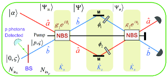
Figure 1: (Color online) The schematic diagram of the SU(1,1) interferometer. Two Nonlinear beam splitters (NBSs) take the place of two beam splitters in the traditional Mach-Zehnder interferometer, and $\hat{K}_{i}$ $(i=x,y,z)$ instead of $\hat{J}_{i}$ $(i=x,y,z)$ describe this interferometer in Schwinger representation. The input state $|\Psi_{\text{in}}\rangle$ injecting into the first NBS leads to output state $|\Psi\rangle$, then it is modified as $|\Psi_{\phi}\rangle$ by phase shift. $g_{1}$ ($g_{2}$) and $\theta_{1}$ ($\theta_{2}$) describe the strength and phase shift in the NBS process $1$ ($2$), respectively. $\hat{a}$ and $\hat{b}$ denote two light modes in the interferometer. A coherent state $|\alpha\rangle$ is in one input port and a squeezed-vacuum state $|0,\varsigma\rangle$ in the other input port of the SU(1,1) interferometer with total mean photon number of input $N_{\text{in}_{0}}$. A beam splitter with low reflectance and a single-photon resolution photo-detector are used to subtract $p$-photons from input squeezed vacuum state. The reflected photons that are detected herald a $p$-photon subtracted squeezed-vacuum state generation $|p,\varsigma\rangle_{b}$ $(\sim\hat{b}^{p}|0,\varsigma\rangle_{b})$. For a coherent light combined with a $p$-photon subtracted squeezed vacuum light as input, the total mean photon number of input is $N_{\text{in}_{p}}$. $\phi_{1}$, $\phi_{2}$: phase shift; M: mirrors; BS: beam splitter.

In this paper, we theoretically derive the lower and upper bounds of quantum Fisher information (QFI) Braunstein94 ; PezzBook of an SU(1,1) interferometer, in which the dominant resource for quantum enhancement is the large intramode correlations indicated by the Mandel $Q$-parameter. Furthermore, we study the phase sensitivities of the SU(1,1) interferometer for a coherent light combined with a photon-subtracted squeezed vacuum light and compare them with the HL.

Our article is organized as follows. In Sec. II, we give the QFI of the the SU(1,1) interferometer for general pure states input, and show that the metrological advantage of nonclassical light is primary the intramode correlations (high Mandel’s $Q$-parameter). Then we derive the QFI and give the quantum Cramér-Rao bound (QCRB) Helstrom67 ; Holevo82 of SU(1,1) interferometer with a coherent state $\otimes$ photon-subtracted squeezed vacuum state input. The comparison between the QCRB and the HL is given in Sec. III. In Sec. IV, we compare our proposal with that of Lang and Caves Lang . Finally, we conclude with a summary of our results.

II Quantum Fisher information

In general, it is difficult to optimize over the detection methods to obtain the optimal estimation protocols. One of the common ways to obtain the lower bounds in quantum metrology, is to use the method of the QFI. The so-called QFI is defined by maximizing the Fisher information over all possible measurement strategies allowed by quantum mechanics. It characterizes the maximum amount of information that can be extracted from quantum experiments about an unknown parameter using the best (and ideal) measurement device. It establishes the best precision that can be attained with a given quantum probe.

II.1 General description

An SU(1,1) interferometer is shown in Fig. 1, where NBSs replace the 50-50 BSs in a traditional MZI. We firstly give a brief review of the SU(1,1) interferometer introduced by Yurke et al. Yurke86 . The traditional MZI is called an SU(2) interferometer and can be understood as a two-mode (two-path) interferometer. The transformation by this interferometer is a rotation on angular momenta observables $\hat{J}_{x}=\hbar(\hat{a}^{\dagger}\hat{b}+\hat{a}\hat{b}^{\dagger})/2$, $\hat{J}_{y}=-i\hbar(\hat{a}^{\dagger}\hat{b}-\hat{a}\hat{b}^{\dagger})/2$, and $\hat{J}_{z}=\hbar(\hat{a}^{\dagger}\hat{a}-\hat{b}^{\dagger}\hat{b})/2$, where $\hat{a}$ $(\hat{a}^{{\dagger}})$ and $\hat{b}$ $(\hat{b}^{{\dagger}})$ are the annihilation (creation) operators corresponding to the two modes $a$ and $b$, respectively. For the SU(1,1) interferometer, the induced transformation on the input observables is that of the group SU(1,1). The Hermitian operators $\hat{K}_{x}=\hbar(\hat{a}^{\dagger}\hat{b}^{\dagger}+\hat{a}\hat{b})/2$, $\hat{K}_{y}=-i\hbar(\hat{a}^{\dagger}\hat{b}^{\dagger}-\hat{a}\hat{b})/2$, and $\hat{K}_{z}=\hbar(\hat{a}^{\dagger}\hat{a}+\hat{b}^{\dagger}\hat{b}+1)/2$ are introduced to describe the SU(1,1) interferometer. The initial state $|\Psi_{\text{in}}\rangle$ injecting into a NBS results in the output $|\Psi\rangle=e^{-i\xi\hat{K}_{x}}|\Psi_{\text{in}}\rangle$ where $\xi$ is the two-mode squeezed parameter of the NBS TMS . After the first NBS, the two beams sustain phase shifts, i.e., mode $a$ undergoes a phase shift of $\phi_{1}$ and mode $b$ undergoes a phase shift of $\phi_{2}$. In the Schrödinger picture the state vector is transformed as $|\Psi_{\phi}\rangle=e^{-i\phi\hat{K}_{z}}\left|\Psi\right\rangle$, where $\phi=-(\phi_{1}+\phi_{2})$ Kok .

The Fisher information (FI) $F$ is determined by the measurement statistics used to estimation $\phi$. If a positive operator-valued measure (POVM) $\{\hat{\Pi}_{i}\}$ describes a measurement on the modified probe state $|\Psi_{\phi}\rangle$, then the FI $F$ is given by Kok ; PezzBook

$$F=\sum_{i}\frac{1}{\langle\Psi_{\phi}|\hat{\Pi}_{i}|\Psi_{\phi}\rangle}\left(\frac{\partial\langle\Psi_{\phi}|\hat{\Pi}_{i}|\Psi_{\phi}\rangle}{\partial\phi}\right)^{2}.$$ (1)

Various observables may lead to different $F$. Fortunately, the QFI is the intrinsic information in the quantum state and is not related to actual measurement procedure. The QFI is at least as great as the FI for the optimal observable. To obtain the sensitivity of phase-shift measurements with our input states, we can use the QFI to determine the maximum level of sensitivity by the QCRB. The QFI $\mathcal{F}$ for a pure state is given by Jarzyna ; PezzBook

$$\mathcal{F}=4(\langle\Psi_{\phi}^{\prime}|\Psi_{\phi}^{\prime}\rangle-\left|\langle\Psi_{\phi}^{\prime}|\Psi_{\phi}\rangle\right|^{2}),$$ (2)

where $|\Psi_{\phi}\rangle$ is the state vector just before the second NBS of the SU(1,1) interferometer and $|\Psi_{\phi}^{\prime}\rangle=\partial|\Psi_{\phi}\rangle/\partial\phi=-i\hat{K}_{z}\left|\Psi_{\phi}\right\rangle$. Then the QFI is given by

$$\mathcal{F}=4\Delta^{2}\hat{K}_{z},$$ (3)

where $\Delta^{2}\hat{K}_{z}=\langle\Psi|\hat{K}_{z}^{2}|\Psi\rangle-\langle\Psi|\hat{K}_{z}|\Psi\rangle^{2}$. As is described by two-mode model and shown in Fig. 1, the QFI $\mathcal{F}$ can be written as

$$\mathcal{F}=\Delta^{2}\hat{n}_{a}+\Delta^{2}\hat{n}_{b}+2Cov[\hat{n}_{a},\hat{n}_{b}],$$ (4)

where $\hat{n}_{a}=\hat{a}^{{\dagger}}\hat{a}$, $\hat{n}_{b}=\hat{b}^{{\dagger}}\hat{b}$, $\Delta^{2}\hat{n}_{i}=\langle\Psi|\hat{n}_{i}^{2}|\Psi\rangle-\langle\Psi|\hat{n}_{i}|\Psi\rangle^{2}$ $(i=a$, $b)$, and $Cov[\hat{n}_{a},\hat{n}_{b}]=\langle\Psi|\hat{n}_{a}\hat{n}_{b}|\Psi\rangle-\langle\Psi|\hat{n}_{a}|\Psi\rangle\langle\Psi|\hat{n}_{b}|\Psi\rangle$.

Using Mandel $Q$-parameter $Q_{i}=(\Delta^{2}\hat{n}_{i}-\left\langle\hat{n}_{i}\right\rangle)/\left\langle\hat{n}_{i}\right\rangle$ $(i=a$, $b)$ Mandel to describe the intramode correlations and $J=Cov[\hat{n}_{a},\hat{n}_{b}]/\Delta\hat{n}_{a}\Delta\hat{n}_{b}$ ($-1\leq J\leq 1$) Gerrybook to describe the intermode correlations, Eq. (4) can be written as

$$\mathcal{F} =\left\langle\hat{n}_{a}\right\rangle(Q_{a}+1)+\left\langle\hat{n}_{b}\right\rangle(Q_{b}+1)$$

$$+2\sqrt{\left\langle\hat{n}_{a}\right\rangle\left\langle\hat{n}_{b}\right\rangle(Q_{a}+1)(Q_{b}+1)}J,$$ (5)

where $\left\langle\hat{n}_{i}\right\rangle=\langle\Psi|\hat{n}_{i}|\Psi\rangle$ $(i=a$, $b)$. The QFI $\mathcal{F}$ is composed of the photon statistics in each arm and the correlation between two arms. The transform of the operators by the first NBS of SU(1,1) interferometer is $\hat{a}_{out}=u\hat{a}_{in}+v\hat{b}_{in}^{\dagger}$, $\hat{b}_{out}=u\hat{b}_{in}+v\hat{a}_{in}^{\dagger}$, where $u=\cosh g_{1}$ and $v=\sinh g_{1}e^{i\theta_{1}}$. $g_{1}$ describes the strength in the process of first NBS, and $\theta_{1}$ is controlled by the phase of the pump field as shown in Fig. 1. For convenience, we use $g$ to replace the $g_{1}$ because we only consider the first NBS in this proposal. Compared with the traditional MZI, the phase sensitivity of SU(1,1) interferometer can be improved due to the amplification process of the NBS. For vacuum state input, $\left\langle\hat{n}_{a}\right\rangle=\left\langle\hat{n}_{b}\right\rangle=\left|v\right|^{2}=\bar{N}_{\text{inside}}/2$, $\Delta\hat{n}_{a}=\Delta\hat{n}_{b}$, the Eq. (5) can be reduced as $\mathcal{F}=2\bar{N}_{\text{inside}}(Q+1)$, where $J=1$. For SU(1,1) interferometers, any input states passing through the first NBS the correlation between mode $\hat{a}$ and mode $\hat{b}$ will be generated, which leads to $J>0$ Yuan16 (see Eq. (32) in it). For an SU(1,1) interferometer, whatever the input state chosen, the lower and upper bounds of QFI are given by:

$$\left[\left\langle\hat{n}_{a}\right\rangle(Q_{a}+1)+\left\langle\hat{n}_{b}\right\rangle(Q_{b}+1)\right]<\mathcal{F}\leq\left(\sqrt{\left\langle\hat{n}_{a}\right\rangle(Q_{a}+1)}+\sqrt{\left\langle\hat{n}_{b}\right\rangle(Q_{b}+1)}\right)^{2}.$$ (6)

The above inequality shows that the metrological advantage of nonclassical light is primarily the photon statistics-Mandel parameters $Q_{a}$ and $Q_{b}$. The intermode correlations can contribute at most a factor of $2$ improvement in the QFI, hence mode entanglement is not a necessary resource for quantum metrology which is the same as that of MZI Sahota16 . Therefore, we need to search and study quantum states where photon statistics within each arm of the interferometer should be super-Poissonian ($Q>0$) and with high intramode correlations simultaneously. For MZI, beams splittering and recombination are linear process and no amplification. Under the condition of path symmetry assumption $\left\langle\hat{n}_{a}\right\rangle=\left\langle\hat{n}_{b}\right\rangle=\bar{n}/2$ and $\left\langle\hat{n}_{a}^{2}\right\rangle=\left\langle\hat{n}_{b}^{2}\right\rangle$, the QFI $\mathcal{F}$ in terms of intramode and intermode correlations was studied by Sahota and Quesada Sahota and was given as follows:

$$\mathcal{F}=\bar{n}(Q+1)(1-J).$$ (7)

Note that $-J$ is for MZI due to the differences between $\hat{J}_{z}$ and $\hat{K}_{z}$.

Next, we study a coherent light combined with a photon-subtracted squeezed vacuum light as input in an SU(1,1) interferometer, due to the super-Poissonian statistical properties of photon-subtracted squeezed vacuum state Gerry , and compare the phase sensitivities with the HL.

II.2 QFI of coherent mixed photon subtracted squeezed vacuum states

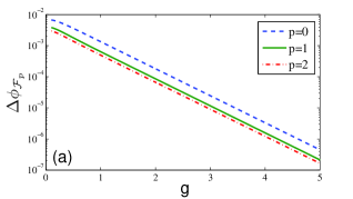
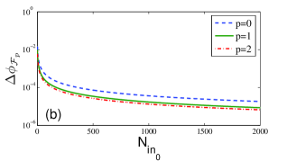
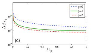
Figure 2: (Color online) The phase sensitivities $\Delta\phi_{\mathcal{F}_{p}}$ of the SU(1,1) interferometer (a) versus $g$ with $N_{\text{in}_{0}}=200$; (b) versus $N_{\text{in}_{0}}$ with $g=3$ where $\eta_{0}=0.5$; (c) versus $\eta_{0}$ with $g=3$ and $N_{\text{in}_{0}}=200$.

As shown in Fig. 1, a BS with low reflectance and a single-photon resolution photo-detector are used to subtract $p$ photons from input squeezed vacuum state. The reflected photons that are detected herald a $p$-photon subtracted squeezed-vacuum state generation Biswas

$$|p,\varsigma\rangle_{b}\sim\hat{b}^{p}|0,\varsigma\rangle_{b},$$ (8)

where $|0,\varsigma\rangle_{b}=\hat{S}_{b}(r)|0\rangle_{b}$ is a single-mode squeezed vacuum state in the $b$-mode, and $\hat{S}_{b}(r)=\exp[(-\varsigma\hat{b}^{{\dagger}2}+\varsigma^{\ast}\hat{b}^{2})/2]$ with $\varsigma=r\exp(i\theta_{\varsigma})$ is the single-mode squeezing parameter. We consider a coherent light combined with a $p$-photon subtracted squeezed vacuum light as input, i.e., $|\Psi_{\text{in}}\rangle=|\alpha\rangle_{a}\otimes|p,\varsigma\rangle_{b}$, where $\alpha=\left|\alpha\right|e^{i\theta_{\alpha}}$. Here, we use this state as the probe state in phase sensitivity measurement. We firstly derive the QFI $\mathcal{F}_{p}$ $(p=0,1,2)$.

For $p=0$, the input state $|\Psi_{\text{in}}\rangle$ is the coherent state $\otimes$ squeezed vacuum state, which has been studied by some of us only with the method of error propagation using the homodyne detection Li14 and parity detection Li16 . For $p=1$ and $p=2$, the $p$-photon subtracted squeezed vacuum states $|p,\varsigma\rangle_{b}$ are respectively given by

$$|1,\varsigma\rangle=\frac{1}{\sqrt{\bar{n}_{0}}}\hat{b}|0,\varsigma\rangle_{b},$$ (9)

and

$$|2,\varsigma\rangle=\frac{1}{\sqrt{\bar{n}_{0}\bar{n}_{1}}}\hat{b}^{2}|0,\varsigma\rangle_{b},$$ (10)

where $\bar{n}_{0}=\sinh^{2}r$ and $\bar{n}_{1}=\sinh^{2}r+\cosh(2r)$. Using the coherent state combined with a $p$-photon subtracted squeezed vacuum state as input ($p=0$, $1$, $2$), when $\theta_{\varsigma}+2\theta_{\alpha}-2\theta_{1}=\pi$, according to Eq. (4) the maximal QFIs of them are given by

$$\mathcal{F}_{0} =\cosh^{2}(2g)\left[\frac{1}{2}\sinh^{2}(2r)+\left|\alpha\right|^{2}\right]+\sinh^{2}(2g)$$

$$\times\left[\left|\alpha\right|^{2}e^{2r}+\bar{n}_{0}+1\right],$$ (11)

$$\mathcal{F}_{1} =\cosh^{2}(2g)\left[\frac{3}{2}\sinh^{2}(2r)+\left|\alpha\right|^{2}\right]+\sinh^{2}(2g)$$

$$\times[3\left|\alpha\right|^{2}e^{2r}+\bar{n}_{1}+1],$$ (12)

$$\mathcal{F}_{2} =\cosh^{2}(2g)[\frac{3}{2}\sinh^{2}(2r)\frac{5\sinh^{2}r(\bar{n}_{1}+1)+3}{\bar{n}_{1}^{2}}$$

$$+\left|\alpha\right|^{2}]+\sinh^{2}(2g)\{\left|\alpha\right|^{2}[3\sinh(2r)\frac{5\sinh^{2}r+1}{\bar{n}_{1}}$$

$$+2\bar{n}_{2}+1]+\bar{n}_{2}+1\},$$ (13)

where $\bar{n}_{2}=3\sinh^{2}r(5\sinh^{2}r+3)/\bar{n}_{1}$. Here $\bar{n}_{p}$ are the mean photon number of $p$-photon subtracted squeezed vacuum states ($p=0$, $1$, $2$). $\mathcal{F}_{0}$ has been studied by some of us Gong16 , and here it is used for comparison with $\mathcal{F}_{1}$ and $\mathcal{F}_{2}$.

Next, we give the QCRB according to the QFI, which is given by

$$\Delta\phi_{\mathcal{F}}=\frac{1}{\sqrt{m\mathcal{F}_{p}}}\text{ \ \ }(p=0\text{, }1\text{, }2),$$ (14)

where $m$ is the number of independent repeats of the experiment, and subscript $p$ denotes subtracting $p$ photons from the squeezed vacuum state. Using Eq. (14) we obtain the phase sensitivities $\Delta\phi_{\mathcal{F}_{p}}$, which increase with increasing $g$ and $N_{\text{in}_{0}}$ as shown in Figs. 2 (a) and (b). For fixed $N_{\text{in}_{0}}$ and $g$, the phase sensitivities $\Delta\phi_{\mathcal{F}_{p}}$ also improve with increasing the photon subtractions $p$ ($p=0$, $1$, $2$). For given a fixed input mean number of photons $N_{\text{in}_{0}}$, the subtraction of photons from the squeezed vacuum state increases the corresponding sensitivity in the phase-shift measurement. Therefore, for the coherent state $\otimes$ the squeezed vacuum state input, given a fixed input mean number of photons $N_{\text{in}_{0}}$, the phase sensitives $\Delta\phi_{\mathcal{F}}$ can be improved by subtracting the photons from the squeezed vacuum state, which seems to conflict with the result of Lang and Caves Lang and we explain it in Sec. IV.

To describe the effect of unbalanced input states on the QFI, we introduce a parameter $\eta_{p}$ which is defined by

$$\eta_{p} \equiv\frac{\text{mean photon number of }b\text{ mode input}}{\text{total mean photon number of input}}$$

$$=\bar{n}_{p}/N_{\text{in}_{p}}\text{ }(p=0,1,2),$$ (15)

where the total mean photon numbers into the first NBS are written as $N_{\text{in}_{p}}=\left|\alpha\right|^{2}+\bar{n}_{p}$ ($p=0$, $1$, $2$). For $p=0$ the squeezed vacuum state with coherent state input, when $\eta_{0}=0$, the input state is a coherent state $|\alpha\rangle$, and when $\eta_{0}=1$, it is a squeezed vacuum state input. For a given fixed $N_{\text{in}_{0}}$, in order to find the dominant component of $r$ and $\left|\alpha\right|$, the phase sensitivities $\Delta\phi_{\mathcal{F}}$ as a function of the squeezing fraction $\eta_{0}$ is shown in Fig. 2(c). We find that the optimal squeezing fraction $\eta_{0}$ is $1$ for a given fixed $N_{\text{in}_{0}}$. That is for a given fixed $N_{\text{in}_{0}}$, only with $p$-photon subtracted squeezed vacuum light as input and without the coherent state, the phase sensitivities are the highest $(p=0,1,2)$.

III Heisenberg limit

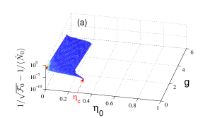
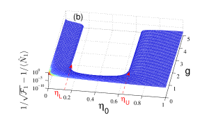
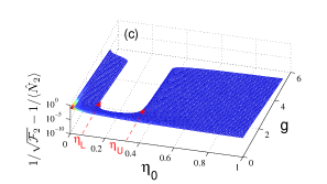
Figure 3: (Color online) Under the condition of small-$m$ case ($m=1$), the difference between the phase sensitivities $\Delta\phi_{\mathcal{F}_{p}}$ $(=1/\sqrt{\mathcal{F}_{p}})$ and HL $\Delta\phi_{\mathrm{HL}_{p}}$ $(=1/\langle\hat{N}_{p}\rangle)$ as a function of $\eta_{0}$ and $g$ with $N_{\mathrm{in}_{0}}=200$ for (a) $p=0$; (b) $p=1$; (c) $p=2$. In the blank areas of $\eta_{\text{0}}>\eta_{c}$ and $\eta_{\text{L}}<\eta_{0}<\eta_{\text{U}}$, the phase sensitivities $\Delta\phi_{\mathcal{F}}$ can beat the the scaling $1/\langle\hat{N}\rangle$ under a certain condition.

The HL is ultimate scaling of the phase sensitivity imposed by quantum mechanics. For the number of particles in the probe state is fixed and is equal to $N$ (without number fluctuations), the fundamental HL is given by pezze2015

$$\Delta\phi_{\text{HL}}=\frac{1}{\sqrt{m}N},$$ (16)

where the factor $m$ is the number of independent measurements repeated with identical copies of the probe state. In the SU(2) scheme, the optimal input state is the NOON state and the sensitivity is $1/N$ NOON ; Dowling . However, for a fixed mean photon number (with number fluctuations) the form of the HL has been questioned Sharpio ; Pasquale . Considering the photon number fluctuations, Hofmann suggested the form of HL is $1/\langle\hat{N}^{2}\rangle^{1/2}$, where indicates averaging over the squared photon numbers hofmann . But the phase sensitivity can be arbitrary high for large fluctuations. For separable state and with unbiased phase estimators, Pezzè et al. pointed out that the HL for two-mode interferometers should add extra constraints and is given by pezze2015 ; hyllus

$$\Delta\phi_{\text{HL}}=\max\left[\frac{1}{\sqrt{m\langle\hat{N}^{2}\rangle}},\frac{1}{m\langle\hat{N}\rangle}\right],\text{ for }\langle\Delta\hat{N}\rangle>0.$$ (17)

Eq. (17) cannot be obtained from Eq. (16) by simply replacing $N$ with $\langle\hat{N}\rangle$. But Eq. (17) can reduce to Eq. (16) when number fluctuations vanish, i.e., $\langle\hat{N}^{2}\rangle=\langle\hat{N}\rangle^{2}=N^{2}$.

For the SU (1,1) interferometer, $\langle\hat{N}\rangle$ $(\equiv\langle\Psi|\hat{n}_{a}+\hat{n}_{b}|\Psi\rangle)$ is the total number of photons inside the interferometer Marino , not the input one as the traditional MZI. This is due to phase sensing by the total photons of the two modes inside the interferometer. The mean photon numbers inside the interferometer for $p=0$, $1$ and $2$ are respectively given by

$$\langle\hat{N}_{p}\rangle=\cosh(2g)N_{\text{in}_{p}}+2\sinh^{2}(g),\text{ }(p=0,1,2).$$ (18)

Similarly, one can obtain the squared photon numbers inside the SU(1,1) interferometer, which are given as following:

$$\langle\hat{N}_{0}^{2}\rangle =\left(\left|\alpha\right|^{4}+3\bar{n}_{0}^{2}\right)\cosh^{2}(2g)+4\left(N_{\text{in}_{0}}+1\right)\sinh^{4}(g)$$

$$+[\left|\alpha\right|^{2}\cosh(2r)+2\bar{n}_{0}]\cosh(4g)+\sinh^{2}(2g)$$

$$\times[\left|\alpha\right|^{2}(\sinh(2r)+1)+1],$$ (19)

$$\langle\hat{N}_{1}^{2}\rangle =\cosh(4g)[\left|\alpha\right|^{2}(6\bar{n}_{0}+1)+2N_{\text{in}_{1}}-1]+\cosh^{2}(2g)$$

$$\times(15\bar{n}_{0}^{2}+\left|\alpha\right|^{4}+6\bar{n}_{0})+4\sinh^{4}g(N_{\text{in}_{1}}+1)$$

$$+\sinh^{2}(2g)[\left|\alpha\right|^{2}+2+3\left|\alpha\right|^{2}\sinh(2r)],$$ (20)

$$\langle\hat{N}_{2}^{2}\rangle=\cosh(4g)[2\bar{n}_{2}+\left|\alpha\right|^{2}(2\bar{n}_{2}+1)]+4\sinh^{4}(g)(1$$

$$+N_{\text{in}_{2}})+\cosh^{2}(2g)\left[35\bar{n}_{0}^{2}+\frac{1}{3\bar{n}_{0}+1}40\bar{n}_{0}^{2}+\left|\alpha\right|^{4}\right]$$

$$+\sinh^{2}(2g)\left[\left|\alpha\right|^{2}+3\frac{5\bar{n}_{0}+1}{3\bar{n}_{0}+1}\left|\alpha\right|^{2}\sinh 2r+1\right],$$ (21)

where $\theta_{\varsigma}+\theta_{\alpha}-\theta_{1}=\pi$.

Next, we compare the QCRB with the HL from Eq. (17). According to the number of measurements $m$, we study two cases: (i) small-$m$ case; (ii) large-$m$ case. As discussed in Ref. pezze2015 , in the limit of small-$m$ the HL of Eq. (17) is found to be

$$\Delta\phi_{\text{HL}p}=\frac{1}{m\langle\hat{N}_{p}\rangle}\text{ \ }(p=0\text{, }1\text{, }2).$$ (22)

In this situation, we consider $m=1$, and the HLs are given by

$$\Delta\phi_{\text{HL}p}=\frac{1}{\langle\hat{N}_{p}\rangle}\text{ \ \ }(p=0\text{, }1\text{, }2).$$ (23)

For a given input number, the difference between the phase sensitivity $\Delta\phi_{\mathcal{F}_{p}}$ and the HL $\Delta\phi_{\text{HL}p}$ ($p=0$, $1$, $2$) as a function of $\eta_{0}$ and $g$ is shown in Fig. 3. When $\eta_{\text{0}}>\eta_{c}$ and $\eta_{\text{L}}<\eta_{0}<\eta_{\text{U}}$, the phase sensitivities $\Delta\phi_{\mathcal{F}_{p}}$ can beat the the scaling $1/\langle\hat{N}_{p}\rangle$ ($\Delta\phi_{\mathcal{F}_{p}}-$ $\Delta\phi_{\text{HL}p}<0$, $p=0$, $1$, $2$) within certain parameters, as shown in the blank areas of Fig. 3. For $p=$ $1\$and $2$ cases, with a given $N_{\text{in}_{0}}$ and $g$, although the phase sensitivities $\Delta\phi_{\mathcal{F}}$ are optimal under the condition of $\eta_{0}=1$ shown in Fig. 2(c), the areas of $\Delta\phi_{\mathcal{F}_{p}}-$ $\Delta\phi_{\text{HL}p}<0$ is $\eta_{\text{L}}<\eta_{0}<\eta_{\text{U}}$ as shown in Fig. 3(b) and (c). The reason is that both the phase sensitivity $\Delta\phi_{\mathcal{F}}$ and the HL $\Delta\phi_{\text{HL}}$ enhance with increase of $\eta_{0}$, but the increasing rate of $\Delta\phi_{\text{HL}}$ is higher.

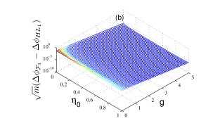
Figure 4: (Color online) Under the condition of large-$m$ case, the difference between the phase sensitivities $\Delta\phi_{\mathcal{F}_{p}}$ $(=1/\sqrt{m\mathcal{F}_{p}})$ and HL $\Delta\phi_{\mathrm{HL}_{p}}$ $(=1/\sqrt{m\langle\hat{N}_{p}^{2}\rangle})$ as a function of $\eta_{0}$ and $g$ with $N_{\mathrm{in}_{0}}=200$ for (a) $p=0$; (b) $p=1$; (c) $p=2$.

Now we will study the case of large-$m$ limit. As shown in Ref. pezze2015 , the HL of Eq. (17) in the large-$m$ limit is given by

$$\Delta\phi_{\text{HL}p}=\frac{1}{\sqrt{m\langle\hat{N}_{p}^{2}\rangle}}\text{ \ \ }(p=0\text{, }1\text{, }2).$$ (24)

We compare the corresponding HL of Eq. (24) with the phase sensitivity by QCRB in Figs. 4(a)-(c) under various input situations, and obtain that the HL of large-$m$ limit case cannot be beaten.

The comparison between two different results shown in Figs. 3 and 4 deserves a discussion. In the small-$m$ limit ($m=1$ particularly), for the $p$-photon subtracted squeezed vacuum states input the phase sensitivity QCRB $\Delta\phi_{\mathcal{F}_{p}}=1/\sqrt{\mathcal{F}_{p}}$ can beat $1/\langle\hat{N}_{p}\rangle$. While in the large-$m$ limit, this ultimate quantum limit of SU(1,1) interferometer is $\Delta\phi_{\text{HL}p}=1/\sqrt{m\langle\hat{N}_{p}^{2}\rangle}$, and it cannot be beaten. As we all know, the HL is as the maximum sensitivity achievable, optimized over all possible estimators, measurements and probe states. However, in presence of large fluctuations in the number of probes, the violation of $1/\langle\hat{N}\rangle$ scaling of the optimal accuracy is possible Sharpio ; Pasquale , and the definition of the HL should take into account the amount of fluctuations hofmann ; pezze2015 . Hence, this HL $\Delta\phi_{\text{HL}p}=1/\sqrt{m\langle\hat{N}_{p}^{2}\rangle}$ considering the number fluctuation effect could be the ultimate phase sensitivity limit hofmann ; hyllus ; pezze2015 .

IV Discussion

Figure 5: (Color online) The phase sensitivities $\Delta\phi_{\mathcal{F}_{p}}$ as a function of $\eta_{p}$ $(p=0,1,2)$ with $N_{\text{in}_{0}}=N_{\text{in}_{1}}=N_{\text{in}_{2}}=200$ and $g=3$.

For the coherent state $\otimes$ the squeezed vacuum state input, given a fixed input mean number of photons $N_{\text{in}_{0}}$, the phase sensitives $\Delta\phi_{\mathcal{F}}$ can be improved by subtracting the photons from the squeezed vacuum state, as shown in Fig. 2. That is within the constraint on the average photon of a squeezed vacuum state, it is still possible to attain higher sensitivity via photon subtraction. It seems to conflict with the result of proposal presented by Lang and Caves Lang . They considered that an interferometer powered by laser light (a coherent state) into one input port and ask the following question: what is the best state to inject into the second input port, given a constraint on the mean number of photons this state can carry, in order to optimize the interferometer’s phase sensitivity? Their answer is squeezed vacuum. In fact, they don’t conflict and the reason is given as follows.

With $N_{\text{in}_{p}}$ and $\eta_{p}$, the maximal QFIs $\mathcal{F}_{p}$ ($p=0$, $1$, $2$) are rewritten as

$$\mathcal{F}_{0} =\cosh^{2}(2g)[\eta_{0}N_{\text{in}_{0}}(1+2\eta_{0}N_{\text{in}_{0}})+N_{\text{in}_{0}}]+\sinh^{2}(2g)$$

$$\times[2\eta_{0}(1-\eta_{0})(N_{\text{in}_{0}})^{2}+2\sqrt{\eta_{0}N_{\text{in}_{0}}(\eta_{0}N_{\text{in}_{0}}+1)}$$

$$\times(1-\eta_{0})N_{\text{in}_{0}}+N_{\text{in}_{0}}+1],$$ (25)

$$\mathcal{F}_{1} =\cosh^{2}(2g)[\frac{2}{3}(\eta_{1}N_{\text{in}_{1}}-1)(\eta_{1}N_{\text{in}_{1}}+2)+(1-\eta_{1})$$

$$\times N_{\text{in}_{1}}]+\sinh^{2}(2g)[2\eta_{1}(N_{\text{in}_{1}})^{2}(1-\eta_{1})+N_{\text{in}_{1}}+1$$

$$+2N_{\text{in}_{1}}(1-\eta_{1})\sqrt{(\eta_{1}N_{\text{in}_{1}}-1)(\eta_{1}N_{\text{in}_{1}}+2)}],$$ (26)

$$\mathcal{F}_{2} =\cosh^{2}(2g)[6S(S+1)\frac{5S(3S+2)+3}{(3S+1)^{2}}+(1-\eta_{2})$$

$$\times N_{\text{in}_{2}}]+\sinh^{2}(2g)\{N_{\text{in}_{2}}(1-\eta_{2})[6\sqrt{S(S+1)}$$

$$\times\frac{5S+1}{3S+1}+2\eta_{2}N_{\text{in}_{2}}+1]+\eta_{2}N_{\text{in}_{2}}+1\},$$ (27)

where

$$S=\frac{\eta_{2}N_{\text{in}_{2}}-3+\sqrt{\left(\eta_{2}N_{\text{in}_{2}}\right)^{2}+\frac{2}{3}\eta_{2}N_{\text{in}_{2}}+9}}{10}.$$ (28)

Let $N_{\text{in}_{0}}=N_{\text{in}_{1}}=N_{\text{in}_{2}}$ and for a fixed $g$, the phase sensitivities $\Delta\phi_{\mathcal{F}_{p}}$ as a function of the squeezing fraction $\eta_{p}$ is shown in Fig. 5, and we obtain $\Delta\phi_{\mathcal{F}_{0}}<\Delta\phi_{\mathcal{F}_{1}}<\Delta\phi_{\mathcal{F}_{2}}$. which agrees with the result given by Lang and Caves Lang . However, the reflected photons that are detected herald a photon-subtracted squeezed-vacuum state generation, the sensitivity of phase-shift estimation can also be improved. The generation process of photon-subtracted squeezed-vacuum state need to use additional resources and is probability.

V Conclusions

We have studied the phase sensitivities of an SU(1,1) interferometer with a coherent state in one input port and a photon-subtracted squeezed vacuum state in the other input port using QCRB. The subtraction of photons from the squeezed vacuum state not only increases the average photon number for the fixed squeezed parameter $r$, but also increases the corresponding sensitivity in the phase-shift measurement. The HL considering the number fluctuation effect cannot be beaten and may be the ultimate phase limit. The enhancement of phase sensitivity with nonclassical light is dominant from the intramode correlations, hence the mode entanglement is not a critical resource for quantum metrology. Using separable states have many advantages over entangled states including more flexibility in the distribution of resources, comparatively easier state preparation.

References

- (1) J. H. Shapiro, S. R. Shepard, and N. C. Wong, Ultimate quantum limits on phase measurement, Phys. Rev. Lett. 62, 2377 (1989).
- (2) A. D. Pasquale, P. Facchi, G. Florio, V. Giovannetti, K. Matsuoka, and K. Yuasa, Two-mode bosonic quantum metrology with number fluctuations, Phys. Rev. A 92, 042115 (2015).
- (3) H. F. Hofmann, All path-symmetric pure states achieve their maximal phase sensitivity in conventional two-path interferometry, Phys. Rev. A 79, 033822 (2009).
- (4) P. Hyllus, L. Pezzé, and A. Smerzi, Entanglement and Sensitivity in Precision Measurements with States of a Fluctuating Number of Particles, Phys. Rev. Lett. 105, 120501 (2010).
- (5) L. Pezzè, P. Hyllus, and A. Smerzi, Phase-sensitivity bounds for two-mode interferometers, Phys. Rev. A 91, 032103 (2015).
- (6) C. W. Helstrom, Quantum Detection and Estimation Theory (Academic, New York, 1976).
- (7) A. S. Holevo, Probabilistic and Statistical Aspects of Quantum Theory (North-Holland, Amsterdam, 1982).
- (8) C. M. Caves, Quantum-mechanical noise in an interferometer, Phys. Rev. D 23, 1693(1981)
- (9) S. L. Braunstein and C. M. Caves, Statistical distance and the geometry of quantum states, Phys. Rev. Lett. 72, 3439 (1994).
- (10) S. L. Braunstein, C. M. Caves, and G. J. Milburn, Generalized uncertainty relations: Theory, examples, and Lorentz invariance, Ann. Phys. 247, 135 (1996).
- (11) H. Lee, P. Kok, and J. P. Dowling, J Mod, A quantum Rosetta stone for interferometry, Opt 49, 2325 (2002).
- (12) V. Giovannetti, S. Lloyd, and L. Maccone, Quantum Metrology, Phys. Rev. Lett. 96, 010401 (2006).
- (13) M. Zwierz, C. A. Pérez-Delgado, and P. Kok, General Optimality of the Heisenberg Limit for Quantum Metrology, Phys. Rev. Lett. 105, 180402 (2010).
- (14) V. Giovannetti, S. Lloyd, and L. Maccone, Quantum-Enhanced Measurements: Beating the Standard Quantum Limit, Science 306, 1330 (2004).
- (15) V. Giovannetti, S. Lloyd, and L. Maccone, Advances in quantum metrology, Nature photonics 5, 222 (2011).
- (16) B. P. Abbott et al. (LIGO Scientific Collaboration and Virgo Collaboration), Observation of Gravitational Waves from a Binary Black Hole Merger, Phys. Rev. Lett. 116, 061102 (2016).
- (17) G. Tóth and I. Apellaniz, Quantum metrology from a quantum information science perspective, J. Phys. A 47, 424006 (2014).
- (18) J. Sahota and N. Quesada, Quantum correlations in optical metrology: Heisenberg-limited phase estimation without mode entanglement, Phys. Rev. A 91, 013808 (2015).
- (19) A. N. Boto, P. Kok, D. S. Abrams,S. L. Braunstein, C. P. Williams, and J. P. Dowling, Quantum Interferometric Optical Lithography: Exploiting Entanglement to Beat the Diffraction Limit, Phys. Rev. Lett. 85, 2733 (2000).
- (20) J. P. Dowling, Quantum optical metrology-the lowdown on high-NOON states, Contemp. Phys. 49, 125 (2008).
- (21) P. A. Knott, T. J. Proctor, A. J. Hayes, J. P. Cooling, and J. A. Dunningham, Practical quantum metrology with large precision gains in the low-photon-number regime, Phys. Rev. A 93, 033859 (2016).
- (22) K. Berrada and S. A. Khalek, Quantum phase estimation for nonlinear phase shifts with entangled spin coherent states of two modes, Laser Phys. 23, 105201 (2013).
- (23) B. Yurke, S. L. McCall, and J. R. Klauder, SU(2) and SU(1,1) interferometers, Phys. Rev. A 33, 4033 (1986).
- (24) W. N. Plick, J. P. Dowling, and G. S. Agarwal, Coherent-light-boosted, sub-shot noise, quantum interferometry, New J. Phys. 12, 083014 (2010).
- (25) D. Li, C.-H. Yuan, Z. Y. Ou, and W. Zhang, The phase sensitivity of an SU (1, 1) interferometer with coherent and squeezed-vacuum light, New J. Phys. 16, 073020 (2014).
- (26) J. Jing, C. Liu, Z. Zhou, Z. Y. Ou, and W. Zhang, Realization of a nonlinear interferometer with parametric amplifiers, Appl. Phys. Lett. 99, 011110 (2011).
- (27) Z. Y. Ou, Enhancement of the phase-measurement sensitivity beyond the standard quantum limit by a nonlinear interferometer, Phys. Rev. A 85, 023815 (2012).
- (28) A. M. Marino, N. V. Corzo Trejo, and P. D. Lett, Effect of losses on the performance of an SU(1,1) interferometer, Phys. Rev. A 86, 023844 (2012).
- (29) F. Hudelist, J. Kong, C. Liu, J. Jing, Z. Y. Ou, and W. Zhang, Quantum metrology with parametric amplifier-based photon correlation interferometers, Nat. Commun. 5, 3049 (2014).
- (30) C. Gross, T. Zibold, E. Nicklas, J. Estève, and M. K. Oberthaler, Nonlinear atom interferometer surpasses classical precision limit, Nature (London) 464, 1165 (2010).
- (31) D. Linnemann, Realization of an SU(1,1) Interferometer with Spinor Bose-Einstein Condensates (Master thesis, University of Heidelberg, 2013).
- (32) J. Peise, B. Lücke, L. Pezzè, F. Deuretzbacher, W. Ertmer, J. Arlt, A. Smerzi, L. Santos, and C. Klempt, Interaction-free measurements by quantum Zeno stabilization of ultracold atoms, Nat. Commun. 6, 6811 (2015).
- (33) M. Gabbrielli, L. Pezzè, and A. Smerzi, Spin-Mixing Interferometry with Bose-Einstein Condensates, Phys. Rev. Lett. 115, 163002 (2015).
- (34) B. Chen, C. Qiu, S. Chen, J. Guo, L. Q. Chen, Z. Y. Ou, and W. Zhang, Atom-Light Hybrid Interferometer, Phys. Rev. Lett. 115, 043602 (2015).
- (35) J. Jacobson, G. Björk, and Y. Yamamoto, Quantum limit for the atom-light interferometer, Appl. Phys. B 60, 187-191 (1995).
- (36) S. A. Haine, Quantum Metrology in Open Systems: Dissipative Cramer-Rao Bound, Phys. Rev. Lett. 112, 120405 (2014).
- (37) S. S. Szigeti, B. Tonekaboni, W. Y. S. Lau, S. N. Hood, and S. A. Haine, Squeezed-light-enhanced atom interferometry below the standard quantum limit, Phys. Rev. A 90, 063630 (2014).
- (38) S. A. Haine and W. Y. S. Lau, Generation of atom-light entanglement in an optical cavity for quantum enhanced atom interferometry, Phys. Rev. A 93, 023607 (2016).
- (39) Z.-D. Chen, C.-H. Yuan, H.-M. Ma, D. Li, L. Q. Chen, Z. Y. Ou, and W. Zhang, Effects of losses in the atom-light hybrid SU(1,1) interferometer, Opt. Express 24, 17766 (2016).
- (40) Sh. Barzanjeh, D. P. DiVincenzo and B. M. Terhal, Dispersive qubit measurement by interferometry with parametric amplifiers, Phys. Rev. B 90, 134515 (2014).
- (41) M. D. Lang and C. M. Caves, Optimal Quantum-Enhanced Interferometry Using a Laser Power Source, Phys. Rev. Lett. 111, 173601 (2013).
- (42) A. Biswas and G. S. Agarwal, Nonclassicality and decoherence of photon-subtracted squeezed states, Phys. Rev. A 75, 032104 (2007).
- (43) R. Birrittella and C. C. Gerry, Quantum optical interferometry via the mixing of coherent and photon-subtracted squeezed vacuum states of light, J. Opt. Soc. Am. B 31, 586 (2014).
- (44) M. Ueda, N. Imoto, and T. Ogawa, Quantum theory for continuous photodetection processes, Phys. Rev. A 41, 3891–3904 (1990).
- (45) S. S. Mizrahi and V. V. Dodonov, Creating quanta with an “annihilation” operator, J. Phys. A 35, 8847–8857 (2002).
- (46) L. Mandel and E. Wolf, Optical coherent and quantum optics (Cambridge University Press, 1955).
- (47) M. Dakna, T. Anhut, T. Opatrný, L. Knöll, and D.-G. Welsch, Generating Schröinger-cat-like states by means of conditional measurements on a beam splitter, Phys. Rev. A 55, 3184 (1997).
- (48) M. Takeola, H. Takahashi, and M. Sasaki, Large-amplitude coherent-state superpositions generated by a time-separated two-photon subtraction from a continuous-wave squeezed vacuum, Phys. Rev. A 77, 062315 (2008).
- (49) A. Ourjoumtsev, R. Tualle-Brouri, J. Laurat, and P. Grangier, Generating Optical Schrödinger Kittens for Quantum Information Processing, Science 312, 83 (2006).
- (50) K. Wakui, H. Takahashi, A. Furusawa, and M. Sasaki, Photon subtracted squeezed states generated with periodically poled KTiOPO4, Opt. Express 15, 3568 (2007).
- (51) N. Namekata, Y. Takahashi, G. Fuji, D. Fukuda, S. Kurimura, and S. Inoue, Non-Gaussian operation based on photon subtraction using a photon-number-resolving detector at a telecommunications wavelength, Nature Photon. 4, 655 (2010).
- (52) T. Gerrits, S. Glancy, T. S. Clement, B. Calkins, A. E. Lita, A. J. Miller, A. L. Migdall, S. W. Nam, R. P. Mirin, and E. Knill, Generation of optical coherent-state superpositions by number-resolved photon subtraction from the squeezed vacuum, Phys. Rev. A 82, 031802(R) (2010).
- (53) L. Pezzè and A. Smerzi, in Proceedings of the International School of Physics “Enrico Fermi”, Course CLXXXVIII “Atom Interferometry” edited by G. Tino and M. Kasevich (Società Italiana di Fisica and IOS Press, Bologna, 2014), p. 691-741.
- (54) Two Hermitian operators and generate the two-mode squeezing operator , where is the squeezed parameter of the nonlinear beam splitter.
- (55) P. Kok and B. W. Lovett, Introduction to optical quantum information processing, (Cambridge University Press, 2010).
- (56) M. Jarzyna and R. Demkowicz-Dorbrzanski, Quantum interferometry with and without an external phase reference, Phys. Rev. A 85, 011801(R) (2012).
- (57) C. C. Gerry and P. L. Knight, Introductory Quantum Optics (Cambridge University Press, 2005).
- (58) J. Sahota, N. Quesada, and D. F. V. James, Physical Resources for Quantum-enhanced Phase Estimation, arXiv:1603.02375
- (59) D. Li, B. T. Gard, Y. Gao, C.-H. Yuan, W. Zhang, H. Lee, and J. P. Dowling, Phase sensitivity at the Heisenberg limit in an SU(1,1) interferometer via parity detection, arXiv:1603.09019
- (60) Q.-K. Gong, D. Li, C.-H. Yuan, Z. Y. Ou, and W. Zhang, Bounds to precision for an SU(1,1) interferometer with Gaussian input states, arXiv:1608.00389