Disciplined Multi-Convex Programming

Abstract

A multi-convex optimization problem is one in which the variables can be partitioned into sets over which the problem is convex when the other variables are fixed. Multi-convex problems are generally solved approximately using variations on alternating or cyclic minimization. Multi-convex problems arise in many applications, such as nonnegative matrix factorization, generalized low rank models, and structured control synthesis, to name just a few. In most applications to date the multi-convexity is simple to verify by hand. In this paper we study the automatic detection and verification of multi-convexity using the ideas of disciplined convex programming. We describe an implementation of our proposed method that detects and verifies multi-convexity, and then invokes one of the general solution methods.

1 Introduction

A multi-convex optimization problem is one in which the variables can be partitioned into sets over which the problem is convex when the other variables are fixed. Multi-convex problems appear in domains such as machine learning [lee1999learning, udell2014generalized], signal and information processing [Lee00, Kim2008, Wen2012], communication [1254038], and control [751690, hassibi1999path, hours2014parametric, 7170815]. Typical problems in these fields include nonnegative matrix factorization (NMF) and bilinear matrix inequality (BMI) problems.

In general multi-convex problems are hard to solve globally, but several algorithms have been proposed as heuristic or local methods, and are widely used in applications. Most of these methods are variations on the block coordinate descent (BCD) method. The idea of optimizing over a single block of variables while holding the remaining variables fixed in each iteration dates back to [Warga, Powell1973]. Convergence results were first discussed for strongly convex differentiable objective function [Warga], and then under various assumptions on the separability and regularity of the objective function [Tseng1993, Tseng2001]. In [attouch2010], a two-block BCD method with proximal operator is used to minimize a nonconvex objective function which satisfies the Kurdyka-Lojasiewicz inequality. In [razaviyayn2012unified] the authors propose an inexact BCD approach which updates variable blocks by minimizing a sequence of approximations of the objective function, which can either be nondifferentiable or nonconvex. A recent work [xu2013block] uses BCD to solve multi-convex problems, where the objective is a sum of a differentiable multi-convex function and several extended-valued convex functions. In each step, updates with and without proximal operator and prox-linear operator are considered, and convergence analysis is established under certain assumptions. Gradient methods have also been proposed for multi-convex problems, where the objective is differentiable in each block of variables, and all variables are updated at once along their descent directions and then projected into a convex feasible set in every iteration [Chu04].

The focus of this paper is not on solution methods, but on a modeling framework for expressing multi-convex problems in a way that verifies the multi-convex structure, and can expose the structure to whatever solution algorithm is then used. Modeling frameworks have been developed for convex problems, e.g., CVX [cvx], YALMIP [Lofberg:04], CVXPY [cvxpy_paper], and Convex.jl [cvxjl]. These frameworks provide a uniform method for specifying convex problems based on the idea of disciplined convex programming (DCP) [GBY:06]. This gives a simple method for verifying that a problem is convex, and for automatically canonicalizing to a standard generic form such as a cone program. The goal of DCP (and these software frameworks) is not to detect or determine feasibility of an arbitrary problem, but rather to give a very simple set of rules that can be used to construct convex problems.

In this paper we extend the idea of DCP to multi-convex problems. We propose a disciplined multi-convex programming (DMCP) rule set, an extension of the DCP rule set. Problem specifications that conform to the DMCP rule set can be verified as convex in a group of variables, for any fixed values of the other variables, using ideas that extend those in DCP. We describe an efficient algorithm that can carry out the analysis of convexity of problem when an arbitrary group of variables is fixed at any value. As with DCP, the goal of DMCP is not to analyze multi-convexity of an arbitrary problem, but rather to give a simple set of rules which if followed yields multi-convex problems. In applications to date, such as NMF, verification of multi-convexity is simple, and can be done by hand or just simple observation. With DMCP a far larger class of multi-convex problems can be constructed in an organized way.

We describe a software implementation of the ideas developed in this paper, called DMCP, a Python package that extends CVXPY. It implements the DMCP verification and analysis methods, and then heuristically solves a conforming problem via BCD type algorithms, which we extend for general use to include slack variables to handle infeasibility. A similar package, MultiConvex, has been developed for the Julia package Convex.jl. We illustrate the framework on a number of examples.

In §2 we carefully define multi-convexity of a function, constraint, and problem. We review block coordinate descent methods, introducing new variants with slack variables and generalized inequalities, in §3. In §4 we describe the main ideas of DMCP and an efficient algorithm for verifying that a problem specification conforms to DMCP. In §5 we describe our implementation of the package DMCP. Finally, in §6 we describe a number of numerical examples. Our goal there is not to show competitive results, in terms of solution quality or solve time, but rather to show the simplicity with which the problem is specified, along with results that are at least comparable to those obtained with custom solvers for the specific problem.

2 Multi-convex programming

2.1 Multi-convex function

Fixing variables in a function.

Consider a function $f:{\mbox{\bf R}}^{n}\to{\mbox{\bf R}}\cup\{\infty\}$, and a partition of the variable $x\in{\mbox{\bf R}}^{n}$ into blocks of variables

$$x=(x_{1},\ldots,x_{N}),\quad x_{i}\in{\mbox{\bf R}}^{n_{i}},$$

so $\sum_{i=1}^{N}n_{i}=n$. Throughout this paper we will use subsets of indices to refer to sets of the variables. Let $\mathcal{F}\subseteq\{1,\ldots,N\}$ denote an index set, with complement $\mathcal{F}^{c}=\{1,\ldots,N\}\setminus\mathcal{F}$. By fixing the variables with indices in $\mathcal{F}$ of the function $f$ at a given point $\hat{x}\in{\mbox{\bf R}}^{n}$, we obtain a function over the remaining variables, with indices in $\mathcal{F}^{c}$, which we denote as $\tilde{f}=\mathrm{fix}(f,\hat{x},\mathcal{F})$. For $i\in\mathcal{F}^{c}$, $x_{i}$ is a variable of the function $\tilde{f}$; for $i\in\mathcal{F}$, $x_{i}=\hat{x}_{i}$. Informally we refer to $\tilde{f}$ as ‘$f$, with the variables $x_{i}$ for $i\in\mathcal{F}$ fixed’.

As an example consider $f:{\mbox{\bf R}}^{4}\to{\mbox{\bf R}}\cup\{\infty\}$ defined as

$$f(x_{1},x_{2},x_{3},x_{4})=|x_{1}x_{2}+x_{3}x_{4}|.$$ (1)

With $\hat{x}=(1,2,1,3)$ and $\mathcal{F}=\{1,3\}$, the fixed function $\tilde{f}=\mathrm{fix}(f,\hat{x},\{1,3\})$ is given by $\tilde{f}(x_{2},x_{4})=|x_{2}+x_{4}|$.

Multi-convex and multi-affine functions.

Given an index set $\mathcal{F}\subseteq\{1,\ldots,N\}$, we say that a function $f:{\mbox{\bf R}}^{n}\to{\mbox{\bf R}}\cup\{\infty\}$ is convex (or affine) with set $\mathcal{F}$ fixed, if for any $\hat{x}\in{\mbox{\bf R}}^{n}$ the function $\mathrm{fix}(f,\hat{x},\mathcal{F})$ is a convex (or affine) function. (In this definition, we consider a so-called improper function [rockafellar], which has the value $\infty$ everywhere, as convex or affine.) For example, the function $f$ defined in (1) is convex with the variables $x_{1}$ and $x_{3}$ fixed (i.e., with index set $\mathcal{F}=\{1,3\}$). A function is convex if and only if it is convex with $\mathcal{F}=\emptyset$ fixed, i.e., with none of its variables fixed.

We say the function $f$ is multi-convex (or multi-affine), if there are index sets $\mathcal{F}_{1},\ldots,\mathcal{F}_{K}$, such that for every $k$ the function $f$ is convex (or affine) with $\mathcal{F}_{k}$ fixed, and $\cap_{k=1}^{K}\mathcal{F}_{k}=\emptyset$. The requirement that $\cap_{k=1}^{K}\mathcal{F}_{k}=\emptyset$ means that for every variable $x_{i}$ there is some $\mathcal{F}_{k}$ with $i\not\in\mathcal{F}_{k}$. In particular, $\tilde{f}=\mathrm{fix}(f,\hat{x},\{1,\ldots,N\}\setminus\{i\})$ is convex in $x_{i}$. For $K=2$, we say that the function is bi-convex (or bi-affine).

As an example, the function $f$ in (1) is convex with $\{1,3\}$ fixed and $\{2,4\}$ fixed, so it is multi-convex. The choice of $K$, and the index sets, is not unique. The function $f$ is also convex with $\{2,3,4\}$ fixed, $\{1,3,4\}$ fixed, $\{1,2,4\}$ fixed, and $\{1,2,3\}$ fixed.

Minimal fixed sets.

For a function $f$, we can consider the set of all index sets $\mathcal{F}$ for which $\mathrm{fix}(f,\hat{x},\mathcal{F})$ is convex for all $\hat{x}$; among these we are interested in the minimal fixed sets that render a function convex. A minimal fixed set is a set of variables that when fixed make the function convex; but if any variable is removed from the set, the function is not convex. A function is multi-convex if and only if the intersection of these minimal fixed index sets is empty.

2.2 Multi-convex problem

We now extend the idea of multi-convexity to the optimization problem

$$\begin{array}[]{ll}\mbox{minimize}&f_{0}(x)\\ \mbox{subject to}&f_{i}(x)\leq 0,\quad i=1,\ldots,m\\ &g_{i}(x)=0,\quad i=1,\ldots,p,\end{array}$$ (2)

with variable $x\in{\mbox{\bf R}}^{n}$ partitioned into blocks as $x=(x_{1},\ldots,x_{N})$, and functions $f_{i}:{\mbox{\bf R}}^{n}\to{\mbox{\bf R}}\cup\{\infty\}$ for $i=0,\ldots,m$ and $g_{i}:{\mbox{\bf R}}^{n}\to{\mbox{\bf R}}$ for $i=1,\ldots,p$ are proper.

Given an index set $\mathcal{F}\subseteq\{1,\ldots,N\}$, problem (2) is convex with set $\mathcal{F}$ fixed, if for any $\hat{x}\in{\mbox{\bf R}}^{n}$ the problem

$$\begin{array}[]{ll}\mbox{minimize}&\mathrm{fix}(f_{0},\hat{x},\mathcal{F})\\ \mbox{subject to}&\mathrm{fix}(f_{i},\hat{x},\mathcal{F})\leq 0,\quad i=1,\ldots,m\\ &\mathrm{fix}(g_{i},\hat{x},\mathcal{F})=0,\quad i=1,\ldots,p,\end{array}$$ (3)

is convex. In other words, problem (2) is convex with $\mathcal{F}$ fixed, if and only if functions $f_{i}$ for $i=0,\ldots,m$ are convex with $\mathcal{F}$ fixed, and functions $g_{i}$ for $i=1,\ldots,p$ are affine with $\mathcal{F}$ fixed.

We say the problem (2) is multi-convex, if there are sets $\mathcal{F}_{1},\ldots,\mathcal{F}_{K}$, such that for every $k$ problem (2) is convex with set $\mathcal{F}_{k}$ fixed, and $\cap_{k=1}^{K}\mathcal{F}_{k}=\emptyset$. A convex problem is multi-convex with $K=0$ (i.e., $\mathcal{F}=\emptyset$). A bi-convex problem is multi-convex with $K=2$.

As an example the following problem is multi-convex:

$$\begin{array}[]{ll}\mbox{minimize}&|x_{1}x_{2}+x_{3}x_{4}|\\ \mbox{subject to}&x_{1}+x_{2}+x_{3}+x_{4}=1,\end{array}$$ (4)

with variable $x\in{\mbox{\bf R}}^{4}$. This is readily verfied with $\mathcal{F}_{1}=\{1,3\}$ and $\mathcal{F}_{2}=\{2,4\}$. For a given problem we can consider the minimal variable index sets which make the problem convex. If the problem is convex, $\mathcal{F}=\emptyset$ is the unique minimal set.

3 Block coordinate descent and variations

In this section we review, and extend, some generic methods for approximately solving the multi-convex problem (2), using BCD-type methods.

3.1 Block coordinate minimization with slack variables

Assume that sets $\mathcal{F}_{k}$, $k=1,\ldots,K$ are index sets for which the problem (2) with $\mathcal{F}_{k}$ fixed is convex, with $\cap_{k=1}^{K}\mathcal{F}_{k}=\emptyset$. These could be the set of all minimal index sets, but any other set of index sets that verify multi-convexity could be used.

The basic form of the proposed method is iterative. In each iteration, we fix the variables in one set $\mathcal{F}_{k}$ and solve the following subproblem,

$$\begin{array}[]{ll}\mbox{minimize}&\mathrm{fix}(f_{0},\hat{x},\mathcal{F}_{k})+\mu\sum_{i=1}^{m}s_{i}+\mu\sum_{i=1}^{p}|s_{i+m}|\\ \mbox{subject to}&\mathrm{fix}(f_{i},\hat{x},\mathcal{F}_{k})\leq s_{i},\quad s_{i}\geq 0,\quad i=1,\ldots,m\\ &\mathrm{fix}(g_{i},\hat{x},\mathcal{F}_{k})=s_{i+m},\quad i=1,\ldots,p,\\ \end{array}$$ (5)

where $s_{i}$ for $i=1,\ldots,m+p$ and $x_{i}$ for $i\in\mathcal{F}_{k}^{c}$ are the variables, and $\mu>0$ is a parameter. Here the constant $\hat{x}$ inherits the value of $x$ from the least iteration. This subproblem solved in each iteration is convex. The slack variables $s_{i}$ for $i=1,\ldots,m+p$ ensure that the subproblem (5) cannot be infeasible. The added terms in the objective are a so-called exact penalty [nocedal2006numerical], meaning that when some technical conditions hold, and $\mu$ is large enough, the solution satisfies $s_{i}=0$, when the subproblem without the slack variables is feasible.

Many schemes can be used to choose $k$ in each iteration, and to update the slack parameter $\mu$. For example, we can cyclically choose $k$, or randomly choose $k$, or optimize over $k=1,\ldots,K$ in rounds of $K$ steps, in an order chosen by a random permutation in each round. Updating $\mu$ is typically done by increasing it by a factor $\rho>1$ after each iteration, or after each round of $K$ iterations. One variation on the algorithm sets the slack variables to zero (i.e., removes them) once a feasible point is obtained (i.e., a point is obtained with $s_{i}=0$). The algorithm is typically initialized with values specific to the particular application, or generic values.

This algorithm differs from the basic BCD algorithm in the addition of the slack variables, and in the feature that a variable can appear in more than one set $\mathcal{F}_{k}^{c}$, meaning that a variable can be updated in multiple iterations per round of $K$ iterations. For example, if a problem has variables $x_{1},x_{2},x_{3}$ and is convex in $(x_{1},x_{2})$ and $(x_{2},x_{3})$, our method will update $x_{2}$ in each step.

In the general case, very little can be said about the convergence of this method. One obvious observation is that, if $\mu$ is held fixed, the objective is nonincreasing and so convergences. See the references cited above for some convergence results for related algorithms, for special cases with strong assumptions such as strict convexity (when the variables are fixed) or differentiability. As a practical matter, similar algorithms have been found to be robust, and very useful in practice, despite a lack of strong theory establishing convergence in the general case.

3.2 Block coordinate proximal iteration

A variation of subproblem (5) is adds a proximal term [parikh2014proximal], which renders the subproblems strongly convex:

$$\begin{array}[]{ll}\mbox{minimize}&\mathrm{fix}(f_{0},\hat{x},\mathcal{F}_{k})+\mu\sum_{i=1}^{m}s_{i}+\mu\sum_{i=1}^{p}|s_{i+m}|+\frac{1}{2\lambda}\sum_{i\in\mathcal{F}^{c}_{k}}\|x_{i}-\hat{x}_{i}\|_{2}^{2}\\ \mbox{subject to}&\mathrm{fix}(f_{i},\hat{x},\mathcal{F}_{k})\leq s_{i},\quad s_{i}\geq 0,\quad i=1,\ldots,m\\ &\mathrm{fix}(g_{i},\hat{x},\mathcal{F}_{k})=s_{i+m},\quad i=1,\ldots,p,\end{array}$$ (6)

where $x_{i}$ for $i\in\mathcal{F}^{c}_{k}$ and $s_{i}$ for $i=1,\ldots,m+p$ are variables, $\lambda>0$ is the proximal parameter. The proximal term penalizes large changes in the variables being optimized, i.e., it introduces damping into the algorithm. In some cases it has been observed to yield better final points, i.e., points with smaller objective value, than those obtained without proximal regularization.

Yet another variation uses linearized proximal steps, when $f$ is differentiable in the variables $x_{i}$ for $i\in\mathcal{F}_{k}^{c}$. The subproblem solved in this case is

$$\begin{array}[]{ll}\mbox{minimize}&\mu\sum_{i=1}^{m}s_{i}+\mu\sum_{i=1}^{p}|s_{i+m}|+\sum_{i\in\mathcal{F}^{c}_{k}}\left(\frac{1}{2\lambda}\|x_{i}-\hat{x}_{i}\|_{2}^{2}+(x_{i}-\hat{x}_{i})^{T}\nabla f(\hat{x}_{i})\right)\\ \mbox{subject to}&\mathrm{fix}(f_{i},\hat{x},\mathcal{F}_{k})\leq s_{i},\quad s_{i}\geq 0,\quad i=1,\ldots,m\\ &\mathrm{fix}(g_{i},\hat{x},\mathcal{F}_{k})=s_{i+m},\quad i=1,\ldots,p,\end{array}$$ (7)

where $x_{i}$ for $i\in\mathcal{F}^{c}_{k}$ and $s_{i}$ for $i=1,\ldots,m+p$ are variables, and $\nabla f(\hat{x}_{i})$ is the partial gradient of $f$ with respect to $x_{i}$ at the point $\hat{x}$. The objective is equivalent to the minimization of

$$\mu\sum_{i=1}^{m}s_{i}+\mu\sum_{i=1}^{p}|s_{i+m}|+\sum_{i\in\mathcal{F}^{c}_{k}}\frac{1}{2\lambda}\|x_{i}-\hat{x}_{i}+\lambda\nabla f(\hat{x}_{i})\|_{2}^{2},$$

which is the objective of a proximal gradient method.

3.3 Generalized inequality constraints

One useful extension is to generalize problem (2) by allowing generalized inequality constraints. Suppose the functions $f_{0}$ and $g_{i}$ for $i=1,\ldots,p$ are the same as in problem (2), but $f_{i}:{\mbox{\bf R}}^{n}\to{\mbox{\bf R}}^{d_{i}}\cup\{\infty\}$. Consider the following program with generalized inequalities,

$$\begin{array}[]{ll}\mbox{minimize}&f_{0}(x)\\ \mbox{subject to}&f_{i}(x)\preceq_{\mathcal{K}_{i}}0,\quad i=1,\ldots,m\\ &g_{i}(x)=0,\quad i=1,\ldots,p,\end{array}$$ (8)

where $x=(x_{1},\ldots,x_{N})\in{\mbox{\bf R}}^{n}$ is the variable, and the generalized inequality constraints are with respect to proper cones $\mathcal{K}_{i}\subseteq{\mbox{\bf R}}^{d_{i}}$, $i=1,\ldots,m$. The definitions of multi-convex program and minimal index set can be directly extended. Slack variables are added in the following way:

$$\begin{array}[]{ll}\mbox{minimize}&\mathrm{fix}(f_{0},\hat{x},\mathcal{F}_{k})+\mu\sum_{i=1}^{m}s_{i}+\mu\sum_{i=1}^{p}|s_{i+m}|\\ \mbox{subject to}&\mathrm{fix}(f_{i},\hat{x},\mathcal{F}_{k})\preceq_{\mathcal{K}_{i}}s_{i}e_{i},\quad s_{i}\geq 0,\quad i=1,\ldots,m\\ &\mathrm{fix}(g_{i},\hat{x},\mathcal{F}_{k})=s_{i+m},\quad i=1,\ldots,p,\end{array}$$ (9)

where $e_{i}$ is a given positive element in cone $\mathcal{K}_{i}$ for $i=1,\ldots,m$.

4 Disciplined multi-convex programming

4.1 Disciplined convex programming

Disciplined convex programming (DCP) is a methodology introduced by Grant et al. [GBY:06] that imposes a set of conventions that must be followed when constructing (or specifying or defining) convex programs. Conforming problems are called disciplined convex programs. A disciplined convex program can be transformed into an equivalent cone program by replacing each function with its graph implementation [GB:08]. The convex optimization modeling systems YALMIP [Lofberg:04], CVX [cvx], CVXPY [cvxpy_paper], and Convex.jl [cvxjl] use DCP to verify the convexity of a problem and automatically convert convex programs into cone programs, which can then be solved using generic solvers.

The conventions of DCP restrict the set of functions that can appear in a problem and the way functions can be composed. Every function in a disciplined convex program must be formed as an expression involving constants or parameters, variables, and a dictionary of atomic functions. The dictionary consists of functions with known curvature and monotonicity, and a graph implementation, or representation as partial optimization over a cone program [BoV:04, NesNem:92]. Every composition of functions $f(g_{1}(x),\ldots,g_{p}(x))$, where $f:{\mbox{\bf R}}^{p}\to{\mbox{\bf R}}$ is convex and $g_{1},\ldots,g_{p}:{\mbox{\bf R}}^{n}\to{\mbox{\bf R}}$, must satisfy the following composition rule, which ensures the composition is convex. Let $\tilde{f}:{\mbox{\bf R}}^{p}\to{\mbox{\bf R}}\cup\{\infty\}$ be the extended-value extension of $f$ [BoV:04, Chap. 3]. One of the following conditions must hold for each $i=1,\ldots,p$:

• $g_{i}$ is convex and $\tilde{f}$ is nondecreasing in argument $i$.

• $g_{i}$ is concave and $\tilde{f}$ is nonincreasing in argument $i$.

• $g_{i}$ is affine.

The composition rule for concave functions is analogous.

Signed DCP is an extension of DCP that keeps track of the signs of functions and expressions, using simple sign arithmetic. The monotonicity of functions in the atom library can then depend on the sign of their arguments. As a simple example, consider the expression $y=(\exp x)^{2}$, where $x$ is a variable. The subexpression $\exp x$ is convex and (in signed DCP analysis) nonnegative. With DCP analysis, $y$ cannot be verified as convex, since the square function is not nondecreasing. With signed DCP analysis, the square function is known to be nondecreasing for nonnegative arguments, which matches this case, so $y$ is verified as convex using signed DCP analysis.

Convexity verification of an expression formed from variables and constants (or parameters) in (signed) DCP first analyzes the signs of all subexpressions. Then it checks that the composition rule above holds for every subexpression, possibly relying on the known signs of subexpressions. If everything checks out the expression is verified to be constant, affine, convex, concave, or unknown (when the DCP rules do not hold). We make an observation that is critical for our work here: The DCP analysis does not use the values of any constants or parameters in the expression. The number 4.57 is simply treated as positive; if a parameter has been declared as positive, then it is treated as positive. It follows immediately that DCP analysis has verified not just that the specific expression is convex, but that it is convex for any other values of the constants and parameters, with the same signs as the given ones, if the sign matters.

The following code snippet gives an example in CVXPY:

Ψx = Variable(n)
Ψmu = Parameter(sign = ’positive’)
Ψexpr = sum_squares(x) + mu*norm(x,1)
Ψ

In the first line we declare (or construct) a variable, and in the second line construct a paramater, i.e., a constant that is unknown, but positive. The curvature of the expression expr is verified to be convex, even though the value of parameter mu is unknown; DCP analysis uses only the fact that whatever the value of mu is, it must be positive.

4.2 Disciplined multi-convex programming

To determine that problem (2) is multi-convex requires us to verify that functions $\mathrm{fix}(f_{i},\hat{x},\mathcal{F})$ are convex, and if $\mathrm{fix}(g_{i},\hat{x},\mathcal{F})$ are affine, for all $\hat{x}\in{\mbox{\bf R}}^{n}$. We can use the idea of DCP, specifically with signed parameters, to carry this out, which gives us a practical method for multi-convexity verification.

Multi-convex atoms.

We start by generalizing the library of DCP atom functions to include multi-convex atomic functions. A function is a multi-convex atom if it has $N$ arguments $N>1$, and it reduces to a DCP atomic function, when and only when all but the $i$th arguments are constant for each $i=1,\ldots,N$. For example, the product of $N$ variables is a multi-convex atom that extends the DCP atom of multiplication between one variable and constants.

Given a description of problem (2) under a library of DCP and multi-convex atomic functions, we say that it is disciplined convex programming with set $\mathcal{F}\subseteq\{1,\ldots,N\}$ fixed, if the corresponding problem (3) for any $\hat{x}\in{\mbox{\bf R}}^{n}$ conforms to the DCP rules with respect to the DCP atomic function set. When there is no confusion, we simply say that problem (2) is DCP with $\mathcal{F}$ fixed.

To verify if a problem is DCP with $\mathcal{F}$ fixed, a method first fixes the problem by replacing variables in $\mathcal{F}$ with parameters of the same signs and dimensions. Then it verifies DCP of the fixed problem with parameters according to the DCP ruleset. The parameter is the correct model for fixed variables, in that the DCP rules ensure that the verified curvature holds for any value of the parameter.

Disciplined multi-convex program.

Given a description of problem (2) under a library of DCP and multi-convex atomic functions, it is disciplined multi-convex programming (DMCP), if there are sets $\mathcal{F}_{1},\ldots,\mathcal{F}_{K}$ such that problem (2) with every $\mathcal{F}_{k}$ fixed is DCP, $\cap_{k=1}^{K}\mathcal{F}_{k}=\emptyset$. We simply say that problem (2) is DMCP if there is no confusion. A problem that is DMCP is guaranteed to be multi-convex, just as a problem that is DCP is guaranteed to be convex. Morever, when a BCD method is applied to a DMCP problem, each iteration involves the solution of a DCP problem.

DMCP verification.

A direct way of DMCP verification is to check if the problem is DCP with $\{i\}^{c}$ fixed for every $i=1,\ldots,N$. Expressions in DMCP inherit the tree structure from DCP, so such verification can be done in $O(MN)$ time, where $M$ is number of nodes in problem expression trees, and $N$ is the number of distinct variables. To see why DMCP can be verified in this simple way, we have the following claim. The claim implies that every DMCP problem is DCP when all but one variable is fixed.

Claim 4.1

For a problem consisting only of DCP atoms (or multi-convex atoms with all but one arguments constant), it is DCP with $\mathcal{F}$ fixed, if and only if it is DCP with $\{i\}^{c}$ fixed for all $i\in\mathcal{F}^{c}$.

To see why Claim 4.1 is correct, we first prove the direction that if a problem consisting only of DCP atoms is DCP with $\{i\}^{c}$ fixed for all $i\in\mathcal{F}^{c}$, then it is DCP with $\mathcal{F}$ fixed. The proof begins with two observations for functions consisting only of DCP atoms.

• The DCP curvature types have a hierarchy:

  $$\mathrm{unknown}\to\left\{\begin{array}[]{ll}&\mathrm{convex}\\ &\mathrm{concave}\end{array}\;\;\right\}\to\mathrm{affine}\to\mathrm{constant}.$$

  Unknown is the base type, then it splits into convex and concave. Affine is a subtype of both convex and concave. Then constant is a subtype of everything. There is a similar hierarchy for sign information. The DCP type system is monotone in the curvature and sign hierarchies, meaning if the curvature or sign of an argument of a function is changed to be more specific, the type of the function will become more specific or stay the same. Fixing variables of a function makes the curvatures of some arguments more specific, while keeps all signs the same, so the curvature of the function can only get more specific or stay the same.

• If a function is affine in $x$ and $y$ separately, then it is affine in $(x,y)$. This is true because no multiplication of variables is allowed in DCP, and the function can only be in the form of $Ax+By+c$.

Now suppose that a problem consisting of DCP atoms with only two variables $x$ and $y$ is not DCP, but it is DCP with $x$ fixed and with $y$ fixed. Then there must be some function that has a wrong curvature type in $(x,y)$ but whose arguments all have known curvatures. Since the function has the right curvature type with $x$ fixed and $y$ fixed, there must be an argument that is convex or concave (not affine) in $(x,y)$, but has a different curvature in $x$ and $y$. According to the first observation, the argument must be affine in $x$ and $y$. By the second observation, the argument is affine in $(x,y)$, which is a contradiction. For the same reason, cases with more than two variables have the same conclusion.

For the other direction of Claim 4.1, we again use the observation that if a problem is DCP with $\mathcal{F}$ fixed, then fixing additional variables only makes function curvatures more specific. The problem must then be DCP with $\{i\}^{c}$ fixed for all $i\in\mathcal{F}^{c}$, since $\mathcal{F}\subseteq\{i\}^{c}$.

4.3 Efficient search for minimal sets

A problem may have multiple collections of index sets for which it is DMCP. We propose several generic and efficient ways of choosing which collection to use when applying a BCD method to the problem. The simplest option is to always choose the collection $\{1\}^{c},\ldots,\{N\}^{c}$, in which case BCD optimizes over one variable at a time.

A more sophisticated approach is to reduce the collection $\{1\}^{c},\ldots,\{N\}^{c}$ to minimal sets, which allows BCD to optimize over multiple variables each iteration. We find minimal sets by first determining which variables can be optimized together. Concretely, we construct a conflict graph $(\mathcal{V},\mathcal{E})$, where $\mathcal{V}$ is the set of all variables, and $i\sim j\in\mathcal{E}$ if and only if variables $i$ and $j$ appear in two different child trees of a multi-convex atom in the problem expression tree, which means the variables cannot be optimized together.

Constructing the conflict graph takes $O(N^{2}M)$ time. We simply do a depth-first traversal of the problem expression tree. At each leaf node, we initialize a linked list with the leaf variable. At each parent node, we join the linked lists of its children. At each multi-convex atom node, we also remove duplicates from each child’s linked list and then iterate over the lists, adding an edge for every two variables appearing in different lists. The edges added at a given multi-convex node are all unique because a duplicate edge would mean the same variable appeared in two different child trees, which is not possible in a DMCP problem. Hence, iterating over the lists of variables takes at most $N^{2}$ operations.

Given the conflict graph, for $i=1,\ldots,N$ we find a maximal independent set $\mathcal{F}_{i}$ containing $i$ using a standard fast algorithm and replace $\{i\}^{c}$ with $\mathcal{F}_{i}^{c}$. The final collection is all index sets $\mathcal{F}_{i}^{c}$ that are not supersets of another index set $\mathcal{F}_{j}^{c}$. More generally, we can choose any collection of index sets $\mathcal{F}_{1},\ldots,\mathcal{F}_{K}$ such that $\mathcal{F}_{1}^{c},\ldots,\mathcal{F}_{K}^{c}$ are independent sets in the conflict graph.

5 Implementation

The methods of DMCP verification, searching for minimal sets to fix, and cyclic optimization with minimal sets fixed are implemented as an extension of CVXPY in a package DMCP that can be accessed at https://github.com/cvxgrp/dmcp. A Julia package with similar functionality, MultiConvex.jl, can be found at https://github.com/madeleineudell/MultiConvex.jl, but we focus here on the Python package DMCP.

5.1 Some useful functions

Multi-convex atomic functions.

In order to allow multi-convex functions, we extend the atomic function set of CVXPY. The following atoms are allowed to have non-constant expressions in both arguments, while in base CVXPY one of the arguments must be constant.

• multiplication: expression1 * expression2

• elementwise multiplication: mul_elemwise(expression1, expression2)

• convolution: conv(expression1, expression2)

Find minimal sets.

Given a problem, the function

Ψfind_minimal_sets(problem)
Ψ

runs the algorithm discussed in § 4.3 and returns a list of minimal sets of indices of variables. The indices are with respect to the list problem.variables(), namely, the variable corresponding to index $0$ is problem.variables()[0].

DMCP verification.

Given a problem, the function

Ψis_dmcp(problem)
Ψ

returns a boolean indicating if it is a DMCP problem.

Fix variables.

The function

Ψfix(expression, fix_vars)
Ψ

returns a new expression with the variables in the list fix_vars replaced with parameters of the same signs and values. If expression is replaced with a CVXPY problem, then a fixed problem is returned by fixing every expression in its cost function and both sides of inequalities or equalities in constraints.

Random initialization.

It is suggested that users provide an initial point $x^{0}$ for the method such that functions $\mathrm{fix}(f_{i},x^{0},\mathcal{F}_{1})$ are proper for $i=0,\ldots,m$, where $\mathcal{F}_{1}$ is the first minimal set given by find_minimal_sets. If not, the function rand_initial(problem) will be called to generate random values from the uniform distribution over the interval $[0,1)$ ($(-1,0]$) for variables with non-negative (non-positive) sign, and from the standard normal distribution for variables with no sign. There is no guarantee that such a simple random initialization can always work for any problem.

5.2 Options on update and algorithm parameters

The solving method is to cyclically fix every minimal set found by find_minimal_sets and update the variables. Three ways of updating variables are implemented. The default one can be called by problem.solve(method = ’bcd’, update = ’proximal’), which is to solve the subproblem with proximal operators, i.e., problem (6). To update by minimizing the subproblem without proximal operators, i.e., problem (5), the solve method is called with update = ’minimize’. To use the prox-linear operator in updates, i.e., problem (7), the solve method should be called with update = ’prox_linear’.

The parameter $\mu$ is update in every cycle by $\mu_{t+1}=\mathrm{min}(\rho\mu_{t},\mu_{\mathrm{max}})$. The algorithm parameters are $\rho,\mu_{0},\mu_{\mathrm{max}},\lambda$, and the maximum number of iterations. They can be set by passing values of the parameters rho, mu_0, mu_max, lambd, and max_iter, respectively, to the solve method.

6 Numerical examples

6.1 One basic example

Problem description.

The first example is problem (4), which has appeared throughout this paper to explain definitions.

DMCP specification.

The code written in DMCP for this example is as follows.

Ψprob = Problem(Minimize(abs(x_1*x_2+x_3*x_4)), [x_1+x_2+x_3+x_4 == 1])
Ψ

To find all minimal sets, the following line is typed in

Ψfind_minimal_sets(prob)
Ψ

and the output is [[2, 1], [3, 1], [2, 0], [3, 0]]. Note that index $i$ corresponds to variable prob.variables()[i] for $i=0,\ldots,3$. To verify if it is DMCP, the function

Ψis_dmcp(prob)
Ψ

returns True.

Numerical result.

Random initial values are set for all variables. The solve method with default setting finds a feasible point with objective value $0$, which solves the problem globally.

6.2 Fractional optimization

Problem description.

In this example we evaluate DMCP on some fractional optimization problems. Consider the following problem

$$\begin{array}[]{ll}\mbox{minimize}&p(x)/q(x)\\ \mbox{subject to}&x\in\mathcal{X},\end{array}$$ (10)

where $x\in{\mbox{\bf R}}^{n}$ is the variable, $\mathcal{X}$ is a convex set, $p$ is a convex function, and $q$ is concave. The objective function is set to $+\infty$ unless $p(x)\geq 0,q(x)>0$. Such a problem is quasi-convex, and can be globally solved [BoV:04, §4.2.5], or even have analytical solutions, so the aim here is just to evaluate the effectiveness of the method.

There are several ways of specifying problem (10) as DMCP. One way is via the following problem.

$$\begin{array}[]{ll}\mbox{minimize}&p(x)/q(y)\\ \mbox{subject to}&x\in\mathcal{X},\quad x=y,\end{array}$$ (11)

where $x$ and $y$ are variables. Another way is via the following.

$$\begin{array}[]{ll}\mbox{minimize}&\alpha\\ \mbox{subject to}&x\in\mathcal{X},\quad p(x)\leq\alpha q(x),\end{array}$$ (12)

where $\alpha\in{\mbox{\bf R}}_{+}$ and $x$ are variables. Both of them are biconvex.

DMCP specification.

Suppose that $\mathcal{X}={\mbox{\bf R}}^{n}$. The code for the formulation in (11) is as the following.

Ψx = Variable(n)
Ψy = Variable(n)
Ψ# specify p and q here
Ψprob = Problem(Minimize(inv_pos(q)*p), [x == y])
Ψ

Expressions p and q are to be specified. The code for problem (12) is as follows.

Ψalpha = Variable(1, sign = ’Positive’)
Ψx = Variable(n)
Ψ# specify p and q here
Ψprob = Problem(Minimize(alpha), [p <= q*alpha])Ψ
Ψ

Numerical result.

Take an example of $p(x)=x^{2}+1$ and $q(y)=\sqrt{y+0.5}$. The code for specifying $p$ and $q$ is as the follows.

p = square(x) + 1
q = sqrt(y+0.5)
Ψ

The global optimal value of the objective function is approximately $1.217$. With random initial points, DMCP finds the global optimum for problem (11) and (12).

6.3 Linear transceiver design

Problem description.

Suppose that a signal $x\in{\mbox{\bf R}}^{n}$ passes through a linear pre-coder $A\in{\mbox{\bf R}}^{n\times n}$, and is transmitted as $Ax$. Denote the channel matrix as $C\in{\mbox{\bf R}}^{m\times n}$ and the additive noise as $e\in{\mbox{\bf R}}^{m}$, then the received signal is $y=CAx+e$. The received signal passing through an equalizer $B\in{\mbox{\bf R}}^{n\times m}$ is decoded as $By$. The problem of determining $A$ and $B$ is called transceiver deign [1254038].

In this example, we assume that the signal $x$ is binary and follows IID Bernoulli distribution, and the noise $e\sim\mathcal{N}(0,\sigma_{\mathrm{e}}^{2}I)$. Given the channel matrix $C$, the aim is to design $A$ and $B$ such that the mean squared error $\mathbb{E}\|x-By\|_{2}^{2}$, where the mean is taken over $x$ and $e$, is minimized, and the transmission power is constrained.

An optimization problem is formulated as the following

$$\begin{array}[]{ll}\mbox{minimize}&\frac{1}{2}\|BCA-I\|_{F}^{2}+\sigma_{\mathrm{e}}^{2}\|B\|_{F}^{2}\\ \mbox{subject to}&\|A\|_{F}\leq p,\end{array}$$

where $B$ and $A$ are the variables. The problem is biconvex.

DMCP specification.

The code can be written as the following.

A = Variable(n,n)
B = Variable(n,m)
sigma_e = Parameter(1)
cost = square(norm(B*C*A-I,’fro’))/2+square(sigma_e)*square(norm(B,’fro’))
prob = Problem(Minmize(cost), [norm(A, ’fro’) <= p])
prob.solve(method = ’bcd’)

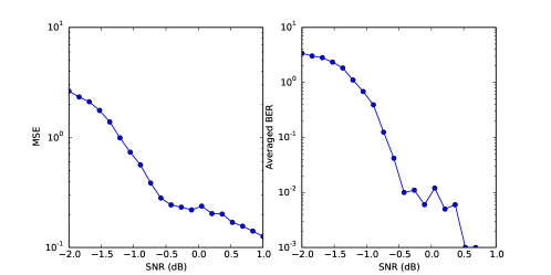
Figure 1: Linear transceiver design.

Numerical result.

In an experiment, $n=10$, $m=15$, $p=10$, and the channel matrix $C$ is a random matrix with IID normal distribution. The signal to noise ratio varies, and for each value of $\sigma_{\mathrm{e}}$, we try to solve the problem to get a design of $A$ and $B$. Each design is tested by $1000$ trials with random signal $x$ and noise $e$ generated from the same distributions as the ones in the design. The method is run without proximal operator and with initial point generated from the SVD of the channel matrix $C$. The mean squared error and the averaged bit error rate are in Figure 1.

6.4 Sparse dictionary learning

Problem description.

The aim is to find a dictionary $D\in{\mbox{\bf R}}^{m\times n}$ under which the data matrix $X\in{\mbox{\bf R}}^{m\times T}$ can be approximated by sparse coefficients, i.e., $X\approx DY$ where $Y\in{\mbox{\bf R}}^{n\times T}$ is a sparse matrix [mairal2009online].

The optimization problem can be formulated as

$$\begin{array}[]{ll}\mbox{minimize}&\frac{1}{2}\|DY-X\|_{F}^{2}+\alpha\|Y\|_{1}\\ \mbox{subject to}&\|D\|_{F}\leq 1,\end{array}$$

where the variables are $Y$ and $D$, and $\alpha>0$ is a parameter. The problem is biconvex.

DMCP specification.

The code can be written as follows.

ΨD = Variable(m,n)
ΨY = Variable(n,T)
Ψalpha = Parameter(sign = ’Positive’)
Ψcost = square(norm(D*Y-X,’fro’))/2+alpha*norm(Y,1)
Ψprob = Problem(Minimize(cost), [norm(D,’fro’) <= 1])
Ψprob.solve(method = ’bcd’)
Ψ

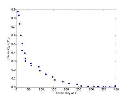
Figure 2: Sparse dictionary learning.

Numerical result.

In an experiment, $X$ is a random normal matrix with $m=10$, $n=20$, and $T=20$. The parameter $\alpha$ is swept from $10^{-5}$ to $1$. For each value of $\alpha$, the method is called with random initialization, and the relative approximation error and the cardinality of $Y$ are shown as a blue dot in Figure 2.

6.5 Sparse feedback matrix design

Problem description.

To design a sparse linear constant output feedback control $u=Ky$ for the system

$$\dot{x}=Ax+Bu,\quad y=Cx,$$

which results in a decay rate $r$ no less than a given threshold $\theta>0$ in the closed-loop system, we consider the following optimization problem [hassibi1999path, boyd1994linear]

$$\begin{array}[]{ll}\mbox{minimize}&\sum_{ij}|K_{ij}|\\ \mbox{subject to}&P\succeq I,\quad r\geq\theta\\ &-2rP\succeq(A+BKC)^{T}P+P(A+BKC),\end{array}$$

where $K$, $P$, and $r$ are variables, and $A$, $B$, $C$, and $\theta$ are given. The notation $P\succeq I$ means that $P-I$ is semidefinite. The problem is biconvex with minimal sets of variables to fix $\{P\}$ and $\{K,r\}$.

DMCP specification.

The code can be the following.

ΨP = Variable(n,n)
ΨK = Variable(m1,m2)
Ψr = Variable(1)
Ψcost = norm(K,1)
Ψconstr = [np.eye(n) << P, r >= theta]
Ψconstr += [(A+B*K*C).T*P+P*(A+B*K*C) << -P*r*2]
Ψprob = Problem(Minimize(cost), constr)
Ψprob.solve(method = ’bcd’)
Ψ

Numerical result.

An example with $n=m_{1}=5$, $m_{2}=4$, $\theta=0.01$, and the following data matrices from [hassibi1999path] is tested.

$$A =\begin{bmatrix}-2.45&-0.90&1.53&-1.26&1.76\\ -0.12&-0.44&-0.01&0.69&0.90\\ 2.07&-1.20&-1.14&2.04&-0.76\\ -0.59&0.07&2.91&-4.63&-1.15\\ -0.74&-0.23&-1.19&-0.06&-2.52\end{bmatrix}$$

$$B =\begin{bmatrix}0.81&-0.79&0&0&-0.95\\ -0.34&-0.50&0.06&0.22&0.92\\ -1.32&1.55&-1.22&-0.77&-1.14\\ -2.11&0.32&0&-0.83&0.59\\ 0.31&-0.19&-1.09&0&0\end{bmatrix}$$

$$C =\begin{bmatrix}0&0&0.16&0&-1.78\\ 1.23&-0.38&0.75&-0.38&0\\ 0.46&0&-0.05&0&0\\ 0&-0.12&0.23&-0.12&1.14\\ \end{bmatrix}$$

The initial value $P^{0}$ is an identity matrix, $r^{0}=1$, and $K^{0}$ is an matrix with all zeros. The result is that $r=0.01$ and

$$K=\begin{bmatrix}0&0.32&0&0\\ 0&-0.46&0&0\\ 0&0&0&0\\ 0&0&0&0\\ 0&0.11&0&0\\ \end{bmatrix},$$

which is sparse. The three nonzero entries are in the second column, so only the second output needs to be fed back. In the work [hassibi1999path] with decay rate no less than $0.35$ another sparse feedback matrix is found with the same cardinality $3$.

6.6 Bilinear control

Problem description.

A discrete time $m$-input bilinear control system is of the following form [hours2014parametric]

$$x_{t+1}=Ax_{t}+\sum_{i=1}^{m}u^{i}_{t}B^{i}x_{t},\quad t=1,\ldots,n-1,$$

where $u_{t}=[u^{1}_{t},\ldots,u^{m}_{t}]\in\Omega\subseteq{\mbox{\bf R}}^{m}$ is the input, and $x_{t}\in{\mbox{\bf R}}^{d}$ is the system state at time $t$. In an optimal control problem with fixed initial state, given system matrices $A,B^{i}\in{\mbox{\bf R}}^{n\times n}$ and convex objective functions $f$ and $g$, an optimization problem can be formulated as

$$\begin{array}[]{ll}\mbox{minimize}&f(x)+g(u)\\ \mbox{subject to}&x_{1}=x_{\mathrm{ini}}\\ &(x_{t},u_{t})\in\Omega,\quad t=1,\ldots,n-1\\ &x_{t+1}=Ax_{t}+\sum_{i=1}^{m}u^{i}_{t}B^{i}x_{t},\quad t=1,\ldots,n-1,\end{array}$$

where $x_{t}$ and $u_{t}$ are variables, and $\Omega$ is a given convex set describing bounds on $u_{t}$ and $x_{t}$. The problem is multi-convex.

As a special case, a standard model of D.C.-motor is a bilinear system of the following form [Derese1982]

$$\dot{x}=A_{0}x+uA_{1}x+bv,$$

where the derivative is with respect to time, and

$$x=\begin{bmatrix}x^{1}\\ x^{2}\end{bmatrix},\quad A_{0}=\begin{bmatrix}-1&0\\ 0&-0.1\end{bmatrix},\quad A_{1}=\begin{bmatrix}0&-19\\ 0.1&0\end{bmatrix},\quad b=\begin{bmatrix}20\\ 0\end{bmatrix}.$$

The correspondence between model and physical variables is that, $x^{1}$ is the armature current, $x^{2}$ is the speed of rotation, $u$ is the field current, and $v$ is the armature voltage. For nominal operation,

$$x^{1}=x^{2}=u=v=1.$$

A control problem is the braking with short-circuited armature ($v_{t}=0$). The field current $u$ is controlled such that the rotation speed decreases to zero as fast as possible, and that the armature current is not excessively large. By discretizing over time and taking $10$ samples per second, the problem can be formulated in the following form

$$\begin{array}[]{ll}\mbox{minimize}&\|x^{2}\|_{2}\\ \mbox{subject to}&x_{1}=\begin{bmatrix}1\\ 1\end{bmatrix}\\ &\max_{t=1,\ldots,n}|x^{1}_{t}|\leq M\\ &(x_{t+1}-x_{t})/0.1=A_{0}x_{t}+u_{t}A_{1}x_{t},\quad t=1,\ldots,n-1,\end{array}$$

where $u\in{\mbox{\bf R}}^{n-1}$ and $x_{t}=[x^{1}_{t},x^{2}_{t}]\in{\mbox{\bf R}}^{2}$ for $t=1,\ldots,n$ are variables, and the notation $x^{i}=[x^{i}_{1},\ldots,x^{i}_{n}]$, $i=1,2$. The problem is biconvex if we consider $x=[x_{1},\ldots,x_{n}]\in{\mbox{\bf R}}^{2\times n}$ as one variable.

DMCP specification.

The code is as the following.

x = Variable(2,n)
u = Variable(n-1)
constr = [x[:,0] == 1, max_entries(abs(x[0,:])) <= M]
for t in range(n-1):
    constr += [x[:,t+1]-x[:,t] == 0.1*(A0*x[:,t]+A1*x[:,t]*u[t])]
prob = Problem(Minimize(norm(x[1,:])), constr)
prob.solve(method = ’bcd’)

Numerical result.

We take an example with $n=100$ and $M=8$. The initial value of $x$ is zero and of $u$ is a vector linearly decreasing from $0.5$ to $0$. The result is shown in Fig. 3, where the braking is faster than that in a linear control system shown in [Derese1982].

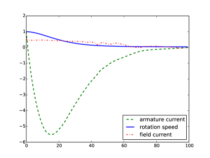
Figure 3: D.C.-motor braking.

6.7 Resistance estimation

Problem description.

A problem in direct current (DC) circuit is to estimate the values of resistors such that certain constraints on currents and voltages can be satisfied. The topology of the circuit is given, and several observations on currents and voltages are known. A general problem of estimating the resistance to fit the topology and the observations can be written as the following

$$\begin{array}[]{ll}\mbox{minimize}&f(u)+g(i)\\ \mbox{subject to}&A(r)i=u\\ &u\in\mathcal{U},\quad i\in\mathcal{I},\quad r\in\mathcal{R},\end{array}$$

where $u\in{\mbox{\bf R}}^{n}$, $i\in{\mbox{\bf R}}^{m}$, and $r\in{\mbox{\bf R}}_{+}^{d}$ are variables representing voltages, currents, and resistance, respectively. The convex functions $f$ and $g$ penalize deviations from the observations. The first constraint corresponds to the Ohm’s law, where the mapping $A$ is linear and depends on the topology of the circuit. The sets $\mathcal{U}$, $\mathcal{I}$, and $\mathcal{R}$ are convex, and they may describe the Kirchhoff’s circuit laws. The problem is multi-convex due to the first constraint.

A simple example is shown in the following circuit diagram.