Invariant manifolds and the parameterization method in coupled energy harvesting piezoelectric oscillators

Abstract

Energy harvesting systems based on oscillators aim to capture energy from mechanical oscillations and convert it into electrical energy. Widely extended are those based on piezoelectric materials, whose dynamics are Hamiltonian submitted to different sources of dissipation: damping and coupling. These dissipations bring the system to low energy regimes, which is not desired in long term as it diminishes the absorbed energy. To avoid or to minimize such situations, we propose that the coupling of two oscillators could benefit from theory of Arnold diffusion. Such phenomenon studies $O(1)$ energy variations in Hamiltonian systems and hence could be very useful in energy harvesting applications. This article is a first step towards this goal. We consider two piezoelectric beams submitted to a small forcing and coupled through an electric circuit. By considering the coupling, damping and forcing as perturbations, we prove that the unperturbed system possesses a $4$-dimensional Normally Hyperbolic Invariant Manifold with $5$ and $4$-dimensional stable and unstable manifolds, respectively. These are locally unique after the perturbation. By means of the parameterization method, we numerically compute parameterizations of the perturbed manifold, its stable and unstable manifolds and study its inner dynamics. We show evidence of homoclinic connections when the perturbation is switched on.

Keywords: damped oscillators, energy harvesting systems, parameterization method, normally hyperbolic invariant manifolds, homoclinic connections, Arnold diffusion.

1 Introduction

Energy harvesting systems consists of devices able to absorb energy from the environment and, typically, electrically power a load or accumulate electrical energy in accumulators (super capacitors or batteries) for later use. One of the most extended approaches is by means of piezoelectric materials, which, under a mechanical strain, generate an electric charge. Such materials are however mostly observed working in the inverse way in, for example, most cell phones: they generate a vibration when driven by a varying voltage.
Most energy harvesting systems based on piezoelectric materials aim to absorb energy from machine vibrations, pedestrian walks or wind turbulences, and can power loads ranging from tiny sensors through small vibrations to small communities through networks of large piezoelectric “towers” submitted to wind turbulences. One of the most extended configurations consists of a piezoelectric beam or cantilever. Due to the viscous nature of the piezoelectric materials, they behave like damped oscillators which, in absence of a strong enough external forcing, tend to oscillate with small amplitude close to the resting position. In order to benefit higher energy oscillations, a typical approach consists of locating two magnets in inverse position as in Figure 1(b). If the magnets are strong enough with respect to the damping of the beam, in the absence of an external forcing, the resting vertical position (previously an attracting focus) becomes an unstable (saddle) equilibrium and two new attracting foci appear pointing to each of the magnets.

\begin{picture}(1.0,0.4)\put(0.0,0.0){ \begin{@subfigure}\includegraphics[width=173.44534pt]{single_piezo/single_piezo}\@@toccaption{{\lx@tag[ ]{{(a)}}{}}}\@@caption{{\lx@tag[ ]{{\footnotesize(a)}}{\footnotesize}}}\end{@subfigure} } \put(0.51,0.0){ \begin{@subfigure}\includegraphics[width=173.44534pt]{single_piezo3/single_piezo}\@@toccaption{{\lx@tag[ ]{{(b)}}{}}}\@@caption{{\lx@tag[ ]{{\footnotesize(b)}}{\footnotesize}}}\end{@subfigure} } \end{picture}

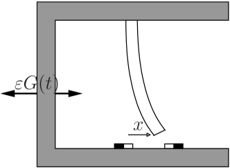
(a)

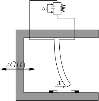
(b)

Figure 1: Generic elastic beam (a) and piezoelectric beam (b) subject to the influence of two magnets and a small periodic forcing.

The equations of motions for a generic (not necessarily piezoelectric) damped and forced beam with magnets as the one shown in Figure 1(a) were first derived in [24], which were shown to be a Duffing equation:

$$\ddot{x}+2\zeta\dot{x}-\frac{1}{2}x\left(1-x^{2}\right)=\varepsilon G(t),$$

where $x$ is the dimensionless horizontal displacement of the lower end, $\zeta$ is the damping coefficient and $\varepsilon G(t)$ a small periodic forcing. When a piezelectric beam is connected to a load in the upper end (as in Figure 1(b)), the load receives a certain power, a voltage $w$, whose time-derivative is proportional to the speed of lower displacement. From the point of view of the load, the piezoelectric beam acts as a capacitor. Hence, the voltage $w$ follows the discharge law of a capacitor:

$$\dot{w}=-\lambda w-\kappa\dot{x},$$

where $\lambda$ is a time constant associated with the capacitance of the piezoelectric beam and the resistance of the load, and $\kappa>0$ is the electrical piezoelectric constant. However, in such a configuration, a mechanical auto-coupling effect occurs: the beam sees its own generated voltage $w$ and the piezoelectric properties of the beam generates a strain opposite to the currently applied one. This not only has a dissipative effect, as it slows down the beam, but also increases the dimension of the system by one (see [10]). The system then becomes:

$$\ddot{x}+2\zeta\dot{x}-\frac{1}{2}x(1-x^{2})-\chi w=\varepsilon G(t)$$

$$\dot{w}=-\lambda w-\kappa\dot{x},$$

where $\chi>0$ is the mechanical piezoelectric constant.

The length of a piezoelectric beams or cantilevers plays a crucial role in the efficiency of the energy harvesting system, as it determines the frequency of the external forcing, $\varepsilon G(t)$, for which the device is “optimal”. Therefore, such devices need to be designed to resonate at a particular frequency. A big effort has been done from the design point of view to broaden this bandwidth. A common approach, introduced in [20], is to consider coupled oscillators of different lengths such that the device exhibits different voltage peaks at different frequencies. Other approaches consider different structural configurations ([12]) to achieve a similar improvement, or study the number of piezoelectric layers connected in different series-parallel configurations ([11]). However, mathematical studies of those models seem relegated to numerical simulations and bifurcation analysis [15, 26, 27]. As it was unveiled in [24], there exist very interesting dynamical phenomena already in the most simple case of a single beam under a periodic forcing (as in Figure 1(a)), such as homoclinic tangles, horseshoes and a Duffing chaotic attractor; also, when neglecting the damping, KAM theorem holds providing the existence of invariant curves. These, in the absence of dissipation, are boundaries in the state space and hence act as energy bounds. Therefore, assuming an external forcing of $O(\varepsilon)$, the amplitude of the oscillations of the beam cannot grow beyond this order hence restricting the amount of energy that can be absorbed from the source.

\begin{picture}(1.0,0.4)\put(0.0,0.0){ \begin{@subfigure}\includegraphics[width=173.44534pt]{coupled_piezo2/coupled_piezo}\@@toccaption{{\lx@tag[ ]{{(a)}}{}}}\@@caption{{\lx@tag[ ]{{\footnotesize(a)}}{\footnotesize}}}\end{@subfigure} } \put(0.51,0.0){ \begin{@subfigure}\includegraphics[width=173.44534pt]{coupled_piezo_spring/coupled_piezo}\@@toccaption{{\lx@tag[ ]{{(b)}}{}}}\@@caption{{\lx@tag[ ]{{\footnotesize(b)}}{\footnotesize}}}\end{@subfigure} } \end{picture}

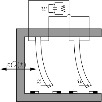
(a)

(b)

Figure 2: (a) Two piezoelectric oscillators coupled through the electrci circuit. (b) Two piezoelectric oscillators with additional conservative coupling (a spring).

Even more interesting from the dynamical point of view is the higher dimensional case when considering two or more coupled damped oscillators. A common approach is to couple them in parallel as in Figure 2(a), although series connection is also used (see [11] for a comparison between parallel and series connection of piezoelectric layers). When connected as in Figure 2(a), the piezoelectric beams become mechanically coupled through the piezoelectric coupling effect: the voltage generated by one beam accelerates or slows down the other one through the electric circuit. This can be modeled with the following equations ([21])

$$\ddot{x}+2\zeta\dot{x}-\frac{1}{2}x(1-x^{2})-\chi w=\varepsilon G(t)$$ (1)

$$\ddot{u}+2\zeta\dot{u}-\frac{1}{2}u(1-u^{2})-\chi w=\varepsilon G(t)$$

$$\dot{w}=-\lambda w-\kappa\left(\dot{x}+\dot{u}\right).$$

Note that the only coupling term, $\chi w$, is dissipative.
When neglecting dissipative terms ($\zeta=\chi=0$), the dimension of KAM tori is not large enough to act as energy bounds and one may observe Arnold diffusion ([1]): existence of trajectories exhibiting $O(1)$ growth in their “energy” when the device is driven by an arbitrarily small periodic forcing ($0<\varepsilon\ll 1$). Therefore, if oscillators are conservatively coupled, the phenomenon of Arnold diffusion could help such devices to exhibit robustness to the frequency of the periodic source and higher efficiency than acting separately. Hence, in order to increase the chances of taking advantage of this phenomenon, we propose to introduce a conservative coupling between the oscillators. Physically, such coupling can be achieved by introducing a spring linking the two beams, as in Figure 2(b). Assuming that beams are equal and that the displacement of their lower ends is only horizontal, the spring is kept horizontal. In this case, the model becomes

$$\ddot{x}+2\zeta\dot{x}-\frac{1}{2}x(1-x^{2})-\chi w-k(u-x)=\varepsilon G(t)$$ (2)

$$\ddot{u}+2\zeta\dot{u}-\frac{1}{2}u(1-u^{2})-\chi w-k(x-u)=\varepsilon G(t)$$

$$\dot{w}=-\lambda w-\kappa\left(\dot{x}+\dot{u}\right),$$

where $k$ is the elastic constant of the spring. These equations are also obtained when linearising around the horizontal position of the beam.

Arnold diffusion was introduced in the celebrated paper of Arnold [1]. Recently, researchers have achieved impressive advances providing rigorous results to prove the existence of such trajectories in general Hamiltonian systems [2, 16, 23]. The most paradigmatic applications of Arnold diffusion are associated with classical problems in celestial mechanics such as instabilities in the restricted three-body problem or the Kirkwood gaps in the asteroids belt of the solar system [13], although it has also been proven in physical examples such as ABC magnetic fields [22]. Partial results have also been proven in mechanical systems with impacts [17].
The main mechanism for diffusion is based on the existence of normally hyperbolic invariant manifolds (NHIMs) containing the mentioned KAM tori. By combining inner dynamics in these manifolds and outer through homoclinic/heteroclinic excursions, such tori can be skipped allowing the trajectories to further accumulate energy from the source. The study of these outer excursions was greatly facilitated by the introduction of the Scattering map [8, 9].

Unfortunately, theory for Arnold diffusion is still too restrictive to be applied in systems of the types (1) and (2), mainly due to the presence of dissipation, as it provides an extra obstacle to the growth of energy.
In this work we present a first step on the study of Arnold diffusion in energy harvesting systems based on damped oscillators. In particular, we focus on a system based on the coupling of two piezoelectric beams as in Figure 2(b) and we perform a theoretical and numerical study of the invariant objects, their dynamics and their connections by means of the parameterization method. These objects play a crucial role in the known mechanisms for Arnold diffusion, given by combination of dynamics close to Normally Hyperbolic Invariant Manifolds (NHIM’s) (inner dynamics) and homoclinic excursions along the intersection of their stable and unstable manifolds. In this article we have a less ambitions goal and we perform a first step in this direction: we perform a theoretical study of the existence and persistence of a NHIM, its numerical computation as well as its inner dynamics and its stable and unstable manifolds by means of the so-called parameterization method [5, 19]. A detailed study of homoclinic intersections and the Scattering map is left for a future work. The main difficulty relies on the dimension of the system, which is $6$-dimensional and the presence of dissipation in both the oscillators (through damping) and the coupling (inverse piezoelectric effect).

This work is organized as follows. In Section 2 we introduce a generalized version of the system in a perturbation setting: forcing, dissipation and coupling are included only in $O(\varepsilon)$ terms. We analyze its invariant objects for the unperturbed case and their persistence after introducing the perturbation. In Section 3 we present the theoretical setting necessary to apply the Newton-like method introduced in [19] based on the parameterization method. In Section 4 we present the obtained numerical results, studying the inner dynamics for different configurations regarding the two types of dissipations (damping and piezoelectric coupling). Finally, we present our conclusions in Section 5.

2 Invariant objects

2.1 Generalization of the model

As mentioned in the introduction, this paper is concerned with the study of invariant manifolds of a particular energy harvesting system consisting of two coupled piezoelectric beams. However, many of the results and techniques that we show are valid for a larger class of systems. Hence, in this section we introduce a general class of systems that for which our results hold. We first consider a Hamiltonian system of the form

$$H_{\varepsilon}(x,y,u,v,s)=\mathcal{X}(x,y)+\mathcal{U}(u,v)+\varepsilon h(x,y,u,v,t),$$ (3)

with $h(x,y,u,v,t+T)=h(x,y,u,v,t)$ and $\varepsilon\geq 0$ a small parameter. Assume that

1. the system associated with the Hamiltonian $\mathcal{X}$ possesses a saddle point, $Q_{0}$, with a homoclinic loop, $\gamma$, parameterized by a function $\sigma(t):\mathbb{R}\to\mathbb{R}^{2}$:

   $$\gamma=\mathcal{W}^{s}(Q_{0})=\mathcal{W}^{u}(Q_{0})=\left\{\sigma(t)\in\mathbb{R}^{2},\,t\in\mathbb{R}\right\}$$

   satisfying

   $$\sigma^{\prime}(t)=\left(\begin{array}[]{cc}0&1\\ -1&0\end{array}\right)\nabla\mathcal{X}(\sigma(t)),$$ (4)

   ($\sigma(t)$ is a solution of the Hamiltonian $\mathcal{X}$) and

   $$\lim_{t\to\pm\infty}\left|\sigma(t)-Q_{0}\right|<\lim_{t\to\pm\infty}Me^{-\tilde{\lambda}\left|t\right|}=0,$$

   for some $M,\tilde{\lambda}>0$,

2. the system associated with the Hamiltonian $\mathcal{U}$ is integrable in some open set in the Liouville sense (can be written in action-angle variables). Moreover, it satisfies the twist condition (associated frequencies of its invariant sets are monotone).

Remark 1.

Alternatively, condition h2 can be stated as follows: “The system associated with Hamiltonian $\mathcal{U}$ possesses a continuum of periodic orbits, $\mathcal{U}(u,v)=c$, whose periods are monotone in $c$”.

Remark 2.

One could assume that $\mathcal{U}(u,v)$ is given in action-angle variables: $U(I,\phi)=\Omega(I)$ with $\Omega^{\prime}(I)\neq 0$. These canonical variables would of course simplify the notation in the theoretical statements. However, in applications, one frequently finds systems that are integrable but are not given in such variables (as it is our case). Provided that this change of variables becomes difficult to explicitly apply, we prefer to keep a general Hamiltonian $U(u,v)$ in order to allow applications to deal with original variables as much as possible.
However, in Section 2.2, it will be useful to introduce a parameterization introducing action-angle-like variables, which can be easily numerically compute.

Remark 3.

Similarly as in Remark 2, the Hamiltonian $X(x,y)$ could be assumed to be a pendulum: $X(x,y)=\frac{y^{2}}{2}+\cos(x)-1$. For the same reason we keep here a general Hamiltonian $X(x,y)$.

To System (3) we add a small dissipative coupling given by an extra equation leading to the $5$-dimensional non-autonomous system

$$\dot{z} =J_{1}\nabla\mathcal{X}(u,v)+J_{2}\nabla\mathcal{U}(x,y)$$ (5)

$$\quad+\varepsilon\Big{(}J_{3}\nabla h(z,t)+\nu g(z,w)\Big{)}$$

$$\dot{w} =-\lambda w+b(z),$$

where $z=(x,y,u,v)$,

$$J_{1}=\left(\begin{array}[]{cc}0&1\\ -1&0\\ 0&0\\ 0&0\end{array}\right),\quad J_{2}=\left(\begin{array}[]{cc}0&0\\ 0&0\\ 0&1\\ -1&0\end{array}\right)$$

and

$$J_{3}=\left(\begin{array}[]{cccc}0&1&0&0\\ -1&0&0&0\\ 0&0&0&1\\ 0&0&-1&0\end{array}\right).$$

While $\varepsilon$ is a perturbative parameter ($0\leq\varepsilon\ll 1$), $\nu$ is not necessary small. The latter allows to couple and uncouple system $z$ with $w$, distinguishing between a conservative and dissipative behaviour regarding coordinates $z$.

By adding time as a variable, $t=s\in\mathbb{T}_{T}=\mathbb{R}/T\mathbb{Z}$, and calling $\tilde{z}=(z,w,s)\in\mathbb{R}^{5}\times\mathbb{T}_{T}$, we write system (5) in an autonomous and more compact form as

$$\dot{\tilde{z}}=g_{0}(\tilde{z})+\varepsilon\left(g_{1}(\tilde{z})+\nu g_{2}(\tilde{z})\right)$$ (6)

with

$$g_{0}(\tilde{z})=\left(\begin{array}[]{c}J_{1}\nabla\mathcal{X}(x,y)+J_{2}\nabla\mathcal{U}(u,v)\\ -\lambda w+b(z)\\ 1\end{array}\right),$$

$$g_{1}(\tilde{z})=\left(\begin{array}[]{c}g(z,w)\\ 0\\ 0\end{array}\right)$$

and

$$g_{2}(\tilde{z})=\left(\begin{array}[]{c}J_{3}\nabla h(x,y,v,s)\\ 0\\ 0\end{array}\right).$$

Note that $g_{1}$ contains the dissipative terms and coupling while $g_{2}$ the conservative coupling and forcing.

2.2 Invariant objects of the unpertubed system

For $\varepsilon=0$, the unperturbed system (6) becomes

$$\dot{\tilde{z}}=g_{0}(\tilde{z}),$$ (7)

which consists of the crossed product of systems $(x,y)$, $(u,v)$, $w$ and $s$.
As system $\mathcal{U}$ is integrable, it possesses periodic orbits given by

$$\mathcal{P}^{c}=\left\{(u,v)\in\mathbb{R}^{2},\,|\,\mathcal{U}(u,v)=c\right\},$$ (8)

whose period, $T_{c}$, is monotone with $c$ due to the twist condition. Assume $T^{\prime}_{c}>0$.
In order to construct a Normally Hyperbolic Invariant Manifold for system (7), we focus on these periodic orbits for system $\mathcal{U}$ while system $\mathcal{X}$ remains at the hyperbolic point $Q_{0}=(0,0)$. Provided that each of these periodic orbits is contained in the energy level given by $\mathcal{U}(u,v)=c$, as mentioned in Remark 2, it will be useful to parametrize them by $c$ and an angle, $\theta$. Hence we will consider “action angle”-like variables $(\theta,c)\in\mathbb{T}\times\mathbb{R}$ to parametrize periodic orbits $\mathcal{P}^{c}$ as follows. Let $\varphi_{\mathcal{U}}(t;u_{0},v_{0})$ be the flow associated with system $\mathcal{U}$, such that $\varphi_{\mathcal{U}}(0;u_{0},v_{0})=(u_{0},v_{0})$. Choose a section in $\mathbb{R}^{2}$ transversal to all periodic orbits $\mathcal{U}(u,v)=c$, and let $(u_{c},v_{c})$ the point in that section at level of energy $c$. Then we consider the parameterization

$$\begin{array}[]{cccc}p:&\mathbb{T}\times\mathbb{R}&\longrightarrow&\mathbb{R}^{2}\\ &(\theta,c)&\longmapsto&\varphi_{\mathcal{U}}(\theta T_{c};u_{c},v_{c}).\end{array}$$ (9)

As for action-angle variables, this change of variables can be difficult (or impossible) to apply explicitly. However, as we will show in Sections 3.2 and 4, it can be easily numerically implemented.

The following lemma gives as the existence of a Normally Hyperbolic Invariant Manifold for System (6) when $\varepsilon=0$.

Lemma 1.

1. System (7) possesses a foliated $3$-dimensional invariant manifold

   $$\tilde{\mathcal{K}}=Q_{0}\times\bigcup_{c_{1}\leq c\leq c_{2}}\tilde{\mathcal{K}}^{c}$$

   with

   $$\tilde{\mathcal{K}}^{c}= \Big{\{}(u,v,w,s)\in\mathcal{P}^{c}\times\mathbb{R}\times\mathbb{T}_{T},\,|\,w=w^{p}_{0}(u,v)\Big{\}}$$

   $$\mathcal{P}^{c} =\Big{\{}(u,v)\in\mathbb{R}^{2},\,|\,\mathcal{U}(u,v)=c\Big{\}}$$

   $$w^{p}_{0}(u,v) =\frac{e^{-\lambda T_{c}}}{1-e^{-\lambda T_{c}}}\int_{0}^{T_{c}}b(Q_{0},\varphi_{\mathcal{U}}(s;u,v))ds$$ (10)

   These objects can be written by means of the parameterizations

   $$\begin{array}[]{cccc}p:&\mathbb{T}\times(0,\infty)&\longrightarrow&\mathbb{R}^{2}\\ &(\theta,c)&\longmapsto&\varphi_{\mathcal{U}}(\theta T_{c};u_{c},v_{c})\end{array}$$

   $$\begin{array}[]{cccc}\tilde{K}^{c}:&\mathbb{T}\times\mathbb{T}_{T}&\longrightarrow&\mathbb{R}^{3}\times\mathbb{T}_{T}\\ &(\theta,s)&\longmapsto&\left(p(\theta,c),w^{p}_{0}(p(\theta,c)),s\right)\end{array}$$

   $$\begin{array}[]{cccc}\tilde{K}:&\mathbb{T}\times\mathbb{R}\times\mathbb{T}_{T}&\longrightarrow&\mathbb{R}^{5}\times\mathbb{T}_{T}\\ &(\theta,c,s)&\longmapsto&\left(Q_{0},\tilde{K}^{c}(\theta,s)\right)\end{array}$$

   such that

   $$\mathcal{P}^{c} =p(\mathbb{T},c)$$

   $$\tilde{\mathcal{K}}^{c} =\tilde{K}^{c}(\mathbb{T},\mathbb{T}_{T})$$

   $$\tilde{\mathcal{K}} =\tilde{K}(\mathbb{T},[c_{1},c_{2}],\mathbb{T}_{T}).$$

2. The manifold $\tilde{\mathcal{K}}$ is normally hyperbolic, has a $5$-dimensional stable manifold

   $$\mathcal{W}^{s}(\tilde{\mathcal{K}})=\mathcal{W}^{s}(Q_{0})\times\bigcup_{c\in[c_{1},c_{2}]}\mathcal{P}^{c}\times\mathbb{R}\times\mathbb{T}_{T}$$

   and a $4$-dimensional unstable manifold forming a homoclinic manifold,

   $$\tilde{\Gamma}=\mathcal{W}^{u}(\tilde{\mathcal{K}})\subset\mathcal{W}^{s}(\tilde{\mathcal{K}}),$$

   where

   $$\tilde{\Gamma} =\bigcup_{c_{1}\leq c\leq c_{2}}\Big{\{}\left(\sigma(\tau),u,v,w,s\right)\in\mathcal{P}^{c}\times\gamma\times\mathbb{R}\times\mathbb{T}_{T},$$

   $$\qquad\tau\in\mathbb{R},\,w=w^{u}_{0}(\tau,u,v)\Big{\}}$$

   and

   $$w^{u}_{0}(\tau,u,v) =\int_{-\infty}^{0}\Big{(}b\big{(}\sigma(\tau+s),\varphi_{\mathcal{U}}(s;u,v)\big{)}-b\big{(}Q_{0},\varphi_{\mathcal{U}}(s;u,v)\big{)}\Big{)}e^{\lambda s}ds$$

   $$+w^{p}_{0}(u,v).$$

   The unstable and stable manifolds can be parameterized by

   $$\mathcal{W}^{s}(\tilde{\mathcal{K}}) =\tilde{W}^{s}(\mathbb{T},[c_{1},c_{2}],\mathbb{T}_{T},\mathbb{R}^{2})$$

   $$\mathcal{W}^{u}(\tilde{\mathcal{K}}) =\tilde{W}^{u}(\mathbb{T},[c_{1},c_{2}],\mathbb{T}_{T},\mathbb{R}),$$

   where

   $$\begin{array}[]{cccc}\tilde{W}^{s}:&\mathbb{T}\times[c_{1},c_{2}]\times\mathbb{T}_{T}\times\mathbb{R}^{2}&\longrightarrow&\mathbb{R}^{5}\times\mathbb{T}_{T}\\ &(\theta,c,s,\tau,r)&\longmapsto&\left(\sigma(\tau),p(\theta,c),r,s\right)\end{array}$$

   $$\begin{array}[]{cccc}\tilde{W}^{u}:&\mathbb{T}\times[c_{1},c_{2}]\times\mathbb{T}_{T}\times\mathbb{R}&\longrightarrow&\mathbb{R}^{5}\times\mathbb{T}_{T}\\ &(\theta,c,s,\tau)&\longmapsto&\left(\sigma(\tau),p(\theta,c),w^{u}_{0}(\tau,p(\theta,c)),s\right)\end{array}$$

Proof.

When $(x,y)=Q_{0}$, provided that $\lambda>0$, the variable $w$ is attracted to a certain object given by the dynamics of $v$. Given $(u_{0},v_{0})$ we define

$$b^{p}(t;u_{0},v_{0})=b\left(Q_{0},\varphi_{\mathcal{U}}(t;u_{0},v_{0})\right).$$ (11)

Then the dynamics of $w$ restricted to $(x,y)=Q_{0}$ is given by

$$\dot{w}=-\lambda w+b^{p}(t;u_{0},v_{0}).$$ (12)

Provided that Equation (12) is linear in $w$ and $b^{p}(t;u_{0},v_{0})$ is $T_{c}$-periodic, System (12) possesses an $T_{c}$-periodic orbit:

$$w^{p}(t+T_{c})=w^{p}(t),$$

which is attracting (because $\lambda>0$).
We compute the initial condition for such periodic orbit. Note that, although system (12) is not autonomous, we can assume that the intial conditions are given for $t=0$, since Equation (12) has to be integrated together with the equations for $\dot{u}$ and $\dot{v}$, which provides a $3$-dimensional autonomous system. Therefore, the general solution of (12) becomes

$$w(t;w_{0},u_{0},v_{0})=e^{-\lambda t}\left(\int_{0}^{t}b^{p}(s;u_{0},v_{0})e^{\lambda s}ds+w_{0}\right),$$

from where, imposing $w(T_{c};w_{0})=w_{0}$, we get that the initial condition for a periodic orbit is

$$w^{p}_{0}(u_{0},v_{0})=\frac{e^{-\lambda T_{c}}}{1-e^{-\lambda T_{c}}}\int_{0}^{T_{c}}b^{p}(s;u_{0},v_{0})e^{\lambda s}ds.$$

Hence, given $(u_{0},v_{0})$, the attracting periodic orbit of $w$ becomes

$$w^{p}(t) =e^{-\lambda t}\Bigg{(}\int_{0}^{t}b^{p}(s;u_{0},v_{0})e^{\lambda s}ds$$ (13)

$$\quad+\frac{e^{-\lambda T_{c}}}{1-e^{-\lambda T_{c}}}\int_{0}^{T_{c}}b^{p}(s;u_{0},v_{0})e^{\lambda s}ds\Bigg{)}.$$

Note that $w^{p}_{0}$ depends on $u_{0}$ and $v_{0}$ through the periodic orbit (11). Moreover, $w_{0}^{p}(u_{0},v_{0})$ is indeed a parametrization of the whole periodic orbit $w^{p}(t)$: just by keeping $t=0$ and varying $u_{0},v_{0}$ along the periodic orbit $\mathcal{P}^{c}$ $w_{0}^{p}(u_{0},v_{0})$ evolves along the periodic orbit $w^{p}(t)$. Hence we have obtained the $3$-dimensional invariant manifold

$$\tilde{\mathcal{K}}=Q_{0}\times\left(\bigcup_{c_{1}\leq c\leq c_{2}}\Big{\{}\left(u,v,w\right)\,|\,\,\mathcal{U}(u,v)=c,\,w=w^{p}_{0}(u,v)\Big{\}}\right)\times\mathbb{T}_{T}\subset\mathbb{R}^{5}\times\mathbb{T}_{T}.$$

Recalling that $(u_{0},v_{0})$ can be parametrized by $p(\theta,c)$ as in Equation (9), $w_{0}^{p}$ can be as well parametrized by $\theta$ and $c$: $w_{0}^{p}=w_{0}^{p}(p(\theta,c))$. This induces a parametrization for $\tilde{\mathcal{K}}$

$$\tilde{K}:\mathbb{T}\times\mathbb{R}\times\mathbb{T}_{T}\longrightarrow\mathbb{R}^{5}\times\mathbb{T}_{T},$$

given by

$$\tilde{K}(\theta,c,s)=\left(\begin{array}[]{c}0\\ 0\\ p(\theta,c)\\ w^{p}_{0}(p(\theta,c))\\ s\end{array}\right)$$

and hence

$$\tilde{\mathcal{K}}=\tilde{K}(\mathbb{T},[c_{1},c_{2}],\mathbb{T}_{T}).$$

The invariant manifold $\tilde{\mathcal{K}}$ is foliated by $2$-dimensional invariant tori contained at the energy level $c$:

$$\tilde{\mathcal{K}}=Q_{0}\times\bigcup_{c_{1}\leq c\leq c_{2}}\tilde{\mathcal{K}}^{c}.$$

Each of these tori is homeomorphic to $\mathbb{T}\times\mathbb{T}_{T}$,

$$\tilde{\mathcal{K}}^{c}\simeq\mathbb{T}\times\mathbb{T}_{T},$$

as it can be parametrized by $(\theta,s)$:

$$\tilde{\mathcal{K}}^{c}=\tilde{K}^{c}\left(\mathbb{T},c,\mathbb{T}_{T}\right),$$

where

$$\tilde{K}^{c}:\mathbb{T}\times\mathbb{T}_{T}\longrightarrow\mathbb{R}^{3}\times\mathbb{T}_{T}$$

and

$$\tilde{K}^{c}(\theta,s) =\Pi_{u,v,w,s}\left(\tilde{K}(\theta,c,s)\right)$$

$$=(p(\theta,c),w_{0}^{p}(p(\theta,c)),s).$$

We now show that the invariant manifold $\tilde{\mathcal{K}}$ is normally hyperbolic by showing that it has stable/unstable normal bundles with exponential convergence/divergence.
By fixing coordinates $(\theta,c,s)$, we focus on a point at the manifold $\tilde{\mathcal{K}}$,

$$K(\theta,c,s)=\tilde{z}^{b}=(Q_{0},u,v,w_{0}^{p}(u,v)),s)\in\tilde{\mathcal{K}},$$ (14)

and we study its stable and unstable fibers.

Clearly, hyperbolicity is inherited from the hyperbolic point $Q_{0}$. Hence, coordinates $(x,y)$ of points of the invariant fibers of $\tilde{z}^{b}$ are given by the homoclinic loop of $Q_{0}$, parametrized by $\tau$:

$$\sigma(\tau)\in\gamma.$$ (15)

Coordinates $(u,v,s)$ need to be equal those of $\tilde{z}^{b}$ due to their lack of hyperbolicity. So it only remains to find proper values of $w$ to define the stable and unstable fibers of $\tilde{z}^{b}$.

Letting $\varphi_{\mathcal{X}}(t;x,y)$ be the flow associated with the Hamiltonian $\mathcal{X}$ we define

$$b^{h}(t;\tau,u,v) =b\Big{(}\varphi_{\mathcal{X}}\big{(}t;\sigma(\tau)\big{)},\varphi_{\mathcal{U}}\big{(}t;u,v\big{)}\Big{)}$$

$$=b(\sigma(\tau+t),\varphi(t;u,v)).$$

The last equality holds due to condition given in Equation (4).
For $(x,y)\in\gamma$, the variable $w$ evolves following the equation

$$\dot{w}=-\lambda w+b^{h}(t;\tau,u,v),$$

which has the general solution

$$w(t;w_{0})=e^{-\lambda t}\left(w_{0}+\int_{0}^{t}b^{h}\left(s;\tau,u,v)\right)e^{\lambda s}ds\right).$$ (16)

Then, the values $w_{0}^{s}$ and $w_{0}^{u}$ that we are looking need to satisfy

$$\lim_{t\to\infty}\left|w(t;w^{s}_{0})-w(t;w_{0}^{p})\right|\longrightarrow 0$$

and

$$\lim_{t\to-\infty}\left|w(t;w^{u}_{0})-w(t;w_{0}^{p})\right|\longrightarrow 0.$$

We define

$$z(t;z_{0})=w(t;w_{0})-w(t;w_{0}^{p}),$$

with

$$z_{0}=w_{0}-w^{p}_{0}.$$

Defining

$$b^{z}(t;\tau,u,v)=b^{h}(t;\tau,u,v)-b^{p}(t;u,v),$$

$z(t)$ becomes

$$z(t)=e^{-\lambda t}\left(z_{0}+\int_{0}^{t}b^{z}(s;\tau,u,v)e^{\lambda s}ds\right).$$

Due to the hyperbolicity of $Q_{0}$ and the fact that $b(x,y,u,v)$ is continuous, we know that there exist positive constants $\tilde{\lambda}$, $M$ and $\delta$ such that

$$\left|b^{z}(t;\tau,u,v)\right|<Me^{-\tilde{\lambda}\left|t\right|}$$

if $\left|t\right|>\delta$.
On one hand, we get that

$$\lim_{t\to+\infty}\left|z(t)\right| =\lim_{t\to+\infty}\left|e^{-\lambda t}z_{0}+\int_{0}^{t}b^{z}(s;\tau,u,v)e^{\lambda(s-t)}ds\right|$$

$$<\lim_{t\to+\infty}M\int_{0}^{t}e^{-\tilde{\lambda}s+\lambda(s-t)}ds=0,$$

for any $z_{0}\in\mathbb{R}$. As a consequence, all initial conditions $w_{0}$ are attracted to the periodic orbit $w^{p}(t)$. Hence, the stable fiber leaves $w$ free.
On the other hand, the limit for $t\to-\infty$ diverges unless we choose

$$z_{0}(\tau,u,v)=\int_{-\infty}^{0}b^{z}(s;\tau,u,v)e^{\lambda s}ds.$$

In this case, we get

$$\lim_{t\to-\infty}\left|z(t)\right| =\lim_{t\to-\infty}\left|e^{-\lambda t}\Bigg{(}\int_{-\infty}^{0}e^{\lambda s}b^{z}(s)ds+\int_{0}^{t}e^{\lambda s}b^{z}(s)ds\Bigg{)}\right|$$

$$=\lim_{t\to-\infty}\left|e^{-\lambda t}\int_{-\infty}^{t}e^{\lambda s}b^{z}(s)ds\right|$$

$$<\lim_{t\to-\infty}\left|e^{-\lambda t}\int_{-\infty}^{t}Me^{(\lambda+\tilde{\lambda})s}ds\right|$$

$$=\lim_{t\to-\infty}\frac{Me^{\tilde{\lambda}t}}{\lambda+\tilde{\lambda}}=0.$$

Therefore, the unstable fiber of $\tilde{z}^{b}$ is given by points $(\sigma(\tau),u,v,w_{0}^{u},s)$ with

$$w_{0}^{u}(\tau,u,v) =\int_{-\infty}^{0}b^{h}(s;\tau,u,s)e^{\lambda s}ds+w_{0}^{p}(u,v)$$

$$=\int_{-\infty}^{0}\Big{(}b\big{(}\sigma(\tau+s),\varphi_{\mathcal{U}}(s;u,v)\big{)}$$

$$\qquad-b(Q_{0},\varphi_{\mathcal{U}}(s;u,v))\Big{)}e^{\lambda s}ds+w_{0}^{p}(u,v).$$

∎

Remark 4.

When $c$ is such that $T$ and $T_{c}$ are congruent, then $\tilde{\mathcal{K}}^{c}$ is filled by periodic orbits: each point is a periodic point of the $T$-time return map. However, when $T$ and $T_{c}$ are inconmensurable, $\tilde{\mathcal{K}}^{c}$ is densily filled by the trajecteory of any point at $\tilde{\mathcal{K}}^{c}$. Note that this implies that, for any initial condition at the invariant manifold $\tilde{\mathcal{K}}$, one obtains bounded dynamics both for $t\to\infty$ and $t\to-\infty$.

Remark 5.

The manifolds $\mathcal{W}^{s}(\tilde{\mathcal{K}})$ and $\mathcal{W}^{u}(\tilde{\mathcal{K}})$ generate the normal bundle to $\tilde{\mathcal{K}}$, as they generate the $x-y$ plane and the stable manifold contains the hyperplane $w$.

2.3 Persistence of manifolds

In order to study the persistence of the manifold $\tilde{\mathcal{K}}$ for $\varepsilon>0$, we use theory for normally hyperbolic invariant manifolds ([14]). However, due to the presence of dissipation for $\nu>0$, the resulting manifold may lose some properties. This is summarized in the following

Proposition 1.

For $\varepsilon>0$ and some $c_{0}>0$, there exists a unique parameterization

$$\tilde{K}_{\varepsilon}:\mathbb{T}\times[c_{1},c_{2}]\times\mathbb{T}_{T}\longrightarrow\mathbb{R}^{5}\times\mathbb{T}_{T}$$

with $0<c_{0}<c_{1}<c_{2}$, such that, the manifold $\tilde{\mathcal{K}}_{\varepsilon}=\tilde{K}_{\varepsilon}(\mathbb{T},[c_{1},c_{2}],\mathbb{T}_{T})$ is unique, normally hyperbolic and $\varepsilon$-close to $\tilde{K}_{0}=\tilde{K}$. Moreover,

1. if $\nu=0$, $\tilde{\mathcal{K}}_{\varepsilon}$ is invariant and has boundaries,

2. if $\nu>0$, the manifold $\tilde{K}_{\varepsilon}(\mathbb{T},(c_{1},c_{2}),\mathbb{T}_{T})$ is locally invariant.

Proof.

For $\varepsilon>0$ theory of normally hyperbolic invariant manifolds ([14]) guarantees that (locally) there exists $\tilde{\mathcal{K}}_{\varepsilon}$ $\varepsilon$-close to $\tilde{\mathcal{K}}$, with $\tilde{\mathcal{K}}_{0}=\tilde{\mathcal{K}}$.
If $\nu=0$, the perturbation in System (6) becomes Hamiltonian and, hence, the dynamics of the system restricted to $\tilde{\mathcal{K}}_{\varepsilon}$ (inner dynamics) becomes symplectic. In this case, KAM theory ([7]) provides the existence of invariant tori in $\tilde{\mathcal{K}}_{\varepsilon}$ bounding the inner dynamics. Assuming $c_{1}$ and $c_{2}$ are chosen such that $T_{c_{1}}/T$ and $T_{c_{2}}/T$ are diophantine, the manifold $\tilde{\mathcal{K}}_{\varepsilon}$ has boundaries given by the invariant tori $\tilde{K}_{\varepsilon}(\mathbb{T},c_{1},\mathbb{T}_{T})$ and $\tilde{K}_{\varepsilon}(\mathbb{T},c_{2},\mathbb{T}_{T})$. As a consequence, the manifold is invariant.

When the perturbation includes dissipative terms ($\nu>0$), the existence of these boundaries is not guaranteed, as KAM tori are generically destroyed ([6]). Therefore, in this case, $\tilde{\mathcal{K}}_{\varepsilon}$ does not necessary possess boundaries. However, we show that it is unique. We consider $[c_{1}^{\prime},c_{2}^{\prime}]$ such that $c_{1}^{\prime}>0$ and $[c_{1},c_{2}]\subset[c_{1}^{\prime},c_{2}^{\prime}]$, and construct a new smooth field $g^{\prime}_{\varepsilon}(\tilde{z})$ coinciding with (6) for $c\in(c_{1}^{\prime},c_{2}^{\prime})$ and vanishing otherwise. This guarantees the existence of a “larger” normally hyperbolic invariant manifold, $\tilde{\mathcal{K}}_{\varepsilon}^{\prime}$, $\varepsilon$-close to $\tilde{K}_{0}(\mathbb{T},[c_{1}^{\prime},c_{2}^{\prime}],\mathbb{T}_{T})$ and possessing boundaries. Therefore, theory for normally hyperbolic invariant manifolds holds and $\tilde{\mathcal{K}}_{\varepsilon}^{\prime}$ is unique and invariant. As $\tilde{\mathcal{K}}_{\varepsilon}\subset\tilde{\mathcal{K}}_{\varepsilon}^{\prime}$ and $g_{\varepsilon}^{\prime}$ coincides with $g_{0}+\varepsilon(g_{1}+\nu g_{2})$ in $\tilde{\mathcal{K}}_{\varepsilon}$, the manifold $\tilde{\mathcal{K}}_{\varepsilon}$ is also unique.
Although, due to the dissipation, inner dynamics contains attractors, trajectories may leave $\tilde{\mathcal{K}}_{\varepsilon}$ both when flown forwards or backwards in time. This however occurs slowly and points away from original boundaries $c=c_{1}$ and $c=c_{2}$ remain in $\tilde{\mathcal{K}}_{\varepsilon}$ for large periods of time. Therefore, the manifold $\tilde{K}_{\varepsilon}(\mathbb{T},(c_{1},c_{2}),\mathbb{T}_{T})$ becomes only locally invariant.

∎

Remark 6.

These parameterizations, together with the dynamics of the system restricted to $\tilde{\mathcal{K}}_{\varepsilon}$ and linear approximations of the manifolds $\mathcal{W}_{\varepsilon}^{s}(\tilde{\mathcal{K}}_{\varepsilon})$ and $\mathcal{W}_{\varepsilon}^{u}(\tilde{\mathcal{K}}_{\varepsilon})$ will be numerically computed in Section 3 by means of the parameterizaiton method.

Remark 7.

The constant $c_{0}$ guarantees that $c_{1}$ is enough isolated from $c=0$. If this does not occur, then the manifold $\tilde{\mathcal{K}}_{\varepsilon}$ may lose normal hyperbolicity, as the tangent dynamics start competing with the normal ones when periodic orbits $\mathcal{P}^{c}$ are too close to the homoclinic loop. However, this loss of normal hyperbolicity can be avoided by considering beams of different lengths leading to different hyperbolic rates.

Remark 8.

From Proposition 1 we also get parameterizations for the stable and unstable manifolds of $\tilde{\mathcal{K}}_{\varepsilon}$:

$$\tilde{W}^{s,\pm}_{\varepsilon} :\mathbb{T}\times[c_{1},c_{2}]\times\mathbb{T}_{T}\times\mathbb{R}^{2}\longrightarrow\mathbb{R}^{5}\times\mathbb{T}_{T}$$ (17)

$$\tilde{W}^{u,\pm}_{\varepsilon} :\mathbb{T}\times[c_{1},c_{2}]\times\mathbb{T}_{T}\times\mathbb{R}\longrightarrow\mathbb{R}^{5}\times\mathbb{T}_{T}$$ (18)

2.4 Two-coupled piezoelectric oscillators

In this section we apply the previous results to the case of two coupled piezo-electric oscillators. We first write System (2) as in Equation (6).
Let us assume that the damping ($\zeta$), the piezolectric coupling ($\chi$) and the elastic constant of the spring ($k$) are small. We introduce scalings to write these parameters in terms of the amplitude of the small forcing as follows

$$\zeta=\varepsilon\tilde{\zeta},\quad\chi=\varepsilon\tilde{\chi},\quad k=\varepsilon\tilde{k}.$$ (19)

The parameter $\nu$ in Equation (19) is not a real parameter of the system but it is artificially introduced in order to allow distinguishing between a conservative case ($\nu=0$) and the general dissipative one ($\nu>0$) so. This situation can be distinguished between $\tilde{\zeta}=\tilde{\chi}=0$ or $\tilde{\zeta}>0$ and/or $\tilde{\chi}>0$. Therefore, when dealing with the real model of coupled piezo-electric oscillators we will ignore $\nu$.
The scalings (19) allow us to write System (2) in the perturbative form given in Equations (3)-(5) with

$$\mathcal{X}(x,y) =\frac{y^{2}}{2}-\frac{1}{4}x^{2}\left(1-\frac{x^{2}}{2}\right)$$ (20)

$$\mathcal{U}(u,v) =\frac{v^{2}}{2}-\frac{1}{4}u^{2}\left(1-\frac{u^{2}}{2}\right)$$ (21)

$$h(z,t) =-\frac{\tilde{k}}{2}(u-x)^{2}-(x+u)G(t)$$ (22)

$$g(z) =\tilde{\chi}w$$ (23)

$$b(z) =-\kappa(y+v).$$ (24)

Note that System (2) has been reduced to a first order system be adding the variables $y=\dot{x}$ and $v=\dot{u}$.
In the autonomous and more compact form given in Equation (6), the functions $g_{i}$ become

$$g_{0}(\tilde{z})=\left(\begin{array}[]{c}y\\ \frac{1}{2}x(1-x^{2})\\ v\\ \frac{1}{2}u(1-u^{2})\\ -\lambda w-\kappa(y+v)\\ 1\end{array}\right)$$ (25)

$$g_{1}(\tilde{z})=\left(\begin{array}[]{c}0\\ -2\tilde{\zeta}y+\tilde{\chi}w\\ 0\\ -2\tilde{\zeta}v+\tilde{\chi}w\\ 0\\ 0\end{array}\right)$$ (26)

and

$$g_{2}(\tilde{z})=\left(\begin{array}[]{c}0\\ k(u-x)+G(s)\\ 0\\ k(x-u)+G(s)\\ 0\\ 0\end{array}\right).$$ (27)

For $\varepsilon=0$, the $(x,y,u,v)$ system becomes two uncoupled and unforced beams modeled by the Hamiltonians $\mathcal{X}$ and $\mathcal{U}$. In this case, these Hamiltonians are equal, but satisfy conditions  h1–h2. The phase portrait for each Hamiltonian is shown in Figure 3 and consists of a figure of eight.

Figure 3: Phase portrait of each beam in absence of forcing, damping and coupling.

It possesses three equilibrium points, two of the elliptic type, $Q^{\pm}=(\pm 1,0)$, and a saddle point at the origin, $Q_{0}=(0,0)$. The latter possesses two homoclinic loops, $\gamma^{\pm}$, each surrounding the elliptic points $Q^{\pm}$, and located at the level $\left\{\mathcal{X}(x,y)=0\right\}$:

$$\gamma^{+}\cup\left\{Q_{0}\right\}\cup\gamma^{-}=\left\{(x,y)\in\mathbb{R}^{2},\,\mathcal{X}(x,y)=0\right\}.$$

Therefore, the Hamiltonian $\mathcal{X}$ satisfies condition h1 where the homoclinic loop $\gamma$ can be either $\gamma^{+}$ or $\gamma^{-}$, which are parameterized by two different parameterizations $\sigma^{\pm}$ satisfying

$$\gamma^{\pm}=\left\{\sigma^{\pm}(t),\,t\in\mathbb{R}\right\}$$ (28)

$$\lim_{t\to\pm\infty}\sigma^{\pm}(t)=Q_{0}$$

$$\sigma^{\pm}(0)=(0,\pm\sqrt{2}).$$

Regarding the Hamiltonian $\mathcal{U}$, there exist three regions where it is integrable and satisfies condition h2. Two of these three regions are the ones surrounded by the homoclinic loops $\gamma^{\pm}$ and containing the elliptic points $Q^{\pm}$, and satisfy $\left\{-\frac{1}{8}<U(u,v)<0\right\}$. The third region consists of the outer part to homoclinic loops, given by $\left\{U(u,v)>0\right\}$. These three regions are covered by a continum of periodic orbits with growing period as approaching the homoclinic loop, hence satisfying condition h2.
From the applied point of view, we are interested on having as much energy as possible. Therefore, we will focus on the higher energy periodic orbits located in this third region, as they provide larger amplitude oscillations. Similar invariant objects to the ones we will construct in Section 2.2 can be obtained when focusing on the other two regions surrounding each of the elliptic points $Q^{\pm}$.

For $\varepsilon=0$, the parameterizations given in Lemma 1 become as follows. We first fix the transversal section to the periodic orbits as $u=0$. Hence, we get $(u_{c},v_{c})=(0,\sqrt{2c})$ and the action-angle-like parameterization of the periodic orbits becomes

$$\begin{array}[]{cccc}p:&\mathbb{T}\times\mathbb{R}&\longrightarrow&\mathbb{R}^{2}\\ &(\theta,c)&\longmapsto&\varphi_{\mathcal{U}}(\theta T_{c};0,\sqrt{2c}).\end{array}$$ (29)

Provided the form of the Hamiltonian $\mathcal{U}$, we can obtain expressions for the periods of $\mathcal{P}^{c}$ as follows. The periodic orbit with initial condition $(0,\sqrt{2c})$ crosses the $u$ axis at the point

$$\left(u_{1},0\right)=\left(\sqrt{1+\sqrt{1+8c}},0\right).$$

Using the symmetries of the system and its Hamiltonian structure, we obtain that the period of the periodic orbit $\mathcal{P}^{c}$ becomes

$$T_{c}:= 4\int_{0}^{u_{1}}\frac{1}{\dot{u}}du$$ (30)

$$= 4\int_{0}^{u_{1}}\frac{1}{\sqrt{2c+\frac{u^{2}}{2}\left(1-\frac{u^{2}}{2}\right)}}du.$$

However, as it will be detailed in Section 3.2, when numerically computed, it becomes better to compute $T_{c}$ using a Newton method instead of numerically computing the integral (30).
We also get more concrete expressions for the parameterization of $\tilde{\mathcal{K}}$ given in Lemma 1. In partilar, $w_{0}^{p}$ and $w_{0}^{u}$ become

$$w^{p}_{0}(u,v) =-\frac{e^{-\lambda T_{c}}}{1-e^{-\lambda T_{c}}}\int_{0}^{T_{c}}\kappa v^{p}(s;u,v)e^{\lambda s}ds$$ (31)

$$v^{p}(s;u,v) =\Pi_{v}\left(\varphi_{\mathcal{U}}(s;u,v)\right),$$

and

$$w^{u}_{0}(\tau,u,v) =-\int_{-\infty}^{0}\kappa e^{\lambda s}y^{h}(s;\tau)ds+w^{p}_{0}(u,v)$$ (32)

$$y^{h}(s;\tau) =\Pi_{y}\left(\sigma(\tau+s)\right),$$

where $\sigma$ can be either $\sigma^{+}$ or $\sigma^{-}$.

3 Numerical framework for the parameterization method

In this section we present a method to numerically compute the perturbed Normally Hyperbolic Manifold $\tilde{\mathcal{K}}_{\varepsilon}$ by means of the so-called parameterization method, introduced in [3, 4, 5]. This method is the one presented in [19], Chapter 5.
The parameterization method is stated easier when formulated for maps; hence, it will be more convenient to write the full system (6) as discrete system. The most natural map to consider is of course the stroboscopic map, due to the periodicity of the system. However, due to the foliated nature of the unperturbed manifold $\tilde{\mathcal{K}}_{0}$, instead of using the original variables, we will consider from now on the induced map in the manifolds introduced in Section 2.4:

$$\begin{array}[]{cccc}F_{\varepsilon}:&\mathbb{T}\times(0,\infty)\times\mathbb{R}^{3}&\longrightarrow&\mathbb{T}\times(0,\infty)\times\mathbb{R}^{3}\\ &(\theta,c,x,y,w)&\longmapsto&\tilde{p}\circ\mathfrak{s}_{\varepsilon}\circ\tilde{p}^{-1}(\theta,c,x,y,w),\end{array}$$ (33)

where $\tilde{p}$ is the extended version of the change of variables (29),

$$\tilde{p}(\theta,c,x,y,w)=(x,y,p(\theta,c),w)=(x,y,\varphi_{\mathcal{U}}(\theta T_{c};u_{c},v_{c}),w),$$

and $\mathfrak{s}_{\varepsilon}$ is the stroboscopic map

$$\begin{array}[]{cccc}\mathfrak{s}_{\varepsilon}:&\Sigma_{s}&\longrightarrow&\Sigma_{s+T}\\ &(x,y,u,v,w)&\longmapsto&\tilde{\phi}_{\varepsilon}(s+T;x,y,u,v,w,s),\end{array}$$

being $\tilde{\phi}_{\varepsilon}$ the flow associated with the full system (6).
Arguing as in Section 2.3, by considering the flow $g^{\prime}$ we obtain a map $F^{\prime}_{\varepsilon}$ and a parameterization

$$K_{\varepsilon}:\mathbb{T}\times[c_{1}^{\prime},c_{2}^{\prime}]\longrightarrow\mathbb{T}\times[c_{1}^{\prime},c_{2}^{\prime}]\times\mathbb{R}^{3},$$ (34)

such that the manifold

$$\mathcal{K}^{\prime}_{\varepsilon}=K_{\varepsilon}(\mathbb{T}\times[c_{1}^{\prime},c_{2}^{\prime}])$$

is unique, normally hyperbolic and invariant under $F_{\varepsilon}^{\prime}$. Moreover, $F_{\varepsilon}^{\prime}$ and $F_{\varepsilon}$ coincide in $\mathcal{K}^{\prime}_{\varepsilon}$. By restricting the parameterization $K_{\varepsilon}$ to $[c_{1},c_{2}]$, we obtain a manifold,

$$\mathcal{K}_{\varepsilon}=K_{\varepsilon}(\mathbb{T},[c_{1},c_{2}]),$$

which is unique and normally hyperbolic. Although it is locally invariant, $\mathcal{K}_{\varepsilon}$ contains the image of those points isolated enough from the boundaries of $\mathcal{K}_{0}$ ($c=c_{1}$ and $c=c_{2}$).
The map $F_{\varepsilon}$ restricted to $K_{\varepsilon}$ induces inner dynamics in $\mathcal{K}_{\varepsilon}$ given by a map

$$f_{\varepsilon}:\mathbb{T}\times[c_{1},c_{2}]\longrightarrow\mathbb{T}\times[c_{1}^{\prime},c_{2}^{\prime}].$$

We find the inner dynamics $f_{\varepsilon}$ and the parameterization $K_{\varepsilon}$, using the parameterization, that is, by imposing that the diagram

$$\begin{CD}\mathbb{T}\times[c_{1},c_{2}]@>{K_{\varepsilon}}>{}>\mathbb{T}\times[c_{1},c_{2}]\times\mathbb{R}^{3}\\ @V{}V{f_{\varepsilon}}V@V{}V{F_{\varepsilon}}V\\ \mathbb{T}\times[c_{1}^{\prime},c_{2}^{\prime}]@>{K_{\varepsilon}}>{}>\mathbb{T}\times[c_{1}^{\prime},c_{2}^{\prime}]\times\mathbb{R}^{3}\end{CD}$$

commutes.
Note that, although we do not have an explicit expression for the map $F_{\varepsilon}$, we can consider that it is given provided that we can numerically compute the stroboscopic map $\mathfrak{s}$ just by integrating the system. Hence, we need to solve the cohomological

$$F_{\varepsilon}\circ K_{\varepsilon}-K_{\varepsilon}\circ f_{\varepsilon}=0$$ (35)

for the unknowns $f_{\varepsilon}$ and $K_{\varepsilon}$. We do this by following the method described in [19] (Chapter 5). It consists of taken advantage of the hyperbolicity of $\mathcal{K}_{\varepsilon}$ to perform a Newton-like method to compute functions $f_{\varepsilon}$ and $K_{\varepsilon}$. In practice, given a discretization of the reference manifold $\mathbb{T}_{T}\times[c_{1},c_{2}]$, this means that we want to compute the coefficients for approximations (splines, Fourier series or Lagrangian polynomials) of $f_{\varepsilon}$ and $K_{\varepsilon}$. We first review the method described in [19] adapted to our case.

3.1 A Newton-like method

Assume that, for a certain $\varepsilon>0$, we have good enough approximations of $K_{\varepsilon}$ and $f_{\varepsilon}$. As usual in Newton-like methods, in order to provide improved approximations, we will require as well an initial guess of the dynamics at the tangent bundles; that is, approximations of the solutions to the cohomological equation

$$DF_{\varepsilon}\left(K_{\varepsilon}\left(\theta,c\right)\right)-DK_{\varepsilon}(f_{\varepsilon}(\theta,c))=0.$$ (36)

Note that Equation (36) manifests the invariance of the tangent bundle $T\mathcal{K}_{\varepsilon}$ under $DF_{\varepsilon}$, leading to inner dynamics at $T\mathcal{K}_{\varepsilon}$ given by $Df_{\varepsilon}$. However, $DF_{\varepsilon}$ is a map onto the tangent space $T\left(\mathbb{T}\times\mathbb{R}\times\mathbb{R}^{3}\right)$. The latter can be generated by two vectors in $T\mathcal{K}_{\varepsilon}$ and three in the normal bundle $N\mathcal{K}_{\varepsilon}$, $T\left(\mathbb{T}\times\mathbb{R}\times\mathbb{R}^{3}\right)=T\mathcal{K}_{\varepsilon}\times N\mathcal{K}_{\varepsilon}$. Provided that $\mathcal{K}_{\varepsilon}$ is normally hyperbolic, the normal space $N\mathcal{K}_{\varepsilon}$ can be generated by two vectors tangent to $\mathcal{W}^{s}(\mathcal{K}_{\varepsilon})$ and a third one tangent to $\mathcal{W}^{u}(\mathcal{K}_{ề})$. It will be hence useful to consider the adapted frame around $\mathcal{K}_{\varepsilon}$

$$P_{\varepsilon}(\theta,c)=\left(L_{\varepsilon}(\theta,c)\,N_{\varepsilon}(\theta,c)\right),$$

given by the juxtaposition of the matrices $L_{\varepsilon}$ and $N_{\varepsilon}$, where

$$L_{\varepsilon}(\theta,c)=DK_{\varepsilon}(\theta,c)$$

is a $5\times 2$ matrix and $N_{\varepsilon}(\theta,c)$ is $5\times 3$ given by the three columns of $DF_{\varepsilon}$ generating the normal bundle $N\mathcal{K}_{\varepsilon}$.
The matrix $P_{\varepsilon}$ can be seen as a change of basis such that the skew product

$$(f_{\varepsilon},\Lambda_{\varepsilon}):\mathbb{T}\times[c_{1},c_{2}]\times\mathbb{R}^{5}\longrightarrow\mathbb{T}\times[c_{1},c_{2}]\times\mathbb{R}^{5},$$

with

$$\Lambda_{\varepsilon}=P_{\varepsilon}(f(\theta,c))^{-1}DF_{\varepsilon}(K_{\varepsilon}(\theta,c))P_{\varepsilon}(\theta,c),$$

becomes of the form

$$\Lambda_{\varepsilon}=\left(\begin{array}[]{ccccc}\lx@intercol\hfil\hbox{\multirowsetup$\Lambda^{L}_{\varepsilon}$}\hfil\lx@intercol&0&0&0\\ &&0&0&0\\ 0&0&\lx@intercol\hfil\hbox{\multirowsetup$\Lambda^{S}_{\varepsilon}$}\hfil\lx@intercol&0\\ 0&0&&&0\\ 0&0&0&0&\Lambda^{U}_{\varepsilon}\end{array}\right).$$

Note that

$$\Lambda^{L}_{\varepsilon}=Df_{\varepsilon}.$$

The Newton-like method consists of two steps. Given approximations of $K_{\varepsilon}$ (and hence $L_{\varepsilon}=DK_{\varepsilon}$), $f_{\varepsilon}$ (and hence $\Lambda^{L}_{\varepsilon}=Df_{\varepsilon}$), $\Lambda^{S}_{\varepsilon}$ and $\Lambda^{N}_{\varepsilon}$, in the first step, one computes new corrected versions of $K_{\varepsilon}$ and $f_{\varepsilon}$ (and hence corrected versions of $L_{\varepsilon}$ and $\Lambda^{L}_{\varepsilon}$). In the second step, one corrects the normal bundle $N_{\varepsilon}$ and its linearized dynamics $\Lambda^{N}_{\varepsilon}$.

3.1.1 First step: correction of the manifold and the inner dynamics

As in [19], we consider corrections of the form

$$\bar{f}_{\varepsilon} =f_{\varepsilon}+\Delta f_{\varepsilon}$$

$$\bar{K}_{\varepsilon} =K_{\varepsilon}+\Delta K_{\varepsilon},$$

with

$$\Delta K_{\varepsilon}=P_{\varepsilon}(\theta,c)\zeta(\theta,c).$$

We want to compute $\zeta(\theta,c)$ and $\Delta f_{\varepsilon}(\theta,c)$.
The corrections of the manifold, $\zeta(\theta,c)$, can be split in tangent, stable and unstable directions:

$$\zeta(\theta,c)=\left(\begin{array}[]{c}\zeta^{L}(\theta,c)\\ \zeta^{S}(\theta,c)\\ \zeta^{U}(\theta,c)\end{array}\right)\in\mathbb{R}^{2}\times\mathbb{R}^{2}\times\mathbb{R}.$$

Let $E(\theta,c)$ be the error at Equation (35) at the current value $f_{\varepsilon}$ and $K_{\varepsilon}$,

$$E(\theta,c)=F_{\varepsilon}(K_{\varepsilon}(\theta,c))-K_{\varepsilon}(f_{\varepsilon}(\theta,c)).$$

Let

$$\eta(\theta,c)=-\left(P(f(\theta,c))\right)^{-1}E(\theta,c),$$

which, again, we split in tangent, stable and unstable directions

$$\eta(\theta,c)=\left(\begin{array}[]{c}\eta^{L}(\theta,c)\\ \eta^{S}(\theta,c)\\ \eta^{U}(\theta,c)\end{array}\right).$$

Then, assuming that

$$\zeta^{L}(\theta,c)=\left(\begin{array}[]{c}0\\ 0\end{array}\right),$$

that is, the manifold $K_{\varepsilon}(\mathbb{T},[c_{1},c_{2}])$ is only corrected in the normal directions, $\Delta f_{\varepsilon}$ becomes

$$\Delta f_{\varepsilon}(\theta,c)=-\eta^{L}(\theta,c)$$

(see [19] for more details).
Regarding $\Delta K_{\varepsilon}$, by expanding Equation (35), one gets that $\zeta^{S}$ and $\zeta^{U}$ satisfy the equations

$$\eta^{S}(\theta,c) =\Lambda^{S}_{\varepsilon}(\theta,c)\zeta^{S}(\theta,c)-\zeta^{S}(\theta,c)$$ (37)

$$\eta^{U}(\theta,c) =\Lambda^{U}_{\varepsilon}(\theta,c)\zeta^{U}(\theta,c)-\zeta^{U}(\theta,c).$$ (38)

Due to hyperbolicity, $\Lambda^{U}_{\varepsilon}>1$ and the eigenvalues of $\Lambda^{S}_{\varepsilon}$ are real, positive and inside the unite circle. Hence, Equations (37)-(38) can be solved by iterating the systems

$$\zeta^{S}(\theta,c) =\Lambda^{S}_{\varepsilon}(f^{-1}(\theta,c))\zeta^{S}(f^{-1}(\theta,c))-\eta^{S}(f^{-1}(\theta,c))$$

$$\zeta^{U}(\theta,c) =\frac{\zeta^{U}(f(\theta,c))+\eta^{U}(\theta,c)}{\Lambda^{U}_{\varepsilon}(\theta,c)}.$$

3.1.2 Second step: normal bundle correction

Once we have new corrected versions of the inner dynamics $f_{\varepsilon}(\theta,c)$ (and consequently $\Lambda^{L}_{\varepsilon}(\theta,c)$) and the parametrization $K_{\varepsilon}(\theta,c)$ (and consequently $L_{\varepsilon}(\theta,c)$), the second step consists of computing new approximations for $\Lambda^{S}_{\varepsilon}$, $\Lambda^{U}_{\varepsilon}$ and $N_{\varepsilon}(\theta,c)$. As in [19], we consider approximations of the form

$$\bar{N}_{\varepsilon}(\theta,c) =N_{\varepsilon}(\theta,c)+\Delta N(\theta,c)$$

$$\bar{\Lambda}^{S}_{\varepsilon}(\theta,c) =\Lambda^{S}_{\varepsilon}(\theta,c)+\Delta\Lambda^{S}(\theta,c)$$

$$\bar{\Lambda}^{U}_{\varepsilon}(\theta,c) =\Lambda^{U}_{\varepsilon}(\theta,c)+\Delta\Lambda^{U}(\theta,c),$$

with

$$\Delta N(\theta,c)=P_{\varepsilon}(\theta,c)Q^{N}(\theta,c).$$

Assuming that the corrections of the linearised stable and unstable bundles are applied only in the complementary directions, one gets that $Q^{N}(\theta,c)$ is of the form

$$Q^{N}(\theta,c)=\left(\begin{array}[]{ccc}\lx@intercol\hfil\hbox{\multirowsetup$Q^{LS}(\theta,c)$}\hfil\lx@intercol&\hbox{\multirowsetup$Q^{LU}(\theta,c)$}\\ &&\\ 0&0&\hbox{\multirowsetup$Q^{SU}(\theta,c)$}\\ 0&0&\\ \lx@intercol\hfil Q^{US}(\theta,c)\hfil\lx@intercol&0\end{array}\right).$$

Let us write the current error in the cohomological equation at the tangent bundle (Equation (36)) as

$$E_{\text{red}}^{N}(\theta,c) =P_{\varepsilon}(\theta,c)^{-1}DF_{\varepsilon}\left(K_{\varepsilon}(\theta,c)\right)N_{\varepsilon}(\theta,c)-$$

$$-\left(\begin{array}[]{ccc}0&0&0\\ 0&0&0\\ \lx@intercol\hfil\hbox{\multirowsetup$\Lambda_{\varepsilon}^{S}(\theta,c)$}\hfil\lx@intercol&0\\ &&0\\ 0&0&\Lambda^{U}_{\varepsilon}(\theta,c)\end{array}\right)=\left(\begin{array}[]{ccc}\lx@intercol\hfil\hbox{\multirowsetup$E_{\text{red}}^{LS}(\theta,c)$}\hfil\lx@intercol&\hbox{\multirowsetup$E_{\text{red}}^{LU}(\theta,c)$}\\ &&\\ \lx@intercol\hfil\hbox{\multirowsetup$E_{\text{red}}^{SS}(\theta,c)$}\hfil\lx@intercol&\hbox{\multirowsetup$E_{\text{red}}^{SU}(\theta,c)$}\\ &&\\ \lx@intercol\hfil E_{\text{red}}^{US}(\theta,c)\hfil\lx@intercol&E_{\text{red}}^{UU}(\theta,c)\end{array}\right)$$

On one hand, the corrections of the adapted frame in the normal directions become

$$\Delta\Lambda^{S}(\theta,c) =E_{\text{red}}^{SS}(\theta,c)$$

$$\Delta\Lambda^{U}(\theta,c) =E_{\text{red}}^{UU}(\theta,c).$$

On the other hand, the corrections of normal part of the change of basis $P_{\varepsilon}(\theta,c)$, are obtained by iterating the systems

$$Q^{LS}(\theta,c) =\left(\Lambda^{L}_{\varepsilon}(\theta,c)\right)\left(Q^{LS}(f(\theta,c))\Lambda^{S}_{\varepsilon}(\theta,c)-E_{\text{red}}^{LS}(\theta,c)\right)$$

$$Q^{LU}(\theta,c) =\frac{\Lambda_{\varepsilon}^{L}(f^{-1}(\theta,c))+E_{\text{red}}^{LU}(f^{-1}(\theta,c))}{\Lambda^{U}_{\varepsilon}(f^{-1}(\theta,c))}$$

$$Q^{US}(\theta,c) =\frac{Q^{US}(f(\theta,c))\Lambda^{S}_{\varepsilon}(\theta,c)-E_{\text{red}}^{US}(\theta,c)}{\Lambda^{U}_{\varepsilon}(\theta,c)}$$

$$Q^{SU}(\theta,c) =\frac{\Lambda^{S}_{\varepsilon}(f^{-1}(\theta,c))Q^{SU}(f^{-1}(\theta,c))+E_{\text{red}}^{SU}(f^{-1}(\theta,c))}{\Lambda^{U}_{\varepsilon}(f^{-1}(\theta,c))}.$$

3.2 Computation of bundles, maps and frames for the unperturbed piezoelectric system

We now derive semi-explicit expressions for the objects for $\varepsilon=0$ for system (6) with $g_{i}$ given in Equations (25)-(27): $f_{0}(\theta,c)$, $F_{0}(\theta,c,x,y,w)$,$DF_{0}(\theta,c)$ and $P_{0}(\theta,c)$. The expressions below have to be partially solved numerically. By semi-explicit we mean that we will assume that computations such us numerical integration or differentiation is exact.

For $\varepsilon=0$, the map $F_{0}(\theta,c,x,y,w)$ consists of computing the stroboscopic map, integrating system (7), from $t_{0}$ to $t_{0}+T$. However, we first need to compute the change of variables $p(\theta,c)=(u,v)$, which requires the computation of $T_{c}$. The expression in Equation (30) implies computing an improper integral provided that $\dot{u}=0$ at $u=u_{1}$, which is numerically problematic. Instead, we perform a Newton method to find the smallest $t^{*}>0$ such that

$$\Pi_{u}\left(\varphi_{\mathcal{U}}(t^{*};0,\sqrt{2c})\right)=0.$$

Then $T_{c}=2t^{*}$ due to the symmetry of the system. This is given by iterating the system

$$t_{i+1}=t_{i}-\frac{\Pi_{u}\left(\varphi_{\mathcal{U}}(t_{i};0,\sqrt{2c})\right)}{\Pi_{v}\left(\varphi_{\mathcal{U}}(t_{i};0,\sqrt{2c})\right)},$$

which allows to obtain a very accurate solution (precision around $10^{-12}$ using order $7--8th$ order Runge Kutta integrator) in few iterations assuming that a good enough first guess is provided.
For $\varepsilon=0$, the system is autonomous and the stroboscopic map does not depend on $t_{0}$; it becomes

$$\mathfrak{s}_{0}(x,y,p(\theta,c),w)=\left(\begin{array}[]{c}\varphi_{\mathcal{X}}(T;x,y)\\ \varphi_{\mathcal{U}}(\theta T_{c}+T;0,\sqrt{2c})\\ w(T;w)\end{array}\right),$$

where $w(t;w)$ is the solution of equation

$$\dot{w}=-\lambda w-k(\Pi_{y}\left(\varphi_{\mathcal{X}}(t;x,y)\right)+\Pi_{v}(\varphi_{\mathcal{U}}(\tau;p(\theta,c)))).$$ (39)

Recall that, as mentioned in Section 2.4, Equation (39) can be seen as a one-dimensional non-autonomous differential equation, assuming that the flows $\varphi_{\mathcal{X}}$ and $\varphi_{\mathcal{U}}$ are known, but indeed depends on the initial values $x,y,u,v$.
Writing $\mathfrak{s}_{0}$ in variables $\theta,c$, we obtain the map $F_{0}$

$$F_{0}(\theta,c,x,y,w)=\left(\begin{array}[]{c}\theta+\frac{T}{T_{c}}\\ c\\ \varphi_{\mathcal{X}}(T;x,y)\\ w(T;w)\end{array}\right),$$

and we assume that we can integrate system $\mathcal{X}$ and Equation (39) “exactly”.
For $\varepsilon=0$ the parameterization $K_{0}(\theta,c)$ becomes

$$K_{0}(\theta,c)=\left(\begin{array}[]{c}\theta\\ c\\ 0\\ 0\\ w^{p}_{0}(p(\theta,c))\end{array}\right).$$

Again, we need to compute $w^{p}_{0}(p(\theta,c))$ numerically. One option is to numerically perform the integral given in Equation (10). However, it becomes faster an more precise to compute $w^{p}_{0}(p(\theta,c))$ as the solution of a fixed point equation. Recall that, when restricted to the manifold $\tilde{K}_{0}$, $(x,y)$ are kept constant to $(0,0)$, and hence the dynamics is given by system $\mathcal{U}$ and $\dot{w}$ as given in Equation (11), which we recall here for commodity

$$\left.\begin{aligned} \dot{u}&=v\\ \dot{v}&=\frac{1}{2}u\left(1-u^{2}\right)\\ \dot{w}&=\lambda w-kv\end{aligned}\right\}.$$ (40)

Let $\varphi_{\mathcal{U}w}(t;u,v,w)$ be the flow associated with system (40). Then, $w^{p}_{0}(p(\theta,c))$ is the solution for $w_{0}$ of the fixed point equation

$$\Pi_{w}\left(\varphi_{\mathcal{U}w}(T_{c};p(\theta,c),w_{0})\right)-w_{0}=0,$$ (41)

which we can solve using a Newton method. Provided that $T_{c}$ does not depend on $w_{0}$, the derivative $\partial_{w_{0}}\Pi_{w}\left(\varphi_{\mathcal{U}x}(\alpha;p(\theta,c),w_{0})\right)$, necessary for the Newton method, can be obtained by integrating the variational equations of system (40) from $t=0$ to $t=T_{c}$.

We next get

$$L_{0}(\theta,c)=DK_{0}(\theta,c)=\left(\begin{array}[]{cc}1&0\\ 0&1\\ 0&0\\ 0&0\\ \frac{\partial w^{p}_{0}(\theta,c)}{\partial\theta}&\frac{\partial w_{0}^{p}(\theta,c)}{\partial c}\end{array}\right),$$

and we need to numerically compute the last row. Assuming that we have obtained $w^{p}_{0}(p(\theta,c))$, this can be done by applying the implicit function theorem to Equation (41), which leads to

$$\frac{\partial w^{p}_{0}(p(\theta,c))}{\partial\theta} =-\frac{\overbrace{D_{uv}\Pi_{w}\left(\varphi_{\mathcal{U}w}(T_{c};u,v,w_{0}^{p}(u,v))\right)_{(u,v)=p(\theta,c)}}^{*}\cdot D_{\theta}p(\theta,c)}{\underbrace{\partial_{w_{0}}\Pi_{w}\left(\varphi_{\mathcal{U}w}(T_{c};p(\theta,c),w_{0})\right)_{w_{0}=w_{0}^{p}(\theta,c)}}_{*}-1}$$

$$\frac{\partial w^{p}_{0}(p(\theta,c))}{\partial c} =-\frac{\overbrace{\Pi_{w}\left(\varphi_{\mathcal{U}w}^{\prime}(T_{c};p(\theta,c),w^{p}_{0}(p(\theta,c)))\right)}^{-\lambda w^{p}_{0}(p(\theta,c))-k\Pi_{v}(p(\theta,c))}\cdot\alpha^{\prime}(c)}{\partial_{w_{0}}\Pi_{w}\left(\varphi_{\mathcal{U}w}\left(T_{c};p(\theta,c),w_{0}\right)\right)_{w_{0}=w_{0}^{p}(\theta,c)}-1}-$$

$$\quad-\frac{\overbrace{D_{uv}\varphi_{\mathcal{U}w}(T_{c};u,v,w^{p}_{0}(p(\theta,c)))_{(u,v)=p(\theta,c)}}^{*}\cdot D_{c}p(\theta,c)}{\underbrace{\partial_{w_{0}}\Pi_{w}\left(\varphi_{\mathcal{U}w}\left(T_{c};p(\theta,c),w_{0}\right)\right)_{w_{0}=w_{0}^{p}(\theta,c)}}_{*}-1}.$$

The terms labeled with $*$ can be obtained by integrating the variational equations of system (40), so we still need to obtain $\alpha^{\prime}(c)$ and $D_{\theta c}p(\theta,c)$. The former one is computed by finite differences provided that we can accurately compute $\alpha_{c+h}$ and $\alpha_{c-h}$ for a small enough $h>0$. The latter becomes

$$Dp(\theta,c) =D_{\theta,c}\varphi_{\mathcal{U}}(\theta T_{c};0,\sqrt{2c})$$

$$=D_{uv}\varphi_{\mathcal{U}}(\theta T_{c};u,v)_{(u,v)=p(\theta,c)}\cdot\left(\begin{array}[]{cc}0&0\\ 0&\frac{1}{\sqrt{2c}}\end{array}\right),$$

where $D_{uv}\varphi_{\mathcal{U}}(\theta T_{c};u,v)$ can be obtained integrating the variational equations associated with system $\mathcal{U}$.

We now compute

$$DF_{0}(\theta,c,x,y,w)=\left(\begin{array}[]{ccccc}-\frac{T}{T_{c}^{2}}\alpha^{\prime}(c)&1&0&0&0\\ 0&1&0&0&0\\ 0&0&\lx@intercol\hfil\hbox{\multirowsetup$D_{xy}\varphi_{\mathcal{X}}(T;x,y)$}\hfil\lx@intercol&0\\ 0&0&&&0\\ \partial_{\theta}w^{\prime}&\partial_{c}w^{\prime}&\partial_{x}w^{\prime}&\partial_{y}w^{\prime}&\partial_{w}w^{\prime}\end{array}\right),$$

where $w^{\prime}=w(2\pi/\omega;w)$ is the solution of Equation (39) which, as emphasized above, depends also on $\theta,c,x,y$. The first element of $DF_{0}$ requires computing $\alpha^{\prime}(c)$, which we have already seen. The rest of the elements of $DF_{0}$ can be computed by integrating the full unperturbed system (7) together wit its variational equations.

When evaluated at the manifold $\mathcal{K}_{0}$, the eigenvectors of $DF_{0}$ provide proper directions to split the normal space in stable and unstable directions and hence to obtain the matrix $N_{0}(\theta,c)$.
As shown in Lemma (1), at each point of the manifold $\tilde{K}_{0}$ (similarly for $\mathcal{K}_{0}$) the normal bundle is split in two stable directions and an unstable one. One stable direction is given by the contraction in $w$; the other two are given by the stable and unstable directions of the saddle point $Q_{0}$ of system $\mathcal{X}$. These directions are given by the eigenvectors of matrix $DF_{0}(\tilde{K}_{0})$

$$v_{1}^{s} =\left(0,0,1,-1/\sqrt{2},P_{5,3}\right)$$

$$v_{2}^{s} =\left(0,0,0,0,1\right)$$

$$v^{u} =\left(0,0,1,1/\sqrt{2},P_{5,5}\right),$$

with

$$P_{5,3} =\frac{1/\sqrt{2}\partial_{y}w^{\prime}-\partial_{x}w^{\prime}}{\partial_{w}w^{\prime}+1/\sqrt{2}}$$

$$P_{5,5} =-\frac{1/\sqrt{2}\partial_{y}w^{\prime}+\partial_{x}w^{\prime}}{\partial_{w}w^{\prime}-1\sqrt{2}}.$$

Hence, $N_{0}(\theta,c)$ becomes

$$N_{0}(\theta,c)=\left(\begin{array}[]{ccc}0&0&0\\ 0&0&0\\ 1&0&1\\ -1/\sqrt{2}&0&1/\sqrt{2}\\ P_{5,3}&1&P_{5,5}\end{array}\right).$$

4 Numerical results

We apply the method described in [19] (summarized in Sections 3.1-3.2) to the map given in Equation (33) and corresponding to the stroboscopic map of System (6) with $\mathcal{X}$, $\mathcal{U}$, $h$, $g$ and $b$ given in Equations (20)–(24). We hence will obtain numerical computations of the discrete versions of the Normally Hyperbolic Manifold $\tilde{\mathcal{K}}_{\varepsilon}$ and its associated invariant manifolds $\mathcal{W}^{s}(\tilde{\mathcal{K}}_{\varepsilon})$ and $\mathcal{W}^{u}(\tilde{\mathcal{K}}_{\varepsilon})$. We fix the following parameter values

$$G(t) =\sin(\omega t) \omega =2.1$$

$$\lambda =0.02 \tilde{k}=\kappa =1$$

and consider different situations regarding parameters $\varepsilon$, $\tilde{\zeta}$ and $\tilde{\chi}$. For each of them, we use as seed for the Newton method the unperturbed setting shown in Section 3.2 and use cubic spline interpolations in a grid of points for $(\theta,c)\in\mathbb{T}\times[0.1,1.4]$. At each Newton step, the two substeps explained in Sections 3.1.1 and 3.1.2 are performed for each point of the grid, which allows a natural parallelization. This is done using OpenMP libraries and, ran in a 8 cores node with multithreading (16 threads), each Newton step takes around 2 minutes for a grid of $500\times 200$ points. The code is available at

https://github.com/a-granados/nhim_parameterization

4.1 Conservative case

We start by setting $\tilde{\zeta}=\tilde{\chi}=0$ and $\varepsilon=6\cdot 10^{-2}$. In this case, only the conservative terms of the coupling between the oscillators remain active, as $\tilde{k}=1$. The inner dynamics, restricted to $\tilde{\mathcal{K}}_{\varepsilon}$, is given by the one and a half degrees of freedom Hamiltonian system

$$\mathcal{U}(u,v)+\varepsilon h\left(\Pi_{x,y,u,v,s}\left(\tilde{K}_{\varepsilon}\left(p^{-1}_{\varepsilon}(u,v),s\right)\right)\right),$$

and therefore $f_{\varepsilon}$ becomes a symplectic map.

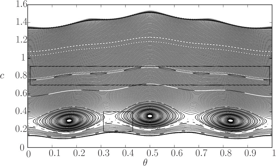
Figure 4: Inner dynamics in $\mathcal{K}_{\varepsilon}$ for the conservative case with $\varepsilon=6\cdot 10^{-2}$ and $\tilde{\zeta}=\tilde{\chi}=0$, obtained by iterating the numerically obtained map $f_{\varepsilon}(\theta,c)$. The labeled rectangles are magnified in Figures 7 and 8.

In Figure 4 we show the global picture of the inner dynamics, where one can see typical objects of this type of maps. The space is mostly covered by KAM invariant curves acting as energy bounds. For the chosen value of $\omega$ one observes three main resonances: $3:1$, $5:2$ and $7:3$, where $m:n$ means $mT=nT_{c}$.

Figure 5: Periods of the unperturbed system, $T_{c}$.

These resonances are labeled in Figure 5, where we show the periods ($T_{c}$) of the unperturbed system as a function of $c$, and they approximately correspond to the unperturbed periodic orbits $\mathcal{P}_{0.325}$, $\mathcal{P}_{0.638}$ and $\mathcal{P}_{0.81}$ defined in Equation (8), respectively. As it comes from Melnikov theory (see [18]) for subharmonics orbits, when they persist, one finds an even number of periodic orbits of the stroboscopic map; half are of the saddle and the rest are elliptic; this number is given by the number of simple zeros of the so-called Melnikov function for subharmonic periodic orbits. Recalling that we are dealing with the conservative case ($\varepsilon>0$, $\tilde{\zeta}=\tilde{\chi}=0$), in our case this function becomes

$$M(t_{0})=\int_{0}^{mT}v(t)\left(\tilde{k}u(t)+G(t+t_{0})\right)dt,$$ (42)

where $(u(t),v(t))=\varphi_{\mathcal{U}}(t;0,\sqrt{2c})$ is evaluated along the unperturbed periodic orbit, $\mathcal{P}^{c}$, with initial condition at $u=0$ and satisfying $T_{c}=mT/n$.

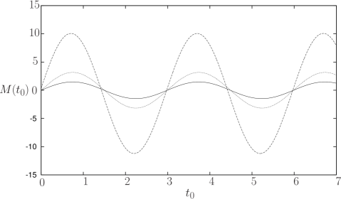
Figure 6: Melnikov functions for the resonances $3:1$ (solid), $7:3$ (dashed, magnified by a factor of $10^{2}$) and $5:2$ (pointed, magnified by a factor of $10^{5}$).

In Figure 6 we show such function for these three resonances. Each of them possesses two simple zeros and, hence, there exist (for $\varepsilon>0$ small enough) two periodic points of the stroboscopic map of the saddle and elliptic type. By adding higher harmonics to $G(t)$, function $M(t_{0})$ may possess more simple zeros. Note that all shown three functions have simple zeros at $t_{0}=0$, which, recalling that the initial condition to compute $M(t_{0})$ is taken at $u=0$, implies that the corresponding periodic orbits possess one point $\varepsilon$-close to $\theta=0$. Note also that the $7:3$ and $5:2$ Melnikov functions have been magnified by a factor $100$ and $10000$, respectively, which tells us which of them will first bifurcate when increasing $\varepsilon$.
The $3:1$ periodic orbits are clearly observed in Figure 4.

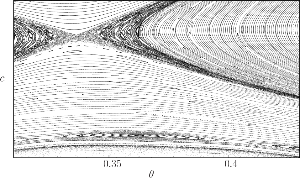
Figure 7: Blow up of the $3:1$ resonance labeled in Figure 4

The saddle type one is magnified in Figure 7, where one also observes secondary tori and evidence of chaos given by the homoclinic tangles. The resonance $7:3$ is magnified in Figure 8.

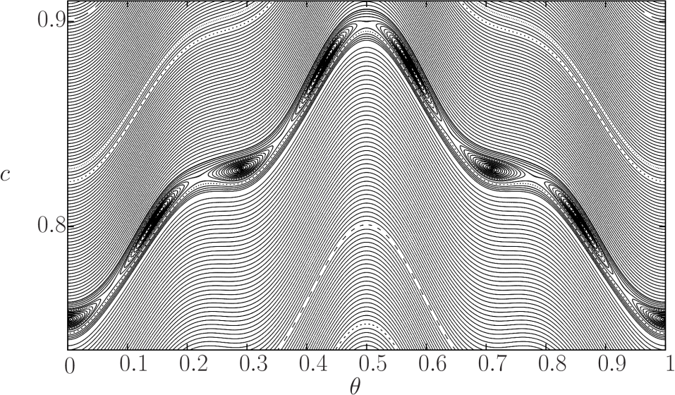
Figure 8: Blow up of the $7:3$ resonance labeled in Figure 4

\begin{picture}(1.0,0.5)\put(0.0,0.25){ \begin{@subfigure}\includegraphics[angle={-90},width=216.81pt]{eps6e-2_thetacw/inner_dynamics}\@@toccaption{{\lx@tag[ ]{{(a)}}{}}}\@@caption{{\lx@tag[ ]{{\footnotesize(a)}}{\footnotesize}}}\end{@subfigure} } \put(0.51,0.23){ \begin{@subfigure}\includegraphics[angle={-90},width=216.81pt]{with_spring/eps6e-2_xyc/inner_dynamics}\@@toccaption{{\lx@tag[ ]{{(b)}}{}}}\@@caption{{\lx@tag[ ]{{\footnotesize(b)}}{\footnotesize}}}\end{@subfigure} } \end{picture}

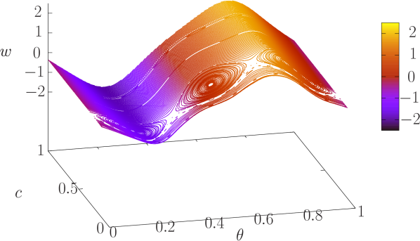
(a)

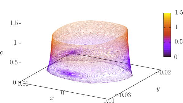
(b)

Figure 9: Dynamics restricted to the Normally Hyperbolic Manifold $\tilde{\mathcal{K}}_{\varepsilon}$ in the ambient space for the conservative case.

In Figure 9 we show the inner dynamics in the ambient space. In Figure 9(a) we show the variable $w$ parameterized by $\theta$ and $c$. Note that the amplitude of the oscillations performed by $w$ increase with $c$. These oscillations can be periodic or quasi-periodic depending on the dynamics of $\theta$-$c$. In Figure 9(b) we see the behaviour of $x$ and $y$. As sytems $\mathcal{X}$ and $\mathcal{U}$ are coupled through the Hamiltonian coupling $\varepsilon h$ (the spring), the saddle point $Q_{0}$ perturbs into an oscillatory motion.

As explained in Section 3, the Newton-like method reported in [19] also provides corrected versions of the normal bundle $N(\tilde{\mathcal{K}}_{\varepsilon})$ (the matrix $N_{\varepsilon}(\theta,c)$, see Section 3.1.2); that is, linear approximations of the parameterizations $W^{s,+}_{\varepsilon}$ and $W^{u,+}_{\varepsilon}$ given in Equations (17)-(18):

$$W^{s,+}(\theta,c,s,\tau,r) =\tilde{K}_{\varepsilon}(\theta,c,s)+(\tau,r)\cdot{\tilde{\Lambda}_{\varepsilon}^{S}(\theta,c)}+O(\tau^{2},r^{2},\tau r)$$ (43)

$$W^{u,+}(\theta,c,s,\tau) =\tilde{K}_{\varepsilon}(\theta,c,s)+\tau\cdot{\tilde{\Lambda}^{U}_{\varepsilon}(\theta,c)}+O(\tau^{2}),$$ (44)

where the matrices $\tilde{\Lambda}_{\varepsilon}^{S}$ and $\tilde{\Lambda}_{\varepsilon}^{U}$ (with dimensions $2\times 6$ and $1\times 6$) are the matrices $\Lambda_{\varepsilon}^{S}$ and $\Lambda_{\varepsilon}^{U}$ (having dimensions $5\times 2$ and $5\times 1$) transformed into coordinates $x,y,u,v,w,s$ and properly transposed.
When considering iterates of the linear approximations of the fibers of the points $\tilde{K}_{\varepsilon}(\theta,c,s)$ one obtains better approximations of the fibers of the corresponding inner iterates:

$$\mathcal{W}^{s,+}(f^{-n}(\theta,c),s) \simeq\tilde{K}_{\varepsilon}(f^{-n}(\theta,c),s)+\mathfrak{s}_{\varepsilon}^{-n}\left((\tau,r)\cdot{\tilde{\Lambda}_{\varepsilon}^{S}(\theta,c)}\right)$$ (45)

$$\mathcal{W}^{u,+}(f^{n}(\theta,c),s) \simeq\tilde{K}_{\varepsilon}(f^{n}(\theta,c),s)+\mathfrak{s}^{n}_{\varepsilon}\left(\tau\cdot{\tilde{\Lambda}^{U}_{\varepsilon}(\theta,c)}\right).$$ (46)

The higher $n$ and the smaller $\tau$ and $r$ are, the better the approximation is.

\begin{picture}(1.0,0.3)\put(0.0,0.0){ \begin{@subfigure}\includegraphics[width=216.81pt]{with_spring/bundle_matlab/normal_bundle_xy}\end{@subfigure} } \put(0.51,0.0){ \begin{@subfigure}\includegraphics[width=216.81pt]{with_spring/bundle_matlab/normal_bundle_xyc}\end{@subfigure} } \end{picture}

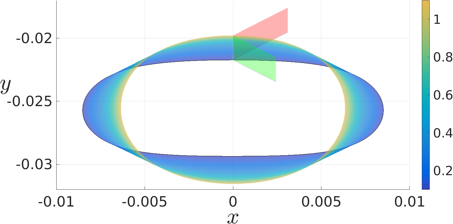
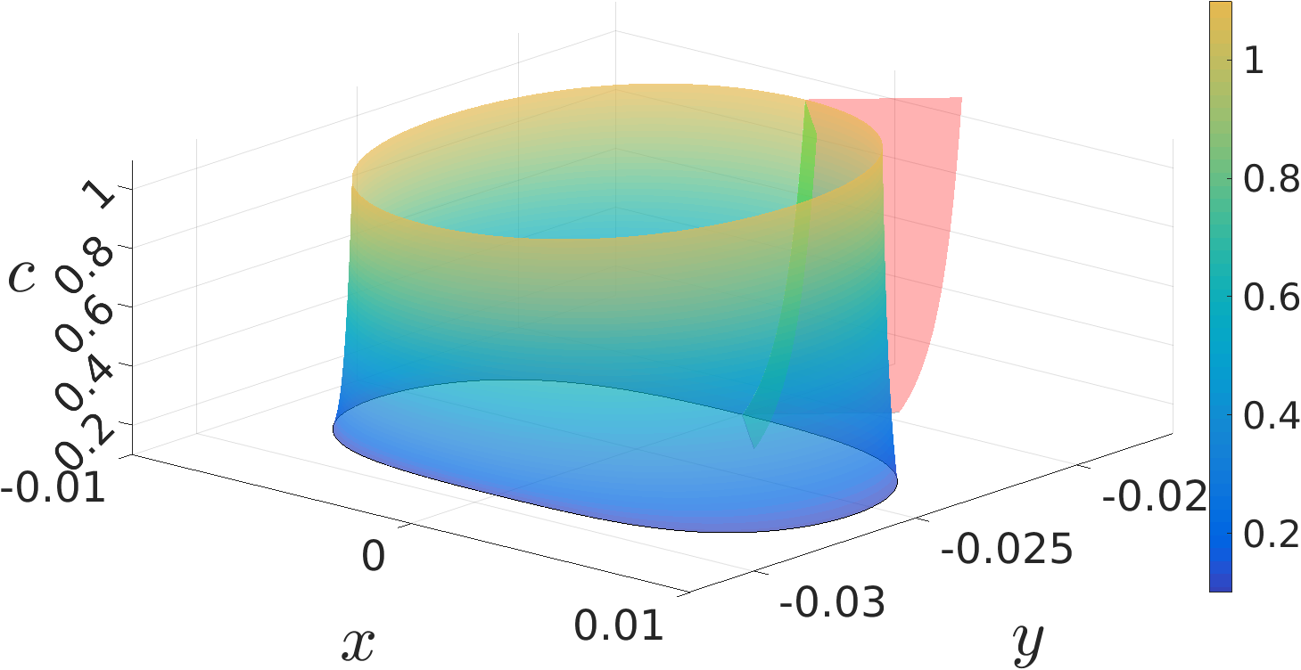
Figure 10: Normally Hyperbolic Manifold and its normal bundle $N(\tilde{\mathcal{K}}_{\varepsilon})$ for the conservative case: tangent space to the stable (green) and unstable (red) fiber for $\varepsilon=6\cdot 10^{-2}$, $\tilde{k}=1$, $\tilde{\zeta}=\tilde{\chi}=0$, $\theta=0.5$, $c\in[0.2,1.2]$, $r=0$ and $\tau\in[0,5\cdot 10^{-3}]$.

To illustrate this, we show in Figure 10 the $x-y-c$ projection of the normal bundle of a set of points given by $K_{\varepsilon}(\theta,c,s)$ with $\theta=0.5$, $c\in[0.1,1.2]$ $s=0$. For each such point we keep $r=0$ and slightly vary $\tau$, $\tau\in[0,5\cdot 10^{-3}]$, in Equations (43)-(44).

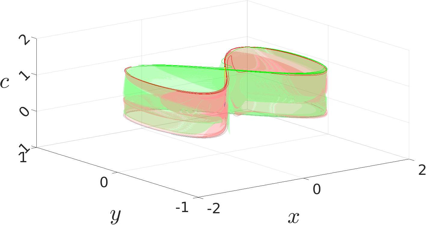
Figure 11: Iteration of the normal bundle shown in Figure 10. Green: $7$-th backwards iteration of the stable bundle. Red: $7$-th forwards iteration of the unstable bundle.

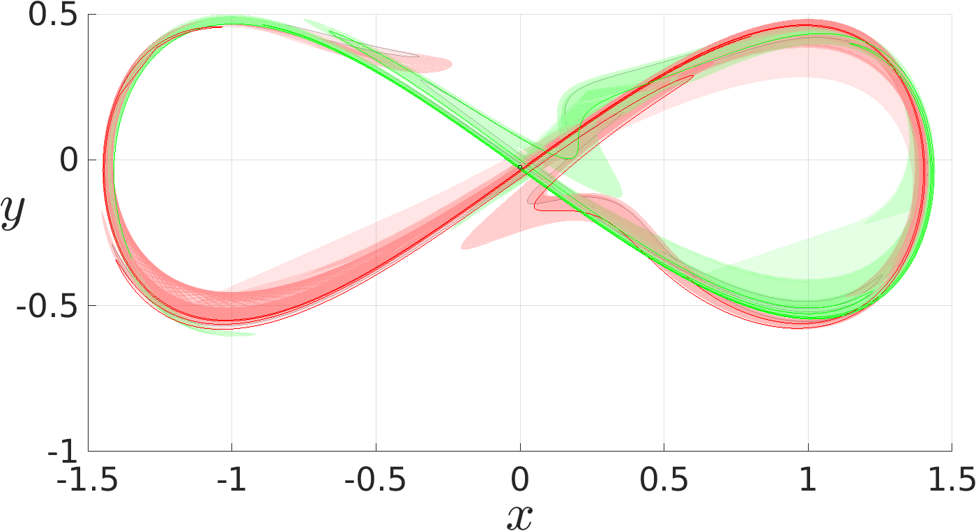
Figure 12: Projection in the $x-y$ plane of Figure 11.

In Figures 11 and 12 we show the global approximation of stable and unstable fibers by iterating $7$ times ($n=7$ in Equations (45)-(46)) the surfaces shown in Figure 10.
Figure 11 shows evidence of homoclinic intersections. Provided that the two beams are coupled by means of a conservative coupling (a spring), there is in this case hope to observe Arnold diffusion leading to $O(1)$ variations of the coordinate $c$. A study of homoclinic intersections, the Scattering map (see [8, 9]) and shadowing trajectories is left for future work.

Note that if the elastic constant of the spring is set to $\tilde{k}=0$, then the two beams remain uncoupled and the energy, $c$, of system $\mathcal{U}$ can only vary through the inner dynamics. Hence, in such a situation, homoclinic excursions do not inject extra energy to the beam represented by system $\mathcal{U}$. In other words, in this case, the Scattering map becomes the identity up to first order terms and there is no hope to observe Arnold diffusion in without the spring.

4.2 Dissipative case

4.2.1 Weak damping and conservative coupling

When adding small dissipation, hyperbolicity of the saddle periodic orbits guarantees their persistence for small enough dissipation. However, as shown in [25], when perturbed with dissipation, elliptic periodic orbits of area preserving maps become attracting foci.

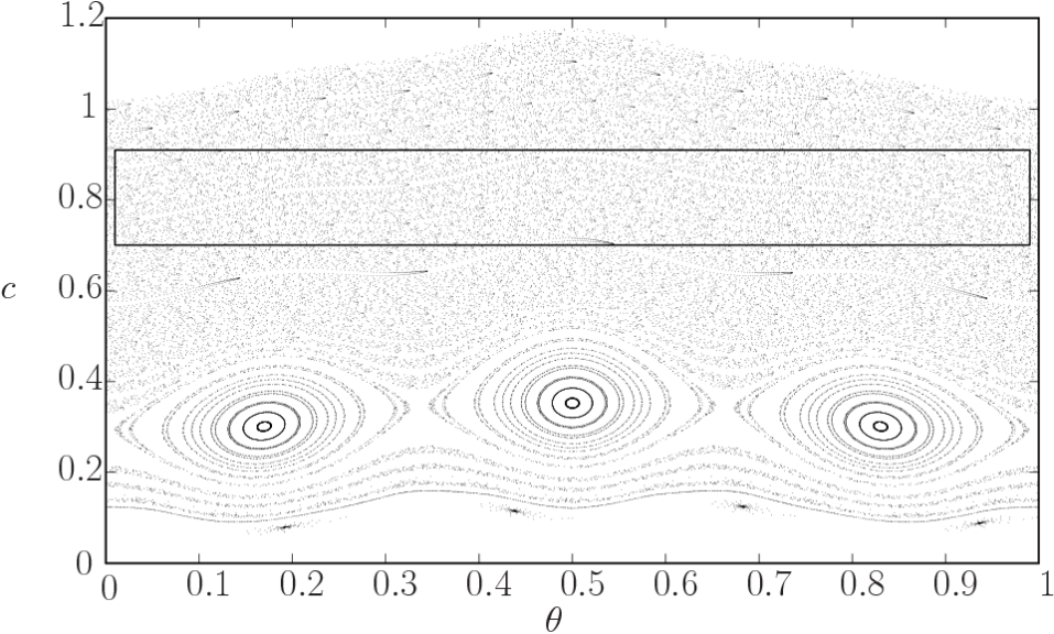
Figure 13: Inner dynamics in $\tilde{\mathcal{K}}_{\varepsilon}$ for weak damping: $\varepsilon=6\cdot 10^{-}2$, $\tilde{\zeta}=6\cdot 10^{-5}$ and $\tilde{\chi}=0$. We have taken $50$ initial conditions at $\theta=0.5$ and iterated them $1000$ times. The region labeled is maximized in Figure 14, where $400000$ iterations are used.

As shown in Figure 13, this occurs with $f_{\varepsilon}$ as well. There, $50$ initial conditions are taken at $\theta=0.5$ and iterated only $1000$ times for $\varepsilon=6\cdot 10^{-2}$, $\tilde{\chi}=0$, $\tilde{k}=1$ and $\tilde{\zeta}=6\cdot 10^{-5}$, which corresponds to an absolute magnitude of the damping coefficient of $\varepsilon\tilde{\zeta}=3.6\cdot 10^{-6}$. Some of them are attracted to the $3:1$ resonant focus, while others skip the separatrices of the saddle $3:1$ periodic orbit and are attracted to lower energy attractors.

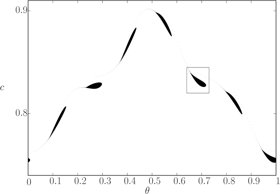
Figure 14: Approximated unstable manifold of the saddle periodic orbits corresponding to $7:3$ resonance under the presence of small damping: $\tilde{\chi}=0$, $\tilde{\zeta}=6\cdot 10^{-5}$, $\tilde{k}=1$ and $\varepsilon=6\cdot 10^{-2}$. The unstable manifold leaves the saddle point and rolls about the $7:3$ resonant attracting focus. The labeled region is magnified in Figure 15.

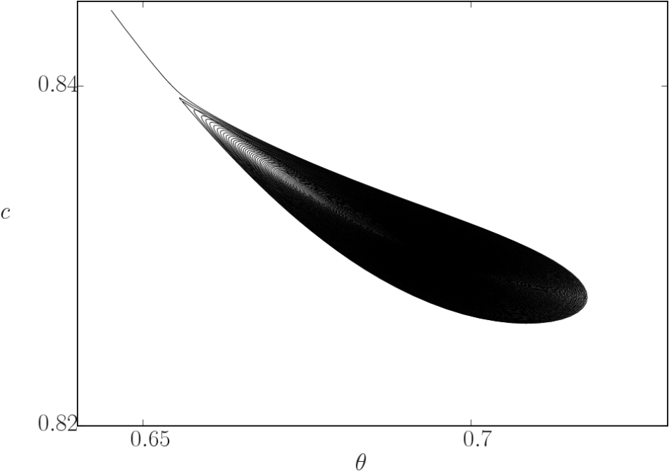
Figure 15: Blow up of the labeled region in Figure 14: unstable manifold of the $7:3$ resonant periodic orbit under weak damping.

In Figures 14 and 15 we show this in more detail for the $7:3$ resonant periodic orbits. There we have taken an initial condition very close to the unstable manifold of the saddle $7:3$ resonant periodic orbit. For forward iterates we see how this unstable manifold slowly rolls about the attracting focus while backwards iterates approach the saddle periodic orbit and rapidly scape due to limited numerical accuracy.

\begin{picture}(1.0,0.5)\put(0.0,0.32){ \begin{@subfigure} \includegraphics[angle={-90},width=216.81pt]{unstable_manifold_7-3_iterates_theta/inner_dynamics}\@@toccaption{{\lx@tag[ ]{{(a)}}{}}}\@@caption{{\lx@tag[ ]{{\footnotesize(a)}}{\footnotesize}}}\end{@subfigure} } \put(0.51,0.32){ \begin{@subfigure}\includegraphics[angle={-90},width=216.81pt]{unstable_manifold_7-3_iterates_c/inner_dynamics}\@@toccaption{{\lx@tag[ ]{{(b)}}{}}}\@@caption{{\lx@tag[ ]{{\footnotesize(b)}}{\footnotesize}}}\end{@subfigure} } \end{picture}

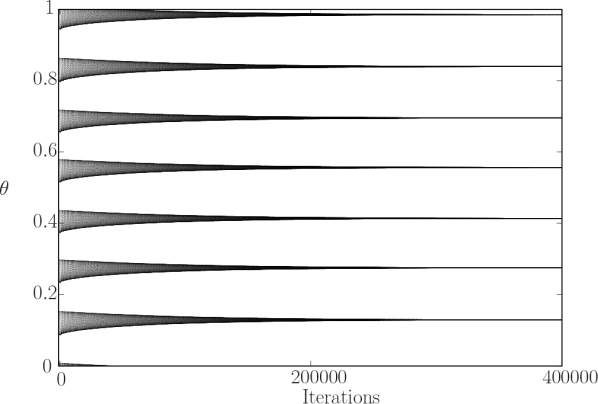
(a)

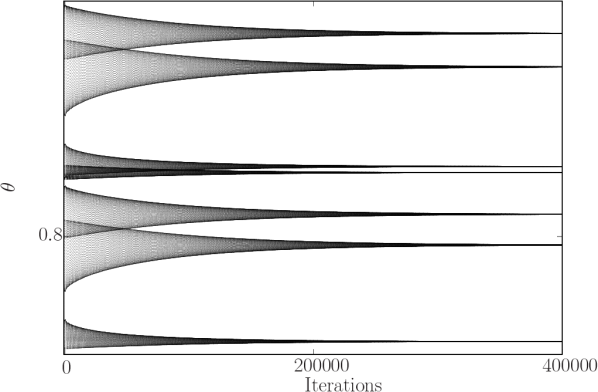
(b)

Figure 16: Iterates of $f_{\varepsilon}$ for the initial condition taken at the unstable manifold shown in Figure 14 and 15.

\begin{picture}(1.0,0.5)\put(0.0,0.32){ \begin{@subfigure} \includegraphics[angle={-90},width=216.81pt]{unstable_manifold_7-3_iterates_theta_zoom/inner_dynamics}\@@toccaption{{\lx@tag[ ]{{(a)}}{}}}\@@caption{{\lx@tag[ ]{{\footnotesize(a)}}{\footnotesize}}}\end{@subfigure} } \put(0.51,0.32){ \begin{@subfigure}\includegraphics[angle={-90},width=216.81pt]{unstable_manifold_7-3_iterates_c_zoom/inner_dynamics}\@@toccaption{{\lx@tag[ ]{{(b)}}{}}}\@@caption{{\lx@tag[ ]{{\footnotesize(b)}}{\footnotesize}}}\end{@subfigure} } \end{picture}

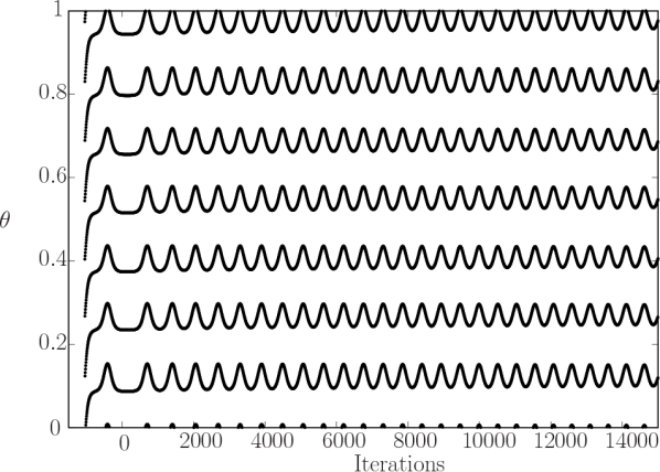
(a)

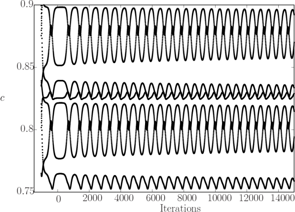
(b)

Figure 17: First iterates of $f_{\varepsilon}$ and $f_{\varepsilon}^{-1}$ for the initial condition taken at the unstable manifold shown in Figures 14 and 15.

This is better appreciated in Figures 16 and 17, where we show the “time” evolution of $\theta$ and $c$, both forwards and backwards in time.

The dissipation exhibited by the inner dynamics is indeed not desired from the applied point of view, as it implies convergence to lower energy oscillatory regimes providing lower amplitude alternate voltage for variable $w$, which is the voltage provided to the load connected to the harvesting beams (see Figure 2(b)). As mentioned in the Introduction, one of the purposes of this work is to provide tools that can prevent or slow down this loss of energy, such as the ones based on outer excursions through homoclinic intersections. We therefore are interested on studying the manifold $\tilde{\mathcal{K}}_{\varepsilon}$ and its stable and unstable manifolds for the dissipative case.

Regarding the computations of these manifolds, we obtained results very similar to those reported for the conservative case in Section 4.1. That is, in the ambient space, the manifold $\tilde{\mathcal{K}}_{\varepsilon}$ and the normal bundle look very similar to those shown in Figures 9 and 10, respectively. Moreover, when iterating the normal bundle, we obtain global fibers similar to the ones shown in Figures 10 and 11. As the homoclinic intersections shown for the conservative case in Section 4.1 are transversal, they are robust to perturbations, even dissipative ones. Hence, we also observe evidence of homoclinic connections allowing one to define the Scattering map. Due to the (conservative) coupling, the Scattering map may possess $O(\varepsilon)$ terms in the action $c$, although expressions for this map for dissipative cases have not been reported anywhere. Hence, through homoclinic excursions, one may inject $O(\varepsilon)$ into the system which may help slowing down the dissipation observed in the inner dynamics. However, Arnold diffusion is rather unlikely to exist due to the presence of dissipation.

4.2.2 Full system

We now present the numerical results for the full case: $\tilde{k},\tilde{\zeta},\tilde{\chi}>0$.
In comparison with the previous case of Section 4.2.1, we now add the extra dissipative coupling term given by the coupling piezoelectric effect: $\tilde{\chi}>0$. Regarding the inner dynamics, computations reveal that, as one would expect, the effect is similar to the situation given in Section 4.2.1 when the dissipation was only due to the damping on the oscillators. We observe that the parameter $\tilde{\chi}$ seems to contribute less than $\tilde{\zeta}$ in destroying objects due to dissipation.

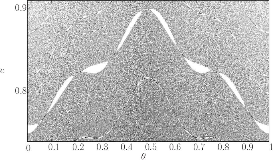
Figure 18: Inner dynamics around the 7:3 resonant attracting focus for $\varepsilon=6\cdot 10^{-2}$, $\tilde{\zeta}=6\cdot 10^{-5}$ and $\tilde{\chi}=10^{-4}$.

In Figure 18 we show how the $7:3$ resonant saddle and focus periodic orbits still persist for $\tilde{\chi}=10^{-4}$.

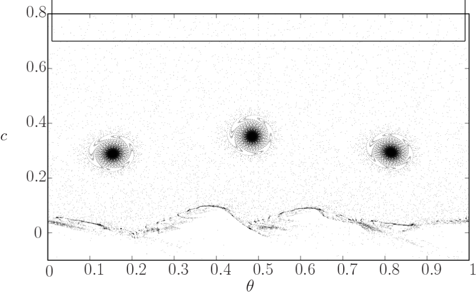
Figure 19: Inner dynamics for $\varepsilon=6\cdot 10^{-2}$, $\tilde{\zeta}=6\cdot 10^{-5}$ and $\tilde{\chi}=2\cdot 10^{-1}$.

As shown in Figure 19, for larger values of $\tilde{\chi}$, periodic orbits bifurcate and most initial conditions are attracted towards a low energy attractor. For $\tilde{\chi}=2\cdot 10^{-1}$, the $3:1$ resonant periodic attracting focus still exists.

\begin{picture}(1.0,0.5)\put(0.0,0.32){ \begin{@subfigure} \includegraphics[angle={-90},width=216.81pt]{only_coupling/resonance_3-1_iterates_theta/inner_dynamics}\@@toccaption{{\lx@tag[ ]{{(a)}}{}}}\@@caption{{\lx@tag[ ]{{\footnotesize(a)}}{\footnotesize}}}\end{@subfigure} } \put(0.51,0.32){ \begin{@subfigure}\includegraphics[angle={-90},width=216.81pt]{only_coupling/resonance_3-1_iterates_c/inner_dynamics}\@@toccaption{{\lx@tag[ ]{{(b)}}{}}}\@@caption{{\lx@tag[ ]{{\footnotesize(b)}}{\footnotesize}}}\end{@subfigure} } \end{picture}

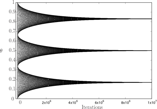
(a)

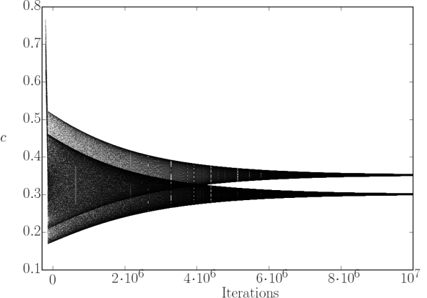
(b)

Figure 20: Iterates by $f_{\varepsilon}$ and $f_{\varepsilon}^{-1}$ of an initial condition attracted by the $3$-periodic focus.

Iterates of $f_{\varepsilon}$ and $f^{-1}_{\varepsilon}$ close to the $3:1$ attracting focus are shown in Figure 20(a). Backwards iterates are also shown until the trajectory scapes.

The manifold $\tilde{K}_{\varepsilon}$ in the ambient space and its normal bundle $N(\tilde{K}_{\varepsilon})$ look very similar to the conservative case considered in Section 4.1 (Figures 9 and 10). We therefore omit including including similar figures. However, in this case we also show the $7th$ iterate of the normal bundle in Figures 21 and 22. As one can see there, for the chosen parameter values, there still exists evidence of existence of intersections between the stable and unstable manifolds leading to homoclinic connections. Hence, we show that there is hope that, through these homoclinic connections, outer excursions can inject energy to the beam defined by Hamiltonian $\mathcal{U}$ that may help the system slow down the loss of energy shown by the inner dynamics previously discussed.

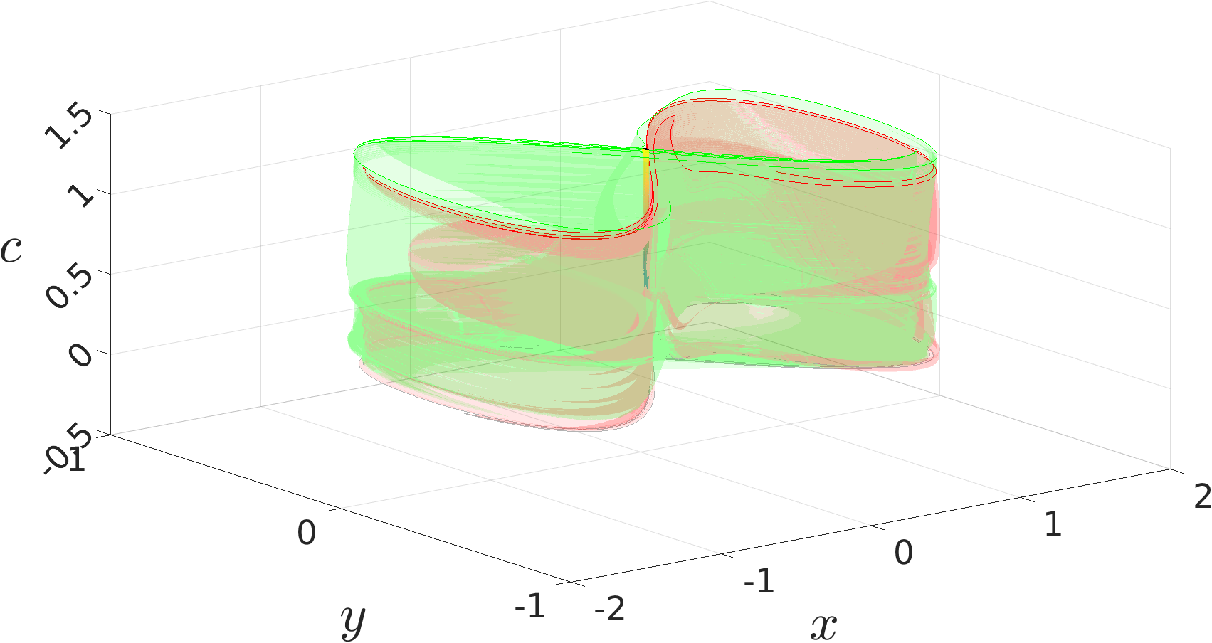
Figure 21: Stable and unstable fibers of

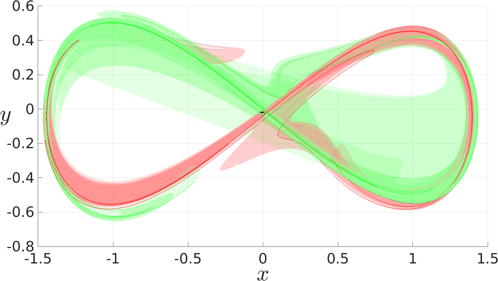
Figure 22: Projection to the $x-y$ plane of Figure 21

5 Conclusions

This paper is a first step towards the use of theory related to Arnold diffusion in energy harvesting systems based on bi-stable oscillators, such as piezoelectric beams or cantilevers. Such theory could be extremely useful in this field, as it precisely deals with the accumulation of energy in oscillators absorbed from a given periodic source.
The dynamics of such systems is given by the coupling of periodically forced Duffing oscillators. The coupling is given by an extra variable (a voltage) which at the same time adds extra dissipation to the intrinsic damping. Moreover, this coupling adds and extra dimension to the system. The goal of this work is to provide a theoretical and numerical background to study the existence and persistence of Normally Hyperbolic Manifolds and the intersection between their unstable and stable manifolds. Such intersections are the basis of the so-called “outer dynamics” in Arnold diffusion theory. Through these intersections, the system may increase its energy by absorbing energy from the source, which is studied by the “Scattering” map. To benefit higher order of energy abortion, we have proposed to add to the system an extra conservative coupling given by a spring. In the absence of damping and the piezoelectric dissipative coupling, this extra coupling could allow the presence of Arnold diffusion when periodically forced.

In the absence of forcing, damping and both couplings, we have proven the existence of a $3$-dimensional Normally Hyperbolic Invariant Manifold with $5$ and $6$-dimensional unstable and stable manifolds. The unperturbed manifold possesses boundaries; despite the system’s dissipation, it persists and is unique. However, in the presence of dissipation, the inner dynamics becomes unbounded and hence the manifold needs to be non-uniquely extended beyond the original boundaries.

By implementing the Parameterization method we have computed this manifold, its inner dynamics and good approximations of its stable and unstable manifolds. We have numerically investigated three different situations.
In the absence of damping and dissipative coupling, but including the conservative one, the inner dynamics is given by a symplectic map. The stable and unstable manifolds intersect, giving rise to outer excursions through homoclinic intersections. In this case, the Scattering map could be properly defined, and first order terms could be computed as usual.
When the damping is enabled, the inner dynamics is not given by an area preserving map anymore. Instead, the inner dynamics at the manifold possesses global attractors to which trajectories are attracted losing energy. However, we have shown evidence of existence of homoclinic connections. Such intersections may lead to outer excursions injecting energy, which could be used to overcome or slow down the loss of energy given at inner dynamics. This is extremely desired from the applied point of view and may help to optimize energy harvesting systems based on this type of oscillators. However, the system may not exhibit Arnold diffusion anymore due to the presence of dissipation.
We have finally numerically studied the full system, and shown that a similar situation applies up to higher values of the piezoelectric coupling.

We propose to continue our work by providing a theoretical background for the existence of homoclinic intersections (Melnikov theory) and the Scattering map for dissipative systems, on one hand. On the other hand, we also propose an accurate numerical computation of homoclinic intersections and the Scattering map, in order to quantify the amount of absorbed energy from the source.

References

- [1] V. I. Arnol’d. Instability of dynamical systems with several degrees of freedom. Sov. Math. Doklady, 5:581–585, 1964.
- [2] P. Bernard, V. Kaloshin, and K. Zhang. Arnol’d diffusion in arbitrary degrees of freedom and 3-dimensional normally hyperbolic invariant cylinders. Acta Mathematica, 2016. To appear.
- [3] X. Cabré, E. Fontich, and R. de la Llave. The parameterization method for invariant manifolds I: Manifolds associated to non-resonant subspaces. Indiana Univ. Math. J., 52:283–328, 2003.
- [4] X. Cabré, E. Fontich, and R. de la Llave. The parameterization method for invariant manifolds II: Regularity with respect to parameters. Indiana Univ. Math. J., 52:329–360, 2003.
- [5] X. Cabré, E. Fontich, and R. de la Llave. The parameterization method for invariant manifolds III: overview and applications. J. Diff. Eqts., 218:444–515, 2005.
- [6] R. Calleja, A. Celletti, and R. de la Llave. A KAM theory for conformally symplectic systems: Efficient algorithms and their validation. Journal of Differential Equations, 255:978–1049, 2013.
- [7] R. de la Llave. A tutorial on KAM theory. http://www.ma.utexas.edu/mp_arc-bin/mpa?yn=01-29, 2000.
- [8] A. Delshams, R. de la Llave, and T.M. Seara. A geometric mechanism for diffusion in hamiltonian systems overcoming the large gap problem: Heuristics and rigorous verification on a model. Memoirs of the American Mathematical Society, 179, 2006.
- [9] A. Delshams, R. de la Llave, and T.M. Seara. Geometric properties of the scattering map of a normally hyperbolic invariant manifold. Adv. in Math., 217(3):1096–1153, Febraury 2008.
- [10] A. Ertuk, J. Hoffman, and D.J. Inman. A piezomagnetoelastic structure for broadband vibration energy harvesting. Applied Physics Letters, 94, 2009.
- [11] A. Erturk and D.J. Inman. An experimentally validated bimorph cantilever model for piezoelectric energy harvesting from base excitations. Smart Mater. Struct., 19, 2009.
- [12] A. Erturk, J.M. Renno, and D.J. Inman. Modeling of Piezoelectric Energy Harvesting from an L-saped Beam-mass Stucture with an Application to UAVs. Journ. Intell. Mat. Systs. Struc., 20, 2009.
- [13] J. Féjoz, M. Guàrdia, V. Kaloshin, and P. Roldán. Kirkwood gaps and diffusion along mean motion resonances in the restricted planar three-body problem. Jour. Europ. Math. Soc., 2016. To appear.
- [14] N. Fenichel. Persistence and smoothness of invariant manifolds for flows. Indiana Univ. Math. J., 21:193–226, 1971/1972.
- [15] M. Ferrari, V. Ferrari, M. Guizzetti, B. Andó, S. Baglio, and C. Trigona. Improved energy harvesting from wideband vibrations by nonlinear piezoelectric converters. Procedia Chemistry, 1(1):1203–1206, 2009.
- [16] M. Gidea, R. de la Llave, and T.M. Seara. A General Mechanism of Diffusion in Hamiltonian Systems: Qualitative Results. Preprint available at http://http://arxiv.org/abs/1405.0866, 2014.
- [17] A. Granados, S.J. Hogan, and T.M. Seara. The scattering map in two coupled piecewise-smooth systems, with numerical application to rocking blocks. Physica D, 269:1–20, 2014.
- [18] J. Guckenheimer and P. J. Holmes. Nonlinear Oscillations, Dynamical Systems and Bifurcations of Vector Fields. Appl. Math. Sci. Springer, 4th edition, 1983.
- [19] Àlex Haro, Marta Canadell, Josep-Lluís Figueras, Alejandro Luque, and Josep-Maria Mondelo. The Parameterization Method for Invariant Manifolds: From Rigorous Results to Effective Computations. Springer, 2016.
- [20] I.-H. Kim, H.J. Jung, B.M. Lee, and S.J. Jang. Broadband energy-harvesting using a two degree-of-freedom vibrating body. Appl. Phys. Lettrs., 98, 2011.
- [21] G. Litak, M.I. Friswell, C.A. Kitio Kwuimy, S. Adhikari, and M. Borowiec. Energy harvesting by two magnetopiezoelastic oscillators. Proceedings of the XI conference on Dynamical Systems, Theory and Applications, Lódź December 2011, 2011.
- [22] A. Luque and D. Peralta-Salas. Arnold diffusion of charged particles in ABC magnetic fields. Preprint available at http://arxiv.org/abs/1509.04141, 2015.
- [23] J.-P. Marco. Arnold diffusion for cusp-generic nearly integrable systems on . Preprint available at http://arxiv.org/abs/1602.02403, 2014.
- [24] F.C Moon and P.J. Holmes. A magnetoelastic strange attractor. Journal of Sound and Vibration, 65:275–296, 1979.
- [25] C. Simó and A. Vieiro. Planar radial weakly dissipative diffeomorphisms. Chaos, 20, 2010.
- [26] S.C. Stanton, B.A.M. Owens, and B.P. Mann. Harmonic balance analysis of the bistable piezoelectric inertial generator. Journ. Sound Vibr., 331:3617–3627, 2012.
- [27] H. Vocca, I. Neri, F. Travasso, and L. Gammaitoni. Kinetic energy harvesting with bistable oscillators. Applied Energy, 97:771–776, 2012.