Second-order perturbation theory for ${}^{3}\mathrm{He}$ and $pd$ scattering
in pionless EFT

Abstract

This work implements pionless effective field theory with the two-nucleon system expanded around the unitarity limit at second-order perturbation theory. The expansion is found to converge well. All Coulomb effects are treated in perturbation theory, including two-photon contributions at next-to-next-to-leading order. After fixing a three-nucleon force to the ${}^{3}\mathrm{He}$ binding energy at this order, proton-deuteron scattering in the doublet S-wave channel is calculated for moderate center-of-mass momenta.

I Introduction

Effective field theory (EFT) is an established tool in theoretical nuclear physics to connect the description of nuclei in terms of hadronic degrees of freedom to the underlying physics of quantum chromodynamics (QCD). In relying only on basic concepts—symmetries, the separation of scales, and a systematic ordering of contributions—it is both elegant and pragmatic at the same time. While the most widely used framework used for the description of nuclear structure and reactions is based on the approximate (and spontaneously broken) chiral symmetry of the QCD, for momentum scales well below the pion mass $M_{\pi}$, pion-exchange contributions cannot be resolved explicitly. The resulting pionless EFT contains, besides electromagnetic forces, only contact interactions between nonrelativistic fields Bedaque:1997qi; vanKolck:1997ut; Kaplan:1998tg; Bedaque:1998mb; Kaplan:1998we; Birse:1998dk; vanKolck:1998bw; Chen:1999tn; Bedaque:1999vb; Gabbiani:1999yv. From the original chiral symmetry it only keeps the isospin subgroup as an approximate symmetry.

This, however, is not the primary driving feature of the theory. Instead, the fact that the $NN$ S-wave scattering lengths—$5.4$ (${-}23.7$) $\mathrm{fm}$ in the ${}^{3}S_{1}$ (${}^{1}S_{0}$) channel—happen to be large compared to the typical scale $M_{\pi}^{-1}\sim 1.4\leavevmode\nobreak\ \mathrm{fm}$ implies that the few-nucleon sector is close to a universal regime where short-range details have little impact on low-energy parameters. In the two-nucleon sector, this is manifest in the effective range expansion (ERE) working as well as it does Bethe:1949yr. In the three-nucleon sector, the spin-doublet S-wave configuration is governed by a non-derivative three-body interaction at leading order (LO) Bedaque:1999ve; Hammer:2000nf; Hammer:2001gh; Bedaque:2002yg; Afnan:2003bs; Griesshammer:2005ga, and the theory, formally equivalent to one for three bosons with short-range interactions, describes the triton as an approximate Efimov state Efimov:1970zz; Efimov:1981aa; Hammer:2010kp. For a recent review of the pionless three-body calculations, see Ref. Vanasse:2016jtc.

An important feature of the theory is that it can be constructed in a way such that it is fully renormalized order by order, with all nonperturbative effects included at LO and the rest treated in perturbation theory Hammer:2001gh; Vanasse:2013sda; Konig:2013cia; Vanasse:2014kxa; Konig:2015aka. This allows for precise calculations of low-energy observables with controlled error estimates based directly on the EFT expansion and independent of working at a fixed or limited regulator scale. Recent examples of high-order calculations can be found in Refs. Margaryan:2015rzg; Vanasse:2015fph). Moreover, pionless EFT provides a controlled “laboratory” to study such perturbative schemes (expanding directly the amplitude instead of a potential), which have been argued to be important for chiral EFT as well (see for example Refs. Long:2016ybt; Valderrama:2016koj for recent reviews).

While electromagnetic effects are certainly important for a realistic description of nuclei, their inclusion into the EFT provides a challenge because the long-range nature of these forces—meaning that the Coulomb force becomes dominant at very low energies, precisely where the short-range expansion otherwise works best—is not easily accommodated in the power counting. Early work on Coulomb effects in the $pp$ Kong:1998sx; Kong:1999sf; Kong:2000px; Butler:2001jj; Barford:2002je; Ando:2007fh; Ando:2008va; Ando:2008jb and $pd$ Rupak:2001ci systems was followed up on in Refs. Ando:2010wq; Konig:2011yq, with the latter providing a first calculation of $pd$ doublet-channel scattering.

It has become clear that if perturbative renormalization is to be maintained, including electromagnetic effects is not as simple as adding a Coulomb potential to the short-range terms, as it is typically done in calculations based on effective pionless potentials Kirscher:2009aj; Kirscher:2011uc; Kirscher:2011zn; Lensky:2016djr. Based on studying the regulator (cutoff) dependence of the amplitude, it was realized that in the presence of nonperturbative Coulomb effects an isospin breaking three-nucleon force is required to ensure renormalization at next-to-leading order (NLO) Vanasse:2014kxa; Konig:2014ufa. While another calculation Kirscher:2015zoa does not see the need to include such a term, Ref. Konig:2015aka showed that in part this three-body force is related to a two-body divergence in the $pp$ sector, and that the theory can be rearranged in such a way that all Coulomb effects in the ${}^{3}\mathrm{He}$ bound state are included in perturbation theory. In this counting the ${}^{1}S_{0}$ channel is taken in the unitarity limit (infinite scattering length) at LO and the effects of the finite physical scattering lengths—$a_{t}$ as given above as well as the Coulomb-modified $pp$ scattering $a_{C}\simeq 7.81\leavevmode\nobreak\ \mathrm{fm}$—are accounted for by parameters entering at NLO. In particular, in the $pp$ channel this parameter absorbs the logarithmic divergence generated by one-photon exchange in the two-nucleon subsystem. Demoting all other (small) isospin-breaking effects to next-to-next-to-leading order (N${}^{2}$LO) or higher, Ref. Konig:2015aka was able to calculate the ${}^{3}\mathrm{H}$–${}^{3}\mathrm{He}$ binding-energy difference at NLO without a new three-nucleon force. More generally, this scheme enhances the predictive power of the theory by making the ${}^{1}S_{0}$ channel parameter free at LO.

More recent work Konig:2016utl goes further and considers a more radical expansion that takes the ${}^{3}S_{1}$ scattering length to infinity as well in a “full unitarity” leading order, whereas Ref. Vanasse:2016umz explores similar ideas by expanding around a leading order that exhibits the $SU(4)_{W}$ spin-isospin symmetry Wigner:1936dx for finite scattering lengths.

In this work, the pionless unitarity-LO counting schemes developed in Refs. Konig:2015aka; Konig:2016utl are implemented up to N${}^{2}$LO, including effects from two-photon exchange and other isospin-breaking corrections. It thereby establishes the convergence of these expansions up to this order. Going beyond NLO (first-order perturbation theory), where all corrections enter linearly, is an important proof of principle. Moreover, it is demonstrated explicitly that away from the zero-energy threshold it is possible to describe $pd$ scattering with fully perturbative Coulomb effects. Finally, it establishes the presence of an N${}^{2}$LO three-body force, to be fixed by a single $pd$ doublet datum, at N${}^{2}$LO.

After discussing the basic setup and contributions—most notably two-photon diagrams—in Sec. II, the perturbative calculation of three-body observables is described in Sec. III. Results are presented and discussed in Sec. LABEL:sec:Results, followed by a conclusion and outlook in Sec. LABEL:sec:Conclusion. Some details left out from the main text are provided in an appendix.

II Formalism and building blocks

This section collects the ingredients required to set up the N${}^{2}$LO calculation, summarizing results from previous works as far as necessary to make the current description reasonably self-contained.

II.1 Effective Lagrangian and dibaryon propagators

Using the notation of Ref. Konig:2015aka, the effective Lagrangian is split into one-, two- and three-body terms according to

$$\mathcal{L}=N^{\dagger}\left(\mathrm{i}D_{0}+\frac{\boldsymbol{D}^{2}}{2M_{N}}\right)N+\mathcal{L}_{\mathrm{2d}}+\mathcal{L}_{\mathrm{2t}}+\mathcal{L}_{3}\,,$$ (3)

where $N$ is the nonrelativistic nucleon field (doublet in spin and isospin space), coupled to (Coulomb) photons with the covariant derivative $D_{\mu}=\partial_{\mu}+\mathrm{i}eA_{\mu}\hat{Q}_{N}$ (with charge operator $\hat{Q}_{N}=(1+\tau_{3})/2$). The $NN$ S-wave two-body interactions are conveniently expressed in terms of auxiliary dibaryon fields $d^{i}$ (${}^{3}S_{1}$) and $t^{A}$ (${}^{1}S_{0}$), where $i$ and $A$ are spin-1 and isospin-1 indices, respectively. The corresponding Lagrangians are

$$\mathcal{L}_{\mathrm{2d}}=-d^{i\dagger}\left[\sigma_{d}+c_{d}\left(\mathrm{i}D_{0}+\frac{\boldsymbol{D}^{2}}{4M_{N}}\right)\right]d^{i}+y_{d}\left[d^{i\dagger}\left(N^{T}P^{i}_{d}N\right)+\mathrm{h.c.}\right]\,,$$ (4)

with the repeated superscripts $i$ summed over, and

$$\mathcal{L}_{\mathrm{2t}}=-t^{0\dagger}\left[\sigma_{t}+c_{t}\left(\mathrm{i}D_{0}+\frac{\boldsymbol{D}^{2}}{4M_{N}}\right)\right]t^{0}-t^{{-1}\dagger}\left[\sigma_{t,pp}+c_{t,pp}\left(\mathrm{i}D_{0}+\frac{\boldsymbol{D}^{2}}{4M_{N}}\right)\right]t^{-1}\\ -t^{{+1}\dagger}\left[\sigma_{t,nn}+c_{t,nn}\left(\mathrm{i}D_{0}+\frac{\boldsymbol{D}^{2}}{4M_{N}}\right)\right]t^{+1}+y_{t}\left[t^{{\tilde{A}}\dagger}\left(N^{T}\tilde{P}^{\tilde{A}}_{t}N\right)+\mathrm{h.c.}\right]\,.$$ (5)

Note that the ${}^{1}S_{0}$ part is separated into physical channels ($np$, $nn$, $pp$). Further details, including the projection operators $P^{i}_{d}$ and $\tilde{P}^{\tilde{A}}_{t}$ can be found in Ref. Konig:2015aka. Setting $y_{d}^{2}=y_{t}^{2}=4\pi/M_{N}$, the remaining low-energy constants $\sigma_{d/t(,\cdot\cdot)}$ and $c_{d/t(,\cdot\cdot)}$ correspond directly to the scattering lengths and effective ranges in the respective channel. Contributions from the $NN$ shape parameters first enter at N${}^{3}$LO Margaryan:2015rzg in the standard pionless power counting so that they also do not have to be included in the calculations presented here.

In the well-known fashion, nucleon-bubble insertions into the bare dibaryon propagators are resummed to obtain the full leading-order expressions

$$\mathrm{i}\Delta_{d/t(,\cdot\cdot)}^{(0)}(p_{0},\mathbf{p})=\frac{-\mathrm{i}}{\sigma_{d/t(,\cdot\cdot)}^{(0)}+y_{d/t(,\cdot\cdot)}^{2}I_{0}(p_{0},\mathbf{p})}\,,$$ (6)

where

$$I_{0}(p_{0},\mathbf{p})=M_{N}\int^{\Lambda}\!\!\frac{\mathrm{d}^{3}q}{(2\pi)^{3}}\frac{1}{M_{N}p_{0}-\mathbf{p}^{2}/4-\mathbf{q}^{2}+\mathrm{i}\varepsilon}\\ ={-}\frac{M_{N}}{4\pi}\left(\frac{2\Lambda}{\pi}-\sqrt{\frac{\mathbf{p}^{2}}{4}-M_{N}p_{0}-\mathrm{i}\varepsilon}\right)+\mathcal{O}(1/\Lambda)$$ (7)

is the generic nucleon bubble integral (Green’s function from zero to zero separation) calculated with a sharp momentum cutoff.

In principle, an S-D mixing operator in the ${}^{3}S_{1}$ channel enters at N${}^{2}$LO. However, at this order it does not contribute to the ${}^{3}\mathrm{H}$–${}^{3}\mathrm{He}$ binding energy splitting, and neither is it relevant for the doublet S-wave phase shift Vanasse:2013sda. Hence, it is not necessary to consider this operator in the present work. Moreover, terms stemming from relativistic corrections and transverse photons are suppressed by inverse powers of $M_{N}$ and do thus not contribute to the order considered in this paper.

II.1.1 Power counting around the unitarity limit

In the power counting developed in Ref. Konig:2015aka, which is applied here up to N${}^{2}$LO, the usual pionless expansion in terms of $Q/\Lambda_{\not{\pi}}$, where $Q$ denotes the typical momentum of the process under consideration and $\Lambda_{\not{\pi}}\sim M_{\pi}$ is the pionless breakdown scale, is paired with an additional expansion in $\aleph_{0}/Q$, where

$$\aleph_{0}\sim\alpha M_{N}\sim 1/|a_{t}|\sim 1/|a_{C}|$$ (8)

is a typical low-energy scale in the ${}^{1}S_{0}$ channel. This combines the inverse scattering lengths with the typical Coulomb scale $\alpha M_{N}$. In particular, at leading order the ${}^{1}S_{0}$ channel is considered in the unitarity limit (where the scattering lengths are infinite) and thus also isospin symmetric. The expansion in $\aleph_{0}/Q$ then corresponds to including the effects of finite $1/a_{t}$ and $1/a_{C}$ in perturbation theory, where the latter is naturally paired with one-photon exchange and ensures consistent renormalization in the presence of Coulomb effects. Range corrections reflect the $Q/\Lambda_{\not{\pi}}$ expansion, as in the standard pionless counting. Details of how the expansion is implemented by fixing the dibaryon parameters are given in Sec. II.5.

This scheme is constructed for the regime $\aleph_{0}\ll Q\ll\Lambda_{\not{\pi}}$, which naturally includes the ${}^{3}\mathrm{He}$ bound states. This was studied in Ref. Konig:2015aka, which also found that the $\aleph_{0}/Q$ expansion works well in the $nd$ scattering system. In $pd$ scattering, Coulomb effects are certainly nonperturbative at very small center-of-mass momenta ($k\to 0$), but for larger $k$ (determining $Q$ in this case), the perturbative expansion should work as well. This is demonstrated in the present work.

More generally, the scheme of Ref. Konig:2015aka counts isospin-breaking corrections, not only of electromagnetic origin but also those induced by the up-down quark-mass difference in QCD. As required by renormalization, the effects that give rise $a_{C}\neq a_{t}$ to are accounted for at NLO together with electromagnetic contributions. Different values have been determined for the $nn$ scattering length GonzalezTrotter:2006wz; Huhn:2001yk, but it is generally assumed large (and negative), such that $1/a_{t,nn}\approx 1/a_{t}$. Following the counting of Ref. Konig:2015aka, this difference is accounted for here by an N${}^{2}$LO correction, and for definiteness the central value favored by the pionless analysis of Ref. Kirscher:2011zn, $a_{t,nn}\simeq{-}(22.9\pm 4.1)\leavevmode\nobreak\ \mathrm{fm}$, is adopted here. The small isospin breaking in the effective ranges, $r_{C}-r_{t}\simeq 0.06\leavevmode\nobreak\ \mathrm{fm}$ is also included at N${}^{2}$LO.

Recently, Ref. Konig:2016utl suggested a more radical rearrangement of the power counting that includes the ${}^{3}S_{1}$ inverse scattering length $1/a_{d}$ in $\aleph_{0}$ instead of counting it as $\mathcal{O}(Q)$ (which is done in the standard pionless counting). Although this expansion only perturbatively moves the deuteron bound state—which at LO is located at zero energy in this expansion—to its physical position, Ref. Konig:2016utl found that it works well for three and four-nucleon bound states at NLO. As part of this work, ${}^{3}\mathrm{He}$ is considered up to second order in this “full unitarity” scheme.

II.1.2 Three-nucleon forces

It is well known that in pionless EFT a three-nucleon interaction is needed already at LO to ensure renormalization of the doublet-channel amplitude Bedaque:1999ve. This piece can be written as Ando:2010wq; Griesshammer:2011md

$$\mathcal{L}_{3,\text{LO}}=\frac{h}{3}N^{\dagger}\left[y_{d}^{2}\,d^{i\dagger}d^{j}\sigma^{i}\sigma^{j}+y_{t}^{2}\,t^{A\dagger}t^{B}\tau^{A}\tau^{B}-y_{d}y_{t}\left(d^{i\dagger}t^{A}\sigma^{i}\tau^{A}+\mathrm{h.c.}\right)\right]N\,,$$ (9)

where the coupling $h$ is also split up in various orders, with each piece having a characteristic log-periodic dependence on the momentum cutoff $\Lambda$ that is used in the three-body integral equations:

$$h=\frac{2H_{0,0}(\Lambda)}{\Lambda^{2}}+\frac{2H_{0,1}(\Lambda)}{\Lambda^{2}}+\frac{2H_{0,2}(\Lambda)}{\Lambda^{2}}+\cdots\,.$$ (10)

In addition to this, Ref. Ji:2012nj firmly established (for the analogous three-boson system) that an additional energy-dependent three-body force enters at N${}^{2}$LO. Following Ref. Vanasse:2013sda, where this was worked out for the $nd$ doublet system, it is included here in the form

$$h_{2}=\frac{2H_{2,2}(\Lambda)}{\Lambda^{4}}(M_{N}E+\gamma_{d}^{2})\,,$$ (11)

which conveniently vanishes at the $Nd$ scattering threshold and thus simplifies the numerical parameter determination. These standard three-body force are not changed by expanding around the unitarity limit or the perturbative inclusion of Coulomb effects.

While the NLO isospin-breaking three-nucleon force identified in Vanasse:2014kxa is not needed in the counting scheme employed here (due to the fully perturbative treatment of Coulomb effects and only using isospin-symmetric effective ranges in the ${}^{1}S_{0}$ channel at that order), it turns out (see Sec. III.1) that such a term is eventually needed at N${}^{2}$LO. In Sec. LABEL:sec:Results it is shown that a term of the form

$$h_{\alpha}=\frac{2H_{0,2}^{(\alpha)}(\Lambda)}{\Lambda^{2}}\,,$$ (12)

with an operator structure designed to act only in the $pd$ doublet channel but otherwise give the same factors as for $h$ Vanasse:2014kxa, is sufficient to ensure renormalization at N${}^{2}$LO.

II.2 Second-order binding energy shifts

The off-shell amplitude, determined by the Lippmann–Schwinger equation describing nucleon-deuteron scattering (see Sec. III.1), is the central object considered in this paper. It describes both scattering (in the on-shell limit) as well as bound-state properties. The binding energy of a given state can be obtained from it by expanding the expression that formally includes all orders, as discussed in Ref. Ji:2012nj. In the limit where the energy $E$ approaches the bound-state pole, it can be written as (with $k$ and $p$ denoting in- and outgoing momenta, respectively)

$$\mathcal{T}^{(0)}(E;k,p)+\mathcal{T}^{(1)}(E;k,p)+\mathcal{T}^{(2)}(E;k,p)+\cdots\\ ={-}\frac{\mathcal{Z}^{(0)}(k,p)+\mathcal{Z}^{(1)}(k,p)+\mathcal{Z}^{(2)}(k,p)+\cdots}{E+B_{0}+B_{1}+B_{2}+\cdots}+\mathcal{R}^{(0)}(E;k,p)+\cdots\,.$$ (13)

In this expression, $\mathcal{Z}^{(n)}$ and $\mathcal{R}^{(n)}$, respectively, denote residue and regular terms, and the superscripts label contributions from different orders (note that regular terms with $n>0$ have been omitted in Eq. (13)). Expanding this by formally factoring out a small parameter and matching orders naturally recovers

$$\mathcal{T}^{(0)}(E;k,p)={-}\frac{\mathcal{Z}^{(0)}(k,p)}{E+B_{0}}+\mathcal{R}^{(0)}(E;k,p)\ \ \text{with}\ \ \mathcal{Z}^{(0)}(k,p)=\mathcal{B}^{(0)}(k)\,\mathcal{B}^{(0)}(p)$$ (14)

at leading order. Using the vertex functions $\mathcal{B}^{(0)}$, which can be obtained directly by solving a homogeneous integral equation and properly normalizing the solutions Konig:2011yq, one can write down the various matrix elements that contribute to the NLO energy shift. This corresponds directly to first-order perturbation theory with bound-state wavefunctions and is what was done in Refs. Konig:2014ufa; Konig:2015aka. Ref. Ji:2012nj instead starts from the NLO matching condition,

$$\mathcal{T}^{(1)}(E;k,p)=B_{1}\frac{\mathcal{Z}^{(0)}(k,p)}{(E+B_{0})^{2}}+\frac{\mathcal{Z}^{(1)}(k,p)}{E+B_{0}}+\mathcal{R}^{(1)}(E;k,p)\\ \implies B_{1}=\lim\nolimits_{E\to{-}B_{0}}\frac{(E+B_{0})^{2}\,\mathcal{T}^{(1)}(E;k,p)}{\mathcal{B}^{(0)}(k)\,\mathcal{B}^{(0)}(p)}\,,$$ (15)

and simplifies this to recover again the explicit expression in terms of $\mathcal{B}^{(0)}$. At N${}^{2}$LO,

$$B_{2}=\lim\nolimits_{E\to{-}B_{0}}\frac{(E+B_{0})^{2}\,\mathcal{T}^{(2)}(E;k,p)+B_{1}(E+B_{0})\mathcal{T}^{(1)}(E;k,p)}{\mathcal{B}^{(0)}(k)\,\mathcal{B}^{(0)}(p)}\,,$$ (16)

which Ref. Ji:2012nj expands explicitly in terms of $\mathcal{B}^{(0)}$ and $\mathcal{R}^{(0)}(E;k,p)$. Since the expressions become rather involved at this point (particularly so with the inclusion of Coulomb corrections for ${}^{3}\mathrm{He}$), it is more convenient to directly evaluate Eq. (16). Numerical solutions at any given order can be obtained very efficiently using the technique described in Ref. Vanasse:2013sda. In Ref. Konig:2013cia, it was extended to include Coulomb contributions and applied to calculate the quartet-channel $pd$ scattering up to N${}^{2}$LO.

II.3 Two-body T-matrix at second order

To demonstrate how this procedure works in general, it is instructive to take as an example the ${}^{3}S_{1}$ nucleon-nucleon system expanded around the unitarity limit, which was considered recently in Ref. Konig:2016utl. The calculation here also serves to prove explicitly what was claimed for the N${}^{2}$LO deuteron energy shift in that paper.

Switching temporarily to a pionless formalism without dibaryon fields, the momentum-independent contact interaction $C_{0}$ is expanded as

$$C_{0}=C_{0}^{(0)}+C_{0}^{(1)}+C_{0}^{(2)}+\cdots\,.$$ (17)

No explicit label is included here to keep the notation simple because this subsection considers only a single channel.

Figure 1: Diagrammatic $NN$ integral equations up to second order. Solid lines represent nucleons and an open circles with number $n$ denotes the $n$-th order T-matrix part. A dot with $i$ surrounding circles corrections to a $C_{0}^{(i)}$ vertex.

Furthermore ignoring range corrections (i.e., momentum-dependent contact terms) for simplicity, the integral equations that define the T-matrix up to second order in the approach of Ref. Vanasse:2013sda are shown in Fig. 1. Note that lower-order amplitudes appear as part of the NLO and N${}^{2}$LO inhomogeneous terms, but that the integral-equation kernel—determined solely by $C_{0}^{(0)}$—is always the same. Iterating these equations shows that they recover the standard distorted-wave amplitudes that can also be obtained by a direct calculation of the individual diagrams at each order. The primary advantage of the integral-equation formalism is that it avoids the explicit calculation of a two-loop integral (involving a full off-shell LO T-matrix), which was the primary motivation for its introduction in Ref. Vanasse:2013sda.

All two-nucleon bubbles in Fig. 1 correspond to the integral $I_{0}$ given in Eq. (7). With the sharp cutoff regulator (or more generally any separable one), the integral equations at each order can be solved algebraically. At leading order (first line in Fig. 1), one simply recovers the well-known result

$$\mathcal{T}^{(0)}(E)={-}C_{0}^{(0)}+C_{0}^{(0)}I_{0}(E)\,\mathcal{T}^{(0)}(E)=\frac{{-}C_{0}^{(0)}}{1-C_{0}^{(0)}I_{0}(E)}\,,$$ (18)

corresponding directly to the propagator expression (6). At NLO and N${}^{2}$LO, the equations and solutions are

$$\mathcal{T}^{(1)}(z)={-}C_{0}^{(1)}+C_{0}^{(1)}I_{0}(z)\,\mathcal{T}^{(0)}(z)+C_{0}^{(0)}I_{0}(z)\,\mathcal{T}^{(1)}(z)\\ =\frac{{-}C_{0}^{(1)}\left[1+I_{0}(z)\,\mathcal{T}^{(0)}(z)\right]}{1-C_{0}^{(0)}I_{0}(z)}$$ (19)

and

$$\mathcal{T}^{(2)}(z)={-}C_{0}^{(2)}+C_{0}^{(2)}I_{0}(z)\,\mathcal{T}^{(0)}(z)+C_{0}^{(1)}I_{0}(z)\,\mathcal{T}^{(1)}(z)+C_{0}^{(0)}I_{0}(z)\,\mathcal{T}^{(2)}(z)\\ =\frac{{-}C_{0}^{(2)}\left[1+I_{0}(z)\,\mathcal{T}^{(0)}(z)\right]-C_{0}^{(1)}I_{0}(z)\,\mathcal{T}^{(1)}(z)}{1-C_{0}^{(0)}I_{0}(z)}\,.$$ (20)

The leading-order term $C_{0}^{(0)}$, chosen to get a deuteron state with binding momentum $\kappa=\kappa^{(0)}\to 0$, corresponds to approaching the unitarity limit from the side of positive scattering length (i.e., a bound state moves towards zero energy). At NLO, $C_{0}^{(1)}$ is adjusted to get the first term in the effective range expansion given by the physical scattering length, $\kappa^{(1)}=1/a_{d}$. These conditions are satisfied by setting

$$C_{0}^{(0)}={-}\frac{2\pi^{2}}{M_{N}\Lambda}\left(1-\frac{\pi\kappa^{(0)}}{2\Lambda}\right)^{-1}\ \ \text{,}\ \ C_{0}^{(1)}={-}\frac{M_{N}\kappa^{(1)}}{4\pi}\big{(}C_{0}^{(0)}\big{)}^{2}\,.$$ (21)

At N${}^{2}$LO, they are maintained with

$$C_{0}^{(2)}=\left(\frac{M_{N}\kappa^{(1)}}{4\pi}\right)^{2}\big{(}C_{0}^{(0)}\big{)}^{3}\,.$$ (22)

Using a different regularization scheme (e.g., dimensional regularization with power divergence subtraction Kaplan:1998tg or the Gaussian regulator used for the four-body calculations in Ref. Konig:2016utl) only changes the details of $C_{0}^{(0)}$ but not the general features of the calculation. By construction, this gives

$$\mathcal{T}^{(0)}(E)=\frac{4\pi}{M_{N}\left(\sqrt{\mathstrut{-}M_{N}E}-\kappa^{(0)}\right)}=\frac{8\pi\kappa^{(0)}}{M_{N}^{2}\left(E+\frac{(\kappa^{(0)})^{2}}{M_{N}}\right)}+\text{reg.\ terms}$$ (23)

and

$$\mathcal{T}^{(1)}(E)=\frac{4\pi\kappa^{(1)}}{M_{N}\left(\sqrt{\mathstrut{-}M_{N}E}-\kappa^{(0)}\right)^{2}}\ \ \text{,}\ \ \mathcal{T}^{(2)}(E)=\frac{4\pi\left(\kappa^{(1)}\right)^{2}}{M_{N}\left(\sqrt{\mathstrut{-}M_{N}E}-\kappa^{(0)}\right)^{3}}\,.$$ (24)

The LO binding energy and the shifts up to second order are found to be

$$B_{0}=\frac{(\kappa^{(0)})^{2}}{M_{N}}\ \ \text{,}\ \ B_{1}=\frac{2\kappa^{(0)}\kappa^{(1)}}{M_{N}}\ \ \text{,}\ \ B_{2}=\frac{(\kappa^{(1)})^{2}}{M_{N}}$$ (25)

from Eqs. (14), (15), and (16). In particular, in the unitarity limit $\kappa^{(0)}\to 0$ the deuteron remains at zero energy at NLO, but it can be seen explicitly that it moves to its zero-range position, $B_{2}\sim(\kappa^{(1)})^{2}=1/a_{d}^{2}$, at N${}^{2}$LO, exactly as claimed in Ref. Konig:2016utl. While the results in Eqs. (23) and (24) match what one would naïvely expect from a direct expansion of the renormalized amplitude (i.e., written in terms of $\kappa=\kappa^{(0)}+\kappa^{(1)}$), it is reassuring to see the binding-energy shifts come out as desired even though in the limit $\kappa^{(0)}\to 0$ the deuteron disappears as a state with normalizable wavefunction.

II.4 Two-photon contributions

As mentioned in the introduction, one motivation behind constructing the ${}^{1}S_{0}$ unitarity-limit scheme of Ref. Konig:2015aka was that it makes it very convenient to include perturbative Coulomb corrections in a way that ensures proper renormalization. Specifically, the log-divergent diagram, where a Coulomb photon is exchanged inside a $pp$ bubble, is included at NLO along with $\sigma_{t,pp}^{(1)}$, which absorbs the divergence when it is adjusted to give the physical (Coulomb-modified) $pp$ scattering length. In this scheme, two-photon contributions (see Figs. 2 and 3) enter at N${}^{2}$LO.

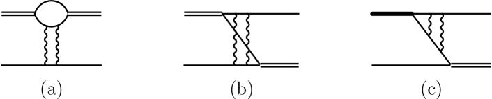
Figure 2: Two-photon three-nucleon diagrams. Solid lines represent nucleons whereas a deuteron (${}^{1}S_{0}$ dibaryon) is drawn as a double (thick) line. Wavy lines are Coulomb photons.

Figure 3: Two-photon bubble. Symbols are as in Fig. 2.

The basic ingredient for all these topologies is the two-photon loop diagram shown in Fig. 4. This could be calculated directly, but it is more convenient to simply extract it as the $\mathcal{O}(\alpha^{2})$ piece of the full off-shell Coulomb T-matrix.

Figure 4: General two-photon exchange diagram. Symbols are as in Fig. 2.

For general kinematics with incoming (outgoing) momentum $\mathbf{p}$ ($\mathbf{q}$) and center-of-mass energy $E=k^{2}M_{N}$, this T-matrix can be written in the Hostler form Chen:1972ab; Hostler:1964aa; Hostler:1964ab

$$T_{C}(k;\mathbf{p},\mathbf{q})=\frac{\!4\pi\alpha}{(\mathbf{p}-\mathbf{q})^{2}}\left\{1-2\mathrm{i}\eta\int_{1}^{\infty}\left(\frac{s+1}{s-1}\right)^{\!\!-\mathrm{i}\eta}\frac{\mathrm{d}s}{s^{2}-1-\epsilon}\right\}\ \ \text{,}\ \ \epsilon=\frac{(p^{2}-k^{2})(q^{2}-k^{2})}{k^{2}(\mathbf{p}-\mathbf{q})^{2}}\,,$$ (26)

where

$$\eta(k)=\frac{\alpha M_{N}}{2k}$$ (27)

This form is most suitable for extracting the two-photon piece because it is straightforward to expand in $\alpha$. Noting that $\eta=\mathcal{O}(\alpha)$ gives

$$T_{C}^{(2)}(k;\mathbf{p},\mathbf{q})=({-}2\mathrm{i}\eta)\frac{4\pi\alpha}{(\mathbf{p}-\mathbf{q})^{2}}\int_{1}^{\infty}\frac{\mathrm{d}s}{s^{2}-1-\epsilon}={-}\mathrm{i}\frac{4\pi\alpha^{2}M_{N}}{k(\mathbf{p}-\mathbf{q})^{2}}\frac{\mathrm{atanh}\left(\sqrt{1+\epsilon}\right)}{\sqrt{1+\epsilon}}\,.$$ (28)

A numerical comparison with the bare expression obtained from Fig. 4—which involves a brute-force three-dimensional momentum integration—gives excellent agreement with Eq. (28).

The diagrams shown in Fig. 2 can now be expressed in terms of $T_{C}^{(2)}$, based on previous results including the full Coulomb T-matrix Konig:2014ufa (cf. also Refs. Kok:1979aa; Kok:1981aa; Ando:2010wq). Explicit expressions are given in Appendix LABEL:sec:CoulombKernels.

Only the diagram with two photons exchange inside a bubble, shown in Fig. 3, requires some further work. In principle, it can be obtained by integrating $T_{C}^{(2)}(k;\mathbf{p},\mathbf{q})$ over $\mathbf{p}$ and $\mathbf{q}$, but that would be unnecessarily tedious. More conveniently, it can be extracted from the full Coulomb Green’s function Hostler:1963zz; Meixner:1933aa,

$$G_{C}(E;\mathbf{r}^{\prime}=\mathbf{0},\mathbf{r})={-}2\mu\frac{\Gamma(1-\mathrm{i}\eta)\,W_{\mathrm{i}\eta;1/2}(-2\mathrm{i}kr)}{4\pi r}\ \ \text{,}\ \ \eta=\frac{\alpha\mu}{k}\ \ \text{,}\ \ \mu=\frac{M_{N}}{2}\,.$$ (29)

in the limit $\mathbf{r}\to 0$. When this is expanded in $\alpha$, the first to terms are divergent, but the $\mathcal{O}(\alpha^{2})$ and all higher orders are finite Kong:1999sf; Kong:2000px. Expanding Eq. (29) first in $r$ and subsequently in $\alpha$ gives

$$\frac{1}{2\mu}G_{C}(E;\mathbf{r}^{\prime}=\mathbf{0},\mathbf{r})=\text{div.\ terms}-\frac{\mathrm{i}k}{4\pi}+\frac{\alpha\mu\big{[}\log({-}2\mathrm{i}k)+C_{E}-1\big{]}}{2\pi}-\frac{\mathrm{i}\mu^{2}\pi\alpha^{2}}{12k}+\mathcal{O}(r,\alpha^{3})\,,$$ (30)

such that one can read off

$$\delta J_{0}^{(2)}(k)={-}\frac{M_{N}}{4\pi}\left[\frac{\mathrm{i}\pi^{2}\alpha^{2}M_{N}^{2}}{12k}\right]\,.$$ (31)

The label $\delta J_{0}^{(2)}(k)$ was chosen because alternatively this piece can be extracted from the Coulomb bubble summing up two and more photon exchanges, which Ref. Konig:2015aka showed to be

$$\delta J_{0}(k)={-}\frac{\alpha M_{N}^{2}}{4\pi}\left[\psi(\mathrm{i}\eta)+\frac{1}{2\mathrm{i}\eta}+C_{\Delta}\right]+\frac{M_{N}}{4\pi}\mathrm{i}k\,.$$ (32)

Expanding the digamma function as

$$\psi(x)={-}\frac{1}{x}-C_{E}+\frac{\pi^{2}x}{6}+\mathcal{O}(x^{2})$$ (33)

gives again Eq. (32) and provides a consistency check. In fact, all higher-order Coulomb contributions can be obtained in the same way as described here.

II.5 Propagator corrections

Next-to-leading order corrections to the dibaryon propagators are have been discussed in great detail in Ref. Konig:2015aka. They are exactly the same here for the expansion that only takes the ${}^{1}S_{0}$ channel in the unitarity leading order. For the “full unitarity” expansion introduced in Ref. Konig:2016utl, the ${}^{3}S_{1}$ channel is taken in the same limit at LO, such that generically [eq:Delta-dt-0-1] iΔ_d,t^(0)(p_0,p) &= -iσd,t(0)+ yd,t2I0(p0,p)
iΔ_t^(1)(p_0,p) = iΔ_d,t^(0)(p_0,p)×[-iσ_d,t^(1) - ic_d,t^(1) (p_0-p24MN) ] ×iΔ_d,t^(0)(p_0,p)  . with

$$\sigma_{d,t}^{(0)}=\frac{2\Lambda}{\pi}\ \ \text{,}\ \ \sigma_{d,t}^{(1)}={-}\frac{1}{a_{d,t}}\ \ \text{,}\ \ c_{d,t}^{(1)}=\frac{M_{N}r_{d,t}}{2}\,.$$ (34)

In particular, while in the standard and ${}^{1}S_{0}$-unitarity LO the ${}^{3}S_{1}$ propagator is matched to the effective range expansion around the deuteron pole, giving

$$\sigma_{d}^{(1)}=\frac{\rho_{d}\gamma_{d}^{2}}{2}\ \ \text{,}\ \ c_{d}^{(1)}=\frac{M_{N}\rho_{d}}{2}\,,$$ (35)

the ordinary expansion around zero energy is used in the full-unitarity case to treat both channels fully equivalently. Either way, at N${}^{2}$LO there are quadratic insertions of $\sigma_{d,t}^{(1)}$ and $c_{d,t}^{(1)}$,

$$\mathrm{i}\Delta_{t}^{(2)}(p_{0},\mathbf{p})=\mathrm{i}\Delta_{t}^{(0)}(p_{0},\mathbf{p})\times\Bigg{\{}\bigg{[}{-}\mathrm{i}\sigma_{t}^{(1)}-\mathrm{i}c_{d,t}^{(1)}\left(p_{0}-\frac{\mathbf{p}^{2}}{4M_{N}}\right)\Bigg{\}}^{\!2}\,,$$ (36)

and of course this matches directly onto the expansion of the renormalized amplitude when the expressions from Eq. (34) are inserted. Note that the generic dibaryon parameter $\sigma$ (in a given channel) is related the corresponding “ordinary” $C_{0}$ used in Sec. II.3 via $\sigma={-}{4\pi}/{(M_{N}C_{0})}$. This means that their formal expansions are different, and in general, for a fixed scattering length included at NLO, one has $\sigma_{t(,pp)}^{(n)}=0$ for $n\geq 2$. In the $nd$ sector, however, there is a correction $\sigma_{t,nn}^{(2)}={-}1/a_{t,nn}+1/a_{t}$ which shifts the inverse scattering length away from its isospin-symmetric value.

In the $pp$ channel, there are Coulomb contributions as well. Most notably, the bubble with a single photon exchanged inside—denoted as $\delta I_{0}(k)$— is logarithmically divergent, and this divergence is absorbed by setting Konig:2015aka

$$\sigma_{t,pp}^{(1)}={-}\frac{1}{a_{C}}-\alpha M_{N}\left(\log\dfrac{2\Lambda}{\alpha M_{N}}-C_{\zeta}-C_{\Delta}\right)$$ (37)

with known constants $C_{\zeta}$ and $C_{\Delta}$. NLO also includes isospin-symmetric range corrections given by $c_{t}^{(1)}$. At N${}^{2}$LO, there are quadratic insertions of $\sigma_{t,pp}^{(1)}$, $c_{t}^{(1)}$, and $\delta I_{0}(k)$, but in addition also the isospin-breaking range correction $c_{t,pp}^{(2)}=M_{N}(r_{C}-r_{t})/2$ and the genuine two-photon contribution $\delta J_{0}^{(2)}(k)$ discussed in the previous section. Overall, this amounts to iΔ_t,pp^(2)(p_0,p) &= iΔ_t,pp^(0)(p_0,p)×{[-iσ_t,pp^(1) - ic_t^(1) (p_0-p24MN)
                           - iy_t^2δI_0​(ip^2/4-M_Np_0-iε)] ×iΔ_t,pp^(0)(p_0,p)}^​2
+ iΔ_t,pp^(0)(p_0,p)×[ -ic_t,pp^(2) (p_0-p24MN)
                           - iy_t^2δJ_0^(2)​(ip^2/4-M_Np_0-iε) ]×iΔ_t,pp^(0)(p_0,p)  , and inserting the various definitions this simplifies to iΔ_t,pp^(2)(p_0,p) &= -i{1aC- αMN[CΔ+ log​(αMN2~k(p0,p))]+ rt2~k(p0,p)2}​2- π2α2MN212~k(p0,p)3
- irC- rt2  , where $\tilde{k}(p_{0},\mathbf{p})\equiv\sqrt{{\mathbf{p}^{2}}/{4}-M_{N}p_{0}-\mathrm{i}\varepsilon}$.

III Three-body observables up to N${}^{2}$LO

III.1 Integral equations

Adapting the notation of Refs. Konig:2014ufa; Konig:2015aka, the LO amplitude is a three-vector in channel space (with the last two components corresponding to $np$ and $pp/nn$ singlet-dibaryon legs):

$$\vec{\mathcal{T}}_{\mathrm{s}}\equiv\left(\mathcal{T}_{\mathrm{s}}^{\mathrm{d,a}},\mathcal{T}_{\mathrm{s}}^{\mathrm{d,b1}},\mathcal{T}_{\mathrm{s}}^{\mathrm{d,b2}}\right)^{T}\,.$$ (38)

It is determined by the integral equation

$$\vec{\mathcal{T}}_{\mathrm{s}}^{(0)}={-}\hat{K}^{(0)}\vec{e}_{1}+(\hat{K}^{(0)}\hat{D}^{(0)})\otimes\vec{\mathcal{T}}_{\mathrm{s}}^{(0)}\,,$$ (39)

where $\vec{e}_{1}=(1,0,0)^{T}$ and $\otimes$ represents an integral over the intermediate momentum,

$$A\otimes B\equiv\frac{1}{2\pi^{2}}\int_{0}^{\Lambda}\mathrm{d}q\,q^{2}\,A(\ldots,q)B(q,\ldots)\,,$$ (40)

involving a momentum cutoff $\Lambda$. $\hat{D}^{(0)})$ is a diagonal matrix of dibaryon propagators, viz.

$$\hat{D}^{(n)}=\mathrm{diag}\left(D_{d}^{(n)},D_{t}^{(n)},D_{t(,pp)}^{(n)}\right)\,,$$ (41)

where generically $D_{x}^{(n)}(E;q)\equiv\Delta_{x}^{(n)}\big{(}E-q^{2}/(2M_{N});q\big{)}$, and the kernel matrix is

$$\hat{K}^{(0)}=2\pi\begin{pmatrix}{-}\left(K_{\mathrm{s}}+\frac{2H_{0,0}(\Lambda)}{\Lambda^{2}}\right)&\left(3K_{\mathrm{s}}+\frac{2H_{0,0}(\Lambda)}{\Lambda^{2}}\right)&\left(3K_{\mathrm{s}}+\frac{2H_{0,0}(\Lambda)}{\Lambda^{2}}\right)\\[5.0pt] \left(K_{\mathrm{s}}+\frac{2H_{0,0}(\Lambda)}{3\Lambda^{2}}\right)&\left(K_{\mathrm{s}}-\frac{2H_{0,0}(\Lambda)}{3\Lambda^{2}}\right)&{-}\left(K_{\mathrm{s}}+\frac{2H_{0,0}(\Lambda)}{3\Lambda^{2}}\right)\\[5.0pt] \left(2K_{\mathrm{s}}+\frac{4H_{0,0}(\Lambda)}{3\Lambda^{2}}\right)&{-}\left(2K_{\mathrm{s}}+\frac{4H_{0,0}(\Lambda)}{3\Lambda^{2}}\right)&{-}\frac{4H_{0,0}(\Lambda)}{3\Lambda^{2}}\end{pmatrix}\,.$$ (42)

It describes the isospin-symmetric system without Coulomb contributions and thus only contains the one-nucleon exchange part $K_{\mathrm{s}}$ and the LO three-nucleon force $H_{0,0}$. For more detailed definitions, see Ref. Konig:2014ufa.

As indicated by the subscript “$\mathrm{s}$,” the LO equation only contains contributions from the strong interaction. The additional inclusion of Coulomb effects perturbatively builds up the “full” amplitude. Up to N${}^{2}$LO, the corresponding integral equations are

$$\vec{\mathcal{T}}_{\mathrm{full}}^{(1)}={-}\hat{K}^{(1)}\vec{e}_{1}+\left[\hat{K}^{(1)}\hat{D}^{(0)}+\hat{K}^{(0)}\hat{D}^{(1)}\right]\otimes\vec{\mathcal{T}}_{\mathrm{full}}^{(0)}+(\hat{K}^{(0)}\hat{D}^{(0)})\otimes\vec{\mathcal{T}}_{\mathrm{full}}^{(1)}$$ (43)

and

$$\vec{\mathcal{T}}_{\mathrm{full}}^{(2)}={-}\hat{K}^{(2)}\vec{e}_{1}+\left[\hat{K}^{(2)}\hat{D}^{(0)}+\hat{K}^{(1)}\hat{D}^{(1)}+\hat{K}^{(0)}\hat{D}^{(2)}\right]\otimes\vec{\mathcal{T}}_{\mathrm{full}}^{(0)}\\ +\left[\hat{K}^{(1)}\hat{D}^{(0)}+\hat{K}^{(0)}\hat{D}^{(1)}\right]\otimes\vec{\mathcal{T}}_{\mathrm{full}}^{(1)}+(\hat{K}^{(0)}\hat{D}^{(0)})\otimes\vec{\mathcal{T}}_{\mathrm{full}}^{(2)}\,,$$ (44)

with $\vec{\mathcal{T}}_{\mathrm{full}}^{(0)}=\vec{\mathcal{T}_{\mathrm{s}}}^{(0)}$. Essentially, the structure is the same as in the two-body example discussed in Sec. II.3, only that here there are two types of corrections:

1. Contributions to the dibaryon propagators (from finite scattering lengths and effective ranges as well as two-body Coulomb effects in the $pp$ subsystem), encoded in the general expression given in Eq. (41).

2. The associated three-body force corrections as well as three-body Coulomb diagrams contributing to the higher-order interaction-kernel matrices.

Specifically, these matrices are

$$\hat{K}^{(1)}=2\pi\begin{pmatrix}{-}\left(K_{\text{bub}}+K_{\text{box}}+\frac{2H_{0,1}(\Lambda)}{\Lambda^{2}}\right)&\left(3K_{\text{box}}+\frac{2H_{0,1}(\Lambda)}{\Lambda^{2}}\right)&\left(3K_{\text{tri}}^{(\text{out})}+\frac{2H_{0,1}(\Lambda)}{\Lambda^{2}}\right)\\[5.0pt] \left(K_{\text{box}}+\frac{2H_{0,1}(\Lambda)}{3\Lambda^{2}}\right)&{-}\left(K_{\text{bub}}-K_{\text{box}}+\frac{2H_{0,1}(\Lambda)}{3\Lambda^{2}}\right)&{-}\left(K_{\text{tri}}^{(\text{out})}+\frac{2H_{0,1}(\Lambda)}{3\Lambda^{2}}\right)\\[5.0pt] \left(2K_{\text{tri}}^{(\text{in})}+\frac{4H_{0,1}(\Lambda)}{3\Lambda^{2}}\right)&{-}\left(2K_{\text{tri}}^{(\text{in})}+\frac{4H_{0,1}(\Lambda)}{3\Lambda^{2}}\right)&{-}\frac{4H_{0,1}(\Lambda)}{3\Lambda^{2}}\end{pmatrix}$$ (45)

and

$$\hat{K}^{(2)}=2\pi\begin{pmatrix}{-}\left(K_{\text{bub}}^{(2)}+K_{\text{box}}^{(2)}+2H^{(2)}\right)&\left(3K_{\text{box}}+2H^{(2)}\right)&\left(3K_{\text{tri}}^{(\text{2,out})}+2H^{(2)}\right)\\[5.0pt] \left(K_{\text{box}}^{(2)}+\frac{2}{3}H^{(2)}\right)&{-}\left(K_{\text{bub}}^{(2)}-K_{\text{box}}^{(2)}+\frac{2}{3}H^{(2)}\right)&{-}\left(K_{\text{tri}}^{(\text{2,out})}+\frac{2}{3}H^{(2)}\right)\\[5.0pt] \left(2K_{\text{tri}}^{(\text{2,in})}+\frac{4}{3}H^{(2)}\right)&{-}\left(2K_{\text{tri}}^{(\text{2,in})}+\frac{4}{3}H^{(2)}\right)&{-}\frac{4}{3}H^{(2)}\end{pmatrix}\\ \hbox{}+2\pi\,\mathrm{diag}\big{(}K_{\rho_{d}},K_{r_{t}},0\big{)}\,,$$ (46)

where the collection of N${}^{2}$LO three-nucleon forces is

$$H^{(2)}(\Lambda)=\frac{H_{0,2}(\Lambda)}{\Lambda^{2}}+\frac{H_{2,2}(\Lambda)}{\Lambda^{4}}(M_{N}E+\gamma_{d}^{2})+\frac{H_{0,2}^{(\alpha)}(\Lambda)}{\Lambda^{2}}\,.$$ (47)

The functions $K_{\text{bub}}^{(2)}$, $K_{\text{box}}^{(2)}$, and $K_{\text{tri}}^{(\text{2,out})}$ correspond, respectively, to the three diagrams shown in Fig. 2. $K_{\text{tri}}^{(\text{2,in})}$ comes from the reversed version of Fig. 2(c), where the photon exchanges are on the left side of the diagram. Detailed expressions for all these functions are given in the Appendix LABEL:sec:CoulombKernels. The analogous one-photon functions in Eq. (45) are defined (for example) in Ref. Konig:2015aka and are thus not repeated here. Finally, the contributions $K_{\rho_{d}}$ and $K_{r_{t}}$, corresponding to a direct coupling of photons to the dibaryons,

$$K_{r}(E;k,p)={-}\frac{\alpha M_{N}r}{2kp}\,Q_{0}\!\left(-\frac{k^{2}+p^{2}+\lambda^{2}}{2kp}\right)\ \ \text{,}\ \ Q_{0}(x)=\frac{1}{2}\log\left(\frac{x+1}{x-1}\right)\ \ \text{,}\ \ r=\rho_{d},r_{t}\,,$$ (48)

enter at N${}^{2}$LO in the power counting ($\lambda$ here is a small photon mass introduced as infrared regulator and discussed further in the next section).

Note that the new three-body force $H_{0,2}^{(\alpha)}(\Lambda)$ is needed due to terms mixing range corrections and $O(\alpha)$ Coulomb contributions. While from the N${}^{2}$LO calculation based on the T-matrix method it is not directly obvious, one can identify contributions to the energy shift of the form

$$\parbox{53.19963pt}{\hbox{\raisebox{1.99997pt}{\includegraphics[width=50.00008pt]{DeltaE-bubble-rd}} }}\sim\;\left(\frac{1}{q}\right)^{\!2}_{\!\!\mathcal{B}}\times\Big{(}q^{3}\Big{)}^{3}_{\!\text{loops}}\times\left(\frac{1}{q^{2}}\right)^{\!2}_{\!\!N}\times\left(\frac{1}{q}\right)^{\!3}_{\!\!D}\times\left(\frac{1}{q^{2}}\right)_{\!\text{photon}}\times\Big{(}q^{2}\Big{)}_{\!\text{range corr.}}\;\sim\;q^{0}\,,$$ (49)

where all loop momenta have been generically denoted by $q$ and the notation of Ref. Konig:2014ufa has been adapted to count ultraviolet behavior diagram. This, as well as similar diagrams involving other topologies and/or a direct dibaryon-photon coupling, are logarithmically divergent, such that the three-body forces determined from the $nd$ system alone are no longer sufficient to ensure renormalization.

III.2 Extraction of binding energies

Binding energies can be obtained by plugging the solutions of the integral equations into the expressions given in Sec. II.2. At LO, this merely amounts to varying the energy until the homogeneous version of Eq. (39) has a solution. When the LO three-nucleon force is fitted to the physical triton binding energy, the energy is fixed at that value and $H_{0,0}(\Lambda)$ is varied (for a given value of $\Lambda$).

The perturbative corrections to the binding energy are defined in terms of limits where the energy approaches the LO pole. Numerically, this is evaluated by varying the energy around the pole and interpolating with a low-order polynomial to extract the residues (a linear interpolation is found to be sufficient in most cases if a 1% interval around the pole is considered). The reliability of this procedure has been checked by comparing NLO results with those obtained as matrix elements between leading-order vertex functions (as described, for example, in Ref. Konig:2015aka), finding excellent agreement.

III.3 Subtracted phase shifts

For $pd$ scattering it is necessary to calculate Coulomb-subtracted phase shifts $\tilde{\delta}(k)\equiv\delta_{\mathrm{full}}(k)-\delta_{\mathrm{c}}(k)$, where the first term—corresponding to the combination of strong and Coulomb contributions—is extracted perturbatively from the full amplitude (specifically, from the the $pd\to pd$ component $\mathcal{T}_{\mathrm{full}}\equiv\mathcal{T}_{\mathrm{full}}^{\mathrm{d,a}}$). Up to N${}^{2}$LO, the expressions are δ_full^(0)(k) &= 12i log​(1+ikμπ T_full^(0)(k))  ,
δ_full^(1)(k) = kμ2π Tfull(1)(k)1+ikμπTfull(0)(k)  ,
δ_full^(2)(k) =