A Smolin-like branching multiverse from multiscalar-tensor theory

Abstract

We implement a Smolin-like branching multiverse through a directed, acyclic graph of $N$ metrics. Our gravitational and matter actions are indistinguishable from $N$ decoupled statements of General Relativity, if one varies with respect to metric degrees of freedom. We replace $N-1$ metrics with scalar fields by conformally relating each metric to its unique graph predecessor. Varying with respect to the $N-1$ scalar fields gives a multiscalar-tensor model which naturally features dark matter candidates. Building atop an argument of Chapline and Laughlin, branching is accomplished with the emergence of order parameters during gravitational collapse: we bootstrap a suitably defined $N$ scalar field model with initial data from an $N-1$ field model. We focus on the nearest-neighbour approximation, determine conditions for dynamical stability, and compute the equations of motion. The model features a novel screening property where the scalar fields actively adjust to decouple themselves from the stress, oscillating about the requisite values. In the Newtonian limit, these background values for the scalar fields exactly reproduce Newton’s law of gravitation.

I Introduction

In 1992, Lee Smolin posed the questionSmolin (1992), “Did the Universe Evolve?” His use of the word “evolve” was not in the physicists’ sense of dynamical time evolution, but in the biologists’ sense of speciation. Smolin proposed that gravitational collapse produces an offspring Universe with slightly different Standard Model (SM) parameters from the progenitor: a microphysical analogy to the microbiology of inheritance. After many generations, he argued, we should find ourselves at a local maximum over SM parameter space for the formation of collapsed objects. In this way, he proposed a fascinating resolution to the Hierarchy Problem: it is our notion of naturalness that we must adjust.

Of the criticisms (e.g. Smolin (2006)) levelled against Smolin’s 1992 proposal, the only one relevant is that it disagrees with observation (e.g. Rothman and Ellis (1993)). We regard this result as refutation only of Smolin’s particular fitness function: reproductive rate. Note that this fitness function is appropriate in the simplest of scenarios: e.g. bacteria with unlimited food. In any realistic setting, one cannot consider the organism in isolation; competition and environmental pressures ultimately determine the fate of populations. In fact, it is observation of how interacting organisms within populations change over timescales much greater than an individual’s lifespan which led to Darwin’s conclusionsDarwin (1872) on fitness, not the other way around.

The purpose of this paper is to develop a notion of population and ancestry via an extension to the Einstein-Hilbert action. We restrict ourselves to SM clones for simplicity, as we have yet no experimental basis for speculation on the microphysical origins of speciation. Our approach combines two well-motivated lines of extension to General Relativity (GR): multiscalar-tensor theories and multiple metric theories. There is a vast and mature literature on scalar-tensor theories. Not only have their observational signatures been rigorously characterised(e.g. Damour and Esposito-Farese (1992, 1993)), but scalar fields are well known to contribute negative pressure, and are a mainstay of primordial inflation scenariosBassett et al. (2006). Multiple metric theories also have a long history (e.g. Rosen (1963)), with well-known pathologiesWill (1993); Boulanger et al. (2001) having motivated novel and potentially viable (e.g. Hassan and Rosen (2012)) approaches. The result of our effort will be a classical field theory which makes quantitative predictions amenable to immediate confrontation with existing and future astrophysical data.

The rest of this paper is organised as follows. We first review the necessary technical background and emphasise some common caveats when working in multiple metric settings. We then motivate and introduce our gravitational and matter actions, featuring $N$ metric degrees of freedom. Through conformal relations, we establish a consistent notion of causality across the $N$ metrics by replacing $N-1$ metric degrees of freedom with scalar degrees of freedom. We perturbatively expand the resulting gravitational action, which takes the form of a multiscalar-tensor theory in the Jordan frame, and determine conditions for dynamical stability. We compute the equations of motion, demonstrate the consistency of our branching process, and examine the Newtonian limit. We then discuss very many future directions and conclude. An appendix presents a conceptually related model as a foil to emphasise our particular approach. A second appendix outlines an alternate route to a model with many of the features developed in the main body, with differing aesthetic criteria that may appeal to some researchers. Throughout the paper, we employ units where $c\equiv 1$. Note that we will define notation at its introduction, and will often abbreviate “stress-energy” as simply “stress.” If context should require distinction, it will be made explicitly.

II The phylogenic model

We briefly review some of the mathematics involved when considering multiple metrics defined on a common differentiable manifold $\mathscr{M}$ of dimension $n$. First recall any suitable almost everywhere $C^{\infty}$ differentiable manifold admits the notion of curves independently of any geometry. These objects are maps $C(\tau):\mathscr{M}\leftarrow\tau\in[a,b]\subset\mathbb{R}$ which, when composed with the coordinate charts $\xi^{i}:\mathbb{R}\leftarrow\mathscr{M}$, become real-valued differentiable functions $\xi^{i}\circ C$. Derivatives of these compositions can then be used, in a natural wayO’neill (1983), to construct tangent and cotangent spaces on $\mathscr{M}$.

At one’s discretion, notions like metric, connection, and volume form (Jacobian) can be introduced to augment $\mathscr{M}$. There is no natural notion of uniqueness for any of these objects. Given a metric, however, one may uniquely construct a torsion-free connection compatible with this metric. This Levi-Civita connection is the only type which we consider below.

Observers using distinct metrics will arrive at distinct physical conclusions. For example, fix two events $x^{\mu}$ and ${x^{\prime}}^{\mu}$ on $\mathscr{M}$ and fix some curve $C$ such that $C(\tau_{i})\equiv x^{\mu}$ and $C(\tau_{f})\equiv{x^{\prime}}^{\mu}$. As stated above, this curve has a field of velocity vectors $\mathrm{d}C^{\mu}/\mathrm{d}\tau$ that exist independently of any geometry. If $C$ is always time-like with respect to metrics labelled $p$ and $q$, then we may consider the proper separation as perceived by observers using metric $p$ versus observers using metric $q$. It may happen that

$$\int_{C}\sqrt{\overset{p}{g}_{\mu\nu}\frac{\mathrm{d}x^{\mu}}{\mathrm{d}\tau}\frac{\mathrm{d}x^{\nu}}{\mathrm{d}\tau}}~{}\mathrm{d}\tau\neq\int_{C}\sqrt{\overset{q}{g}_{\mu\nu}\frac{\mathrm{d}x^{\mu}}{\mathrm{d}\tau}\frac{\mathrm{d}x^{\nu}}{\mathrm{d}\tau}}~{}\mathrm{d}\tau.$$ (1)

Physically, the presence of multiple metrics requires an additional means of assigning “measurement apparatus” to observers, and this assignment partitions observers into distinct classes. For clarity, “observers” continues to mean “frames which arrive at the same physical conclusions under diffeomorphism.” We regard this property as a virtue of multiple metric theories, in that such theories simultaneously acknowledge the mathematical non-uniqueness of metric and remove the unique class of observers from GR. This uniqueness in GR infamously led to Fock’s somewhat amusing complaint of, “a widespread misinterpretation of the Einsteinian Gravitation Theory as some kind of general relativity.”Fock (2015).

In the multimetric setting, care must be exercised when executing common tensor operations. Raising and lowering indices on an $q$-labelled object can only be accomplished with the $q$ metric. For example

$$\overset{q}{R_{\mu\nu}}\overset{p}{g^{\mu\rho}}\neq\overset{q}{R^{\rho}}_{\nu}$$ (2)

and cannot be simplified further, without additional information relating the $p$-metric to the $q$-metric. Likewise there are now distinct covariant derivatives, which are only compatible with their paired metrics. In other words

$$\overset{p}{\nabla}_{\mu}\left(\overset{q}{g^{\mu\nu}}\overset{p}{T_{\nu\rho}}\right)\neq\overset{q}{g^{\mu\nu}}\overset{p}{\nabla}_{\mu}\overset{p}{T_{\nu\rho}}$$ (3)

because the $q$ metric is not compatible with the $p$ connection and so cannot be commuted through this covariant differentiation.

II.1 The phylogenic matter and gravitational actions

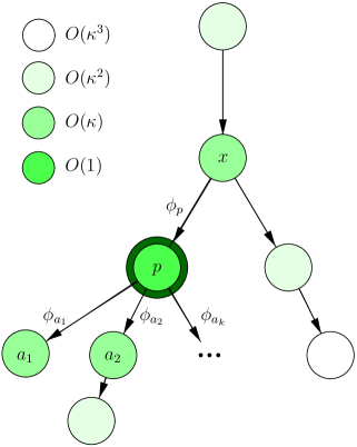
Figure 1: Directed, acyclic graph representation of couplings, conformal relations, and relative orders for a model anchored at $p$. Note terms $O(\kappa^{2})$ are discarded in the nearest-neighbour model of §III.

The utility of GR and its metric foundation, as a quantitative model for reality, has been rigorously verified over many decades of spatiotemporal scale. Consequently, any departures from GR must either be very slight, subtly hidden, or both. Consider a population of $N$ metrics and $N$ copies of the SM. Introduce a dimensionless coupling constant $\kappa>0$, and consider a directed, acyclic graph (DAG) e.g. the rooted tree of Figure 1. Associate to each vertex $q$ of this tree a distinct metric $g^{q}_{\mu\nu}$ and stress $T^{q}_{\mu\nu}$. Given any two vertices $p$ and $q$ of this graph, let $r(p,q)\geq 0$ be the graph distance between vertex $p$ and vertex $q$. This distance is well-defined because there is a unique simple path between any two vertices of a tree. We assign observers to metrics by augmenting a straightforward generalisation of the canonical matter action, due to Hohmann and WohlfarthHohmann and Wohlfarth (2010), with the graph distance between $p$ and $q$

$$\delta\overset{p}{S}_{M}\equiv-{1\over 2}\int\mathrm{d}^{4}\xi~{}\sum_{q}^{N}\kappa^{r(p,q)}\overset{q}{T}_{\mu\nu}\delta\overset{q}{g^{\mu\nu}}\sqrt{q}.$$ (4)

Here $\sqrt{q}$ is shorthand for the natural volume form induced by the $q$ metric. Note that these $N$ matter actions, indexed by $p$, each enforceFock (2015) $N$ distinct statements of the Equivalence Principle: observers using the $q$ metric will observe $q$ stress to follow $q$ metric geodesics.

Multiple metric gravitational actions are tightly constrained. With the exception of Hassan and Rosen’s multiple metric theoryHassan and Rosen (2012), Theorem 1.1 of Boulanger et. al. Boulanger et al. (2001) demands that all metrics must be decoupled. We thus consider the class of models indexed by $p$

$$\overset{p}{S}_{G}\equiv\frac{1}{16\pi G}\int\mathrm{d}^{4}\xi~{}\sum_{q}^{N}\kappa^{r(p,q)}\overset{q}{R}\sqrt{q}$$ (5)

where powers of $\kappa$ enter in the same manner as (4). Note that these actions suggest a natural perturbative treatment in powers of $\kappa$. If one varies the gravitational actions (5) with respect to the metric degrees of freedom, combination with (4) recovers $N$ distinct statements of exactly Einstein’s equations for each $q$. Thus, there is no way to experimentally distinguish any of these actions from that of Hilbert and we have successfully hidden our new degrees of freedom.

II.2 Conformal relations and ancestry

An undesirable feature of any model with $N$ possibly distinct metrics is $N$ distinct notions of causal ordering. We resolve this issue, introduce coupling, and bring the model very close to already well-established literature by demanding that each vertex’s metric be conformally related to its unique graph parent. Let $p$ have a set of children $\{a_{1},\dots,a_{n_{a}}\}$. Then, for the $i$-th child, there exists a scalar field $\phi_{a_{i}}$ and constants $\sigma_{a_{i}}$ such that

$$\overset{a_{i}}{g}_{\mu\nu}\equiv\exp(\sigma_{a_{i}}\phi_{a_{i}})\overset{p}{g}_{\mu\nu}$$ (6)

where we have used the standard exponential parameterisation with the factor of two removed for economy of notation. Note that, from any child’s perspective, the parent metric acquires an inverted sign

$$\overset{p}{g}_{\mu\nu}=\exp(-\sigma_{a_{i}}\phi_{a_{i}})\overset{a_{i}}{g}_{\mu\nu}.$$ (7)

These $N-1$ scalar fields define the edges of the graph and replace $N-1$ metric degrees of freedom.

Note carefully that the model is no longer permutation symmetric. In other words, for distinct $p$, the resultant models from application of the extrema principle will yield non-equivalent equations of motion. Nevertheless, the qualitative behaviour observed in all such models will be unchanged. This can be seen by considering a model where each vertex has a fixed number of children $n_{a}$ and the tree is countably infinite. In this limit, one would have perfect permutation symmetry. For a discussion of an absolutely permutation invariant construction, and why we have avoided this model, we refer the interested reader to Appendix §A. In the remainder of our discussion, we will focus on a specific model anchored at $p$. We will use the word “native” to refer to tensors associated with vertex $p$, and the word “foreign” to refer to tensors associated with other vertices. Special attention must be paid to the scalar fields, however, as they define the graph’s edges, and are a property defined between two vertices.

II.3 Asexual reproduction and scalar potentials

Our next task is to implement the Smolin-like branching process, which he assumes to be associated with black hole (BH) production. The approach we will take is distinctly pragmatic, and motivated from condensed matter systems. Consider the bulk magnetisation of a ferromagnetic material as it passes through the Curie Temperature from above. Here, a vector degree of freedom enters the dynamics at a phase transition. In complete analogy, we assume that a scalar degree of freedom $\phi_{a}$ and a tensor degree of freedom $T^{a}_{\mu\nu}$ enter the dynamics during gravitational collapse. In this way, we seek to implement a proposal of Chapline and Laughlin who, a decade earlier, arguedChapline (2003); Chapline et al. (2001) that one really should replace the singular collapse scenario with a phase transition. We will glue an $N$ vertex model to a separate $N+1$ vertex model, both anchored at $p$, using the final data of the $N$-vertex model fields to “bootstrap” the initial data of the $N+1$ model in a consistent fashion.

Chapline and Laughlin assert that the simplest scenario resulting from their phase transition should be an interior GR vacuum solution with anomalously large cosmological constant. Adapted to our context, in its simplest form, this can be accomplished by a single scalar field dominated by potential. Yet unlike the matter actions, which are constrained by the Equivalence Principle; and the gravitational actions, which are constrained by Boulanger, et. al.; in the absence of a comprehensive theory, a potential is explicitly phenomenological. There is an extremely rich literature on inflationary potentials, their observational signatures, and their use in resolving outstanding problems in particle physics (for an excellent review, see Bassett et al. (2006)). Inflationary theory, however, is dominated by particle and quantum-field theoretic concepts, and any foray would be premature given the present limited scope. Thus, we only partially constrain the specific form of $V$, and instead focus on how potentials should enter our actions.

Using Rosen’s notationRosen and Krithivasan (1995), let $[A_{qw}]$ be the adjacency matrix for the ancestral tree. Let $d(p,q)$ be the signed relative graph depth (c.f. $r(p,q)$) between vertex $p$ and vertex $q$, with ancestors negative consistent with (7). We define

$$\overset{p}{S}_{V}\equiv-\frac{1}{8\pi G}\int\mathrm{d}^{4}\xi~{}\sum_{q}^{N}\sum_{w>q}\kappa^{r(p,w)}[A_{qw}]V(\phi_{w})\sqrt{w}$$ (8)

where the notation $w>q$ means to consider pairings such that $w$ satisfies $d(p,w)>d(p,q)$. Note that $V:\mathcal{F}(\mathscr{M})\leftarrow\mathcal{F}(\mathscr{M})$ is a fixed map understood to have dimension of inverse length squared. A single map is consistent with the Copernican Principle and our restriction to a population of SM clones. In reheating scenarios, energy within the scalar field is transferred to SM degrees of freedom. The Equivalence Principle then suggests an absence of cross-couplings between scalar fields in $V$. Note again that, assuming no active scalar degrees of freedom, one just regenerates $N$ distinct cosmological constants.

II.4 A possible observational signature

An interesting and immediate consequence of (6) is that all members of the ancestral tree share the same (tensor) gravitational radiation field in vacuum. This is because the conformally invariant Weyl tensor is the only non-zero component of the Riemann tensor in vacuum. This is consistent with the presence of a single metric degree of freedom, whose quantized linearization would supposedly provide the graviton. Since the radiation field is shared, a significantly higher than expected observation rate for BH mergers (e.g. Abbott et al. (2016)) could be the result of foreign sources. Given sufficient directionality, at distances near enough to the Earth for appreciable amplitude, a slightly aspherical supernova gravitational wave signature coupled with a lack of observation in the EM and neutrino sectors would be a “smoking gun” independent of gravitational wave polarisation.

III The nearest-neighbour approximation

To begin exploration of the phylogenic model, we work to first order in $\kappa$, as this simplifies the resultant equations of motion and facilitates preliminary confrontation with experiment. To bring the gravitational Lagrangian into standard multiscalar-tensor form, it is most natural to work with $p$’s metric. Let $q$ index over $N-1$ vertices adjacent to $p$. We define $x$ to be $p$’s parent, and $a$ to be a numeric index over $p$’s children, where we drop numeric subscripts because no ambiguity can arise in this limited context. By the conformal relations (6), we have that

$$\overset{p}{g}_{\mu\nu} \equiv\exp(\sigma_{p}\phi_{p})\overset{x}{g}_{\mu\nu} \overset{a}{g}_{\mu\nu} \equiv\exp(\sigma_{a}\phi_{a})\overset{p}{g}_{\mu\nu}$$ (9)

$$\sqrt{p} =\exp(2\sigma_{p}\phi_{p})\sqrt{x} \sqrt{a} =\exp(2\sigma_{a}\phi_{a})\sqrt{p}$$ (10)

which is visualised in Figure 1. RecallCarroll (2004) that Ricci scalars for conformally related metrics in $n$ spacetime dimensions satisfy

$$\overset{a}{R}=\exp(-\sigma_{a}\phi_{a})\left[\overset{p}{R}+(n-1)\left(\frac{1}{4}\sigma_{a}^{2}(2-n)\overset{p}{\nabla^{\nu}}\phi_{a}\overset{p}{\nabla_{\nu}}\phi_{a}-\sigma_{a}\overset{p}{\nabla^{\nu}}\overset{p}{\nabla_{\nu}}\phi_{a}\right)\right].$$ (11)

We then find terms of the form

$$\overset{a}{R}\sqrt{a}=\exp(\sigma_{a}\phi_{a})\left[\overset{p}{R}+(n-1)\left(\frac{1}{4}\sigma_{a}^{2}(2-n)\overset{p}{\nabla^{\nu}}\phi_{a}\overset{p}{\nabla_{\nu}}\phi_{a}-\sigma_{a}\overset{p}{\nabla^{\nu}}\overset{p}{\nabla_{\nu}}\phi_{a}\right)\right]\sqrt{p}$$ (12)

appearing in the gravitational action. We may now integrate by parts, exploiting

$$\exp(\sigma_{a}\phi_{a})\overset{p}{\nabla^{\nu}}\overset{p}{\nabla_{\nu}}\phi_{a}=\overset{p}{\nabla_{\mu}}\left[\overset{p}{g^{\mu\nu}}\exp(\sigma_{a}\phi_{a})\overset{p}{\nabla_{\nu}}\phi_{a}\right]-\sigma_{a}\overset{p}{\nabla^{\nu}}\phi_{a}\overset{p}{\nabla_{\nu}}\phi_{a}\exp(\sigma_{a}\phi_{a})$$ (13)

to remove the second derivatives. This results in integrand terms of the form

$$\overset{a}{R}\sqrt{a}=\exp(\sigma_{a}\phi_{a})\left[\overset{p}{R}+\frac{\sigma_{a}^{2}}{4}(n-1)(n-6)\overset{p}{\nabla^{\nu}}\phi_{a}\overset{p}{\nabla_{\nu}}\phi_{a}\right]\sqrt{p}+\partial\sqrt{p}$$ (14)

where $\partial$ is a total divergence. Substitution into (5), dropping $\partial$, gives the following gravitational Lagrangian density

$$\overset{p(1)}{\mathscr{L}_{G}}= \left\{\overset{p}{R}\left[1+\kappa\sum_{q}\overset{q}{\exp}(\phi\sigma)\right]-\sum_{q,w}\nabla^{\nu}\overset{q}{\phi}\nabla_{\nu}\overset{w}{\phi}\left[\frac{\kappa}{4}(n-1)(n-6)\overset{q}{\sigma^{2}}\overset{q}{\exp}(\phi\sigma)\delta^{qw}\right]\right\}\sqrt{p}+O(\kappa^{2}).$$ (15)

We have omitted labels over the covariant derivatives, since they are always with respect to $p$, and overset the exponential to indicate that its arguments are regarded as particular to that specific label. Note that (15) is expressed in the Jordan frame. Consistent with the notation of Kuusk et al. (2016) we define

$$A(\phi_{q},\dots) \equiv 1+\kappa\sum_{q}\overset{q}{\exp}(\phi\sigma)+O(\kappa^{2})$$ (16)

$$B^{qw}(\phi_{q},\dots) \equiv\frac{\kappa}{4}(n-1)(n-6)\overset{q}{\sigma^{2}}\overset{q}{\exp}(\phi\sigma)\delta^{qw}+O(\kappa^{2}).$$ (17)

Note that terms of order $\kappa^{2}$ and higher would produce a non-diagonal matrix in (17). This is because more distant “relatives” would be conformally related to $p$ by terms $\exp(\sum_{q}\sigma_{q}\phi_{q})$. Upon differentiation, these would introduce mixed products of covariant derivatives depending on the specific relative.

III.1 Classical instabilities

A common pathology in classical field theories is unbounded energy exchange, also called classical instability. Independently of the matter sector, a multiscalar-tensor theory is unstableKuusk et al. (2016) if

$$\frac{B^{qw}}{2A}+\frac{3}{4A^{2}}\frac{\partial A}{\partial\phi_{q}}\frac{\partial A}{\partial\phi_{w}}\geq 0.$$ (18)

Note that the above expression becomes the coefficient on the kinetic terms when the multiscalar-tensor theory is cast into the Einstein frame. Note that $A$ is always non-zero if

$$\kappa\ll 1/N$$ (19)

and that this is equivalent to saying that there are not “too many” offspring for the given $\kappa$. In this scenario, we may multiply through by $2A$

$$B^{qw}+\frac{3}{2A}\frac{\partial A}{\partial\phi_{q}}\frac{\partial A}{\partial\phi_{w}}\geq 0.$$ (20)

At order $\kappa$, only the $B^{qw}$ term contributes provided that the second term remains bounded. Consider the diagonal where $q=w$. Immediately, we must have $\forall q$ that

$$\sigma_{q}\equiv\left\{\begin{array}[]{cc}iy_{q}&1<n<6\\ y_{q}&n\geq 7\end{array}\right.\qquad y_{q}\in\mathbb{R}$$ (23)

and we have arrived at a rather curious conclusion. For spacetime dimension $n=4$, each metric tensor in the population must be related to every other by a pure phase. Paying attention to the real portion of (20), we also require that

$$\phi_{q}\in\left[-\pi/2,\pi/2\right]+2\pi m\qquad m\in\mathbb{Z}$$ (24)

be dynamically enforced. Investigation of the second term in (20) gives

$$-\frac{3\kappa^{2}\overset{q}{\exp}(2\sigma\phi)\left[1+\kappa\sum_{n}\overset{n}{\exp}(-2iy\phi)\right]}{2+2\kappa^{2}N+4\kappa^{2}\sum_{n\neq m}\cos(y_{n}\phi_{n}-y_{m}\phi_{m})}$$ (25)

where we have made the denominator real. This term remains $O(\kappa^{2})$ provided that $\kappa\ll 1/\sqrt{N}$, which is consistent with (19). The off-diagonal terms remain similarly bounded, and can thus be discarded in the present treatment. We conclude the nearest-neighbour model is free of instabilities in spacetime dimension $n=4$, provided that metrics are conformally related by a pure phase and (24) remains satisfied. The presence of this phase leads to many stimulating questions of interpretation. Unfortunately, these questions would lead us too far from our present scope. For simplicity, we now focus on the model got by demanding the real variation of the action to vanish identically, while permitting the imaginary portion to float according to the solutions of the real system. For discussion of the $n\geq 7$ phylogenic model, which does not require the introduction of any complex numbers, we refer the interested reader to Appendix §B.

We must now define our approach to invariant spacetime lengths. We proceed by considering the effect of conformally scaling the usual spatially flat Robertson-Walker (RW) metric

$$\overset{p}{\mathrm{d}s^{2}}=-\mathrm{d}t^{2}+p(t)^{2}\mathrm{d}\vec{x}^{2}$$ (26)

where $p(t)$ is vertex $p$’s scale factor, as reckoned from observers within $p$. Now consider a single child labelled $q$, and choose the convention that $\sigma_{q}\equiv+i$. By (6), we have that

$$\overset{q}{\mathrm{d}s^{2}}=-\exp(i\phi_{q})\mathrm{d}t^{2}+\exp(i\phi_{q})p(t)^{2}\mathrm{d}\vec{x}^{2}$$ (27)

the real portion of which is

$$\overset{q}{\mathrm{d}s^{2}}=-\cos(\phi_{q})\mathrm{d}t^{2}+\cos(\phi_{q})p(t)^{2}\mathrm{d}\vec{x}^{2}.$$ (28)

Observers in $q$ will proceed to make physical conclusions with their most natural time coordinate

$$\tau(t)\equiv\int_{c}^{t}\sqrt{\cos(\phi_{q}(t^{\prime}))}~{}\mathrm{d}t^{\prime}\implies\mathrm{d}\tau=\sqrt{\cos(\phi_{q}(t))}~{}\mathrm{d}t$$ (29)

Thus, observers in $q$ simply perceive the usual RW metric

$$\overset{q}{\mathrm{d}s^{2}}\equiv-\mathrm{d}\tau^{2}+q(\tau)^{2}\mathrm{d}\vec{x}^{2}$$ (30)

while observers in $p$ “know better”

$$q(\tau)\equiv p\sqrt{\cos(\phi_{q})}.$$ (31)

Note that our definition (29) again requires that (24) remain satisfied at all times. We thus see that an exchange of the spacelike and timelike trajectories signals the emergence of a classical instability.

By the Copernican Principle encoded into the gravitational action (5), we expect that offspring should begin from a very tiny spatial point since this is how we appear to have begun. Given (30) and (31), this occurs at some branching time $t_{*}$, unique to each offspring, if

$$\phi_{q}(t_{*})\equiv\frac{(2m+1)\pi}{2}\qquad m\in\mathbb{Z}.$$ (32)

Near these points, the child’s clock is significantly slowed from the parent’s perspective. For the $n=4$ model, this effect is actually symmetric along the ancestral tree between any two vertices, since cosine is even. This is reminiscent of clock rates measured by observers in relative inertial motion under Special Relativity.

III.2 Metric equations of motion

Having established that the nearest-neighbour model is free of instabilities if (24) remains satisfied, we proceed to compute the equations of motion in $n=4$ spacetime dimensions. Consequently, in all equations below, $\sigma\equiv\pm i$. Sign is of course determined by ancestry and $y\equiv 1$ has been assumed without loss of generality. Note that care must be taken to not prematurely divide out exponential factors, as their real portions may evaluate to zero. Equations of motion will be found from requiring that the real portion of

$$\delta S\equiv\delta\overset{p}{S}_{G}+\delta\overset{p}{S}_{M}+\delta\overset{p}{S}_{V}$$ (33)

vanish. Substitution of ancestry (6) into the matter actions (4) through order $\kappa$ gives

$$\delta S_{M}=-\frac{1}{2}\int\mathrm{d}^{4}\xi~{}\left\{\left[\overset{p}{T}_{\mu\nu}+\kappa\sum_{q}\overset{q}{\exp}(\sigma\phi)\overset{q}{T}_{\mu\nu}\right]\delta\overset{p}{g^{\mu\nu}}-\kappa\sum_{q}\overset{q}{\sigma}\overset{q}{\exp}(2\sigma\phi)\overset{q}{T}\delta\overset{q}{\phi}\right\}\sqrt{p}+O(\kappa^{2}).$$ (34)

To determine the potential contribution, we first expand the adjacency sum of (8) to first order in $\kappa$

$$\overset{p}{S}_{V}=-\frac{1}{8\pi G}\int\mathrm{d}^{4}\xi~{}\left[\kappa\overset{p}{V}\sqrt{p}+\kappa\sum_{a}\overset{q}{V}\sqrt{a}\right]+O(\kappa^{2}),$$ (35)

substitute ancestry, and perform the variation

$$\delta S_{V}=\frac{\kappa}{16\pi G}\int\mathrm{d}^{4}\xi~{}\left\{\delta\overset{p}{g^{\mu\nu}}\left[\overset{p}{V}\overset{p}{g_{\mu\nu}}+\overset{p}{g_{\mu\nu}}\sum_{q}\overset{q}{\exp}(2\sigma\phi)\overset{q}{V}\right]-2\frac{\partial\overset{p}{V}}{\partial\phi}\delta\overset{p}{\phi}-2\sum_{q}\overset{q}{\exp}(2\sigma\phi)\left[\frac{\partial\overset{q}{V}}{\partial\phi}+2\sigma\overset{q}{V}\right]\delta\overset{q}{\phi}\right\}\sqrt{p}.$$ (36)

We leverage the results of Kuusk et al. (2016) to write down the metric and scalar equations of motion using (16) and (17). We find for the mixed metric equation of motion

$$\left(1+\kappa\sum_{q}\overset{q}{\exp}(\sigma\phi)\right)G^{\mu}_{\nu}-\kappa\sum_{q}\overset{q}{\exp}(\sigma\phi)\left[\left(\frac{\nabla^{\alpha}\overset{q}{\phi}\nabla_{\alpha}\overset{q}{\phi}}{4}-\overset{q}{\sigma}\nabla^{\alpha}\nabla_{\alpha}\overset{q}{\phi}\right)\delta^{\mu}_{\nu}+\frac{\nabla^{\mu}\overset{q}{\phi}\nabla_{\nu}\overset{q}{\phi}}{2}+\overset{q}{\sigma}\nabla^{\mu}\nabla_{\nu}\overset{q}{\phi}\right]$$

$$-8\pi G\overset{p}{T^{\mu}_{\nu}}+\kappa\overset{p}{V}\delta^{\mu}_{\nu}+\kappa\sum_{q}\overset{q}{\exp}(2\sigma\phi)\left[\overset{q}{V}\delta^{\mu}_{\nu}-8\pi G\overset{q}{T^{\mu}_{\nu}}\right]+O(\kappa^{2}) =0$$ (37)

where we are careful to raise the index on the foreign stress after we have changed to the foreign metric, which introduces a conformal factor. At this point, recall the considerations of §II.3, where we note that the dynamics must not become acausal when a scalar field enters during the collapse process. In order that the effective gravitational constant remain initially unchanged, we have immediately that

$$\overset{q}{\phi}(\vec{x},t_{*})\equiv\frac{\pi}{2}+2\pi m\qquad m\in\mathbb{Z}$$ (38)

which is nothing more than the generalisation of (32) to arbitrary metrics. Since (19) guarantees that we do not have excessive offspring, it is useful to divide the metric equations (37) by $A(\phi,\dots)$ and Taylor expand through $O(\kappa)$

$$G^{\mu}_{\nu}-\kappa\sum_{q}\overset{q}{\exp}(\sigma\phi)\left[\left(\frac{\nabla^{\alpha}\overset{q}{\phi}\nabla_{\alpha}\overset{q}{\phi}}{4}-\overset{q}{\sigma}\nabla^{\alpha}\nabla_{\alpha}\overset{q}{\phi}-\overset{q}{\exp}(\sigma\phi)\overset{q}{V}\right)\delta^{\mu}_{\nu}+\frac{\nabla^{\mu}\overset{q}{\phi}\nabla_{\nu}\overset{q}{\phi}}{2}+\overset{q}{\sigma}\nabla^{\mu}\nabla_{\nu}\overset{q}{\phi}\right]$$

$$-8\pi G\overset{p}{T^{\mu}_{\nu}}+\kappa\overset{p}{V}\delta^{\mu}_{\nu}-8\pi G\kappa\sum_{q}\overset{q}{\exp}(\sigma\phi)\left[\overset{q}{\exp}(\sigma\phi)\overset{q}{T^{\mu}_{\nu}}-\overset{p}{T^{\mu}_{\nu}}\right]+O(\kappa^{2}) =0.$$ (39)

This equation is Einstein’s equation with a position dependent gravitational constant (somewhat obscured by grouping), augmented with scalar kinetic and potential terms. A new feature due to our matter actions is the presence of foreign stress, which appears here as purely dark matter.

III.3 Scalar equations of motion and screening

Suppressing $q$ labels on $\phi$ for clarity, since there is no cross-coupling between the scalar fields at order $\kappa$, the scalar equation of motion for each $q$ is found to be

$$\kappa\overset{q}{\exp}(\sigma\phi) \left(\overset{q}{\sigma}\overset{p}{R}+3\nabla^{\alpha}\nabla_{\alpha}\phi+\frac{3\overset{q}{\sigma}}{2}\nabla^{\alpha}\phi\nabla_{\alpha}\phi\right)+8\pi G\overset{q}{\sigma}\kappa\overset{q}{\exp}(2\sigma\phi)\overset{q}{T}$$

$$-2\kappa\left[\frac{\overset{q}{\partial V}}{\partial\phi}\delta^{p}_{q}+(1-\delta^{p}_{q})\overset{q}{\exp}(2\sigma\phi)\left(2\sigma\overset{q}{V}+\frac{\overset{q}{\partial V}}{\partial\phi}\right)\right]+O(\kappa^{2})=0.$$ (40)

We now take the trace of the full metric EOM (37)

$$-\overset{p}{R}\left(1+\kappa\sum_{q}\overset{q}{\exp}(\sigma\phi)\right)+ 3\kappa\sum_{q}\overset{q}{\exp}(\sigma\phi)\left[\overset{q}{\sigma}\nabla^{a}\nabla_{\alpha}\overset{q}{\phi}-\frac{\nabla^{\alpha}\overset{q}{\phi}\nabla_{\alpha}\overset{q}{\phi}}{2}\right]$$

$$-8\pi G\overset{p}{T}+4\kappa\overset{p}{V}+\kappa\sum_{q}\overset{q}{\exp}(2\sigma\phi)\left[4V(\overset{q}{\phi})-8\pi G\overset{q}{T}\right]+O(\kappa^{2})=0.$$ (41)

and use it to remove the Ricci scalar to leading order

$$\overset{q}{\exp}(\sigma\phi)\left[3\nabla^{\alpha}\nabla_{\alpha}\phi+\frac{3\sigma}{2}\nabla^{\alpha}\phi\nabla_{\alpha}\phi\right] =$$

$$8\pi G\overset{q}{\sigma}\overset{q}{\exp}(\sigma\phi) \left[\overset{p}{T}-\overset{q}{\exp}(\sigma\phi)\overset{q}{T}\right]+2\left[\frac{\overset{q}{\partial V}}{\partial\phi}\delta^{p}_{q}+(1-\delta^{p}_{q})\overset{q}{\exp}(2\sigma\phi)\left(2\overset{q}{\sigma}\overset{q}{V}+\frac{\overset{q}{\partial V}}{\partial\phi}\right)\right]+O(\kappa).$$ (42)

Note that the potential contribution distinguishes the scalar equations, depending on relation within the ancestral tree. In the absence of any potential contribution, (42) takes the familiar form of a curved-space wave equation with kinetic drag, with the marked exception that the source term can zero-cross. Sign alteration of the source about

$$\exp(\sigma\phi)\overset{p}{T}=\exp(2\sigma\phi)\overset{q}{T}$$ (43)

will drive the field to act as if it were free. We are unaware of any form of screening in the existing literature with this behaviour. Note that screening is only possible for $\phi\in[0,\pi/4]$ if both sources respect (or violate) the strong energy condition and

$$|\overset{p}{T}|\leq|\overset{q}{T}|.$$ (44)

If $\phi\in[\pi/2,\pi/4)$ one, but not both, of the sources must violate the strong energy condition in order screen. We digress momentarily from the $n=4$ theory to emphasise that screening persists in the purely real $n\geq 7$ theory.

III.4 Branching consistency and initial conditions

Since the equations of motion (37) obtain from a scalar action, they are automatically covariantly conserved. This is true for both an $N$ vertex model anchored at $p$ and an $N+1$ vertex model anchored at $p$. Since transitioning between these two models at a collapse event must not violate local conservation, we require that the covariant divergence of the newly introduced terms must vanish. Assign the label $q$ to the newly introduced vertex. Then consistency requires that

$$\sigma\nabla_{\mu}\phi\Lambda^{\mu}_{\nu}+\nabla_{\mu}\Lambda^{\mu}_{\nu}=\Bigg{|}_{t_{*}}\exp(\phi\sigma)\left[8\pi G\overset{p}{\nabla}_{\mu}\overset{q}{T^{\mu}_{\nu}}-\nabla_{\nu}V+2\sigma\nabla_{\mu}\phi\left(8\pi G\overset{q}{T^{\mu}_{\nu}}-V\delta^{\mu}_{\nu}\right)\right]$$ (45)

where $\Lambda^{\mu}_{\nu}$ is defined in (65) and the $q$ label has been suppressed except in locations of possible confusion. By inspection, (45) simplifies considerably if the scalar field is initially gradient-free

$$\left.\nabla_{\mu}\overset{q}{\phi}(x^{\alpha})\right|_{t_{*}}\equiv 0.$$ (46)

Note that this initial condition leaves the initial value of the potential and its derivative unconstrained (so long as they are finite). Substitution of (46) into (45) gives

$$\nabla_{\mu}\Lambda^{\mu}_{\nu}=\Bigg{|}_{t_{*}}8\pi G\overset{p}{\nabla}_{\mu}\overset{q}{T^{\mu}_{\nu}}\exp(\phi\sigma)$$ (47)

where the gradient of $V$ has vanished because $V$ produces real-valued $\mathcal{F}(\mathscr{M})$, whereas re-expression of the covariant derivative will introduce metric factors. Focusing on the real portion removes the covariant accelerations, and using the contracted Bianchi identity we find

$$\frac{1}{4}\nabla_{\nu}\left[\nabla^{\alpha}\phi\nabla_{\alpha}\phi\right]+\frac{1}{2}\nabla_{\mu}\left[\nabla^{\mu}\phi\nabla_{\nu}\phi\right]=\Bigg{|}_{t_{*}}4\pi G\left(\overset{q}{T^{\alpha}_{\nu}}\nabla_{\alpha}\phi+\overset{q}{T}\nabla_{\nu}\phi\right)\sin(\phi).$$ (48)

Since each term on the left will contain a gradient of the field after differentiation, we see covariant conservation is satisfied during branching given the initial condition (46). That this initial condition is sufficient should not be surprising: energy transfer associated with a collapse event should be (initially) spatiotemporally localised to the collapse.

If we evaluate the parent scalar equation of motion at the initial condition (38), we find

$$4\pi G\overset{p}{T}=\Bigg{|}_{t_{*}}\frac{\partial\overset{p}{V}}{\partial\phi}.$$ (49)

For all known matter and radiation, the left hand side is always less than or equal to zero. The analogous relation for an offspring scalar equation at the initial condition introduces a sign. Since $V$ is a fixed map, this means that $V$ must have an extremum at the initial condition. Note that during the usual cold and warm inflation scenarios, the left hand side vanishes, which is consistent with the extremum. Further, this corresponds to a constant potential in the neighbourhood of the initial condition, which suggests exponential inflation.

IV Newtonian behaviour

In this section, we begin the first investigations of whether the nearest-neighbour model can reproduce the phenomenology of GR on solar system scales. First we will compute the Newtonian limit, and highlight the promising screening behaviour. Unfortunately, at this point, we cannot use the well-known results of Esposito-Farese and DamourDamour and Esposito-Farese (1992) to draw PPN conclusions because we have multiple stress-energies.

We approximate solutions to scenarios featuring weak-fields

$$V(\phi)\sim\epsilon^{2} \qquad\frac{\partial V}{\partial\phi}\sim\epsilon^{2}$$ (50)

$$\overset{p}{\rho}(x^{\alpha})\sim\epsilon^{2} \qquad\overset{q}{\rho}(x^{\alpha})\sim\epsilon^{2}$$ (51)

$$\overset{p}{g}_{\mu\nu}=\eta_{\mu\nu}+\epsilon^{2}\overset{p}{h_{\mu\nu}}(x^{\alpha})+O(\epsilon^{4}) \qquad\overset{q}{\phi}(x^{\alpha})=\overset{q}{\Phi}+\epsilon^{2}\overset{q}{\phi}(x^{\alpha})+O(\epsilon^{4}).$$ (52)

This is most appropriate for a parent $p$ considering contributions from offspring $q$. The Newtonian regime is additionally characterised by slow motions

$$\frac{\partial}{\partial t}\sim\epsilon\frac{\partial}{\partial x}.$$ (53)

We will regard the scalar contributions as a source, and must be careful to consider their entire active gravitational mass i.e. effective mass density plus spatial trace. Using Will’s notationWill (1993) for the gravitational potential, in this approximation, combination of (37) and (42) gives the following Poisson equation after taking real portions

$$\nabla^{2}U=4\pi G\left[\overset{p}{\rho}-\sum_{q}\kappa\cos(\overset{q}{\Phi})\left(\overset{p}{\rho}-\overset{p}{T}/6\right)\right]+\kappa\sum_{q}\left\{4\pi G\cos(2\overset{q}{\Phi})\left[\overset{q}{\rho}-\overset{q}{T}/6\right]+\frac{1}{6}\left[\frac{\partial V}{\partial\phi}\sin(2\overset{q}{\Phi})-\cos(2\overset{q}{\Phi})V\right]\right\}$$ (54)

Neglecting native pressures, this is Newton’s equation with a weakened gravitational constant, dark matter, and scalar potential. We now specialise this result to some relevant limits, and focus only on the behaviour of a single contributing offspring $q$.

IV.1 Contribution to $p$ from inflating offspring

We will assume the cold inflationary scenario for our single offspring $q$. Of course, if $q$ inflates, we expect $V$ to be of the same order as the collapsed parent matter, so $V\sim O(1)$. To get a feel for what happens in this limit at a distance from the collapsed object, we formally adjust $\kappa$ to guarantee the validity of the Newtonian approximation from $p$’s perspective. Removing all stress from (54), we find

$$\nabla^{2}U=\frac{\kappa}{6}\left[\frac{\partial V}{\partial\phi}\sin(2\overset{q}{\Phi})-\cos(2\overset{q}{\Phi})V\right].$$ (55)

Since at $t_{*}$ the offspring is effectively frozen from the parent’s perspective, we find that

$$\nabla^{2}U=\frac{\kappa}{6}V\left(\frac{\pi}{2}\right).$$ (56)

We emphasise strongly that we have not yet investigated the radial behaviour of the nearest-neighbour model in the static, spherically symmetric limit. This limit should be the most relevant after collapse due to the relative clock rates between parent and offspring, and is required to confirm the expected localised quasi-static behaviour of a Chapline-Laughlin BH.

IV.2 Contribution to $p$ from late-stage offspring

After the offspring has reheated, we expect the potential to no longer contribute substantially to the equations of motion. Since we (present epoch observers) are stationed in $p$, it is reasonable that $p$’s pressure be zero. Due to the difference in clock rates, we might expect vertex $q$ to be radiation dominated. If we set $V$ and $q$’s trace to zero in (54) we find

$$\nabla^{2}U=4\pi G\overset{p}{\rho}\left[1-\frac{7\kappa}{6}\cos(\overset{q}{\Phi})\right]+\kappa 4\pi G\cos(2\overset{q}{\Phi})\overset{q}{\rho}.$$ (57)

Note that since we have assumed $\Phi\in[0,\pi/2]$, the dark matter term can enter with repulsive character if $\Phi>\pi/4$. Such repulsive matter contributions on large scales are disfavoured by the lack of deviations between positive mass simulations and observation in the 3rd moment (and thus sensitive to sign) of the mass convergence maps from weak-lensing surveysHeymans et al. (2012). Yet, any means to realise “negative energy” without instability is interesting. For $\Phi\in[0,\pi/4]$, the scalar field will oscillate about

$$\frac{\cos(\Phi)}{\cos(2\Phi)}=\overset{q}{T}/\overset{p}{T}$$ (58)

given the constraints discussed in §III.3. Since the source term is essentially a driving force to a harmonic oscillator with kinetic drag, this suggests damped oscillation about an equilibrium point within this range. More so, the equilibrium point will track the evolving matter densities. Remarkably, at exactly this equilibrium point (54) becomes

$$\nabla^{2}U=4\pi G\overset{p}{\rho},$$ (59)

which is precisely Newton’s equation.

V Discussion and future directions

We have chosen to investigate the $n=4$ theory primarily because we find ourselves within a 3+1 dimensional spacetime. For the purpose of model building, however, the pure phase model is awkward due to the introduction of complex quantities. Yet the pure phase model is demonstrably perturbative in $\kappa$, and this permits calculation of the condition under which the nearest-neighbour approximation remains dynamically stable. Whether this dynamical condition is honoured provides the first target for subsequent cosmological investigations.

While it may be plausible that the stability condition be honoured by a single contributing field, the superposition of many fields in the $n=4$ theory, as would be required at higher order in $\kappa$, is undesirable. Since dynamical stability in the $n=4$ model is linked to the preservation of spacetime interval sign, the positive-semidefinite conformal factors required in models with $n\geq 7$ motivate a complete stability analysis of the full phylogeny.

An attractive feature for all models, independent of $n$, is that consistency of the branching process requires that offspring universes begin at a spatial point. This “big bang” condition, though highly dynamical from the perspective of the offspring, may appear initially static from the perspective of the parent. The behaviour of static, spherically symmetric, solutions in the $N=2$ case from the parent’s perspective provides an attractive target for future investigations.

PPN constraint is a more demanding calculation. Present frameworks for PPN of multiscalar-tensor theories with potential are highly non-trivialHohmann et al. (2016), as is the PPN of theories with multiple sources of stress (e.g. Hohmann (2014)). Given the highly constrained nature of the model presented, encouraging cosmological and spherically symmetric results should precede any PPN investigation. A reasonable first step would depart from the brute-force perturbation pioneered by Will and NordvedtWill (1993) toward a generalisation of Esposito-Farese’s PPN technique to multiple matter sources. Inclusion of a potential would only be warranted if cosmological and spherical investigations gave mandate.

It is very interesting that the model naturally features both collisional and collisionless dark matter. Collisional dark matter (e.g. Mahdavi et al. (2007)) would be inferred from dynamics of source distributions within a single foreign contribution. Collisionless dark matter (e.g. Clowe et al. (2006)) would be inferred from the dynamics of source distributions from multiple foreign contributions. These sources will not, in general, follow geodesics of the native metric. They will, however, alter native null geodesics (i.e. lens) in the usual way. The model also naturally “tracks” the native source. Though at order $\kappa$ this tracking is exact and hides the foreign source, at higher order this may no longer be the case. It should be noted that such “tracking of the luminous mass” was an oft cited virtue of MOND-like phenomenologies (e.g. Milgrom (1983); Bekenstein (2004)). Cosmological constraints on Dark Matter, however, are severe; the ratio of baryonic density to non-baryonic density cannot change. This would seem to exclude dominant parent and offspring contributions to the Dark Matter density. Sibling contributions at order $\kappa^{2}$, however, provide an attractive candidate. This is because the Copernican Principle suggests that sibling growth and development closely track our own. Clearly, further exploration is justified.

VI Conclusions

We have implemented a Smolin-like branching multiverse as a multiscalar extension to GR. Our implementation seeks to produce a more comprehensive model and remedy the lack of both population and interaction within Smolin’s original proposal. We take the minimum viable $N$ metric theory, in which metric degrees of freedom are entirely decoupled, and replace $N-1$ metrics with scalar fields via conformal relations. The conformal relations enforce a directed, acyclic graph structure upon the population of universes, i.e. a tree. The result is a classical multiscalar-tensor field theory, and thus amenable to experimental confrontation. We analyse the model in $n$ spacetime dimensions and focus on a nearest-neighbour approximation with $n=4$. We determine the conditions for dynamical stability of the this model and compute equations of motion. The scalar equation of motion exhibits a novel screening property: the field actively seeks to decouple from stress under certain conditions. We detail how to consistently transition between an $N-1$ scalar field model to an $N$ scalar field model, as would be required to guarantee well-defined dynamics during reproduction events. We compute the Newtonian limit and show that, when applicable, the screening property reproduces exactly Newton’s equations.

Appendix A Foil from absolute permutation symmetry

In this appendix, we briefly discuss the following gravitational and matter actions

$$\delta\overset{p}{S}_{M} \equiv-{1\over 2}\int\mathrm{d}^{4}\xi~{}\sum_{q}^{N}\kappa^{d(p,q)}\overset{q}{T}_{\mu\nu}\delta\overset{q}{g^{\mu\nu}}\sqrt{q}$$ (60)

$$\overset{p}{S}_{G} \equiv\frac{1}{16\pi G}\int\mathrm{d}^{4}\xi~{}\sum_{q}^{N}\kappa^{d(p,q)}\overset{q}{R}\sqrt{q}$$ (61)

where signed relative graph depth replaces the relative graph distance $r(p,q)$. Even with conformal constraint, the resultant model is independent of the choice of $p$. This can be seen by noticing that a model anchored at $p$ and one anchored at any other vertex are related by a scaling of $\kappa$ to some power. This power can be absorbed into the units of Newton’s constant.

This absolute permutation symmetry might initially seem attractive. We have avoided it for the following reasons. Due to the symmetry, the model can be analysed by anchoring within a leaf of the tree. Then all couplings become $\kappa$ to some negative power, so let $\kappa>1$. Unfortunately, all leaves enter at unit strength and the notion of “sibling” is destroyed. Similar relative couplings across the tree grossly violate our intuitive notion of “ancestry.” For example, a newborn child in Australia should not influence a similarly aged child born in Iceland more than either of their parents, especially if this child were born two hundred years later. Since the microevolutionary process works “locally” within ancestral communities, the rigidly permutation symmetric model fails to capture the essential aspects of actual biological populations.

Appendix B Conformal relation with the reals

In this appendix, we describe the essential differences between the $n=4$ and $n\geq 7$ models. We then briefly present the field equations and the branching constraint in $n$ dimensions.

The essentially changed features are:

• Spacetime dimension $\geq 7$: the actual dimension of spacetime must exceed 6. This is not a constraint on the active spacetime dimensions, and the usual compactification evasions may be employed.

• Foreign time coordinates are always well-defined.

• The partial order of the ancestral tree becomes explicitly physical. An ancestor clock always runs faster, while a child clock always runs slower. This can be used to define a conceptually distinct “arrow of time.”

• Perturbative treatment in $\kappa$ not guaranteed: the theory splits into two regimes, an Einstein regime similar to the pure phase model, and a “nascent” regime where the scalar field dominates the curvature.

• Classical instabilities cannot be investigated perturbatively: since the perturbative expansion in $\kappa$ is no longer always valid, one must work to higher order in $\kappa$ to investigate whether terms remain positive.

We proceed with little discussion. The mixed metric equation of motion is

$$\left(1+\kappa\sum_{q}\overset{q}{\exp}(\phi\sigma)\right)G^{\mu}_{\nu}+\kappa\sum_{q}\overset{q}{\sigma}^{2}\overset{q}{\exp}(\phi\sigma)\left[\delta^{\mu}_{\nu}\left(\frac{n^{2}-7n+14}{8}\right)\nabla^{\alpha}\overset{q}{\phi}\nabla_{\alpha}\overset{q}{\phi}-\frac{(n-2)(n-5)}{4}\nabla^{\mu}\overset{q}{\phi}\nabla_{\nu}\overset{q}{\phi}\right]$$

$$+\kappa\sum_{q}\overset{q}{\sigma}\overset{q}{\exp}(\phi\sigma)\left[\delta^{\mu}_{\nu}\nabla^{\alpha}\nabla_{\alpha}\overset{q}{\phi}-\nabla^{\mu}\nabla_{\nu}\overset{q}{\phi}\right]+\kappa\sum_{q}\overset{q}{\exp}(2\phi\sigma)\left[V(\overset{q}{\phi})\delta^{\mu}_{\nu}-8\pi G\overset{q}{T^{\mu}_{\nu}}\right]-8\pi G\overset{p}{T^{\mu}_{\nu}}+O(\kappa^{2})=0$$ (62)

while the scalar equation of motion is

$$\overset{j}{\exp}(\sigma\phi) \left[\overset{j}{\sigma}\overset{p}{R}+\frac{(n-1)(n-6)}{4}\left(2\overset{j}{\sigma^{2}}\nabla^{\alpha}\nabla_{\alpha}\overset{j}{\phi}+\overset{j}{\sigma^{3}}\nabla^{\alpha}\overset{j}{\phi}\nabla_{\alpha}\overset{j}{\phi}\right)\right]=$$

$$2\left[\frac{\overset{j}{\partial V}}{\partial\phi}\delta^{p}_{j}+(1-\delta^{p}_{j})\overset{j}{\exp}(2\sigma\phi)\left(2\overset{j}{\sigma}\overset{j}{V}+\frac{\overset{j}{\partial V}}{\partial\phi}\right)\right]-\overset{j}{\exp}(2\sigma\phi)\left[8\pi G\overset{j}{T}\overset{j}{\sigma}\right]+O(\kappa)=0$$ (63)

The branching conservation constraint in $n$-dimensions takes the following form

$$\sigma\nabla_{\mu}\phi\Lambda^{\mu}_{\nu}+\nabla_{\mu}\Lambda^{\mu}_{\nu}=\Bigg{|}_{t_{*}}\exp(\phi\sigma)\left[8\pi G\overset{p}{\nabla}_{\mu}\overset{q}{T^{\mu}_{\nu}}-\nabla_{\nu}V+2\sigma\nabla_{\mu}\phi\left(8\pi G\overset{q}{T^{\mu}_{\nu}}-V\delta^{\mu}_{\nu}\right)\right]$$ (64)

where

$$\Lambda^{\mu}_{\nu}\equiv G^{\mu}_{\nu}+\sigma^{2}\delta^{\mu}_{\nu}\left(\frac{n^{2}-7n+14}{8}\right)\nabla^{\alpha}\phi\nabla_{\alpha}\phi-\frac{(n-2)(n-5)}{4}\sigma^{2}\nabla^{\mu}\phi\nabla_{\nu}\phi+\sigma(\delta^{\mu}_{\nu}\nabla^{\alpha}\nabla_{\alpha}\phi-\nabla^{\mu}\nabla_{\nu}\phi).$$ (65)

References

- Smolin (1992) L. Smolin, Classical and Quantum Gravity 9, 173 (1992).
- Smolin (2006) L. Smolin, arXiv preprint hep-th/0612185 (2006).
- Rothman and Ellis (1993) T. Rothman and G. Ellis, Quarterly Journal of the Royal Astronomical Society 34, 201 (1993).
- Darwin (1872) C. Darwin, The origin of species (Lulu. com, 1872).
- Damour and Esposito-Farese (1992) T. Damour and G. Esposito-Farese, Classical and Quantum Gravity 9, 2093 (1992).
- Damour and Esposito-Farese (1993) T. Damour and G. Esposito-Farese, Physical Review Letters 70, 2220 (1993).
- Bassett et al. (2006) B. A. Bassett, S. Tsujikawa, and D. Wands, Reviews of Modern Physics 78, 537 (2006).
- Rosen (1963) N. Rosen, Annals of Physics 22, 1 (1963).
- Will (1993) C. M. Will, Theory and Experiment in Gravitational Physics (Cambridge University Press, 1993).
- Boulanger et al. (2001) N. Boulanger, T. Damour, L. Gualtieri, and M. Henneaux, Nuclear Physics B 597, 127 (2001).
- Hassan and Rosen (2012) S. F. Hassan and R. A. Rosen, Journal of High Energy Physics 2012, 1 (2012).
- O’neill (1983) B. O’neill, Semi-Riemannian Geometry With Applications to Relativity, 103, Vol. 103 (Academic press, 1983).
- Fock (2015) V. Fock, The theory of space, time and gravitation (Elsevier, 2015).
- Hohmann and Wohlfarth (2010) M. Hohmann and M. N. Wohlfarth, Physical Review D 81, 104006 (2010).
- Chapline (2003) G. Chapline, International Journal of Modern Physics A 18, 3587 (2003).
- Chapline et al. (2001) G. Chapline, E. Hohlfeld, R. Laughlin, and D. Santiago, Philosophical Magazine Part B 81, 235 (2001).
- Rosen and Krithivasan (1995) K. H. Rosen and K. Krithivasan, Discrete mathematics and its applications, Vol. 6 (McGraw-Hill New York, 1995).
- Abbott et al. (2016) B. Abbott, R. Abbott, T. Abbott, M. Abernathy, F. Acernese, K. Ackley, C. Adams, T. Adams, P. Addesso, R. Adhikari, et al., Physical Review Letters 116, 241103 (2016).
- Carroll (2004) S. M. Carroll, Spacetime and geometry. An introduction to general relativity, Vol. 1 (2004).
- Kuusk et al. (2016) P. Kuusk, L. Järv, and O. Vilson, International Journal of Modern Physics A 31, 1641003 (2016).
- Heymans et al. (2012) C. Heymans, L. Van Waerbeke, L. Miller, T. Erben, H. Hildebrandt, H. Hoekstra, T. D. Kitching, Y. Mellier, P. Simon, C. Bonnett, et al., Monthly Notices of the Royal Astronomical Society 427, 146 (2012).
- Hohmann et al. (2016) M. Hohmann, L. Jarv, P. Kuusk, E. Randla, and O. Vilson, (2016), arXiv:1607.02356 [gr-qc] .
- Hohmann (2014) M. Hohmann, Class. Quant. Grav. 31, 135003 (2014), arXiv:1309.7787 [gr-qc] .
- Mahdavi et al. (2007) A. Mahdavi, H. Hoekstra, A. Babul, D. D. Balam, and P. L. Capak, The Astrophysical Journal 668, 806 (2007).
- Clowe et al. (2006) D. Clowe, M. Bradač, A. H. Gonzalez, M. Markevitch, S. W. Randall, C. Jones, and D. Zaritsky, The Astrophysical Journal Letters 648, L109 (2006).
- Milgrom (1983) M. Milgrom, The Astrophysical Journal 270, 365 (1983).
- Bekenstein (2004) J. D. Bekenstein, Physical Review D 70, 083509 (2004).