A Heuristic Method of Generating Diameter 3 Graphs for Order/Degree Problem

Abstract

We propose a heuristic method that generates a graph for order/degree problem. Target graphs of our heuristics have large order ($>$ 4000) and diameter 3. We describe the observation of smaller graphs and basic structure of our heuristics. We also explain an evaluation function of each edge for efficient 2-opt local search. Using them, we found the best solutions for several graphs.

I Introduction

One of the famous problems in the field of combinatorics is the degree/diameter problem [1, 2, 3, 4]. The degree/diameter problem is the problem of finding the largest possible number $n(d,k)$ of nodes in a graph of maximum degree $d$ and diameter $k$. The maximum degree of a graph is the maximum degree of its nodes. The degree of a node is the number of edges incident to the node. The diameter $k$ of a graph is the maximum distance between two nodes of the graph.

On the other hand, the problem of the graph golf 2015 competition [5] is the order/degree problem. The order/degree problem is the problem of finding a graph that has smallest diameter $k$ and average shortest path length (ASPL, $l$) for a given order and degree. Compared to the degree/diameter problem, order is given and diameter is not given in the order/degree problem.

As the organizer of the competition mentioned, the order/degree problem has important role to design networks for high perfomance computing. Because, the number of nodes of the network is determined based on design constraints such as cost, space, budget, and applications. Solutions of the degree/diameter problem can be used to limited networks of particular number of nodes. Currently, there is no trivial way to increase or decrease the number of nodes from the optimal graph of the degree/diameter problem, while keeping its diameter close to the optimal graph. For example, Besta and Hoefler [6] have presented diameter-2 and -3 networks with particular number of routers, and each endpoint is connected to a router. The number of endpoints can be changed in a range. Matsutani et al. [7] have reduced the communication latency of 3D NoCs, by adding randomized shortcut links.

We try to solve some order/degree problems. There are two contributions in this paper. 1) Showing heuristic algorithm to create a graph for given order and degree (Sec. III). Using this algorithm, we have created two best-known graphs; one has order $n=4096$ and degree $d=60$, the other has $n=4096$ and $d=64$. After 2015 competition, we also have created other graph of order $n=10000$ and degree $d=60$. 2) Developing evaluation function of edges for 2-opt local search (Sec. IV). Local search starts with a graph that has the given number of nodes and satisfies degree constraints. Swapping two edges is accepted, if swapped graph $G^{\prime}$ is better than the previous graph $G$ in terms of diameter and/or ASPL. For example, if two edges $a$-$b$ and $c$-$d$ are selected for swapping from graph $G$, we try to swap two edges such that two edges $a$-$b$ and $c$-$d$ are removed from and two edges $a$-$c$ and $b$-$d$ are added to the graph $G$. If diameter and/or ASPL of swapped graph $G^{\prime}$ is smaller than $G$, this swap is accepted. We call the evaluation function “edge importance”. Lower-importance edge pair is selected as the candidate of swapping earlier than other pairs. For the existence of local minimum graph, we need to temporarily accept worse graphs in searching graph of order $n=256$ and degree $d=16$.

II Observation of Small Order Graphs

The observation of small order graphs brings us the idea of the heuristic algorithm shown in Sec. III. At the beginning of the 2015 competition, we drew graphs with small order and degree. The first graph is order $n=16$ and degree $d=3$ as shown in Fig. 1. The second one is order $n=16$ and degree $d=4$ as shown in Fig. 2.

The diameters of these two graphs are three ($k=3$). Through drawing these two graphs, we found that these graphs contain many pentagons (5-node cycles), no or small number of squares (4-node cycles), and no triangle (3-node cycle). In Fig. 1, there is no triangle and no square. No triangle and four squares exist in Fig. 2. We think triangles and squares cause diameter ASPL (average shortest path length) to be larger for the case of $k=3$. Through this observation, we define increasing the number of pentagons as our policy in Section III. In the degree/diameter problem, pentagons are appeared in the graphs of diameter $k=2$, e.g., Petersen graph (shown in Fig. 3) and Hoffman-Singleton graph ($n=50$ and $d=7$).

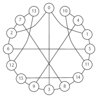
(a) ring layout

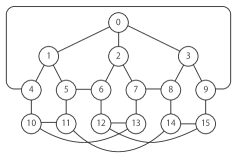
(b) pentagon (5-node cycle) layout

Figure 1: The best known graph with order $n=16$ and degree $d=4$

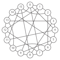
(a) ring layout

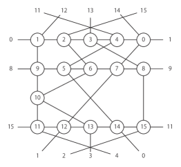
(b) pentagon (5-node cycle) layout

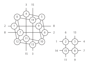
(c) square (4-node cycle) layout

Figure 2: The best known graph with order $n=10$ and degree $d=3$

III Heuristic Algorithm

III-A Policy and Outline of Heuristic Algorithm

Based on the observation of small order graphs described in Sec. II, we determine the outline of our heuristic algorithm as following two steps. 1) If target diameter is $k$, we connect small order graphs such that their diameter is $k-1$. For example, if the target diameter $k=3$ and order $n=10000$, the $1000$ Petersen graphs (Fig. 3, diameter $k=2$) are connected. 2) We try to increase the number of $(2k-1)$-node cycles, when edges are added. For graphs of $k=3$, we try to increase the number of pentagons (5-node cycles).

Outline of our heuristic algorithm is shown in Algorithm 1. In the remaining of the paper, we discuss only $k=3$ graphs. Our algorithm generates a graph which diameter is almost 3, for given order and degree.

Algorithm 1 Outline of graph generation algorithm

1:procedure GraphGenerater(order $n$, degree $d$)

2:     Create a base graph $G_{0}$, such that order of $G_{0}$ is $n$

3:     Create a graph $G$, by greedily adding edges one by one to $G_{0}$

4:     Return the graph $G$

5:end procedure

III-B Create a Base Graph $G_{0}$

A base graph $G_{0}=(V,E_{0})$ has $n$ nodes, i.e. $|V|=n$. The graph $G_{0}$ is a connected graph, but its degree is five. Most nodes have five edges. Other nodes, i.e., some border and anomalous nodes have four edges.

Graph $G_{0}$ contains multiple Petersen graphs. The Petersen graph $G_{P}$, which is shown in Fig. 3, is one of well-known Moore graphs [3], and has ten nodes and degree $d=3$. The diameter of Petersen graph is two. When the nodes are numbered in Fig. 3, fifteen edges of the Petersen graph are described as follows, for $i\in\{0,1,2,3,4\}$ and $j\in\{5,6,7,8,9\}$.

$$(i,i+1{\rm\;mod\;}5)$$

$$(i,(2i{\rm\;mod\;}5)+5)$$

$$(j,(j+1{\rm\;mod\;}5)+5)$$

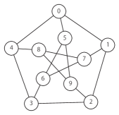
Figure 3: The Petersen graph $(n=10,d=3)$

If a given order $n$ is multiple of ten, we generate $(n/10)$ Petersen graphs, $G_{Pk}\;(k=1,2,3,\ldots,n/10)$. Adjacent Petersen graphs, $G_{Pk}$ and $G_{P(k+1)}$, are connected as shown in Fig. 4 by Connect procedure in Algorithm 2. Fig. 4 shows only edges crossing two Petersen graphs. In the case of $n=10000$, we generate 1000 Petersen graphs, and $k$-th graph are connected with $(k-1)$-th and $(k+1)$-th graph for $1<k<1000$.

Algorithm 2 Create a base graph $G_{0}$

1:procedure CreateBaseGraph($n$)

2:     for each $k\in\{1,\ldots,(n/10)\}$ do

3:         Create $k$-th petersen graphs

4:     end for

5:     for each $k\in\{1,\ldots,(n/10)-1\}$ do

6:         Connect$(k)$

7:     end for

8:end procedure

9:procedure Connect($k$)

10:     Connect $k$-th and $(k+1)$-th Petersen graphs as shown in Fig. 4

11:end procedure

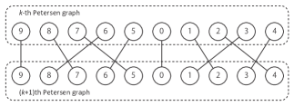
Figure 4: Connecting two adjacent Petersen graphs

When there is a remainder $r>0$ divided by ten, i.e., $n=10\cdot\lfloor n/10\rfloor+r$, we replace $r$ Petersen graphs with $r$ 11-node graphs. The 11-node graph is the subgraph of Fig. 2. We heuristically select eleven nodes, $5,6,7,\ldots,15$ from the graph of Fig. 2. When we connect a 11-node graph with adjacent Petersen graphs, we ignore node 10 and other ten nodes are connected similar to Fig. 4. The eleven nodes graph is shown in Fig. 5, nodes are renumbered, except for node 10. Nodes $5,6,7,8,9,11,12,13,14,15$ in Fig. 2 are renumbered to $2,3,4,0,1,6,7,8,9,5$ in Fig. 5, respectively.

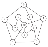
Figure 5: The 11-node graph $(n=11,d=4)$ for base graphs

The base graph $G_{0}$ is generated by CreateBaseGraph procedure in Algorithm 2. The base graph $G_{0}$ has $n$ nodes. Each node of $G_{0}$ has five edges, except for nodes in the first and the last Petersen graphs and node 10 of 11-node graphs. These exceptional nodes have just four edges.

III-C Greedily Add Edges One by One to $G_{0}$

In this step, we greedily add edges one by one to the base graph $G_{0}$. Our policies to add edges are the followings.

1. Increase the number of pentagons in the graph, to create a graph such that its diameter becomes three and its ASPL is close to two.

2. Add an edge, which has the smallest degree node on one side.

3. No track back, i.e., never remove edges from the graph.

Under the policy 1), our heuristic searches two nodes such that distance of them is four, and adds an edge between these two nodes. By adding the edge, the number of pentagons is increased. Even if the small-degree graph of $n=16$ and $d=4$ in Fig. 2, there are many pentagons those include a particular edge. For example, an edge 1-2 is contained in eight pentagons; 1-2-3-4-0, 1-2-6-7-0, 1-2-15-14-0, 1-2-3-8-9, 1-2-3-13-12, 1-2-6-5-9, 1-2-6-7-12, and 1-2-6-10-9.

The policy 2) is employed to uniformly increase the degree of nodes and save computation time. Our heuristic maintains the nodes that have the smallest degree, and selects a node from them as one side of a new edge. A node of the other side is selected based on the policy 1). Although we can select the new edge from all possible pair of nodes, to save computation time, our heuristic limits search space by fixing one side of new edge.

The policy 3) also saves computation time. As another reason, we do not find any effective evaluation function to track back.

Here, we explain this step in Algorithm 3. In each loop iteration of lines 3 to 17, two nodes $i$ and $j$ are selected and add an edge $i$-$j$ to the graph. Node $i$ is chosen from the nodes of the smallest degree in $G$ at line 4, based on policy 2). $d(i,j)$ denotes the distance between two nodes $i$ and $j$. In the loop of lines 6 to 14, candidates of node $j$ are evaluated, based on policy 1). After evaluation, node $j$ that satisfies two following conditions (1) and (2) is selected in line 15, and an edges $i$-$j$ is added to graph $G$ in the next line. $J^{\prime}$ is the subset of $J$ such that each node in $J^{\prime}$ satisfies condition (1). We have no particular tie-breaking rule.

$$p_{1}(j) = \min_{j^{\prime}\in J}p_{1}(j^{\prime})$$ (1)

$$p_{2}(j) = \max_{j^{\prime}\in J^{\prime}}p_{2}(j^{\prime})$$ (2)

The CountPaths function is used for the evaluation of $j\in J$. CountPaths$(i,j)$ roughly counts the number of paths between two nodes $i$ and $j$, those distance are three. $D_{m}(i)$ is the set of nodes distant $m$ from node $i$, i.e., for every node $k\in D_{m}(i)$, $k$ satisfies $d(i,k)=m$. For example, every node $k\in D_{1}(i)\cap D_{2}(j)$ satisfy $d(i,k)=1$ and $d(k,j)=2$. $p$ in line 21 is close to the twice of the number of 4-node paths.

Algorithm 3 Greedily add edges, one by one to $G_{0}$

1:procedure AddEdges($n,d,G_{0}$)

2:     $G\leftarrow G_{0}$

3:     while edge can be added do

4:          Select a node $i$ from the smallest degree nodes

5:         Compute node set $J$ such that $d(i,j)>2$

6:         for each node $j\in J$ do

7:              $p_{1}(j)=\mbox{\sc CountPaths}(i,j)$

8:              $p_{2}(j)=0$

9:              for each $k\in j$’s neighbors do

10:                  if $\mbox{\sc CountPaths}(i,k)>p_{2}(j)$ then

11:                       $p_{2}(j)=\mbox{\sc CountPaths}(i,k)$

12:                  end if

13:              end for

14:         end for

15:         Select $j\in J$ that satisfies conditions (1) and (2)

16:         Add an edge $i$-$j$ to graph $G$

17:     end while

18:     If degree of several nodes are less than $d$, add several edges between them

19:end procedure

20:function CountPaths($i,j$)

21:     $p=|D_{1}(i)\cap D_{2}(j)|+|D_{2}(i)\cap D_{1}(j)|$ $\triangleright$ Roughly count the number of paths with distance 3 between node $i$ and $j$, for graph $G$

22:end function

III-D Generated Graphs

Diameter $k$ and ASPL $l$ of generated graphs are shown in Table I. Fortunately, two graphs of $n=4096$ are the new records in the competition. The graph of $n=256$ has the same diameter, but longer ASPL than the best record $l=2.09262$ and two competitors’ records. For two graphs of $n=10000$, our first implementation is too slow and can not finish before the deadline of the 2015 competition. After the competition, we reimplement the program and get the results as shown in Table I.

TABLE I: Graphs generated by the heuristic algorithm

order $n$	degree $d$	diameter $k$	ASPL $l$	note
256	16	3	2.12757	not submitted
4096	60	3	2.295275	*1
4096	64	3	2.242228	*1
10000	60	3	2.648980	*2
10000	64	3	2.611310	*3
*1: None submits smaller graph in the competition. *2: A smaller-ASPL graph is created after competition. The winner’s graph of the competition has $l=2.650157$. *3: The graph is created after competition. However, the winner’s graph of the competition ($l=2.609927$) has smaller ASPL than this.

IV A Technique of 2-Opt Local Search

IV-A Edge Importance Function

After a graph is created by heuristic algorithm described in Sec. III for a given order and degree, we start 2-opt local search. 2-opt is the basic and widely used local search heuristic [8]. It is used for traveling salesperson problem (TSP) and others.

In this section, we explain edge importance which is used to prioritize edge combinations for 2-opt local search. 2-opt algorithm slightly modifies a given graph recursively. The modification of 2-opt is swapping two edges. An example of swapping two edges $a$-$b$ and $c$-$d$ into $a$-$d$ and $b$-$c$ is shown in Fig. 6. Diameter and ASPL of pre-swap graph $G=(V,E)$ and post-swap graph $G^{\prime}=(V,E^{\prime})$ are compared with each other. If diameter and/or ASPL of $G^{\prime}$ is smaller than $G$, this swap is accepted.

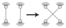
Figure 6: Swap two edges $a$-$b$ and $c$-$d$ into $a$-$d$ and $b$-$c$. (We assume degree $d=9$ and other nodes are not drawn. There is another swap into $a$-$c$ and $b$-$d$ for these edges)

2-opt local search is time-consuming task. There are many ways to reduce computation time. Even if we search a graph of order $n=256$ and degree $d=16$, there are 2048 edges in the graph. The number of edge pairs is about $2\times 10^{6}$. Generally, the number of edge pairs is about $\frac{nd}{2}\cdot\frac{(n-2)d}{2}\cdot\frac{1}{2}=O(n^{2}d^{2})$. For each swapped graph, we need to calculate diameter and ASPL. We adopt two techniques to save computation time. One is edge importance, and the other is fast ASPL calculation for 2-opt.

Our edge importance (or edge impact) is a value given to each edge of a graph. As an intuitive explanation, less important edges probably be removed from the graph with little increase of ASPL than other edges. Then, we give higher priority to less important edges, when we select an edge pair for swap.

The edge importance of an edge $e=j$-$k$ is defined by the following function.

$$f(e)=f(j\mbox{-}k)=\sum_{i\in V}f_{1}(i,j\mbox{-}k),$$

where $f_{1}(i,j\mbox{-}k)$ is the importance of edge $j$-$k$ for node $i$. The examples of $f_{1}(i,j\mbox{-}k)$ is shown in Fig. 7. We assume $f_{1}(i,j\mbox{-}k)=f_{1}(i,k\mbox{-}j)$ (symmetricity) and divide two cases of $f_{1}(i,j\mbox{-}k)$ as follows.

• If two nodes $j$ and $k$ have the same distance from $i$, i.e., $d(i,j)=d(i,k)$, then $f_{1}(i,j\mbox{-}k)=0$. (left of Fig. 7)

• If two nodes $j$ and $k$ have the different distance from $i$, i.e., $d(i,j)+1=d(i,k)$, then $0<f_{1}(i,j\mbox{-}k)\leq 1$. We define node set $J$, each of which has an edge to $k$ and its distance from $i$ is equal to $d(i,j)$.

  $$J=\{j^{\prime}|j^{\prime}\in V\mbox{ and }d(i,j^{\prime})=d(i,j)\mbox{ and }d(j^{\prime},k)=1\}$$

  Using $J$, $f_{1}(i,j\mbox{-}k)$ is defined as follows.

  $$f_{1}(i,j\mbox{-}k)=\frac{1}{|J|}$$

  The center of Fig. 7 shows a subcase of $|J|=2$, and the right of it shows the other subcase of $|J|=1$. Note that, this case includes the case of $i=j$. If $i=j$, then $|J|=1$ by the definition.

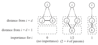
Figure 7: Edge importance of an edge $j$-$k$ for node $i$

IV-B Order of Edges Pairs for Local Search

Two lower-importance edges are the candidate of swapping for 2-opt local search. All edges are sorted by edge importance and denoted by $e_{0},e_{1},\ldots,e_{|E|-1}$. The edge $e_{0}$ has the smallest importance.

The 2-opt local search algorithm is shown in Algorithm 4 The loop of lines 5 to 11 is the main loop of local search. Line 6 is the important point using edge importance. We tries several orders to select a pair, which are described in the next paragraph. For pair $e_{i}(=a$-$b)$ and $e_{j}(=c$-$d)$ selected in line 6, there are two combinations of swapping, 1) $a$-$c$ and $b$-$d$ ($G^{\prime}$ of line 7) and 2) $a$-$d$ and $b$-$c$ ($G^{\prime\prime}$ of line 9) . Diameter and ASPL of both $G^{\prime}$ and $G^{\prime\prime}$ are calculated. The loop of lines 4 to 13 implies that edge importance is reused for swapped graphs. In our experience, after fifty swaps, ordering still valuable to find smaller ASPL graph.

Algorithm 4 2-opt local search

1:procedure Multiple2opt($G$)

2:     Calculate edge importance of all edges in $G$

3:     Sort edges by edge importance

4:     while timeout do

5:         repeat

6:              Select an edge pair $(e_{i},e_{j})$ in a particular order

7:              Generate swapped graph $G^{\prime}$

8:              Calculate diameter and ASPL of $G^{\prime}$

9:              Generate another swapped graph $G^{\prime\prime}$

10:              Calculate diameter and ASPL of $G^{\prime\prime}$

11:         until $G^{\prime}$ or $G^{\prime\prime}$ has smaller diameter or ASPL than $G$

12:         Copy $G^{\prime}$ or $G^{\prime\prime}$ to $G$

13:     end while

14:end procedure

We heuristically employ two searching orders of line 6 in Algorithm 4. Both orders satisfy $(e_{i},e_{j})<(e_{i},e_{k})<(e_{j},e_{k})$ for $i<j<k$. We think the order of the smallest first is better than it of triangle, empirically.

• the smallest first: $(e_{i},e_{l})<(e_{j},e_{k})$ for $i<j<k<l$.

  $(e_{0},e_{1}),(e_{0},e_{1}),(e_{0},e_{2}),\ldots,(e_{0},e_{|E|-1}),$
  $(e_{1},e_{2}),(e_{1},e_{3}),(e_{1},e_{4}),\ldots,(e_{1},e_{|E|-1}),$
  $(e_{2},e_{3}),(e_{2},e_{4}),(e_{2},e_{5}),\ldots,(e_{2},e_{|E|-1}),$
  $\ldots,$
  $(e_{i},e_{i+1}),(e_{i},e_{i+2}),(e_{i},e_{i+3}),\ldots,(e_{i},e_{|E|-1}),$
  $\ldots$

• triangle: $(e_{i},e_{l})>(e_{j},e_{k})$ for $i<j<k<l$.

  $(e_{0},e_{1}),$
  $(e_{0},e_{2}),(e_{1},e_{2}),$
  $(e_{0},e_{3}),(e_{1},e_{3}),(e_{2},e_{3}),$
  $\ldots,$
  $(e_{0},e_{i}),(e_{1},e_{i}),(e_{2},e_{i}),\ldots,(e_{i-1},e_{i}),$
  $\ldots$

Since ASPL calculation is time-consuming task, we additionally design ASPL recalculation method for 2-opt local search. The method stores the distance matrix of graph $G$ and update the matrix for swapped graph $G^{\prime}$. We can elimiate re-calculation of the distance between nodes which the swap does not affect.

IV-C Graph Instances

We run local search program during the competition and after competition. We show the smallest graph that we found in Table II. These graphs probably are the best-known graphs for these four combinations of order and degree. For graphs of order $n=4096$ and $n=10000$, Algorithm 4 is directly applied.

TABLE II: Graphs by local searching after 2015 competition

order $n$	degree $d$	diameter $k$	ASPL $l$	$l$ of Table I
256	16	3	2.09069	2.12757
4096	60	3	2.295216	2.295275
4096	64	3	2.242170	2.242228
10000	60	3	2.648977	2.648980
Note: all graphs may be the best-known graphs. The winner’s graph of the competition has larger ASPL than these.

For the graph of order $n=256$ and degree $d=16$, our graphs fall into local optimal many times. To find graphs of smaller ASPL, we accept worse post-graph $G^{\prime}$ than pre-swap graph $G$ in 2-opt local search. Fig. 8 shows the search history of the last 1000 graphs before reaching the best-known graph of $l=2.09069$. Many branches from each graph is omitted. In this figure, we show ASPL of each graph and order of edges that we swapped. The order of swapped edges is distributed from 0 to 620, i.e., swapped edges are two of $e_{0},e_{1},e_{2},\ldots,e_{620}$ in each graph. To reach the best-known graph, we need to run local search at least in the range of edge pair $(e_{i},e_{j})$ for $0\leq i\leq 153$ and $1\leq j\leq 620)$. This range contains only 4 % of all edge pairs. So, the edge importance seems to be valuable function to prioritize edges for swapping. We briefly explain the distribution of order of swapped edges. Since two edges are selected for each swap in Fig. 8, the total number of selected edges are 2000 for 1000 swaps. The half of these edges have the order smaller than 8. The order smaller than 108 contains 90% of these edges.

(a) first half (ASPL: $2.09163<l<2.09277$)

(b) last half (ASPL: $2.09068<l<2.09186$)

Figure 8: Local search history of 1000 graphs of order $n=256$ and degree $d=16$

V Conclusion

In this paper, we explained the heuristic algorithm that creates a graph which has small average shortest path length (ASPL) for diameter 3 graphs. The algorithm intends to increase the number of pentagons (5-node cycles). Through the observation of small order graphs which has diameter 3, we focused on the number of pentagons. The heuristic algorithm can create two best-known graphs at the graph golf 2015 competition, and a best-known graph after the competition. These three graphs have order $n=4096$ and degree $d=60$, $n=4096$ and $d=64$, and $n=10000$ and $d=60$.

We also explained the technique of 2-opt local search to reduce ASPL of a graph. The technique is based on the evaluation function called edge importance (or edge impact). Edges which have smaller importance compared to other edges are the good candidates for swap of 2-opt. We applied this technique to the graph of $n=256$ and $d=16$, and find a best-known graph after competition.

As future work, we will try to find more elegant heuristic to create a small ASPL graph, for not only diameter 3 graphs but also larger diameter graphs. Data structures for fast ASPL computation also should be explored.

References

- [1] P. Erdös, S. Fajtlowicz, and A.J. Hoffman, “Maximum Degree in Graphs of Diameter 2,” Networks, vol. 10, pp. 87–90, John Wiley & Sons, 1980.
- [2] E. Loz and J. Širáň, “New Record Graphs in the Degree-Diameter Problem,” Australasian Journal of Combinatorics, vol. 41, pp. 63–80, 2008.
- [3] M. Miller and J. Širáň, “Moore Graphs and Beyond: A Survey of the Degree/Diameter Problem,” Electronic Journal of Combinatorics, vol. 20, no. 2, #DS14v2, 92 pages, 2013.
- [4] G. Exoo and R. Jajcay, “Dynamic Cage Survey,” Electronic Journal of Combinatorics, #DS16, 55 pages, 2013.
- [5] M. Koibuchi, I. Fujiwara, S. Fujita, K. Nakano, T. Uno, T. Inoue, and K. Kawarabayashi, “Graph Golf: THe Order/degree Problem Competition,” http://research.nii.ac.jp/graphgolf/
- [6] M. Besta and T. Hoefler, “Slim Fly: A Cost Effective Low-Diameter Network Topology,” Proc. of International Conference on High Performance Computing, Networking, Storage and Analysis (SC ’14), pp. 348–359, Nov. 2014.
- [7] H. Matsutani, M. Koibuchi, I. Fujiwara, T. Kagami, Y. Take, T. Kuroda, P. Bogdan, R. Marculescu, and H. Amano, “Low-Latency Wireless 3D NoCs via Randomized Shortcut Chips,” Proc. of the conference on Design, Automation & Test (DATE ’14), Mar. 2014.
- [8] M. Englert, H. Röglin, and B. Vöcking, “Worst Case and Probabilistic Analysis of the 2-Opt Algorithm for the TSP,” Proc. of 18th annual ACM-SIAM symposium on Discrete algorithms (SODA ’07), pp. 1295–1304, Jan. 2007.