A local order metric for condensed phase environments

Abstract

We introduce a local order metric (LOM) that measures the degree of order in the neighborhood of an atomic or molecular site in a condensed medium. The LOM maximizes the overlap between the spatial distribution of sites belonging to that neighborhood and the corresponding distribution in a suitable reference system. The LOM takes a value tending to zero for completely disordered environments and tending to one for environments that match perfectly the reference. The site averaged LOM and its standard deviation define two scalar order parameters, $S$ and $\delta S$, that characterize with excellent resolution crystals, liquids, and amorphous materials. We show with molecular dynamics simulations that $S$, $\delta S$ and the LOM provide very insightful information in the study of structural transformations, such as those occurring when ice spontaneously nucleates from supercooled water or when a supercooled water sample becomes amorphous upon progressive cooling.

I Introduction

There is great interest in understanding the atomic scale transformations in processes like crystallization, melting, amorphisation and crystal phase transitions. These processes occur via concerted motions of the atoms, which are accessible, in principle, from molecular dynamics simulations but are often difficult to visualize in view of their complexity. To gain physical insight in these situations, it is common practice to map the many-body transformations onto some space of reduced dimensionality by means of functions of the atomic coordinates called order parameters (OPs), which measure the degree of order in a material.

Widely used OPs are the bond order parameters $Q_{l}$ steinhardt_bond-orientational_1983 that measure the global orientational order of a multiatomic system from the sample average of the spherical harmonics associated to the bond directions $\hat{\bf{r}}$ between neighboring atomic sites, typically the nearest neighbors. The average spherical harmonics $\bar{Y}_{lm}\equiv\left<Y_{lm}\left(\hat{\bf{r}}\right)\right>$ depend on the choice of the reference frame but the bond order parameters $Q_{l}\equiv\left[\frac{4\pi}{2l+1}\sum_{m=-l}^{l}\left|\bar{Y}_{lm}\right|^{2}\right]^{1/2}$ are rotationally invariant and encode an intrinsic property of the medium. The non-zero integer $l$ specifies the angular resolution of the bond order parameter, with $l=6$ being a standard choice. The $Q_{l}$’s take characteristic non zero values for crystalline structures and distinguish unambiguously crystals from liquids and glasses. In fact the $Q_{l}$’s vanish in the thermodynamic limit for all liquids and glasses, i.e. systems that lack long-range order and are macroscopically isotropic. Liquids and glasses, however, can differ among themselves in the short- and/or intermediate-range order. Some substances, like e.g. water, exhibit polyamorphism, which means that they can exist in different amorphous forms depending on the preparation protocol. In these cases we would need either a measure of the local order or a measure of the global order that could recognize different liquids and glasses. A good measure of the local order is also crucial to analyze heterogeneous systems, such as e.g. when different phases coexist in a nucleation process. Specializing the definition of the bond order parameters $Q_{l}$ to the local environment of a site $j$ is straightforward: it simply involves restricting the calculation of the average spherical harmonics to the environment of $j$, obtaining in this way local bond order parameters called $q_{l}(j)$ tenWolde_numerical_1995 . However, the $q_{l}(j)$’s are not as useful as their global counterparts, the $Q_{l}$’s, because they have limited resolution and liquid environments often possess a high degree of local order that make them rather similar to disordered crystalline environments mickel_shortcomings_2013 . Several approaches have been devised to improve the resolution of the measures of the local order tenWolde_numerical_1995 ; tenWolde_numerical_1996 ; tenWolde_homogeneous_1999 ; lechner_accurate_2008 ; ghiringhelli_state_2008 ; li_homogeneous_2011 ; kesserling_finite_2013 . For example, it has been suggested using combinations of two or more local OPs lechner_accurate_2008 ; volkov_molecular_2002 ; moroni_interplay_2005 ; desgranges_crystallization_2008 ; li_homogeneous_2011 ; russo_new_2014 ; sanz_homogeneous_2013 , but these approaches may still have difficulties in distinguishing crystalline polymorphs such as e.g. cubic (I$c$) and hexagonal (I$h$) ices. In these situations additional analyses may be needed or one may resort to especially tailored OPs steinhardt_icosahedral_1981 . Examples of the latter in the context of tetrahedral network forming systems are the local structure index (LSI) shiratani_growth_1996 ; shiratani_molecular_1998 , the tetrahedral order parameter $q_{th}$ uttomark_kineticks_1993 ; chau_a_new_1998 ; errington_relationship_2001 , and the interstitial site population russo_understanding_2013 .

Recently, an alternative approach to measure the local order in materials has been discussed in the literature, inspired by computer science algorithms known as $"$shape matching$"$ keys_characterizing_2011 . In these schemes the similarity between an environment and a reference is gauged by a similarity kernel, or similarity matrix iacovella_icosahedral_2007 ; keys_complex_2011 , which is often represented in terms of spherical harmonic expansions that measure angular correlations, in a way independent of the reference frame. General theories of the similarity kernel in the context of structure classification in materials science have been presented in Refs keys_complex_2011 ; bartok_representing_2013 . Approaches based on similarity kernels have been applied successfully to a number of problems, including studies of the icosahedral order in polymer-tethered nanospheres iacovella_icosahedral_2007 , studies of the morphology of nanoparticles keys_complex_2011 , models of self-assembly keys_characterizing_2011 , studies of quasi-crystalline and crystalline phases of densely packed tetrahedra haji-akbari_disordered_2009 , and the prediction of the atomization energies of small organic molecules de_comparing_2016 ; bartok_representing_2013 .

The approach that we introduce here belongs to this general class of methods and is based on a similarity kernel of the Gaussian type bartok_representing_2013 to measure the overlap between a local structure and an ideal reference. In our scheme, the similarity kernel is not represented in terms of basis functions like the spherical harmonics, but is globally maximized by rotating the local reference after finding an optimal correspondence between the site indices of the environment and those of the reference. Specifically, we consider the configurations, i.e. the site coordinates, of a system of $N$ identical atoms. The $M$ neighbors of each site define a set of local patterns. The $M$ corresponding sites of an ideal crystal lattice constitute the local reference. Typically, we take $M$ equal to the number of the first and/or the second neighbors at each site. Each pattern defines not only a set of directions, but also a set of inter-site distances. Under equilibrium conditions the average nearest neighbor distance takes the same value, $d$, throughout the sample and we set the nearest neighbor distance in the reference equal to $d$. The maximal overlap of pattern and reference at each site $j$ constitutes our local order metric (LOM) $S(j)$.
Since the overlap is maximized with respect to both rotations of the reference and permutations of the site indices, the LOM is an intrinsic property of each local environment and is independent of the reference frame. The LOM approaches its minimum value of zero for completely disordered environments and approaches its maximum value of one for environments that match perfectly the reference. The LOM is an accurate measure of the local order at each site. It allows us to grade the local environments on a scale of ascending order defined by the maximal overlap of each environment with the reference. In terms of the LOM we define two novel global OPs: the average score $S$, i.e. the site averaged LOM, and its standard deviation $\delta S$. $S$ and $\delta S$ are scalar OPs that characterize ordered and disordered phases with excellent resolving power.

In the following, we give a quantitative definition of the LOM and report an algorithm for calculating it. We demonstrate that this algorithm maximizes the overlap between pattern and reference in a number of important test cases. Then, we illustrate how $S$ and $\delta S$ can be used to characterize solid and liquid phases of prototypical two- and three-dimensional Yukawa systems, and of three-dimensional Lennard-Jones systems. Next, we consider some more complex applications. In one of them we monitor the structural fluctuations of supercooled water at different thermodynamic conditions within the ST2 model for the intermolecular interactions stillinger_improved_1974 . In another we report a molecular dynamics study of the spontaneous crystallization of supercooled water adopting the mW model potential for the intermolecular interactions molinero_water_2008 , showing that the LOM and the two global OPs $S$ and $\delta S$ provide a more accurate description of the nucleation process than standard OPs. Finally, we report a molecular dynamics study of the glass transition in supercooled water within the TIP4P/2005 model for the intermolecular interactions abascal_general_2005 . This study shows that the new OPs can detect the environmental signatures of the freezing of the translational and of the rotational motions of the molecules.

The paper is organized as follows. In section II we present the method. Section III reports application to solid-liquid phase transition. In Section IV we apply the method to characterize the local order in water phases. Crystallization and amorphisation of supercooled water are discussed in Section V. Our conclusions and final remarks are presented in Section VI.

II Method

The local environment of an atomic site $j$ in a snapshot of a molecular dynamics or Monte Carlo simulation defines a local pattern formed by $M$ neighboring sites. Typically these include the first and/or the second neighbors of the site $j$. There are $N$ local patterns, one for each atomic site $j$ in the system. Indicating by $\mathbf{P}_{i}^{j}(i=1,M)$ the position vectors in the laboratory frame of the M neighbors of site $j$, their centroid is given by $\mathbf{P}_{c}^{j}\equiv\frac{1}{M}\sum_{i=1}^{M}\mathbf{P}_{i}^{j}$. In the following we refer the positions of the sites of the pattern to their centroid, i.e. $\mathbf{P}_{i}^{j}-\mathbf{P}_{c}^{j}\rightarrow\mathbf{P}_{i}^{j}$. The local reference is the set of the same $M$ neighboring sites in an ideal lattice of choice, the spatial scale of which is fixed by setting its nearest neighbor distance equal to $d$, the average equilibrium value in the system of interest. For each atomic site $j$ the centroid of the reference is set to coincide with the centroid of the pattern, but otherwise the reference’s orientation is arbitrary. Thus the positions vectors of the reference sites in the $j$ neighborhood relative to their centroid in the laboratory frame are given by $\mathbf{A}^{j}\mathbf{R}_{i}^{j}$ where $\mathbf{A}^{j}$ is an arbitrary rotation matrix about the centroid. The rotation matrix can be conveniently expressed in terms of three Euler angles $\theta,\phi$ and $\psi$ belonging to the domain $\Omega\equiv\left(0\leq\theta<\pi,0\leq\phi<2\pi,0\leq\psi<2\pi\right)$. The sites of the pattern and of the reference are labeled by the indices $i$ of the position vectors. While the indices of the reference sites are fixed, any permutation of the indices of the pattern sites is allowed. We denote by $i_{\mathcal{P}}$ the permuted indices of the pattern sites corresponding to the permutation $\mathcal{P}$ (if $\mathcal{P}$ is the identical permutation the pattern indices coincide with those of the reference). For a given orientation of the reference and a given permutation of the pattern indices we define the overlap $\mathcal{O}(j)$ between pattern and reference in the $j$ neighborhood by:

$$\mathcal{O}(j)\left[\theta,\phi,\psi;\mathcal{P}\right]=\prod_{i=1}^{M}\exp\left(-\frac{\left|\mathbf{P}_{i_{\mathcal{P}}}-\mathbf{A}^{j}\mathbf{R}_{i}^{j}\right|^{2}}{2\sigma^{2}M}\right)$$ (1)

Here $\sigma$ is a parameter that controls the spread of the Gaussian functions. Intuitively, $\sigma$ should be of the order of, but smaller than, $d$ for the overlap function to be able of recognizing different environments. In our applications we adopted the choice $\sigma=d/4$ , as we found, in several test cases, that the results are essentially independent of $\sigma$ when this belongs to the interval $d/4\leq\sigma\leq d/2$ . The LOM $S(j)$ at site $j$ is the maximum of the overlap function $\mathcal{O}(j)$ with respect to the orientation of the reference and the permutation of the pattern indices, i.e.:

$$S(j)=\max_{\theta,\phi,\psi;\mathcal{P}}\mathcal{O}(j)\left[\theta,\phi,\psi;\mathcal{P}\right]$$ (2)

The LOM is an intrinsic property of the local environment at variance with the overlap function $\mathcal{O}(j)$ that depends on the orientation of the reference and on the ordering of the sites in the pattern. The LOM satisfies the inequalities $0\leq S(j)\leq 1$. The two limits correspond, respectively, to a completely disordered local pattern ($S(j)\rightarrow 0$) and to an ordered local pattern matching perfectly the reference ($S(j)\rightarrow 1$). The LOM grades each local environment on an increasing scale of local order from zero to one. As a consequence of the point symmetry of the reference the overlap function defined in Eq. 1 has multiple equivalent maxima. We present in Sect II.1 an effective optimization algorithm to compute $S(j)$. We define two global order parameters based on $S(j)$. One is the average score $S$ or site averaged LOM:

$$S=\frac{1}{N}\sum_{j=1}^{N}S(j)$$ (3)

The other is the standard deviation of the score that we indicate by $\delta S$ :

$$\delta S=\sqrt{\frac{1}{N}\sum_{j=1}^{N}\left(S(j)-S\right)^{2}}$$ (4)

In the following sections of the paper we show with numerical examples that the score $S$ has excellent resolution and is capable of characterizing with good accuracy the global order of both crystalline and liquid/amorphous samples. The standard deviation of the score, $\delta S$, provides useful complementary information and can enhance the sensitivity of the measure of the global order in the context of structural transformations.

II.1 Optimization algorithm

The overlap function $\mathcal{O}(j)$ defined in Eq. 1 has $L$ equivalent maxima. Here $L$ is the number of proper point symmetry operations of the reference. If a maximum corresponds to the permutation $\bar{\mathcal{P}}$ of the pattern indices and to the Euler angles $(\bar{\theta},\bar{\phi},\bar{\psi})$, all the other distinct but equivalent maxima can be obtained from the known maximum by rotating the reference from the direction $(\bar{\theta},\bar{\phi},\bar{\psi})$ with the $L-1$ point symmetry operations different from the identity, and by updating correspondingly the permutations of the pattern indices. To compute $S(j)$ (Eq. 2) it is sufficient to locate only one of these maxima. In view of the point symmetry of the reference, it would be sufficient for that to explore only a fraction $1/L$ of the Euler angle domain $\Omega$, which we may call $\Omega/L$ , the irreducible domain of the Euler angles. In the present implementation, however, we opted to explore the full $\Omega$ domain for reasons of simplicity. We also notice that $\mathcal{O}(j)$ in Eq. 1 decays rapidly to zero when the distance between any one of the pattern sites and the corresponding reference site is sufficiently larger than $\sigma$.

To identify a permutation for which $\mathcal{O}(j)$ is in the neighborood of a maximum we proceed as follows. First, we represent the domain $\Omega$ on a uniform grid with $K/2\times K\times K$ points. Here $K$ is an even integer equal to the number of intervals dividing the range of each Euler angle. The grid points $(k_{1},k_{2},k_{3})$ with $(k_{1}=0,K/2-1,k_{2}=0,K-1,k_{3}=0,K-1)$, define the set of Euler angles $(\theta=2k_{1}\pi/K,\phi=2k_{2}\pi/K,\psi=2k_{3}\pi/K)$, the corresponding rotation matrices $\mathbf{A}^{j}$ and the associated reference vectors $\mathbf{A}^{j}\mathbf{R}_{i}^{j}$ that we shall use in Eq. 1. Next, we select an initial grid point, such as e.g. $(k_{1}=k_{2}=k_{3}=0)$. For this grid point we select a permutation $\mathcal{P}$ with the following algorithm: 1. Pick one of the $M$ pattern sites at random with uniform probability: let it be site $i^{\prime}$. 2. Compute the square distances $\left|\mathbf{P}_{i^{\prime}}^{j}-\mathbf{A}^{j}\mathbf{R}_{i}^{j}\right|^{2}$ between the pattern site $i^{\prime}$ and all the $M$ reference sites. 3. Set $i^{\prime}$ equal to the index of the reference site with the smallest distance from $P_{i^{\prime}}^{j}$. 4. Pick at random with uniform probability one of the remaining $M-1$ pattern sites and compare it with the remaining $M-1$ reference sites. 5. Set the index of the chosen pattern site equal to that of the reference site with the smallest distance from it. 6. Pick at random one of the remaining $M-2$ sites and compare it with the remaining reference sites in order to set its index. 7. Proceed in the same way until all the indices have been set. Having selected a permutation $\mathcal{P}$ we compute $\mathcal{O}(j)$ with Eq. 1. Then we move to a neighboring point on the grid of the Euler angles, e.g. $(1,0,0)$, repeat the above procedure to select a permutation of the indices starting from the permutation selected at the previous step, and compute the corresponding $\mathcal{O}(j)$. We repeat this procedure by moving systematically on the grid of the Euler angles (e.g. sample $k_{1}$ first, followed by $k_{2}$, and then by $k_{3}$). The largest $\mathcal{O}(j)$ calculated in this way is guaranteed to be in the basin of attraction of one of the equivalent maxima of $\mathcal{O}(j)$ and the subsequent optimization can be done with respect to the Euler angles only, while keeping the permutation of the indices fixed. This angular optimization is a local optimization problem and can be performed effectively with gradient methods, such as steepest descent or conjugate gradients.

In all our applications we adopted the choice $K=18$, which we found to be sufficient for good convergence. To check that the algorithm leads correctly to the maximum of $\mathcal{O}(j)$ we made several tests. In some of them we considered a perfect crystalline environment (at zero temperature) and chose a reference based on the same crystalline structure. In this case $S(j)$ should take the value $S(j)=1$. We found that this was always the case when starting from random permutations of the pattern sites and random orientations of the reference. In other tests we considered disordered crystalline and liquid environments at different temperatures. In these cases the exact values of $S(j)$ are not known a priori. However, in all the cases we found that $S(j)$ converged always to the same value within the tolerance of the convergence criterion, independently of the initial random values chosen for the permutation of the pattern indices and for the orientation of the reference.

In Fig. 1 a two-dimensional crystal with Yukawa pair interactions is used to illustrate the method. The system has been equilibrated at finite temperature. As reference we choose the $6$ sites associated to the second shell of neighbors in the ideal triangular lattice. The $6$ sites are the vertices of a regular hexagon. The picture shows (a) a local environment, (b) the corresponding reference with shaded areas representing the regions in the neighborhood of the reference selected by $\sigma$, (c) the optimal overlap between pattern and reference for the local environment depicted in (a).

Figure 1: Schematic representation of our approach in an application to a 2D Yukawa crystal at $k_{B}T/V_{0}=0.001$. a): The red spheres indicate the second shell of neighbors of site $j$ (yellow sphere). b): The $6$ blue spheres are the vertices of the reference hexagon. The green shaded areas represent the Gaussian domains. c): Optimized overlay of reference and local patterns.

III Applications to simple systems

As a first application we use the new OPs to analyze simulations of simple condensed phase systems at varying temperature. Initially the temperature is low and the systems are in the solid state. When the temperature exceeds a certain threshold, the solid looses mechanical stability and the atomic dynamics becomes diffusive signaling a transition to the liquid state. We have considered, in particular, the following systems: a 2D system of identical particles with Yukawa pair interactions, a 3D system of identical particles with Yukawa pair interactions, and a 3D system of identical particles with Lennard-Jones pair interactions. In all cases we find that the new OPs signal the transition to the liquid state with sensitivity equivalent to that of popular OPs, like $Q_{6}$ and its two-dimensional specialization $\Psi_{6}$ chakrabarti_effect_1998 . However, once in the liquid state our OPs can still quantify the degree of order and are therefore superior to $Q_{6}$ and $\Psi_{6}$.

III.1 Yukawa system in 2D

Here we perform Brownian dynamics simulations of particles with repulsive pair interactions given by the Yukawa potential $V(r)=V_{0}\exp(-\kappa r)/\kappa r$, where $r$ denotes the inter-particle separation, and $\kappa$ is the inverse screening length. The strength of the interaction is set by the amplitude $V_{0}$. We consider a system of $9180$ particles in the $NVT$ ensemble with periodic boundary conditions. We start the simulations from a perfect triangular lattice. We analyse the degree of local order as a function of $k_{B}T/V_{0}$ at the fixed reduced screening length $\rho/\kappa^{2}=0.21$, where $\rho$ is the 2D number density. Without loss of generality we hereby use $V_{0}=1$. Pattern sites comprise the second shell of neighbors and are compared with the reference in Fig. 1 for a representative snapshot of the solid at $k_{B}T/V_{0}=0.001$.

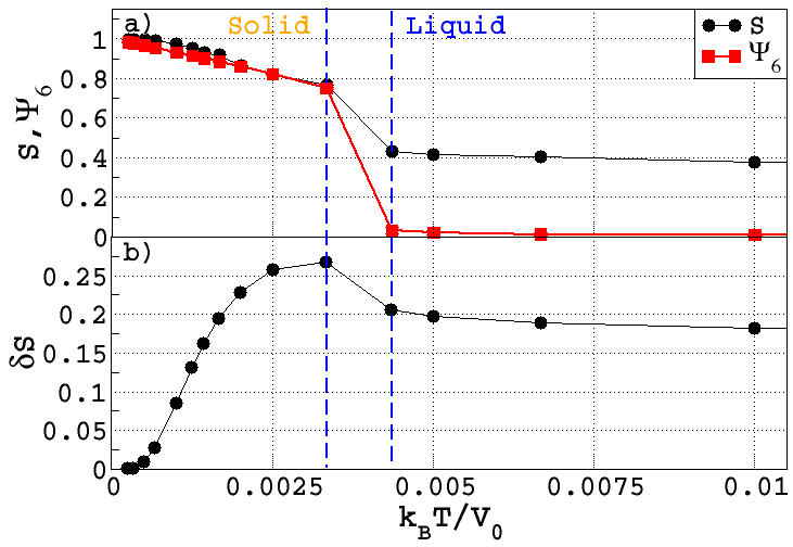
Figure 2: a): 2D Yukawa system. Profile of $S$ (black dots) and of $\Psi_{6}$ (red squares) as a function of $k_{B}T/V_{0}$. The blue dashed lines delimit the region of instability of the solid phase in the simulation. b): 2D Yukawa system. Profile of $\delta S$ as a function of $k_{B}T/V_{0}$.

Panel (a) of Fig. 2 compares the global OPs $S$ (black dots) and $\Psi_{6}$ (red squares). As expected, both $S$ and $\Psi_{6}$ for the perfect crystal take the value of $1$. As $T$ increases, both $S$ and $\Psi_{6}$ decrease. In correspondence with the blue dashed lines, signaling instability of the crystal, both OPs show a quick drop. In the liquid phase, $\Psi_{6}\simeq 0$, as expected, while $S$ keeps a finite value of $S\simeq 0.4$, which slightly decreases as the temperature is further increased. Therefore, both $S$ and $\Psi_{6}$ identify the phase transition, but only $S$ is able to quantify the degree of order remaining in the liquid phase.

The behavior of $\delta S$ in panel (b) gives further insight on the solid-liquid transition. $\delta S$ takes the maximum value in the crystal at the highest temperature and drops substantially in the liquid phase. This behaviour follows from the non linear nature of the LOM. The liquid phase has more strongly disordered local patterns with sites often belonging to the tails of the Gaussian domains in Eq. 1. Site fluctuations in the liquid weight less than fluctuations in the solid, where patterns sites are closer to the centers of the Gaussian domains.

We have observed the same behavior of $\delta S$ in all the solid-liquid transitions that we have investigated, namely $\delta S$ takes its maximum value in the hot crystal before the occurrence of the dynamical instability that signals melting. It is tempting to notice the similarity of this behavior with Lindemann’s melting criterion lindemann_calculation_1910 , according to which melting occurs when the average atomic displacement exceeds some fraction of the interatomic distance. In our approach the dynamic instability is associated to the largest fluctuation of $S$.

III.2 Yukawa and Lennard-Jones systems in 3D

In Fig. 3 we report $S$ and $Q_{6}$ as a function of the temperature for a 3D system of identical particles with Yukawa pair interactions (panels (a) and (b)) and for a 3D system of identical particles with Lennard-Jones pair interactions (panels (c) and (d)). At low temperature the Yukawa system is in the bcc crystalline phase whereas the Lennard-Jones system is in the fcc crystalline phase. In the Yukawa system we use the pairwise interactions introduced in Section III.1. We sample the $NVT$ ensemble with Brownian dynamics. The simulation cell contains $4394$ particles with periodic boundary conditions. The reference includes the first and the second shell of neighbors of a perfect bcc lattice for a total of $14$ sites. Panel (a) shows $S$ (black dots) and $Q_{6}$ (red squares) versus temperature. At very low temperatures, $S\simeq 1$ because reference and pattern overlap almost perfectly. Increasing the temperature, both OPs show a quick drop in correspondence with the phase transition with $Q_{6}\rightarrow 0$ as expected in the liquid phase, and $S$ taking a value $S\simeq 0.4$. Like in 2D, both order parameters are able to identify the phase transition, but $S$ provides quantitative information on the order present in the liquid, whereas $Q_{6}$ takes zero value in all liquids in the thermodynamic limit. It is worth recalling that local OPs, such as the $q_{l}(j)$, have difficulties in identifying the bcc symmetry of hot crystals before melting da-qi_structure_2005 . Our approach uses a non-linear LOM, which can unambiguously distinguish distorted local bcc structures from distorted local fcc or hcp structures. To illustrate this statement we report in the temperature range of crystalline stability in Fig. 3 (a) the profile of $S$ (green diamonds) obtained by using as reference the first shell of neighbors of the fcc lattice. We notice that $S$(bcc) and $S$(fcc) are well separated in the solid phase even at the highest temperatures. Panel (b) shows $\delta S$. As in 2D, $\delta S$ takes its maximum value in the solid phase before the onset of crystalline instability in the simulation.

In panels (c) and (d) we report the same data for a 3D system of identical particles interacting with the Lennard-Jones potential with parameters appropriate to Argon frenkel2001understanding . In this case we perform Monte Carlo simulations in the $NpT$ ensemble with a periodic box containing $1372$ particles. We choose as reference the anticuboctahedron, which has $12$ vertices, and corresponds to the first shell of neighbors in the ideal fcc lattice. The temperature variation of $S$ (black circles) and $Q_{6}$ (red squares) is shown in panel (c). At very low temperature, $S\simeq 1$ due to the nearly perfect overlap of patterns and reference. $S$ and $Q_{6}$ are able to distinguish the crystalline solid from the liquid, and show a substantial drop in correspondence with the dashed vertical blue lines. In the liquid, $Q_{6}\rightarrow 0$ as expected, while $S$ remains finite with a value close to $0.2$. Similarly, $\delta S$ in panel (d) takes its maximum value in the crystal at the highest temperature.

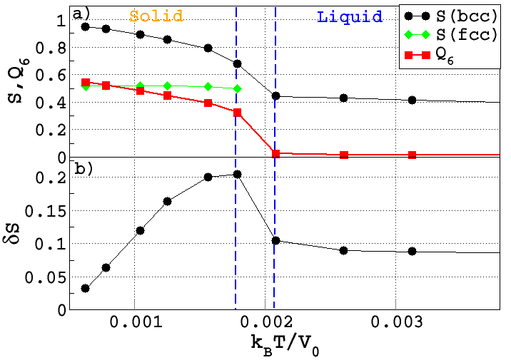
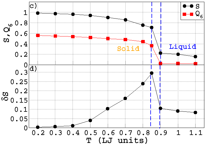
Figure 3: a): $S$ computed with ideal bcc crystal reference (black dots), $Q_{6}$ (red squares), and $S$ computed with fcc reference (green diamonds), as a function of $k_{B}T/V_{0}$ for a 3D Yukawa system. b): $\delta S$ corresponding to $S$ with bcc reference for the same Yukawa system. c): $S$ (black dots) and $Q_{6}$ (red squares) as a function of $T$ for a Lennard-Jones system. d): $\delta S$ for the same Lennard-Jones system. The vertical blue dashed lines delimit the regions of crystal instability in the simulations.

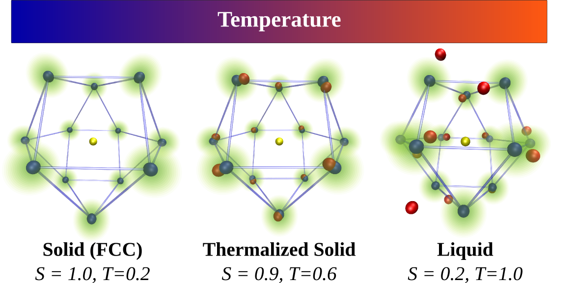
Figure 4: Local environments in solid and liquid Lennard-Jonesium at different temperatures. The notation is the same of Fig. 1. Neighboring reference sites have been connected by thin lines to emphasize the structure of the anticuboctahedron.

Representative local environments at different temperatures around a site indicated by a yellow sphere are shown in Fig. 4: the environment on the left corresponds to a cold crystal ($T=0.2$), the one in the middle to a hot crystal ($T=0.6$), and the one on the right to a liquid ($T=1.0$). One may notice the increasing deviation with temperature of the pattern sites (red spheres) relative to the reference sites (blue spheres). In the liquid state some of the pattern sites move in the tail region of the Gaussian domains, causing a drop in both $S$ and $\delta S$.

IV Local structures in water phases

Molecular systems like water exhibit a rich phase diagram, with two competitive crystalline phases, cubic (I$c$) and hexagonal (I$h$) ice, respectively, at low pressure. Moreover, metastable undercooled liquid water transforms continuously with pressure from a low-density form (LDL) to a high-density one (HDL) soper_structures_2000 . In the following we consider representative I$c$ and I$h$ solids, LDL and HDL liquids at different thermodynamic conditions.

Water molecules bind together by hydrogen bonds forming a tetrahedral network connecting neighboring molecules. To describe this network it is sufficient to consider the molecules as rigid units centered on the oxygens. The sites that define the local order are the oxygen sites and application of the formalism is straightforward. Water structures are dominated by tetrahedral hydrogen bonds and have similar short range order (SRO). The intermediate range order (IRO) is significantly more sensitive to structural changes than the SRO. We choose therefore references associated to the second shell of neighbors in crystalline ices. In particular, we adopt either the cuboctahedron $(C)$ or the anticuboctahedron $(\bar{C})$, both of which have $12$ vertices and correspond to the second shell of neighbors in cubic and hexagonal ices, respectively. In these simulations we used the ST2 force field stillinger_improved_1974 for water with periodic boundary conditions and adopted the Ewald technique (with metallic boundaries) to compute the electrostatic sums.

IV.1 Hexagonal and cubic ice

The simulation box for I$c$ ice is cubic and contains $512$ molecules, while that for I$h$ ice is orthorhombic and contains $768$ molecules. We thermally equilibrate both solids via classical MD simulations in the $NpT$ ensemble at $T=250$ K and $p=1$ bar. In panel (a) of Fig. 5 we report the distribution of $S$ with reference $\bar{C}$ indicated by $S_{\bar{C}}$ for cubic (black) and hexagonal (red) ices. In panel (b) of the same figure, we report the corresponding distributions of $S$ with reference $C$ indicated by $S_{C}$. It is clear from both panels that the distributions based on the two different references for the same crystal are well separated. Moreover, the distributions corresponding to the two different crystals are also well separated irrespective of the reference we use.

One notices in Fig. 5 that the distribution of the order parameter $S$ is broad when the reference is based on the same lattice of the pattern, i.e. $\bar{C}$ for I$h$ ice and $C$ for I$c$ ice. The distribution is instead rather sharp when the $\bar{C}$ reference is used to measure I$c$ patterns or when the $C$ reference is used to measure I$h$ patterns. This behavior is a consequence of the non-linearity of the LOM. When pattern and reference correspond to the same crystalline lattice the pattern sites are closer to the reference sites and small fluctuations in the pattern cause relatively large variations of the LOM. On the other hand, when pattern and reference do not correspond to the same crystalline lattice, pattern sites deviate more from the reference sites and small fluctuations in the pattern cause relatively small variations of the LOM.

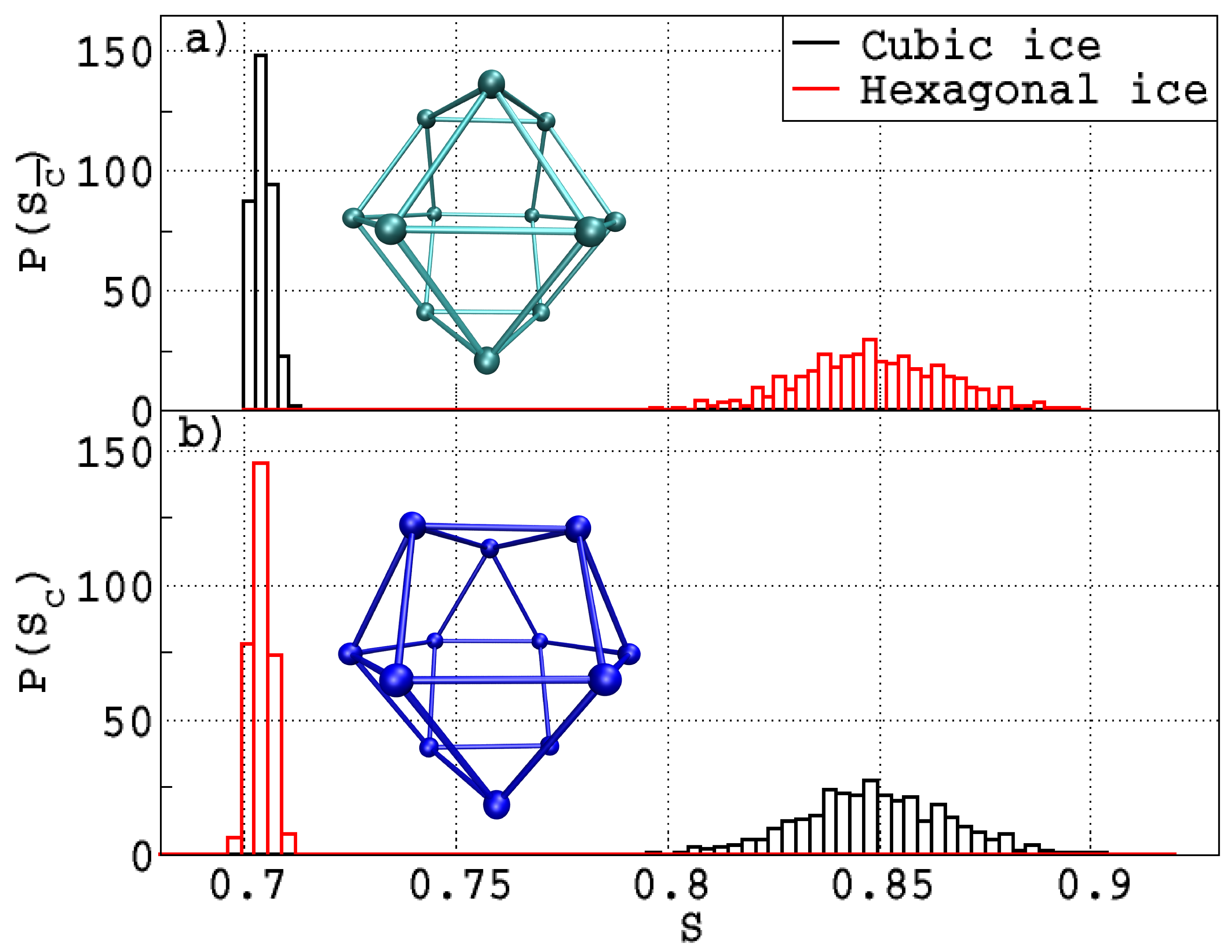
Figure 5: a): distribution of $S$ for I$c$ ice (black) and for I$h$ ice (red) with the $\bar{C}$ reference. b): distribution of $S$ for I$c$ ice (black) and for I$h$ ice (red) with the $C$ reference. The $\bar{C}$ and the $C$ references are depicted in the upper and in the lower panel, respectively. Spheres representing oxygen atoms are connected by sticks to emphasize the cuboctahedron (green) and the anticuboctahedron (blue).

IV.2 Low-density and high-density liquid water

We performed MD simulations for water in the $NpT$ ensemble at $T=240$ K and $p=1$ bar and $p=3$ kbar, respectively. The case $p=1$ bar is representative of a LDL liquid, while the case with $p=3$ kbar is representative of a HDL liquid. We use a cubic box containing $512$ molecules with periodic boundary conditions.

Resolving the local order in disordered structures, like HDL and LDL water, is difficult. Standard local OPs such as $q_{6}(j)$ fail in this respect and ad hoc OPs like the local structure index (LSI) have been devised for the task. The LSI is sensitive to the order in the region between the first two coordination shells of water. In this region the LSI detects the presence of interstitial molecules, whose population increases as the density or the pressure increases. While the LSI is an OP especially tailored for water, $S$ is non specific to water but has resolving power equivalent to that of the LSI in liquid water, as illustrated in Fig. 6. The two panels in this figure show the distribution of $S_{\bar{C}}$ (panel (a)) and of $S_{C}$ (panel (b) for HDL (black) and LDL (red). In both cases the distributions are well separated, similarly to the LSI distributions shown in the inset in panel (b). Independently of the adopted reference, $S$ has a higher value in LDL than in HDL, reflecting the higher degree of order in the former. By comparing the two panels in Fig. 6 we also see that both liquids have higher $\bar{C}-$ than $C-$character. Both LDL and HDL structures are well distinct from the crystalline reference and the corresponding broadening of the $S$ distributions is approximately the same in the two liquids.

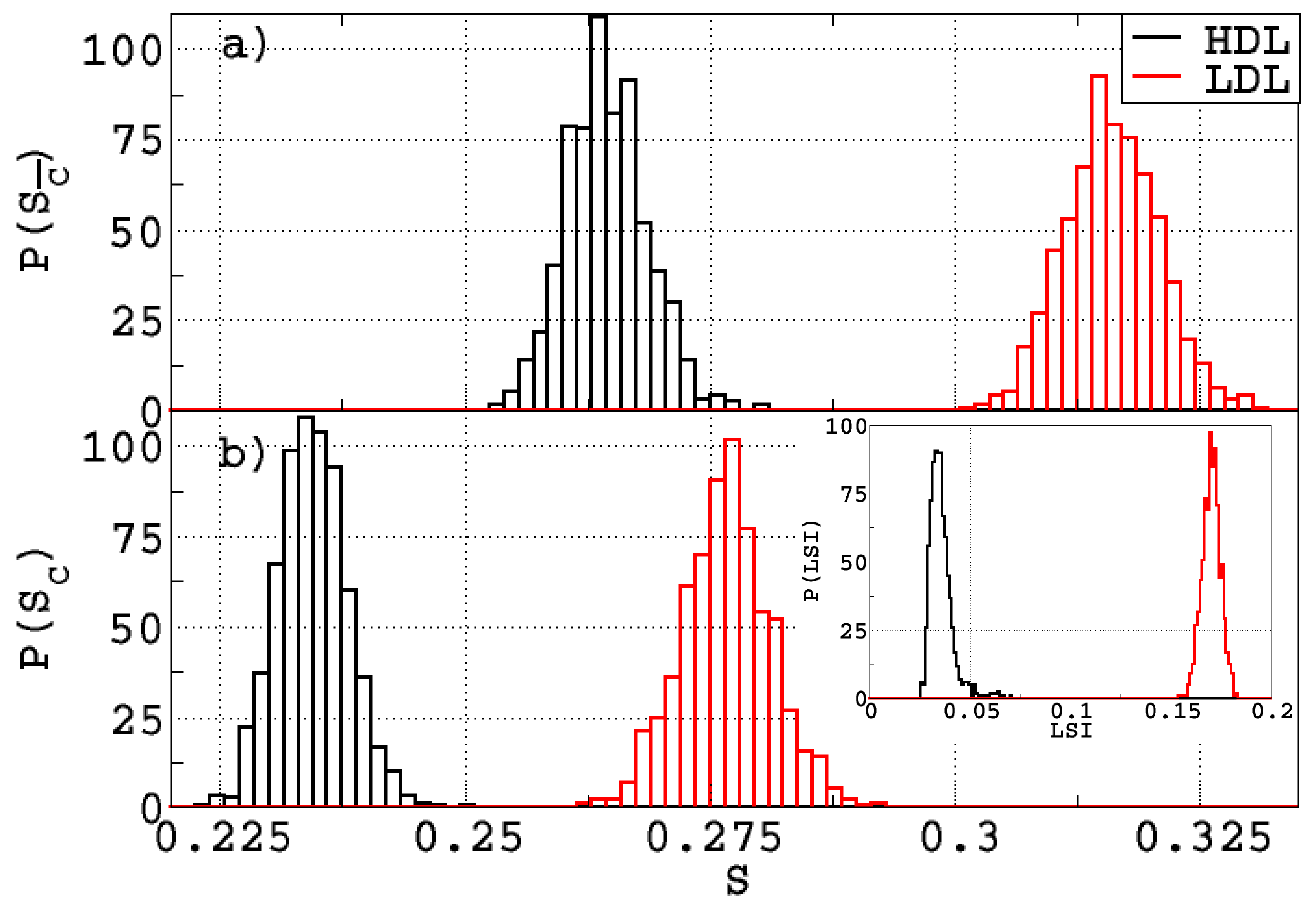
Figure 6: a): distribution of $S$ for HDL water (black) and for LDL water (red) with the $\bar{C}$ reference. b): distribution of $S$ for HDL water (black) and for LDL water (red) with the $C$ reference. The $\bar{C}$ and the $C$ references are depicted in Fig. 5. The inset shows the distribution of LSI for HDL water (black) and LDL water (red).

V Crystallization and amorphisation of supercooled water

To further illustrate the power of the LOM and of $S$ and $\delta S$ we consider the complex structural rearrangements occurring in supercooled water during crystallization or when a liquid sample amorphizes under rapid cooling.

To model crystallization, we consider rigid water molecules interacting with the mW potential molinero_water_2008 . The mW potential describes the tetrahedrality of the molecular arrangements, but does not have charges associated to it missing the donor/acceptor character of the hydrogen bonds. For that reason crystallization occurs much faster with mW than with more realistic potentials that describe more accurately the hydrogen bonds. At deeply supercooled conditions mW water crystallizes spontaneously on the time scale of our molecular dynamics simulations. In spite of the simplified intermolecular interactions in mW water, ice nucleation is a very complex process and access to good order parameters is essential to interpret the simulations.

To model amorphisation we adopt the more realistic TIP4P/2005 potential abascal_general_2005 for the intermolecular interactions. This potential applies to rigid molecules but takes into account the charges associated to the hydrogen bonds. This level of description is important to model the relaxation processes that occur in a liquid sample undergoing amorphisation. The processes that lead to the freezing of translational and rotational degrees of freedom in the glass transition are captured well by our OPs.

V.1 Crystallization of supercooled water

To study crystallization we performed classical MD simulations in the $NVT$ ensemble, using $1000$ molecules with interactions described by the mW potential molinero_water_2008 in a parallelepipedic box with side lengths ratios $L_{z}/L_{x}=4,L_{y}/L_{x}=1$, and periodic boundary conditions. We set the temperature to $T=190$ K and the volume of the box to a mass density of $\rho=0.98$g/cm³. At these thermodynamic conditions spontaneous crystal nucleation occurs rapidly in the mW fluid molinero_water_2008 . The evolution of the water sample starting from an equilibrated liquid is illustrated in Fig. 7,

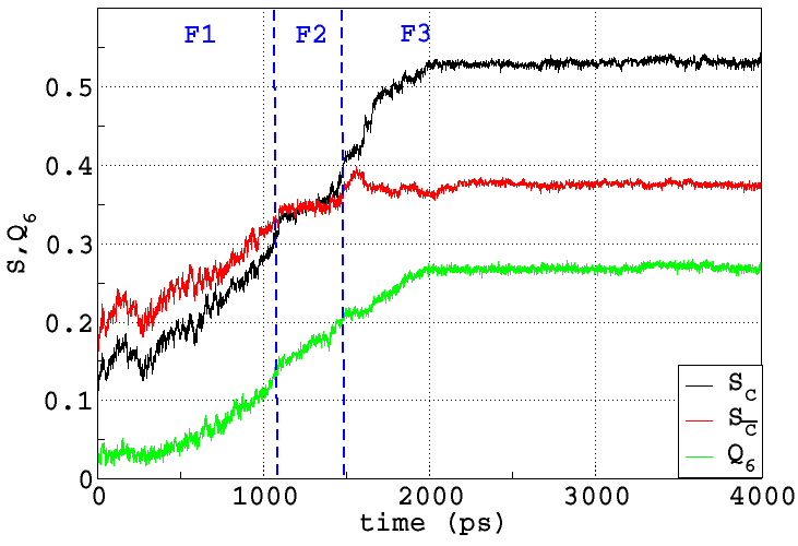
Figure 7: Comparison of $S_{C}$ (black), $S_{\bar{C}}$ (red), and $Q_{6}$ (green) as a function of time in the crystallization of $1000$ water molecule interacting via the mW potential. The blue vertical dashed lines indicate three time frames F1, F2, and F3, respectively.

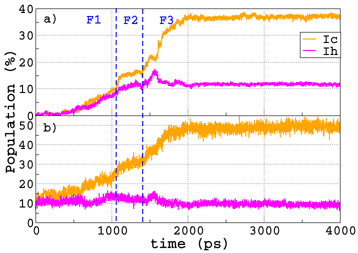
Figure 8: Time evolution during crystallization of mW water of the relative population of the sites with crystalline $I_{c}$ character (orange line) and of the sites with crystalline $I_{h}$ character, as determined from the LOM (a) and from $q_{6}/w_{4}$ (b). See text for a detailed explanation.

where we report the evolution with time of three OPs: $Q_{6}$ (green line), $S_{C}$ (black line) and $S_{\bar{C}}$ (red line), respectively. In this figure we recognize three time frames separated by the dashed vertical blue lines and indicated by F1, F2, and F3, respectively. In F1 the system is liquid but becomes increasingly structured as indicated by the growth of the three OPs. Microcystallites keep forming and disappearing. $S_{C}$ and $S_{\bar{C}}$ are more sensitive than $Q_{6}$ to the fluctuations of the local order, as indicated by the greater fluctuations of the black and red lines relative to the green line in F1. Interestingly, the liquid has stronger $\bar{C}-$ than $C-$character, in accord with Fig. 6. The relative weight of the $\bar{C}$- and $C$- characters reverses as crystallization proceeds. F2 marks the appearance of a stable crystallite that further grows in the initial stage of F3. This complex kinetics is not captured by $Q_{6}$ (green line) which shows only a continuous growth with time. Instead, both $S_{C}$ and $S_{\bar{C}}$ identify a plateau in F2, in correspondence with the formation of a stable crystallite.

The nucleating ice is a mixture of cubic and hexagonal ices, with a prevalence of the former, as indicated by the larger overall growth of $S_{C}$ in the simulation. Indeed, during the entire evolution shown in Fig. 7, $S_{C}$ varies more than $S_{\bar{C}}$. Due to $NVT$ sampling with periodic boundary conditions, liquid water is always present in the sample and does not disappear even when the nucleation process is completed in F3. The residual liquid water has more $\bar{C}-$ than $C$-character and, therefore, the $S_{C}$ and the $S_{\bar{C}}$ profiles should be considered merely as qualitative site-averaged contours.

More quantitative insight can be extracted from Fig. 8, where we report the time evolution of the fraction of cubic and hexagonal sites. This analysis is based on the LOM and is independent of the reference choice since distributions of the competing ice and liquid structures in Figs. 5 and  6 do not overlap. Thus, in the remaining part of this section and in Sect. VB as well, we use the $C$ reference and omit from $S$ the corresponding subscript. We introduce two cutoff values, $S_{1}=0.6$ and $S_{2}=0.75$, to distinguish the local environments. If at site $j$ the LOM satisfies $S^{j}<S_{1}$ the local environment is liquid-like, if $S_{1}<S^{j}<S_{2}$ the local environment is ice hexagonal-like, and if $S^{j}>S_{2}$ the local environment is ice cubic-like. Notice that the results do not depend on the actual values of the cutoffs $S_{1}$ and $S_{2}$ as long as they fall inside regions where the $S$ distribution has negligible weight. The time evolution of the fraction of sites with cubic and hexagonal character resulting from the LOM is reported in panel (a) of Fig. 8. In the F1 frame both cubic and hexagonal fractions grow with a slight dominance of the former. This growth is associated to crystallites that keep forming and disappearing. In correspondence with the first dashed vertical line the growth becomes faster for both environments, signaling the formation of a stable crystalline nucleus with mixed character, in which I$c$ and I$h$ sites are separated by a stacking fault. At this point hexagonal growth almost entirely stops while cubic ice continues to grow at a slower pace by incorporating nearby crystallites with the same character. The stable nucleus contains approximately $300$ out of $1000$ sites and takes the form of a large ice cluster embedded in a dominant liquid environment. Towards the end of the F2 frame, cubic ice growth accelerates and, in the early stage of the F3 frame, the size of the crystalline cluster rapidly reaches the size of the box. At this point no further growth is possible. In the early stage of F3 hexagonal growth is significantly less pronounced than cubic growth and is mainly associated to a visible hump shortly after the onset of F3. The hump is due to small clusters with hexagonal character that form on the surface of the large cubic crystallite, and then rapidly convert to cubic character. The nucleation ends with the formation of a large crystallite that spans the size of the box and includes $\sim 50\%$ percent of the available sites. Of the crystalline sites $\sim 80\%$ percent have cubic and $\sim 20\%$ percent hexagonal character. The quantitative details of the nucleation process depend on the MD trajectory. For instance the relative fraction of cubic and hexagonal sites changes from one trajectory to another. Qualitatively, however, the process is the same in all the 10 trajectories that we have generated. Our results are quantitatively very similar to a previous analysis in which cubic and hexagonal sites were identified in terms of eclipsed and staggered local configurations moore_freezing_2010 ; moore_is_2011 ; nguyen_identification_2015 . To further illustrate the superior resolving power of the LOM relative to common OPs we report in panel (b) of Fig. 8 an analysis of the same MD trajectory of panel (a) using a combination of the two orientational OPs $q_{6}(j)$ and $w_{4}(j)$ steinhardt_icosahedral_1981 . In this approach, $q_{6}(j)$ is extracted from the nearest neighbors of a site $j$ and serves to determine the liquid or the crystalline character of the site. If the site $j$ is crystalline one assigns to it cubic or hexagonal character depending on the value of $w_{4}(j)$, whose computation requires the first and second neighbors of the site $j$. There are important quantitative differences between panel (a) and panel (b) of Fig. 8. A major difference is already apparent in the time frame F1: in panel (b) a significant fraction of the sites that are considered liquid in panel (a) are classified as crystalline sites since the very beginning of the trajectory. This is due to the fact that liquid- and crystal-like configurations overlap in the $q_{6}$ distribution. Similarly, the relative fractions of cubic and hexagonal sites of panel (a) at the end of the trajectory is not reproduced well in panel (b), again because of the overlap of cubic and hexagonal configurations in the $w_{4}$ distribution.

V.2 Amorphisation of supercooled water

To study amorphisation, we have performed classical MD simulations for a system composed of $216$ molecules interacting via the TIP4P/2005 potential abascal_general_2005 in a cubic simulation box with periodic boundary conditions. Starting from an equilibrated liquid at $240$ K and $p=1$ bar, we performed isobaric cooling with a rate of $5$ K/ns to generate an amorphous ice structure. Given the adopted protocol this structure should have similarity to experimentally prepared low density amorphous (LDA) ice structures mayer_new_1985 . Our cooling rate is slightly higher then the one recently adopted in molecular dynamics simulations for the same water model wong_pressure_2015 . However, our goal is not to generate a high quality amorphous structure, but rather to test whether our approach can be used to study the glass transition in water.

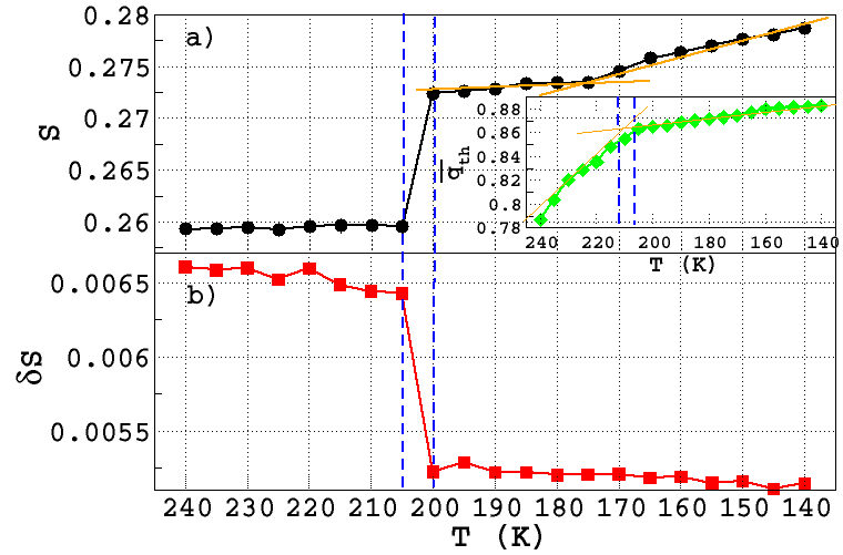
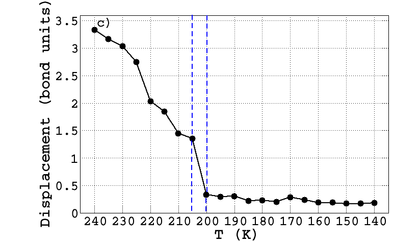
Figure 9: Evolution of $S$ (panel (a)) and $\delta S$ (panel (b)) during the water cooling protocol (see text). Panel (c) reports the corresponding evolution of the standard molecular displacement in a ns time in units of the bond length. The dashed vertical lines delimit the glass transition temperature ($T_{g}$) of the simulation. At $T=T_{g}$ the translational motions freeze.

In Fig. 9 we report the evolution of $S$ (panel (a)) and $\delta S$ (panel (b)) along the cooling protocol. Both OPs show a sudden, albeit small, change in correspondence with the vertical dashed blue lines. The sudden increase of $S$ indicates a sudden increase of the local order relative to that of the supercooled liquid. At the same time the sudden drop of $\delta S$ indicates reduced fluctuations of the local order relative to the supercooled liquid. The sharp variation of $S$ and $\delta S$ is associated to freezing of the translational motions in the system. This is illustrated in panel (c) of the same figure in which we report the standard displacement, i.e. the square root of the mean square displacement, of the molecules in a ns time, measured in units of the bond length (the nearest neighbor distance between the oxygen sites). While for $T\geq 205$ K the standard displacement is greater than $1$, indicating that each molecule on average moves by more than one bond length on a ns timescale, for $T\leq 200$ K the standard displacement drops well below $1$, indicating translational localization of the molecules. The freezing of the translational degrees of freedom marks the onset of the glass transition. The corresponding transition temperature, $T_{g}$, is located, in our simulation, in the interval bounded by the two dashed vertical lines. It is quite remarkable that a phenomenon usually associated with dynamics (viz. the freezing of translational diffusion) has a clear static counterpart, well captured by the two OPs based on the LOM. The static signature of the glass transition is also detected by the average tetrahedral order parameter $\bar{q}_{th}$ shown in the inset of Fig. 9, but in this case the effect is weaker as the transition is only signaled by a change of slope in the temperature variation of $\bar{q}_{th}$. Given that $\bar{q}_{th}$ weighs the tetrahedral order of the first shell of neighbors while the LOM focuses on the second shell of neighbors, we conclude that the second shell of neighbors provides a more sensitive gauge of the local order.

By further cooling the system below $T_{g}$ there is an evident change of slope in the increase of $S$ with temperature when $T$ is near $175$ K. No corresponding effect can be detected from the behavior of $\delta S$, which takes so small values to have lost sensitivity. This behavior is associated to the freezing of molecular rotations, as demonstrated in Fig. 10, which reports the time evolution over $1$ ns of $C(t)=\left<\mathbf{\mu}(0)\cdot\mathbf{\mu}(t)\right>$, the time autocorrelation function of the molecular dipole $\mathbf{\mu}$. The time decay of $C(t)$ is associated to rotational relaxation. In panel (a) of Fig. 10 one sees that $C(t)$ decays on the ns timescale when $T\geq 180$ K, whereas for $T\leq 170$ K no apparent relaxation can be detected. We infer that freezing of the rotational degrees of freedom occurs when T is near $175$ K in our simulation. Similar rotational freezing effects have been inferred in recent experiments shephard_molecular .

To get further insight on the relaxation processes associated to the rotational and translational motions of the molecules, we analyzed the changes of the hydrogen bond network occurring upon cooling by monitoring the corresponding changes in the distribution $P(n)$ of the $n-$member rings in the network. Here $n$ indicates the number of hydrogen bonds in a ring. We define hydrogen bonds with the Luzar-Chandler criterion luzar_hydrogen and follow King’s approach king for the ring statistics. We report $P(n)$ at different temperatures in Fig. 11. We see that $P(n)$ changes with temperature in the supercooled liquid (panel (a)) and also in the glass in the range of temperatures between $T_{g}$ and the temperature of rotational freezing (panel (b)), but below the latter no further changes in the topology of the network occur (panel (c)). As the temperature is lowered in the supercooled liquid longer member rings with $n\geq 8$ systematically disappear while the population of $6-$ and $7-$member rings increases, with a prevalence of the former. Longer member rings are associated to more disordered local environments with interstitial molecules populating the region between the first and the second shell of neighbors santra_local_2015 . Such configurations are typical of molecular environments with higher number density. As the temperature is lowered in the supercooled liquid at ambient pressure, this continuously transforms into a liquid with lower density. In the glass, at temperatures above rotational freezing, network relaxation still occurs, again with a reduction in the population of rings with $n\geq 8$, but this time this is accompanied by a reduction of the population of the $6-$fold rings and an increase of the population of the $7-$fold rings. This is because the only processes that can change the network topology in absence of diffusion are bond switches of the kind described in Ref. wooten_computer . In water these processes can be generated by rotations of the molecules. For instance, we found that in a frequent process of this kind two adjacent rings, a $6-$fold and an $8-$fold ring sharing a bond, transform into two adjacent $7-$fold rings sharing a bond. Finally, at temperatures below rotational freezing the network topology does not change in the timescale of the simulation. At these temperatures only local vibrational relaxation occurs. In a classical system vibrational disorder diminishes with temperature as reflected in the increase of $S$ at low temperature in Fig. 9 (a).

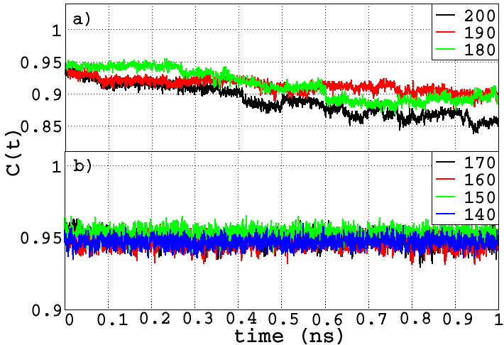
Figure 10: Time variation of the dipole autocorrelation function $C(t)$ in the temperature range $T\in[200,180]$ K (panel (a)) and in the temperature range $T\in[170,140]$ K (panel (b)). Each $C(t)$ curve is obtained by averaging 10 trajectories initiating at times separated by intervals of $100$ ps.

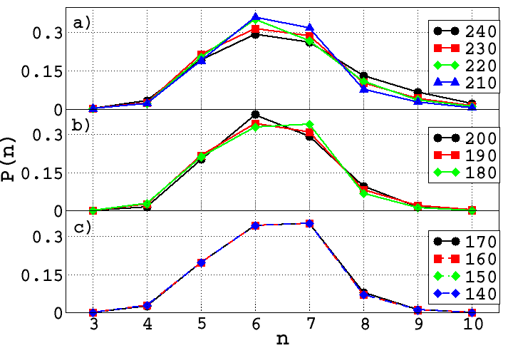
Figure 11: Ring distribution P(n) in the temperature range $T\in[240,210]$ K (panel (a)), in the temperature range $T\in[200,180]$ K (panel (b)), and in the temperature range $T\in[170,140]$ K (panel (c)).

VI Conclusions

We have introduced a local order metric (LOM) based on a simple measure of the optimal overlap between local configurations and reference patterns. In systems made of a repeated unit (atom or molecule) the LOM leads to the definition of two global order parameters, $S$ and its spread $\delta S$, which have higher resolving power than popular alternative OPs and are very useful to analyze structural changes in computer simulations, as shown by the examples in Section III, Section IV and Section V. The water examples show that the LOM can be used to measure the local order not only at atomic but also at molecular sites. Systems made by molecular units more complex than water could also be analyzed with this technique, while further generalizations could be envisioned for binary and multinary systems.

As defined, $S$ and $\delta S$ are not differentiable functions of the atomic (molecular) coordinates. This non-differentiability stems from two reasons: (1) the $M$ neighbors of a site may change abruptly in a simulation, and (2) the LOM depends on the permutations of pattern indices, which is a discrete variable. Thus $S$ and $\delta S$ could not be used as such to drive structural transformations in constrained molecular dynamics simulations. However, they could be used as collective variables in Monte Carlo simulations adopting enhanced sampling techniques, such as umbrella sampling torrie_nonphysical_1977 , metadynamics laio_escaping_2002 , replica exchange swendsen_replica_1986 etc..

- [1] P. J. Steinhardt, D. R. Nelson, and M. Ronchetti. Bond-orientational order in liquids and glasses. Phys. Rev. B, 28:784, 1983.
- [2] P. R. ten Wolde, M. J. Ruiz-Montero, and D. Frenkel. Numerical evidence for bcc ordering at the surface of a critical fcc nucleus. Phys. Rev. Lett., 75:2714, 1995.
- [3] W. Mickel, S. C. Kapfer, G. E. Schröder-Turk, and K. Mecke. Shortcomings of the bond orientational order parameter for the analysis of disordered particluate matter. J. Chem. Phys., 138:044501, 2013.
- [4] P. R. ten Wolde, M. J. Ruiz-Montero, and D. Frenkel. Numerical calculation of the rate of crystal nucleations in a lennard-jones system at moderate cooling. J. Chem. Phys., 104:9932, 1996.
- [5] P. R. ten Wolde and D. Frenkel. Homogeneous nucleation and the oswald step rule. Phys. Chem. Chem. Phys., 1:2191, 1999.
- [6] W. Lechner and C. Dellago. Accurate determination of crystal structures based on averaged local bond-order parameters. J. Chem. Phys., 129:114701, 2008.
- [7] L.M. Ghiringhelli, C. Valeriani, J. H. Los, E. J. Meijer, A. Fasolino, and D. Frenkel. State-of-the-art models for the phase diagram of carbon and diamond nucleation. Mol. Phys., 106:2011–2038, 2008.
- [8] T. Li, D. Donadio, G. Russo, and G. Galli. Homogeneous ice nucleation from supercooled water. Phys. Chem. Chem. Phys., 13:19807–19813, 2011.
- [9] T. A. Kesselring, E. Lascaris, G. Franzese, S. V. Buldyrev, H. J. Herrmann, and H. E. Stanley. Finite-size scaling investigation of the liquid-liquid critical point in ST2 water and its stability with respect to crystallization. J. Chem. Phys., 138:244506, 2013.
- [10] I. Volkov, M. Cieplak, J. Koplik, and J. R. Banavar. Molecular dynamics simulations of crystallization of hard spheres. Phys. Rev. E, 66:061401, 2002.
- [11] D. Moroni, P. R. ten Wolde, and P. G. Bolhuis. Interplay between structure and size in a critical crystal nucleus. Phys. Rev. Lett., 94:235703, 2005.
- [12] C. Desgranges and J. Delhommelle. Crystallization mechanism for supercooled liquid Xe at high pressure and temperature: hybrid monte carlo molecular simulations. Phys. Rev. B, 77:054201, 2008.
- [13] J. Russo, F. Romano, and H. Tanaka. New metastable form of ice and its role in the homogeneous crystallization of water. Nat. Mater., 13:733–739, 2014.
- [14] E. Sanz, C. Vega, J. R. Espinosa, R. Cabllero-Bernal, J. L. F. Abascal, and C. Valeriani. Homogeneous ice nucleation at moderate supercooling from molecular simulation. J. Am. Chem. Soc., 135:15008–15017, 2013.
- [15] P. J. Steinhardt, D. R. Nelson, and M. Ronchetti. Icosahedral bond orientational order in supercooled liquids. Phys. Rev. Lett., 47:1297, 1981.
- [16] E. Shiratani and M. Sasai. Growth and collapse of structural patterns in the hydrogen bond network in liquid water. J. Chem. Phys., 104:7671–7680, 1996.
- [17] E. Shiratani and M. Sasai. Molecular scale precursor of the liquid–liquid phase transition of water. J. Chem. Phys., 108:3264–3276, 1998.
- [18] M. J. Uttormark, M. O. Thompson, and P. Clancy. Kinetics of crystal dissolution for a stillinger-weber model of silicon. Phys. Rev. B, 47:15717, 1993.
- [19] P.-L. Chau and J. Hardwick. A new order parameter for tetrahedral configurations. Mol. Phys., 93:511–518, 1998.
- [20] J. R. Errington and P. G. Debenedetti. Relationship between structural order and the anomalies of liquid water. Nature, 409:318–321, 2001.
- [21] J. Russo and H. Tanaka. Understanding water’s anomalies with locally favoured structures. Nature Comm., 5:3556, 2013.
- [22] A. S. Keys, C. R. Iacovella, and S. C. Glotzer. Characterizing structure through shape matching and applications to self-assembly. Ann. Rev. Condens. Matt. Phys., 2:263–285, 2011.
- [23] C. R. Iacovella, A. S. Keys, M. A. Horsch, and S. C. Glotzer. Icosahedral packing of polymer-tethered nanospheres and stabilization of gyroid phase. Phys. Rev. E, 75:040801(R), 2007.
- [24] A. S. Keys, C. R. Iacovella, and S. C. Glotzer. Characterizing complex particle morphologies through shape matching: Descriptors, applications and algorithms. J. Comp. Phys., 230:6438–6463, 2011.
- [25] A. P. Bartók, R. Kondor, and G. Csányi. On representing chemical environments. Phys. Rev. B, 87:184115, 2013.
- [26] A. Haji-Akbari, M. Engel, A. S. Keys, X. Zheng, R. G. Petschek, P. Palffy-Muhoray, and S. C. Glotzer. Disorder, quasicrystalline and crystalline phases of densely packed tetrahedra. Nature, 462:773–777, 2009.
- [27] S. De, A. P. Bartók, G. Csányi, and M. Ceriotti. Comparing molecules and solids across structural and alchemical space. Phys. Chem. Chem. Phys., 18:13754–13769, 2016.
- [28] F. H. Stillinger and A. Rahman. Improved simulation of liquid water by molecular dynamics. J. Chem. Phys., 60:1545–1557, 1974.
- [29] V. Molinero and E. B. Moore. Water Modeled As an Intermediate Element between Carbon and Silicon†. J. Phys. Chem. B, 113:4008–4016, 2008.
- [30] J. L. F. Abascal and C. Vega. A general purpose model for the condensed phases of water: Tip4p/2005. J. Chem. Phys., 123:234505, 2005.
- [31] J. Chakrabarti and H. Löwen. Effect of confinement on charge-stabilized colloidal suspensions between two charged plates. Phys. Rev. E, 58:3400–3404, 1998.
- [32] F. A. Lindemann. Über die berechnung molekularer eigenfrequenzen. Phys. Z., 11:609–612, 1910.
- [33] Y. Da-Qi, M. Chen, and X.-J. Han. Structure analysis methods for crystalline solids and supercooled liquids. Phys. Rev. E, 75:051202, 2005.
- [34] D. Frenkel and B. Smit. Understanding molecular simulation: from algorithms to applications. Academic press, 2001.
- [35] A. K. Soper and M. A. Ricci. Structures of high-density and low-density water. Phys. Rev. Lett., 84:2881, 2000.
- [36] E. B. Moore, E de la Llave, K. Welke, D. A. Scherlis, and V. Molinero. Freezing, melting and structure of ice in a hydrophilic nanopore. Phys. Chem. Chem. Phys., 12:4124–4134, 2010.
- [37] E. B. Moore and V. Molinero. Is it cubic? Ice crystallization from deeply supercooled water. Phys. Chem. Chem. Phys., 13:20008–20016, 2011.
- [38] A. H. Nguyen and V. Molinero. Identification of clathrate hydrates, hexagonal ice, cubic ice, and liquid water in simulations: the chill+ algorithm. J. Phys. Chem. B, 119:9369–9376, 2015.
- [39] E. Mayer. New method for vitrifying water and other liquids by rapid cooling of their aerosols. J. Appl. Phys., 58:663, 1985.
- [40] J. Wong, D. A. Jahn, and N. Giovanbattista. Pressure-induced transformations in glassy water: A computer simulation study using the model. J. Chem. Phys., 143:074501, 2015.
- [41] J. J. Shephard and C. G. Salzmann. Molecular reorientation dynamics govern the glass transitions of the amorphous ices. J. Phys. Chem. Lett., 7:2281–2285, 2016.
- [42] A. Luzar and D. Chandler. Hydrogen-bond kinetics in liquid water. Nature, 379:55–57, 1996.
- [43] S. V. King. Ring configurations in a random network model of vitreous silica. Nature, 213:1112–1113, 1967.
- [44] B. Santra, R. A. DiStasio Jr., F. Martelli, and R. Car. Local structure analysis in ab initio liquid water. Mol. Phys., 113:2829–2841, 2015.
- [45] F. Wooten, K. Winer, and D. Weaire. Computer generation of structural models of amorphous si and ge. Phys. Rev. Lett., 54:1392–1395, 1985.
- [46] G. M. Torrie and J. P. Valleau. Nonphysical sampling distribution in monte carlo free-energy estimation: Umbrella sampling. J. Comp. Phys., 23:187–199, 1977.
- [47] A. Laio and M. Parrinello. Escaping free-energy minima. Proc. Natl. Acad. Sci., 99:12562–12566, 2002.
- [48] R. H. Swendsen and J.-S. Wang. Replica monte carlo simulation of spin-glasses. Phys. Rev. Lett., 57:2607, 1986.