The polaron paradigm: a dual coupling effective band model

Abstract

Non-diagonal couplings to a bosonic bath completely change polaronic dynamics, from the usual diagonally-coupled paradigm of smoothly-varying properties. We study, using analytic and numerical methods, a model having both diagonal Holstein and non-diagonal Su-Schrieffer-Heeger (SSH) couplings. The critical coupling found previously in the pure SSH model, at which the $k=0$ effective mass diverges, now becomes a transition line in the coupling constant plane - the form of the line depends on the adiabaticity parameter. Detailed results are given for the quasiparticle and ground state properties, over a wide range of couplings and adiabaticity ratios. The new paradigm involves a destabilization, at the transition line, of the simple Holstein polaron to one with a finite ground-state momentum, but with everywhere a continuously evolving band shape. No ’self-trapping transition’ exists in any of these models. The physics may be understood entirely in terms of competition between different hopping terms in a simple renormalized effective band theory. The possibility of further transitions is suggested by the results.

I Introduction

An electron moving in a solid (ordered or otherwise) polarizes its surroundings, and dresses itself with bosonic excitations which include electronic spin and charge fluctuations, electronic orbital fluctuations, and phonons. The result is a polaron; the best-known example is an electron dressed by a combination of optical and acoustic phonons. The phonon-dressed polaron is of enduring interest for two main reasons:

(i) Polarons are believed to play a key role in determining the physics of many materials; and

(ii) It provides a target for any theory of quasiparticles which tries to span the weak, intermediate, and strong coupling regimes. This has given the subject an interesting history (briefly described in section II), closely connected to many of the important developments in many-body physics and quantum field theory.

For most of this history, attention has focused on a specific kind of ”diagonal” coupling between the density of electrons (this is a diagonal operator in a real space formulation) and phonon displacements; the latter can be local or longer-range, as reviewed in section II. Such models are now well understood, and have led to a ”polaron paradigm” in which diagonal interactions, no matter what their form, do not lead to any kind of sharp transition in the polaron properties as the coupling strength is increased (eg., the effective mass increases smoothly with coupling, up to infinite coupling strength).

However one may also have non-diagonal couplings to the bath, only acting when the particle hops between sites (which in the continuum limit couple to the particle momentum). We now know that such couplings lead to results very different from the classical polaron paradigm. This was first shown in Ref. PRL, for a specific model with a non-diagonal coupling (the SSH model); a sharp transition was found between the behavior at weak coupling and that at strong coupling. As we shall see here, this transition persists even when we add diagonal interactions to the non-diagonal ones.

These results appear to be rather general, indicating that the old polaron paradigm needs to be replaced by a rather different one incorporating the interplay between diagonal and non-diagonal couplings. This is what we do in this paper. The results are not just of theoretical interest - they will force a substantial re-evaluation of our picture of polarons in many physical systems.

The plan of the paper is as follows. Section II discusses models containing both diagonal and non-diagonal terms, and briefly reviews previous work. Section III describes our method, the ’Bold Diagrammatic Monte Carlo’ (BDMC) and the momentum average (MA) approximation. The former method is also discussed in Appendix A, which is an integral part of the paper. Sections IV and V give the main results; Section IV discusses the results when only non-diagonal SSH terms are present, highlighting the transition in the polaronic properties. Section V adds diagonal terms, and shows how the transition is influenced by these terms. Section VI summarizes the new picture of the polaron that comes out of these results, in the form of an effective band theory leading to a new kind of polaron paradigm - readers looking for a quick summary should go to this section, which also discusses experimental applications.

II The model

We would like to study a model which brings out the main features of both diagonal and non-diagonal couplings without being too complicated. In this section we first develop the model, and then discuss a few simple key features it possesses, at the same time recalling some of the main results found over the years.

II.1 Derivation of the dual coupling model

We begin by formulating the dual coupling model in a fairly general way. In a site basis we start from a Hamiltonian

$$\hat{\mathcal{H}}_{o}\;=\;-\sum_{ij}t_{ij}(\{b_{\lambda}\})c_{i}^{\dagger}c_{j} + \sum_{i}\epsilon_{i}(\{b_{\lambda}\})c_{i}^{\dagger}c_{i}$$ (1)

$$+ \sum_{\lambda}\omega_{\lambda}b_{\lambda}^{\dagger}b_{\lambda}$$

describing the hopping, with amplitude $t_{ij}$, of a particle between sites $i$ and $j$ of a lattice, in the presence of a bosonic bath having a single branch of excitations of frequency $\omega_{\lambda}$ (here, $\lambda$ labels the quantum numbers of the bosons; for example, we can choose $\lambda=\{{\bf q},\mu\}$, where ${\bf q}$ is a momentum and $\mu$ a polarization; or we can choose $\lambda=\{i,\mu\}$, with $i$ a site index again). Both the on-site energy $\epsilon_{i}$ and the hopping matrix element $t_{ij}$ are modulated by (i.e., are functionals of) the boson variables $b_{\lambda},b_{\lambda}^{\dagger}$. If we are dealing with lattice phonons, the modulation is through the site displacement operators $\hat{x}_{\lambda}=\sqrt{\hbar\over 2M\omega_{\lambda}}\left(b_{\lambda}+b_{\lambda}^{\dagger}\right)$, where $M$ is the ionic mass. This generates the diagonal couplings (modulations of $\epsilon_{i}$) and non-diagonal couplings (modulations of $t_{ij}$).

The form of (1) is quite general - the lattice may take any form (ordered or disordered), as may the various coupling terms. To say more we must specify how $\epsilon_{i}$ and $t_{ij}$ depend on the bosonic variables. This dependence can take many forms for different physical systems. In what follows, we will assume that we are dealing with a periodic crystalline lattice, and that the bosons in questions are lattice phonons; crystal momentum is then a good quantum number.

Let us expand the Hamiltonian (1) in terms of the phonon variables $\{b_{\lambda}\}$. Then the diagonal interaction terms are produced by expanding the on-site energy:

$$\epsilon_{i}=\epsilon_{o} + \sum_{\lambda}U^{(1)}_{i}(\lambda)(b_{\lambda}+b_{\lambda}^{\dagger})$$ (2)

$$+ \sum_{\lambda\lambda^{\prime}}U^{(2)}_{i}(\lambda,\lambda^{\prime})(b_{\lambda}+b_{\lambda}^{\dagger})(b_{\lambda^{\prime}}+b_{\lambda^{\prime}}^{\dagger})+...$$

where $U^{(1)}_{i}(\lambda)$ is the 1-phonon diagonal coupling, $U^{(2)}_{i}(\lambda,\lambda^{\prime})$ the 2-phonon diagonal coupling, and so on. This diagonal term arises simply from the polarization of the background lattice by the particle - for electrons, it is essentially a Coulomb interaction effect.

The non-diagonal couplings are produced by expanding $t_{ij}(\{b_{\lambda}\})$ in phonon variables. This is more subtle, since the hopping matrix element arises from electron tunneling, and so depends exponentially on the phonon displacement. Often this dependence is written as

$$t_{ij}(\{b_{\lambda}\})=t_{o}\exp\left[-\sum_{\lambda}{V_{ij}(\lambda)\over\omega_{\lambda}}(b_{\lambda}+b_{\lambda}^{\dagger})\right]$$ (3)

where $V_{ij}(\lambda)$ has the dimension of energy; but this form generates only one part of the multi-phonon interaction terms (which can also appear directly in the exponent). However since we are only interested in the linear term, we expand (3) to linear order in phonon variables, so that

$$t_{ij}(\{b_{\lambda}\})=t_{o}\left[1-\sum_{\lambda}{V_{ij}(\lambda)\over\omega_{\lambda}}(b_{\lambda}+b_{\lambda}^{\dagger})\right]$$ (4)

The physical meaning of this ’Peierls’ term is obvious from the derivation - the phonons modulate the distance between the lattice ions, and this modulates the tunneling amplitude of the electron between sites. As we shall see, the effective range of the $t_{ij}$, once it is renormalized by the coupling to phonons, can be significantly greater than a single lattice spacing.

In this paper we will deal exclusively with ordered lattices. We then Fourier transform the starting Hamiltonian (1); and as further restrictions, we will (i) keep only the linear coupling to phonons; (ii) assume a single optical phonon branch, with polarization index suppressed and frequency $\omega_{\bf q}$; and (iii) assume the lattice has no impurities, defects, surfaces, or other inhomogeneities that break translational invariance. The Hamiltonian describing such problems then has the general structure:

$$\hat{\mathcal{H}} = \sum_{k}\epsilon_{k}c_{k}^{\dagger}c_{k}+\sum_{q}\omega_{q}b_{q}^{\dagger}b_{q}$$ (5)

$$+ \frac{1}{\sqrt{N}}\sum_{k,q}V(k,q)\;c_{k-q}^{\dagger}c_{k}\big{(}b_{q}^{\dagger}+b_{-q}\big{)},$$

where we suppress the electronic spin variable. Here $V(k,q)$ is the sum of the Fourier-transformed diagonal and non-diagonal terms, $c_{k}^{\dagger},b_{q}^{\dagger}$ are electron and phonon creation operators, $k$ is the electron momentum and momentum sums are over the first Brillouin zone. We assume $N$ lattice sites and let $N\rightarrow\infty$. The elimination of both acoustic phonons and higher-order phonon couplings restricts the applicability of (5) in the real world. In section VI we return to these approximations and their consequences.

Splitting $V(k,q)$ into its diagonal and non-diagonal parts, we have

$$g({k},{q})=g_{1}({q})+g_{2}({k},{q})$$ (6)

where the diagonal coupling $g_{1}({q})$ depends only on the phonon momentum ${q}$, while the non-diagonal coupling $g_{2}({k,q})$ depends explicitly on the particle momentum ${k}$.

The Dual ”H/SSH” model: So far these results are purely formal. In most of the rest of this paper we wish to obtain explicit results for the polaron properties in a model which combines two specific forms for the diagonal and non-diagonal couplings. We therefore consider a 1-dimensional chain with lattice constant $a_{o}=1$, and a bare hopping term $t_{ij}\rightarrow t_{o}\delta_{i\pm 1,j}$, i.e., constant nearest-neighbor hopping only. We choose the phonons to be a set of Einstein phonons of frequency $\Omega_{o}$. The non-interacting part of ${\cal H}$ in (5) is then

$${\cal H}_{o}\;=\;-2t_{o}\sum_{k}\cos k\;c_{k}^{\dagger}c_{k}+\sum_{q}\Omega_{o}b_{q}^{\dagger}b_{q}$$ (7)

giving two characteristic energy scales, $t_{o}$ and $\Omega_{o}$.

For the diagonal electron-phonon coupling we use a simple on-site Holstein coupling,Holstein so that

$$g_{1}(q)\rightarrow g_{o}$$ (8)

with no dependence on momentum at all. For the non-diagonal coupling we use the so-called Su-Schrieffer-Heeger (SSH) form,PhysRevLett.42.1698 ; RevModPhys.60.781 ; BLB1 ; BLB2 which describes the modulation of the hopping term, viz.,

$$t_{i,i+1}\rightarrow\;t_{o}-\alpha_{o}(x_{i+1}-x_{i})$$ (9)

which in momentum space gives a coupling

$$g_{2}(k,q)=\frac{2i}{\sqrt{N}}\alpha_{o}\left[\sin(k-q)-\sin k\right]$$ (10)

and we have introduced 2 new energy scales, $g_{o}$ and $\alpha_{o}$.

We see that if we scale everything in terms of $t_{o}$, there are 3 independent parameters in this ”H/SSH” model. The adiabaticity parameter is:

$$\Lambda_{o}=\Omega_{o}/(4t_{o}),$$ (11)

so that when $\Lambda_{o}\ll 1$, the phonon dynamics is considered as slow (and the electron dynamics is fast). One can also define dimensionless parameters $g_{o}/t_{o}$ and $2\alpha_{o}/t_{o}$, with dimensionless ratio $2\alpha_{o}/g_{o}$. However, a better understanding of the physics is obtained by defining

$$\lambda_{H} = {g_{o}^{2}\over 2t_{o}\Omega_{o}}\;\;\;\;\;\;(diagonal)$$ (12)

$$\lambda_{SSH} = {2\alpha_{o}^{2}\over t_{o}\Omega_{o}}\;\;\;\;\;\;(non-diagonal)$$ (13)

whose ratio is now $(2\alpha_{o}/g_{o})^{2}$. Along with $\Lambda_{o}$, these dimensionless parameters determine the behavior of this model at zero temperature.

This is the simplest model one can look at for a polaronic system with both diagonal and non-diagonal couplings. It is something of a toy model and it ignores acoustic phonons. Nevertheless it is good enough to reveal the main features of an entirely new behavior for the polaron, one quite different from the polaronic paradigm described above. How much these general features will persist in more general models is a question we address at the end of the paper.

II.2 Basic features of the model

A great deal is known about the effect of the coupling $g_{1}$ on polaron dynamics, much less about $g_{2}$, and still less about the effect of a combination of the two. The main results that have so far been established are as follows.

(i) Diagonal terms: As noted above, many models with different diagonal couplings have been studied. The most famous examples are the Holstein modelHolstein (where, as just noted, $g_{1}({q})\rightarrow g_{o}$, a constant) and the Fröhlich model, Frohlich where the form of $g_{1}({q})$ depends on the spatial dimension and on whether we deal with a lattice or a continuous medium model). Other examples include the Rashba-Pekar model,RaPe breathing-mode (BM) models,bmo and various models with displacement potential coupling.Mahan A variety of theoretical methods to study them were developed in the period from 1940 to 1970, including perturbation expansions in the interaction, lang:firsov:63 semiclassical approximations landau33 ; Toyozawa , and path integral techniques.Feynman The main aim was to understand the behavior of the polaron as the strength of the diagonal coupling $g_{1}({q})$ was increased. Indeed, the problem was (and still is) regarded as providing a key test of non-perturbative methods, and thus of interest well beyond solid-state physics. More recently, other methods have been developed, notably the Dynamical Mean-Field Theory (DMFT)DMFT and the Momentum Average (MA) approximations.MA ; MAh ; MAq The predictions of all of these methods can now be checked by a wide variety of numerical techniques, including exact diagonalization, variational methods, various types of Quantum Monte Carlo simulations, and in one dimension, by Density Matrix Renormalization Group (DMRG) methods. The literature on all this is now enormous.reviews

These diagonal models all have certain broad features in common. For weak coupling, there is typically very little phonon dressing, and the polaron properties are only slightly renormalized. This weak coupling regime is sometimes called the large polaron regime (although that term may be more appropriate for continuous models). As the coupling is increased, there is a crossover to the small polaron regime, where a robust polarization cloud is formed, and the electronic properties are strongly renormalized. The effective mass then increases rapidly with coupling (eg., exponentially fast in the Holstein model). For a long time there was significant confusion over the idea that in this strong-coupling regime the polaron might become self-trapped (i.e. localized), although it is now clear that such self-trapping is impossible in a clean system for any finite coupling. Disorder in real systems can of course localize polarons, particularly when they are heavy; but this is a different effect. Another related, and long-standing controversy, was over whether there is a sharp transition or a smooth crossover between the two regimes. This question was settled by the work of Gerlach and Löwen RevModPhys.63.63 who showed that for diagonal models having gapped bosonic modes, sharp transitions in the polaronic properties are impossible; all physical quantities must vary smoothly with coupling strength. We note that the so-called ’self-trapping transition’, which has in the past often been asserted to exist at some finite value of the coupling, is actually typically an artefact of numerical approximations, arising when the effective bandwidth is decreasing rapidly with increasing coupling constant.

Thus we see that from all of this work a general consensus has emerged for the diagonal coupling model, both on the essential physics and on the detailed quantitative picture. This is the ”polaron paradigm”; as conventionally understood, it involves a smooth crossover between weak and strong coupling, and between large and small polaron behavior, with no sharp transition of any kind; and for a clean system, no ”self-trapping” or localization of the polaron on any particular site.

(ii) Non-Diagonal Terms: Much less work has been done on the non-diagonally coupled model, and most of this has been in the context of applications to systems like polyacetylene (the SSH model PhysRevLett.42.1698 ; RevModPhys.60.781 ; RiceMele ) and other polyacenes, polyacene ; rubrene as well as excimers, excimer MX chains,MX and the cuprate superconductors.nagaosa04 Most theoretical studies of the single polaron in such models have been fairly recent, and we can separate them into two categories.

First, several studies have argued that in dual coupling models, having both diagonal and non-diagonal interactions, one can discern a ’self-trapping’ transition line in the 2-dimensional plane of the 2 couplings. Evidence cited for this has typically come from variational analyses, using either a Toyozawa ansatz sun09 or a ’global-local’ ansatz PhysRevB.79.165105 . There are also perturbative analyses PhysRevB.56.4484 ; PhysRevB.66.012303 ; Mars , supplemented by exact diagonalization studies PhysRevB.56.4484 on very small (4-site) lattices, that have claimed evidence for a crossover (not a transition) between large and small polaron regimes as a function of a non-diagonal SSH coupling (note that Refs. PhysRevB.66.012303, and Mars, have non-diagonal coupling to acoustic rather than optical phonons).

Second, a few papers have looked at the entanglement between the polaronic particle and the phonon bath as a function of the coupling constants - this was first done for the Holstein model,zhao04 and then for the SSH model.stojan08 In the pure Holstein model the entanglement increases smoothly during the crossover between the large and small polaron limits (this is described as a cliff-like transition by Zhao et al., zhao04 but in fact their results show only a smooth change in the entanglement). Stojanović and Vanević then found, in the SSH model, a non-analyticity in the entanglement as a function of the SSH coupling,stojan08 but they then argued that this did not signal any kind of transition in the polaronic properties (in particular, no change in the ground state), but rather a loss of coherence of the polaron.

In sections IV and V we will demonstrate that the physics is very different from that proposed by these earlier analyses. In fact there really is a sharp transition line in the dual coupling parameter plane, but it has nothing to do with any kind of ’phase transition’ or even a crossover between large and small polarons, or to a self-trapped state; nor is it in the same part of the parameter space as the transitions claimed in the previous work. Instead, it is associated with a change in the ground state, coming from a continuous evolution of the band structure as a function of the non-diagonal coupling. The $k=0$ polaron effective mass actually diverges along the transition line - but this is simply because of the shift of the ground state momentum; the bandwidth is finite even at the transition. Thus, the polaron is mobile everywhere in the parameter plane, even on the critical line. The crossover between large and small polarons turns out to be entirely associated with the diagonal part of the coupling - the non-diagonal coupling plays no role in this. Sections IV-V gives full details of the results, and section VI describes the new picture that emerges from them.

III Methods: Perturbative and Numerical

One reason we are confident in the accuracy of the results discussed herein is that we have been able to benchmark them against results found with the extremely powerful diagrammatic Monte Carlo (DMC) method invented by Prokof’ev, Svistunov and Tupitsyn.prokofev-1998-87 In the current work we have augmented this method with an improved version, the Bold Diagrammatic Monte Carlo (BDMC) method, and we have also used the much faster Momentum Averaging (MA) approximation. In what follows we describe how they are applied to the present problem - technical details for the BDMC method are relegated to the Appendix. We also say a little about perturbation theory - this turns out to work well only in the extreme anti-adiabatic regime when $\Lambda_{o}\gg 1$.

In Ref. PRL, , results were reported for the SSH model using the above methods and also the Limited Phonon Basis Exact Diagonalization (LPBED) method.PhysRevB.80.195104 The agreement between the LPBED, DMC, BDMC and MA results was found to be excellent, and we expect this to also be true for the present dual-coupling model because all these methods also work well for the Holstein model.

III.1 Perturbation theory

For perturbative work, we write $\Sigma(k,\omega)=\sum_{l}\Sigma_{l}(k,\omega)$, where $\Sigma_{l}(k,\omega)$ is the sum of all self-energy graphs containing $l$ internal boson lines. Both the Rayleigh-Schrodinger and Wigner-Brillouin versions of perturbation theory are then applied. In Rayleigh-Schrödinger (RS) perturbation theory it is well-known rspt_frolich that for polaron models with Einstein phonons and $\Omega_{o}<4t_{o}$, the first order contribution to $E_{k}$ exhibits an unphysical maximum at some momentum $k_{m}>0$, and an unphysical divergent energy at larger momenta. Because of this, we can only calculate the ground state energy and the effective mass if the ground-state is located at $k=0$. At second order, the unphysical maximum is eliminated and so is the divergent negative ground state energy, but for $\Omega_{o}<4t_{o}$ one finds instead a positive divergent energy at larger momentum.

In Wigner-Brillouin (WB) perturbation theory, where the polaron energy is approximated using the implicit equation $E_{k}=\epsilon_{k}+\mbox{Re}\Sigma(k,E_{k})$, no singular values for $E_{k}$ are found anywhere in the Brillouin zone. WB is also useful as a consistency check for any numerical code: if electron lines are not dressed, and only contributions of up to two phonon lines are allowed, the resulting self-energy must converge to $\Sigma_{2}(k,\omega)$. Since the polaron energy $E_{k}$ is the lowest pole of the Green’s function $G(k,\omega)=[\omega-\epsilon_{k}-\Sigma(k,\omega)]^{-1}$, with these restrictions any numerical results must coincide with WB.

III.2 Momentum Average (MA) approximation

The MA technique is a non-perturbative approximation which has been applied successfully to a number of polaron problems. MA ; MAh ; MAq ; PhysRevB.82.085116 ; MAca It sums all diagrams in the self-energy expansion, up to exponentially small contributions which are discarded. The MA self-energy is then expressed in closed form as a continued fraction, and evaluates this very efficiently. MA can be systematically improvedMAh so that its convergence can be assessed. It can also be cast in variational terms, as keeping contributions only from processes consistent with a certain structure of the phonon cloud. In its simplest, original formulation (already surprisingly accurate for the Holstein model), the phonon cloud can be arbitrarily far from the electron and contain arbitrarily many phonons, but its size is limited to one site.MAh ; MAvar For the Edwards modelEdwards – another model describing boson-modulated hopping – it was shown that to correctly describe the polaron dynamics, the minimum extent of the cloud is over three adjacent sites (again, an arbitrary number of bosons is allowed at each site, and the particle can be arbitrarily far away from the cloud).PhysRevB.82.085116

The MA results presented here have been generated using a straightforward generalization of the work in Ref. PhysRevB.82.085116, . On general grounds, we expect it to be accurate if $\Lambda_{o}$ is not too small; if phonons are energetically expensive, having them spread over many sites becomes very unlikely. Of course, one can generalize MA to allow for more extended clouds, but the calculations become rather cumbersome. As shown below, the MA results produced here are quantitatively quite accurate as long as $\Lambda_{o}\geq 0.1$ or so. Note that we are using here what is technically called a MA⁽⁰⁾ method, which does not allow additional phonons to exist away from the polaron cloud. As a result, it cannot describe the polaron $+$ one-phonon continuum, expected to appear at an energy $\Omega_{o}$ above the polaron ground-state energy. MA properly captures this continuum for MA⁽¹⁾ or higher level approximations, which include these states amongst those kept in the variational space.MAh However, here we are concerned with the polaron band which lies below this continuum, and this MA version is already sufficient to describe it accurately, and to allow us to efficiently evaluate various trends.

III.3 Bold Diagrammatic Monte Carlo (BDMC)

The BDMC method PhysRevLett.99.250201 ; PhysRevB.77.020408 ; PhysRevB.77.125101 is an elaboration of the earlier Diagrammatic Monte Carlo (DMC) algorithm.prokofev-1998-87 Both belong to a category of unbiased computational methods, in which no assumptions are made about the solution or the type of diagrams that contribute most to the final answer. Instead, all the diagrams are summed using stochastic sampling, and the result is exact within the statistical error bars. The DMC method was further developed to study the Fröhlich polaron, PhysRevLett.81.2514 ; PhysRevB.62.6317 the Holstein polaronMacridin2003 and the spin polaron, PhysRevB.64.033101 amongst others. Recently, it was also extended to many-polaron problems.Mnew

The method is formulated in imaginary time, where all diagrams are real functions of the internal lines. For diagonal coupling models, with $V(k,q)=g_{1}(q)$, this removes any sign problem because in any self-energy diagram all emitted bosons are reabsorbed, so the vertices contribute a positive factor $g_{1}(q)g_{1}(-q)=|g_{1}(q)|^{2}>0$ irrespective of the topology of the diagram. In this case their sum is convergent, and success is guaranteed.

For models with non-diagonal couplings $g_{2}(k,q)$, however, this is no longer necessarily true. Hermiticity of the Hamiltonian guarantees that $g_{2}(k^{\prime},-q)=g_{2}^{*}(k^{\prime}+q,q)$, so if we consider the vertex product $g_{2}(k,q)g_{2}(k^{\prime},-q)$ for a phonon line with momentum $q$, its contribution is positive only if $k^{\prime}=k-q$, i.e., if this phonon line is not crossed by other phonon lines. At first sight, it looks as if these contributions are complex, not real; however, this is not the case because of symmetries. For example, for our dual-coupling H/SSH model, a purely imaginary contribution comes from diagrams where an odd number of phonon lines are either emitted by a Holstein process and absorbed by a SSH process, or vice-versa. One can check that the contribution of such a diagram is canceled by that of its time-reversed pair. Only diagrams with an even number of both Holstein and of SSH vertexes survive. These have real expressions, but diagrams with crossed phonon lines can now have either sign.

Thus we see that for $\alpha_{o}\neq 0$, our model has a sign problem. It is not a severe problem because at least all the non-crossed diagrams are positive, but it makes it desirable to perform partial summations of diagrams, which may further mitigate it. This idea gave rise to the BDMC algorithm, in which free propagator lines are replaced by “bold” lines which already include some of the self-energy contributions. This is done in an iterative fashion, with proper care to avoid double counting of diagrams.

To the best of our knowledge, our results reported in Ref. PRL, and here are the first BDMC results for a single polaron problem; in the Appendix we explain in more detail how these calculations were done.

IV Results: Holstein and SSH models

Before looking at the results when we have both couplings in the system, we examine each model separately. The physics of the diagonal Holstein model is well-known - our purpose in discussing it here is to demonstrate the accuracy of the methods. We then examine the SSH model using the same methods, and discuss the physics around the critical coupling where the transition takes place, and the physical mechanism which causes the transition.

IV.1 Pure Holstein model

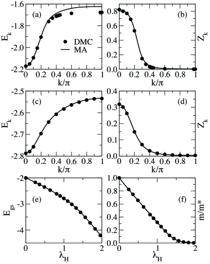
Figure 1: Results for the 1D Holstein model, using DMC (symbols) and MA (lines). (a) Polaron energy $E_{k}$ and (b) its $qp$ weight $Z_{k}$, for $\lambda_{H}=0.25$; (c) polaron energy $E_{k}$ and (d) its $qp$ weight $Z_{k}$, for $\lambda_{H}=1.0$; (e) polaron ground-state energy $E_{gs}$ and (f) its inverse effective mass $m/m^{*}(k=0)$ vs. $\lambda_{H}$ at $k=0$. In all cases, $t_{o}=1$, $\Lambda_{o}\equiv\Omega_{o}/(4t_{o})=0.125$, and $\lambda_{SSH}=0$. DMC data are from Ref. Macridin2003, .

The standard properties of interest in the diagonally-coupled models like the Holstein model are (i) the polaronic properties, notably the quasiparticle dispersion relationship $E_{k}$ and the related quasiparticle weight $Z_{k}$, along with the polaronic effective mass $m^{*}$, as functions of both quasiparticle momentum and electron-phonon coupling strength; and (ii) the energy $E_{gs}$ of the polaronic ground state, i.e., the minimum quasiparticle energy, as a function of the coupling strength.

In what follows we describe one set of results for this model, to see how well the different numerical methods work in this well-understood case; this also serves to illustrate the main features of the standard polaron paradigm. Both MA and DMC data are given (there is no difference between DMC and BDMC results; BDMC is simply computationally more efficient).

Fig. 1 shows different quasiparticle quantities for the Holstein polaron. To be specific, we assume an adiabacity parameter $\Lambda_{o}=0.125$. Panels (a) and (b) show the polaron dispersion $E_{k}$ and quasiparticle ($qp$) weight $Z_{k}$ in half of the Brillouin zone, in the weak coupling regime (for $\lambda_{H}=0.25$). Here the MA results overestimate the bandwidth – as already discussed above, this is because this is a MA⁽⁰⁾-type method, which does not properly account for the location of the polaron+one-phonon continuum (higher level MA approximations fix this problemMAh ). As the Holstein coupling $\lambda_{H}$ increases, the polaron bandwidth decreases below $\Omega_{o}$ and the agreement becomes excellent everywhere, as shown in panels (c) and (d) for $\lambda_{H}=1$. The agreement improves even further for larger $\lambda_{H}$ (not shown), since any flavor of MA becomes exact MA in the limit $\lambda_{H}\rightarrow\infty$. The decreasing bandwidth corresponds here to an increasing effective mass $m^{*}(k)$, where we define this mass in the usual way as

$$m^{*}(k)=\bigg{[}\frac{\partial^{2}E_{k}}{\partial k^{2}}\bigg{]}^{-1}$$ (14)

The inverse of this effective mass is shown in (f) for $k=0$. We notice how rapidly the bandwidth and corresponding inverse effective mass decrease for $\lambda_{H}>1$ (thus, for $\lambda_{H}=1$, we see from (c) that the bandwidth $\sim 0.25t_{o}$, whereas for $\lambda_{H}=2$, it is $\sim 0.005t_{o}$). However, we also note that there is no sudden collapse or discontinuity of any kind in the effective mass as a function of $\lambda_{H}$.

In panel (e) we look at the ground state energy, and confirm that the MA and DMC methods agree with each other; ground-state properties are described accurately by MA for all couplings $\lambda_{H}$. No qualitative changes are expected for these properties, if $\Lambda_{o}$ is increased. Note that the accuracy of the MA results is improved, especially at intermediary couplings, over that shown in Fig. 10 of Ref. MA, . This is because here we allow for a polaron cloud extending over up to three adjacent sites, whereas there we only considered a one-site cloud.

These results illustrate well the standard polaron paradigm. As coupling increases, the bandwidth decreases monotonically with a corresponding increase in the effective mass. The basic shape of the dispersion relation is unchanged, with the usual monotonic increase of energy with momentum, qualitatively similar to that of the bare particle. All properties vary smoothly with $\lambda_{H}$; as expected, there is no trace of any kind of transition or non-analyticity in either the quasiparticle properties or the energy,RevModPhys.63.63 as functions of either the coupling strength or the momentum. Although details will change if we change the momentum dependence of the coupling $g(q)$, the polaron behavior is qualitatively similar.

IV.2 Pure SSH model

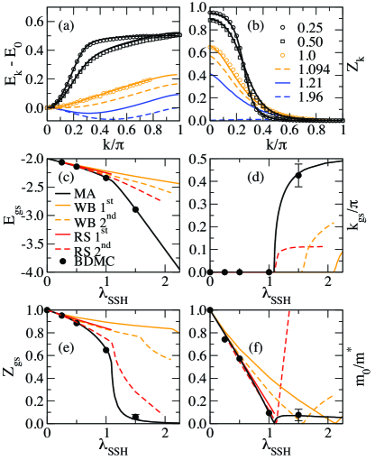
Figure 2: (color online) Results for the 1D SSH model with $\Lambda_{o}\equiv\Omega_{o}/(4t_{o})=0.125$ from BDMC, MA, and 1^st and 2^nd order RS and WB perturbation theory. (a) Shifted polaron energy $E_{k}-E_{0}$ and (b) its $qp$ weight $Z_{k}$, for $\lambda_{SSH}=0.25,0.5,1,1.094,1.21,1.96$, with BDMC (symbols) and MA (lines). (c) Polaron ground-state energy $E_{gs}$, (d) the ground-state momentum $k_{gs}$, (e) the ground-state $qp$ weight $Z_{gs}$ and (f) the inverse effective mass $m/m^{*}(k=k_{gs})$, all as functions of $\lambda_{SSH}$. Panels (c)-(f) share the same colour code described in the legend of panel (c). For BDMC results, error bars are shown only when they are larger than the size of the symbols. In all cases, $t_{o}=1$ and $\lambda_{H}=0$.

In the SSH model we need to look at the quasiparticle properties a little differently. This is because the key feature is the sharp transition which we find at a critical coupling $\lambda_{SSH}^{*}(\Lambda_{o})$; this transition changes the way we must characterize the polaron quasiparticle. In addition to the usual quantities $E_{k},Z_{k}$, and $m^{*}$, we also need to look at the ground state momentum $k_{gs}$, which changes rather quickly once $\lambda_{SSH}>\lambda_{SSH}^{*}$; and the ground state energy, which of course now depends on $k_{gs}$.

(i) Numerical results: To see what happens, we begin in Fig. 2 with SSH results for the same value $\Lambda_{o}=0.125$ as above, so we can directly compare with the Holstein result of Fig. 1. Panels (a) and (b) show the polaron energy $E_{k}$ (shifted so that all curves start at zero) and $qp$ weight $Z_{k}$. For weak couplings, the curves look rather similar to those of the Holstein model – the dispersion is monotonic and it flattens out just below the continuum (whose energy is again slightly overestimated by MA). However, for medium and strong couplings the results are very different. The dispersion does not simply become flatter; instead it changes its shape so that the ground-state is no longer at $k_{gs}=0$. In (c) and (d) we see clearly that the transition involves a non-analytic dependence of both the ground-state energy $E_{gs}(k_{gs})$ and the ground-state momentum $k_{gs}$ on the coupling constant, with discontinuities in all derivatives of these quantities with respect to $\lambda_{SSH}$ at $\lambda_{SSH}=\lambda_{SSH}^{*}$. Notice from (c) and (d) that, even though perturbation theory gives a very poor description of $E_{gs}$ and $k_{gs}$ as functions of $\lambda_{SSH}$, nevertheless a 2^nd-order Rayleigh-Schrodinger calculation does capture the correct position of the singularity.

This pattern is repeated in calculations of $Z_{k}$ and the effective mass $m^{*}(k)$ as functions of $\lambda_{SSH}$, provided we evaluate these at the bottom of the band ($k=k_{gs}$). Indeed we see from (f) that the effective mass $m^{*}(k_{gs})\rightarrow\infty$ as $\lambda_{SSH}\rightarrow\lambda_{SSH}^{*}$; this is accompanied by a divergence in the derivative $\partial Z(k_{gs})/\partial\lambda_{SSH}$ (see (e)). However, the divergence in $m^{*}(k_{gs})$ is simply due to the inflection point in $E_{k}$ at $k=0$ when $\lambda_{SSH}=\lambda^{*}_{SSH}$, and therefore does not reflect a collapse of the bandwidth, as obvious from (a) (the dispersion curve at the transition point $\lambda^{*}_{SSH}=1.094$ has a finite bandwidth). In fact, even for large couplings the bandwidth is still considerable. Thus, for $\lambda_{SSH}=1.96$, the bandwidth is $\sim 0.1t_{o}$ as opposed to $\sim 0.007t_{o}$ for the Holstein model at similar coupling $\lambda_{H}=1.96$. We also notice that well above the transition, the effective mass varies rather slowly; in fact $m^{*}(k_{gs})\approx 10-20m$ even for large $\lambda_{SSH}$.

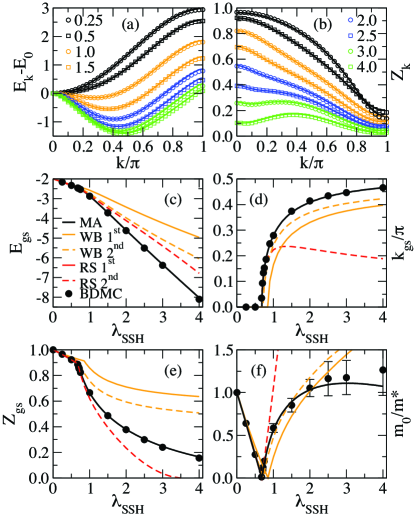
Figure 3: (color online) Results for the 1D SSH model with $\Lambda_{o}=0.75$. We show the same quantities as in Fig. 2; in (a) and (b) we show results for $\lambda_{SSH}$ ranging from 0.25 to 4.0.

We see that we are dealing here with a sharp transition between a weak- and a strong-coupling regime. The weak-coupling regime has a single non-degenerate ground state located at $k_{gs}=0$. Since the system is inversion symmetric, the strong-coupling regime is doubly degenerate, with ground state wave-vectors $\pm k_{gs}\neq 0$. As emphasized in Ref. PRL, , the transition arises from a non-analyticity in the function $E_{gs}(\lambda_{SSH})$ at $\lambda_{SSH}=\lambda^{*}_{SSH}$. The non-analyticity is clearly not associated with any localization or self-trapping of the polaron; nor is it a quantum phase transition. This is because although we work at $T=0$, we are only treating the single-electron case. A phase transition involves the cooperative behavior of a macroscopic number of degrees of freedom, which is simply impossible in the one-electron limit, where only a finite and rather small average number of phonons are associated with the single polaron cloud. It is of course possible that the transition we have found may evolve into a critical phase transition at a finite particle concentration; however we cannot support such claims based on the current data.

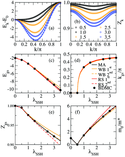
Figure 4: (color online) Results for the 1D SSH model, with $\Lambda_{o}=25$. We show the same quantities as in Fig. 2; in (a) and (b) we show results for $\lambda_{SSH}$ ranging from 0.5 to 3.5.

It remains to check how the results vary with the adiabaticity parameter $\Lambda_{o}$. In Figs. 3 and 4 we show all of the same results as those in Fig. 2, but now for $\Lambda_{o}=0.75$ and $25$. The main observations we can make here are:

(a) The basic behavior of the dispersion relation as a function of $\lambda_{SSH}$ is just as before, but as $\Lambda_{o}$ increases, the bandwidth steadily increases, and the effective mass $m^{*}(k_{gs})$ decreases - indeed, quite remarkably, for large $\Lambda_{o}$ the polaron is actually lighter than the bare band particle except in the region near the critical coupling, where its mass diverges. The transition is signaled as before by non-analytic behavior in all functions at $\lambda_{SSH}=\lambda^{*}_{SSH}$; the basic behavior of $k_{gs}$ and $E(k_{gs})$ as functions of $\lambda_{SSH}$ is similar to that for small $\Lambda_{o}$. Notice how well perturbation theory works in the extreme anti-adiabatic limit $\Lambda_{o}\gg 1$; the reason for this is discussed below.

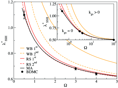
Figure 5: (color online) Transition line $\lambda^{*}_{SSH}$ vs. $\Omega_{o}$ in the pure SSH model, separating the weak-coupling regime, with its non-degenerate ground state at $k_{gs}=0$, from the strong-coupling regime with its doubly degenerate ground-state at $\pm k_{gs}\neq 0$. The inset shows the same data over a wider range of phonon energies. Results from BDMC, MA, and perturbational RS and WB of both $1^{st}$ and $2^{nd}$ order are shown. Other parameters are $\lambda_{H}=0,t_{o}=1$.

(b) As $\Lambda_{o}$ increases, the $qp$ weight is less and less affected by the non-diagonal coupling to the phonons, and is not much smaller than the free particle result $Z_{k}=1$; for $\Lambda_{o}\gg 1$, we see that $Z_{k}$ remains considerable even at very large couplings. This is of course the exact opposite of what happens in any diagonally coupled model, no matter what the form of $g(q)$.

(c) We also see that as $\Lambda_{o}$ increases, the transition coupling $\lambda^{*}_{SSH}$ slowly decreases. In Fig. 5, we show this behavior in more detail, by drawing the ”critical line” $\lambda^{*}_{SSH}(\Lambda_{o})$ as a function of the adiabaticity ratio, which separates the weak-coupling and strong-coupling regimes, and along which the effective mass diverges. All methods, even 1st-order perturbation theory, work well in the anti-adiabatic limit $\Lambda_{o}\gg 1$, where we see that $\lambda^{*}_{SSH}\rightarrow 0.5$, a result which we explain below.

On the other hand we do not show any numerical results for the adiabatic limit $\Lambda_{o}\rightarrow 0$ in Fig. 5, because all these methods become inaccurate here - note the large error bars for $\Lambda_{o}\ll 1$. This is because the average number of phonons in the polaron cloud increases rapidly with decreasing $\Lambda_{o}$, and the convergence of the BDMC code is then drastically slowed. MA results do converge, however the three-site cloud assumption becomes questionable in this limit. As noted in Ref. PRL, , LPBED results based on a five-site cloud restriction suggest that as $\Omega_{o}\rightarrow 0$, $\lambda^{*}_{SSH}$ actually reaches a maximum and then decreases. Thus what actually does happen for small $\Lambda_{o}$ is an open question. This region can be studied using other numerical methodsadia that have already been successfully applied to the Holstein model in the adiabatic limit.

(ii) Physics of the pure SSH polaron: The behavior discussed above is most easily understood if we begin from the anti-adiabatic limit, $\Lambda_{o}\rightarrow\infty$, where perturbation theory can be applied (for a preliminary discussion of this limit see Ref. PRL, ). Consider the first order contribution to the polaron self-energy, viz.:

$$\Sigma_{1}(k,\omega)={1\over N}\sum_{q}\frac{|V(k,q)|^{2}}{\omega+i\eta-\epsilon_{k-q}-\Omega_{o}}.$$

Since the range of $\epsilon_{k}$ is just the bandwidth, i.e., $\sim\mathcal{O}(t_{o})$, it follows that when $\Omega_{o}\gg t_{o},\omega$, the denominator is $\sim-\Omega_{o}$. The integral can then be carried out, and we find:

$$\lim_{\Lambda_{o}\rightarrow\infty}\Sigma_{1}(k,\omega)=-t_{o}\lambda_{SSH}[2-\cos(2k)]$$

Higher-order diagrams contributing to $\Sigma_{l}(k,\omega)$, i.e., containing $l$ internal phonon lines, scale as $(1/\Omega_{o})^{2l-1}$, and can thus be ignored for sufficiently large $\Lambda_{o}$ (note that we deal here with an asymptotic series - the number of diagrams at level $l$ is $\sim(2l-1)!!$, which for $l>\Lambda_{o}$ outweighs the factor $(1/\Omega_{o})^{2l-1}$; but for $\Lambda_{o}\gg 1$, this simply means that low-order perturbation theory gives very accurate results, divergentS unless we go to very long times). It then follows that the polaron energy $E_{k}=\epsilon_{k}+\Sigma(k,E_{k})$ in this limit is well approximated by:

$$E_{k}=-2t_{o}\lambda_{SSH}-2t_{o}\cos(k)+t_{o}\lambda_{SSH}\cos(2k).$$ (15)

In other words, apart from an overall shift, the energy contains both nearest-neighbor and second-nearest-neighbor hopping terms. The former favors a $k=0$ ground state, while the latter, because of its unusual sign, favors a ground state at $k=\pm{\pi\over 2}$, together with a “folded” dispersion. For small $\lambda_{SSH}$ the former term dominates, but if $\lambda_{SSH}$ is sufficiently large, the behavior is controlled by the phonon-mediated second-nearest-neighbor term. The transition takes place at the inflection point where the effective mass diverges, i.e., when:

$$\frac{m}{m^{*}(k=0)}=-2t_{o}[1-2\lambda_{SSH}]\;\rightarrow 0$$

explaining why, in Fig. 5, $\lim_{\Omega_{o}\rightarrow\infty}\lambda^{*}_{SSH}=0.5.$ These considerations are confirmed by the data shown in Fig. 4 for $\Omega_{o}=100t_{o}$. As expected, here all perturbative results agree well with the BDMC and MA results.

In physical terms, what has happened here is that the phonon-modulated hopping has opened a new “channel” for particle motion. Direct hopping of a particle away from its phonon cloud has an exponentially small probability when phonons are energetically costly. This is why in diagonal coupling models, with ${V}(k,q)=g(q)$, the effective hopping amplitude (and hence the inverse effective mass) is exponentially suppressed. However, in a non-diagonal hopping model with ${V}(k,q)=V(k,q)$, the particle can move phonons along as it hops. In the SSH model discussed here, the particle can hop to the neighboring site while creating a phonon on that site, and then hop one site further while absorbing this same phonon. This gives rise to an effective second nearest-neighbor hopping, i.e., we now have an effective low-energy band Hamiltonian for the polaron of form

$$E_{k}=t_{1}\cos k\;+\;t_{2}\cos 2k$$ (16)

where $t_{1}$ is the renormalized value of the bare $t_{o}$, and $t_{2}$ the effective 2^nd nearest-neighbor hopping term. The phonons have not gone away, of course, but for this lowest polaron band $\mbox{Im}\Sigma(k,\omega)=0$, since there are no lower states for the polaron to decay to. For the SSH model the transition at $\lambda_{SSH}=\lambda^{*}_{SSH}$ occurs because $t_{2}$ has a negative sign - the physical reason for this is that the phonon increases one bond length, but decreases the other (cf. discussion in Ref. PRL, ).

More complicated scenarios are found in other $g(k,q)$ models; however the underlying idea is the same. For example, in the Edwards model,Edwards ; PhysRevB.82.085116 ; Mono the particle first creates a string of three consecutive bosons and then goes back and removes them, again resulting in effective second nearest neighbor hopping (this time with a positive sign, so that there is no transition). Similar results are obtained in $t-J_{z}$ models.Holger2 Here, the particle goes twice around closed Trugman loops.Trloops On the first circuit it creates a string of bosons, which are all removed on the second circuit. This gives rise to both effective second- and third-nearest neighbor hopping.

Now consider what happens when $\Omega_{o}$ decreases. The one-phonon mechanism for the transition is then supplemented by processes involving more and more phonons, which will create not only second-nearest neighbor hoppings, but also longer-range hopping terms (and lead to increasing disagreement between low-order perturbation theory and the BDMC and MA results). Note that if the phonons modulate only the nearest neighbor hopping – as in the SSH model – then only terms $t_{2n}$ can be generated dynamically, because there must be an even number of hops to absorb all emitted phonons, and so the carrier cannot end up an odd number of sites away from its initial location without changing the number of bosons. The $t_{2n+1}$ terms are either renormalized bare terms, like $t_{1}$, or are generated by mixing with the continuum as $\Omega_{o}$ decreases and the band is flattened. Of course, in models where phonons modulate longer-range hopping and/or coupling is beyond linear, any $t_{n}$ can be generated dynamically.

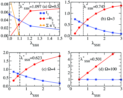
Figure 6: (color online) Effective hopping constants $t_{1}$ (squares) and $-4t_{2}$ (circles) in the SSH model, obtained from a fit of $E_{k}$ as described by Eq. (17), for (a) $\Omega_{o}=0.5t_{o}$, (b) $\Omega_{o}=3t_{o}$, (c) $\Omega_{o}=4t_{o}$ and (d) $\Omega_{o}=100t_{o}$. Triangles, shown only in (a), represents $\sum_{n=1}^{5}n^{2}t_{n}$. See text for more details.

To investigate this dynamical mechanism further we fit the polaron dispersion $E_{k}$, obtained from BDMC, to a functional form

$$E_{k}=-\sum_{n=0}^{5}2t_{n}\cos(nk),$$ (17)

up to fifth nearest-neighbor hopping. The results are shown in Fig. 6. For $\Omega_{o}=100t_{o}$, in panel (d), the fits agree with Eq. (15): $t_{1}\approx t_{o}$, $t_{2}\approx-t_{o}\lambda_{SSH}/2$, and the higher $t_{n\geq 3}$ are too small to show. As $\Lambda_{o}$ decreases, a fit to $E_{k}$ with only first and second nearest neighbor hopping remains acceptable, although the values of $t_{1}$ and $t_{2}$ deviate significantly from the asymptotic limits (compare panels (b) and (c)). The transition occurs when $t_{1}=-4t_{2}$; the crossing of these lines agrees well with $\lambda^{*}_{SSH}$ (dashed line), for these larger values of $\Lambda_{o}$.

However if we now go to $\Omega_{o}=0.5$, shown in panel (a), then longer-range hopping must be included to obtain reasonable fits. For simplicity, we continue to plot only $t_{1}$ and $-4t_{2}$. The $t_{1}$ and $-4t_{2}$ lines cross at a value above $\lambda^{*}_{SSH}$, because of the $n\geq 3$ hopping terms. The role of these terms can be seen directly if we compute the inverse effective mass $1/m^{*}(k=0)=\;\sum_{n=1}^{5}n^{2}t_{n}$. This value is shown by triangles, and it indeed vanishes at $\lambda^{*}_{SSH}$.

Clearly as $\Lambda_{o}$ decreases further it becomes impractical to try and unravel all the higher-order terms. This is why we cannot explain all the details of the transition in this limit, nor can we predict what happens as $\Lambda_{o}\rightarrow 0$ based on these methods and results.

Let us now summarize what we have found for the polaron with purely off-diagonal SSH coupling. Just as we saw that the physics of the diagonally-coupled polaron could be summarized in one key feature, viz., the smooth crossover from weak to strong coupling, with no intervening transition, we see that the non-diagonally coupled polaron’s behavior also turns on one key feature, viz., the range and sign of the phonon-mediated long-range hopping terms, which may lead to a sharp transition in polaron properties. The physics here is intrinsically more complicated because one can imagine a wide variety of scenarios, depending on the relative sizes and signs of the different terms. This will be particularly true in the quasi-adiabatic regime when $\Lambda_{o}$ is small, where we do not rule out a whole sequence of transitions as the bare off-diagonal coupling increases. In the simple SSH model studied here, there is only one transition in the regime we have studied, where we assume that $\Lambda_{o}$ is not too small - the reason for this was discussed above. But clearly these results constitute just the tip of the iceberg as far as possible different behaviors are concerned, and it will be interesting to study different off-diagonally coupled models, having different forms for $g(k,q)$.

V Dual-coupling model - combined Holstein and SSH couplings

In any real polaronic system there will generically be both diagonal and non-diagonal couplings between the electrons and the phonons (or whatever other kind of bosonic excitation is involved). Thus it is crucial to know how the competing (and very different) effects coming from each coupling end up working together. In what follows we investigate a combined ”Holstein + SSH” model, with both $\lambda_{H}$ and $\lambda_{SSH}$ finite. Note that even though Eqs. (8) and (10) suggest that the results depend on the sign of $g_{o}/\alpha_{o}$, this sign is in fact irrelevant. This is because, as we noted when discussing the sign problem, all contributions with odd powers in either $g_{o}$ and/or $\alpha_{o}$ cancel out. Thus the parameters $\lambda_{H}$ and $\lambda_{SSH}$ are sufficient to fully characterize the couplings in this model.

Before discussing our results, it is worthwhile trying to guess what might be the result of combining the couplings. If we take the ’effective band’ idea seriously, then one can argue that (i) the main effect of the diagonal coupling is to simply reduce the bandwidth of the ”$\cos k$” bare band, i.e., to severely renormalize the nearest-neighbor hopping $t_{o}$ down to $t_{1}$; and (ii) the main effect of the non-diagonal coupling is to create longer-range hopping terms of the form $t_{2n}\cos 2nk$. Thus everything will now depend on the relative strength of these terms - if we imagine first putting in the non-diagonal term, to create the long-range hoppings, and then add the diagonal term, we expect that not only will $t_{o}$ be renormalized down to $t_{1}$, but that there will also be a reduction of the higher $t_{n}$, for $n\geq 2$. Note that if the higher $t_{n}$ are renormalized down by the same factor as the renormalization of $t_{o}$ to $t_{1}$, the critical line $\lambda^{*}_{SSH}$ will be unchanged as a function of $\Lambda_{o}$: there will only be an overall weakening of all hopping amplitudes. However one can also imagine a scenario where the higher $t_{n}$ are less strongly reduced than $t_{o}$ - the critical coupling $\lambda^{*}_{SSH}$ will then be reduced from its value when there is no diagonal coupling. Conversely, if the $t_{n}$ are more strongly reduced, we expect $\lambda^{*}_{SSH}$ to increase. Which scenario will be exhibited is not a priori clear, nor is it clear how these results will depend on the adiabaticity ratio.

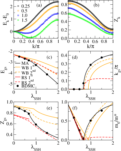
Figure 7: (color online) Polaron properties for the combined H/SSH model. We show the same plots as those shown in Fig. 2 for the pure SSH model, but now with a finite diagonal coupling $\lambda_{H}=0.25$. We choose $\Lambda_{o}=0.75,t_{o}=1$. In (a) and (b), the values of $\lambda_{SSH}$ are shown in the legend.

What is clear is that these questions are not going to be answered by perturbation theory. To find the transition line we return again to MA and BDMC results. In Fig. 7, we begin with data similar to that displayed earlier for the SSH model, i.e., plots of the variation of the quasiparticle behavior as a function of $k$ and of $\lambda_{SSH}$, but now for a small but finite $\lambda_{H}=0.25$. The results are shown here for the intermediate adiabatic ratio $\Lambda_{o}=0.75$. We see that the curves are not significantly changed from the pure SSH results by the addition of the diagonal coupling. This is further confirmed by the data shown in Fig. 8, for a larger diagonal coupling $\lambda_{H}=0.5$.

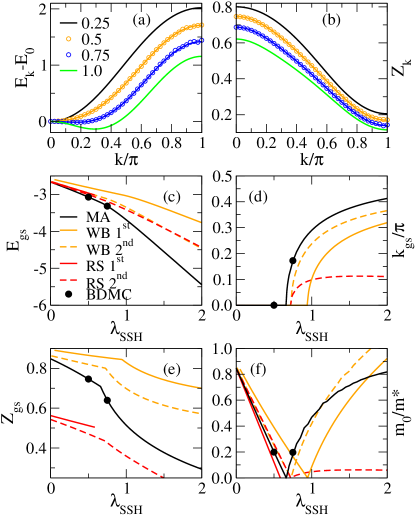
Figure 8: (color online) The same plots as in Fig. 7, but now for $\lambda_{H}=0.5$. As before, $\Lambda_{o}=0.75,t_{o}=1$. In (a) and (b), the values of $\lambda_{SSH}$ are shown in the legend.

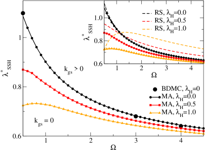
Figure 9: (color online) Transition coupling $\lambda^{*}_{SSH}$ vs. $\Omega_{o}$. MA results are shown for $\lambda_{H}=0$ (circles), $\lambda_{H}=0.5$ (squares) and $\lambda_{H}=1$ (triangles). Big circles show BDMC data for $\lambda_{H}=0$. The inset compares these values with those predicted by 2^nd order RS perturbation theory.

Above we discussed two possible scenarios for the behavior of the transition line as a function of the diagonal coupling. To see which of these is actually enacted, we show in Fig. 9, the transition value $\lambda^{*}_{SSH}$ as a function of $\lambda_{H}$. We see that the critical line moves down as we increase $\lambda_{H}$, i.e., the diagonal coupling suppresses the bare nearest-neighbor coupling more strongly than it does the higher nearest neighbor couplings.

Curiously, for larger $\lambda_{H}$ we see a peak in the critical line followed by a decrease in $\lambda^{*}_{SSH}$ at small $\Omega_{o}$; this is clear from the results for $\lambda_{H}=1$, and the $\lambda_{H}=0.5$ case is also consistent with the possible existence of a peak at even lower $\Omega_{o}$. This is reminiscent of the LPBED results found for $\lambda_{H}=0$ at $\Lambda_{o}<0.125$ (see Fig. 4 of Ref. PRL, ). As before, we emphasize that our results are not accurate in the limit of small $\Lambda_{o}$; however it is interesting that they suggest that such a peak followed by a decrease as $\Omega_{o}\rightarrow 0$ may actually be the typical behavior of $\lambda^{*}_{SSH}$ in the adiabatic limit.

We also show, in the inset of Fig. 9, how the 2^nd-order RS perturbation theory compares against the MA predictions. There is no reason to expect perturbation theory to be accurate away from the anti-adiabatic limit, and indeed that is the case for $\lambda_{H}\neq 0$; we believe that the excellent agreement for $\lambda_{H}=0$ is accidental.

These results give only a partial characterization of the transition behavior. For a full characterization, we need a map of the critical surface $\mbox{\boldmath$\lambda$}^{*}(\Lambda_{o})$, where $\mbox{\boldmath$\lambda$}^{*}\equiv(\lambda_{SSH}^{*},\lambda_{H}^{*})$ is the locus of values of the 2-dimensional coupling $\mbox{\boldmath$\lambda$}=(\lambda_{SSH},\lambda_{H})$ upon which the effective mass diverges. Clearly a complete map of this critical surface is a large undertaking, but just as one can produce a set of curves of $\lambda^{*}_{SSH}(\Lambda_{o})$ for different fixed values of $\lambda_{H}$, one can also do the converse, i.e., produce a set of curves of $\lambda^{*}_{H}(\Lambda_{o})$ for different fixed values of $\lambda_{SSH}$.

This is what Fig. 10 does, showing two such curves for $\lambda_{SSH}=0.7$ and $0.8$. Since the minimum value of $\lambda^{*}_{SSH}(\Lambda_{o})$ is $0.5$, as we reduce $\lambda_{SSH}$ the region occupied by the polaron dispersion with a $k_{gs}=0$ minimum should grow, and when $\lambda_{SSH}\leq 0.5$ it should fill the entire parameter space. Fig. 10 confirms this expectation, and we see that here a solution for a fixed $\lambda_{SSH}$ exists only if $\Lambda_{o}$ is sufficiently small. This is unlike Fig. 9, where a solution exists for a given $\lambda_{H}$ at any $\Lambda_{o}$ (excluding, possibly, the strongly adiabatic region).

For $\lambda^{*}_{H}=0$ and $\lambda_{SSH}=0.8$ the transition is at $\Omega_{o}\approx 1.53$, in agreement with Fig. 9. As $\lambda^{*}_{H}$ is increased, the transition line moves towards lower $\Omega_{o}$, enclosing the region where the ground-state has the minimum at $k_{gs}=0$. As $\lambda_{SSH}$ decreases, this region indeed grows and should asymptotically fill the entire phase-space.

This completes our detailed discussion of numerical and perturbative results for the dual-coupling H/SSH model.

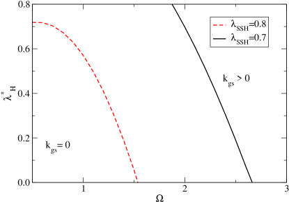
Figure 10: (color online) Transition coupling $\lambda^{*}_{H}$ vs. $\Omega_{o}$ for the H/SSH model. MA results are shown for $\lambda_{SSH}=0.7$ (full line) and $\lambda_{SSH}=0.8$ (dashed line).

VI An ’Effective Band’ paradigm for polarons

It is convenient to summarize all of these results in a new effective theory for the polaron in its lowest band. We will see that this picture is actually rather simple in the regime where $\Lambda_{o}=\Omega_{o}/4t_{o}>1$, i.e., where the phonons do not overlap with the bare band.

VI.1 Key features of the Dual Coupling Model

Let us first consider the main features of our dual coupling model results. We single out here the following as being most revealing:

(i) Ground-state momentum: In a purely diagonal coupling model, nothing happens to the ground-state momentum - we always have $k_{gs}=0$. In the non-diagonal SSH model, $k_{gs}$ departs rapidly from zero when we exceed the critical coupling $\lambda^{*}_{SSH}$ (itself a function of $\Lambda_{o}$). In the dual coupling model, a non-zero $k_{gs}$ is found everywhere above the critical surface $\mbox{\boldmath$\lambda$}^{*}(\Lambda_{o}$).

(ii) Ground-state effective mass: In a purely diagonal model like Holstein, the effective mass at the bottom of the lowest band varies smoothly for any coupling strength - there is no ’band collapse’, only a rapidly decreasing bandwidth and rapidly increasing effective mass, for large $\lambda_{H}$. In the purely non-diagonal SSH model, however, the mass does not become very large for large coupling $\lambda_{SSH}$. Instead it continues to be of roughly the same magnitude as the bare mass, except near the critical line $\lambda^{*}_{SSH}(\Lambda_{o})$, where it increases sharply, diverging to infinity right on this line. For the dual coupling model, viewed as a combined function of the dual coupling $\mbox{\boldmath$\lambda$}(\Lambda_{o})$, we see these two behaviors combined - the effective mass increases as before with $\lambda_{H}$, and for a given fixed value of $\lambda_{H}$, it varies only slowly with changing $\lambda_{SSH}$, except near the critical surface $\mbox{\boldmath$\lambda$}^{*}(\Lambda_{o})$ where $m^{*}(k_{gs})$ diverges.

We emphasize yet again that no phase transition is involved here - all that is happening is a change in the band shape, so that at a critical value of the coupling, the band mass at one specific value of momentum diverges.

(iii) Critical surface: The position of the critical surface depends only weakly on the adiabaticity parameter $\Lambda_{o}$ for sections with constant $\lambda_{H}$, although varying $\lambda_{SSH}$ can change things rapidly, as shown in Fig. 10. Further work needs to be done to clarify this in the adiabatic limit. We see that it is useful to think of the physics of the dual-coupled model in terms of this critical surface. However, this leaves unanswered the more fundamental question of what controls the surface.

(iv) Shape of Lowest Band: This question is answered if we look at the bandshape. For diagonal coupling only, the shape of the lowest polaron band will not be strongly affected by the coupling to the phonons if $\Lambda_{o}=\Omega_{o}/4t_{o}>1$ (in one dimension). The band will narrow as we increase the coupling, and the $\cos k$ form will be weakly distorted by higher-order phonon terms, but $m^{*}(k=0)$ will simply decrease smoothly as we increase the effective coupling, and the bottom of the band will remain at $k=0$.

When we have non-diagonal couplings, large longer-range hoppings are generated, which radically alter the band shape. This happens even when $\Lambda_{o}\gg 1$ (cf. Fig. 4). Moreover, the overall bandwidth does not become arbitrarily small with increasing effective coupling, like for diagonal coupling, but remains considerable.

In the dual coupling model, we see that these two mechanisms work relatively independently: the diagonal couplings cause a rapid but smooth contraction of the bandwidth, with little change in the bandshape, whereas the non-diagonal couplings alter the bandshape and prevent the bandwidth from narrowing excessively.

VI.2 The effective band Hamiltonian

Perhaps the most important insight to come from the studies recounted here is that, provided the phonon excitations do not overlap the lowest band (i.e., assuming $\Lambda_{o}>1$), we can understand all of the numerical results for the lowest polaron band in terms of a polaron band energy $E_{k}$ characterized by a set of effective hopping parameters $t_{n}(\mbox{\boldmath$\lambda$},\Lambda_{o})$ (compare discussion in section IV.B, and Eq. (17)).

VI.2.1 Quasiparticle picture

This suggests the following more general ansatz for the polaron problem with both diagonal and non-diagonal couplings, when $\Lambda_{o}>1$. Suppose we start from a dual-coupling model having the general form in Eq. (5), in which the phonons are assumed to be optical in nature, i.e., with a gap energy $\Omega_{o}$. However, we make no special assumptions about the form of $V(k,q)$, so that now we have a starting Hamiltonian

$$\hat{\mathcal{H}} = -\sum_{k}\epsilon_{k}~{}c_{k}^{\dagger}c_{k}+\sum_{q}\Omega_{o}b_{q}^{\dagger}b_{q}$$ (18)

$$+ \frac{1}{\sqrt{N}}\sum_{k,q}V(k,q)\;c_{k-q}^{\dagger}c_{k}\big{(}b_{q}^{\dagger}+b_{-q}\big{)},$$

where $\epsilon_{k}$ is the bare band dispersion (before coupling to phonons).

Then we argue that for analysis of the low-energy polaron physics, we can replace the Hamiltonian ${\cal H}$ in (18) by an effective Hamiltonian ${\cal H}_{\rm eff}$ having the general form

$$\hat{\mathcal{H}}_{\rm eff} = \sum_{k}\tilde{\varepsilon}_{k}\tilde{C}_{k}^{\dagger}\tilde{C}_{k}+\sum_{q}\tilde{\Omega}_{o}\tilde{B}_{q}^{\dagger}\tilde{B}_{q}$$ (19)

$$+ \frac{1}{\sqrt{N}}\sum_{k,q}\tilde{W}(k,q)\;\tilde{C}_{k-q}^{\dagger}\tilde{C}_{k}\big{(}\tilde{B}_{q}^{\dagger}+\tilde{B}_{-q}\big{)},$$

where ’tildes’ denote renormalized quantities. As we saw previously, if we start with a simple nearest-neighbor hopping in one dimension (so $\epsilon_{k}=-2t_{o}\cos k$), the renormalized band energy takes the form

$$\tilde{\varepsilon}_{k}^{(1d)}\;=\;-2\sum_{n}\tilde{t}_{n}(\mbox{\boldmath$\lambda$},\Lambda_{o})\cos kn$$ (20)

in which $\tilde{t}_{1}$ is the renormalized value of $t_{o}$, and the $\tilde{t}_{n}$ are the set of new multi-site hopping parameters which have been created by the non-diagonal coupling to phonons; the operators $\tilde{C}_{k}$ create these new effective band ’quasiparticles’. The other terms in Eq. (19) describe a set of ’continuum’ excitations, created by the bosonic operators $\tilde{B}_{q}$, with renormalized energy $\tilde{\Omega}_{o}$, and a renormalized ’hybridization’ coupling $\tilde{W}(k,q)$ between the band quasiparticles and the continuum excitations. There are new energy scales in this effective Hamiltonian - a renormalized interaction $\tilde{W}(k,q)$ between the effective band, with renormalized bandwidth $\tilde{D}\sim\mathcal{O}(\tilde{t}_{1})$, renormalized gap $\tilde{\Omega}_{o}$ to continuum excitations, and a renormalized adiabaticity parameter $\tilde{\Lambda}_{o}=\tilde{\Omega}_{o}/\tilde{D}$.

The key advantage of this quasiparticle picture is that except in the effective anti-adiabatic regime, where the effective adiabaticity parameter $\tilde{\Lambda}_{o}<1$, the renormalized coupling $\tilde{W}(k,q)$ plays little role - it is considerably smaller than the original $V(k,q)$, most of whose effects have already been absorbed into the renormalized band. What this means is that unless $\tilde{\Lambda}_{o}\sim\mathcal{O}(1)$ or less, the effective band energy $\tilde{\varepsilon}_{k}$ will differ very little from the exact $E_{k}$ that one finds in either an exact numerical calculation, or in experiments. Thus we will find that

$$\tilde{t}_{n}\sim t_{n}\;\;\;\;\;\;\;\;(\tilde{\Lambda}_{o}>1)$$ (21)

where the coefficients $\{t_{n}\}$ are extracted from fitting to the exact band dispersion $E_{k}$ (or numerical approximations to it). Only when, as $\tilde{\Lambda}_{o}$ is decreased, the continuum states approach the top of the effective band, will there be significant differences between $\tilde{\varepsilon}_{k}$ and $E_{k}$, because of level repulsion between the effective band and the continuum excitations. The quasiparticle picture discussed here assumes that $\tilde{\Lambda_{o}}>1$ is always satisfied.

We make no attempt here to determine the parameters in this effective Hamiltonian as functions of the underlying parameters in Eq. (5). The philosophy we adopt is similar to that involved in, eg., the Landau Fermi liquid theory: the parameters in $\hat{\mathcal{H}}_{\rm eff}$ are ultimately to be determined by experiment on specific system(s), where possible; one predicts the results for different experiments in terms of the $\tilde{t}_{n}$, and uses the results to determine the $\tilde{t}_{n}$.

Thus the form given above for $\hat{\mathcal{H}}_{\rm eff}$ constitutes a hypothesis for the results of both experiments and non-perturbative numerical work, and is thus in principle testable. The key result in the present work, as we saw in section IV.B, is that all of the features found here in the dual coupling model can be understood in terms of the behavior of the $\{t_{n}\}$ defined in (17); the following aspects are particularly important:

(a) If we only have diagonal couplings in the model, then only $\tilde{t}_{1}$ exists in the sum of Eq. (20) and we have a very simple band polaron, whose bandwidth and effective mass vary continuously with coupling strength. The actual dispersion $E_{k}$ will hardly differ from the quasiparticle form $\tilde{\varepsilon}_{k}=-2\tilde{t}_{1}\cos k$ (in one dimension) when $\tilde{\Lambda}_{o}$ is large; only when the continuum gap energy $\tilde{\Omega}_{o}\sim\tilde{t}_{1}$ will we see a distortion of the simple cosine form for the band dispersion. To see this, consider Fig. 1 (c), where $\lambda_{H}=1$ in the Holstein model; the distortion of $E_{k}$ away from a simple cosine form, caused by the continuum states, is quite small even when $\Lambda_{o}$ is as small as $0.5$. This is because here $\tilde{t}_{1}<0.15t_{o}$, so that the renormalized adiabaticity parameter $\tilde{\Lambda}_{o}\sim 1$; the continuum is well above the lower quasiparticle band. For large diagonal coupling, the $\cos k$ form for the quasiparticle band will be accurate except for very small $\Omega_{o}$.

(b) Introducing a non-diagonal coupling generates the $\tilde{t}_{n}$ with $n=2,3,...$; with increased coupling strength, they become steadily more important. If their signs are negative, a transition to a new polaron with finite $k_{gs}$ is eventually achieved, once $|\tilde{t}_{2}|$ outweighs $\tilde{t}_{1}$; as $|\tilde{t}_{2}|/\tilde{t}_{1}$ increases further, $k_{gs}\rightarrow\pi/2$. A key result comes out of the H/SSH model, where we saw that increasing the diagonal coupling $\lambda_{H}$, while keeping the non-diagonal coupling $\lambda_{SSH}$ constant, suppresses the lowest-order hopping term $t_{1}$ faster than it does the higher terms $t_{2},t_{3}$, etc. This then makes it easier for the system to make the transition (i.e., it then happens for a smaller value of $\lambda_{SSH}$). The renormalized band, now parametrized in terms of the $\{\tilde{t}_{n}\}$ simply evolves in shape as $\lambda_{SSH}$ increases. For any finite diagonal $\lambda_{H}$, the bandwidth remains finite, no matter what is the non-diagonal $\lambda_{SSH}$.

(c) The transition line in no way marks any kind of quantum critical point, or collapse of the bandwidth. It simply marks the locus of points where the ground state momentum starts to shift away from zero. The renormalized bandwidth is never zero (see the plots of $E_{k}$ in Figs. 2-4, 7, and 8); although the $k=0$ effective mass diverges along the transition line, this is simply because $k=0$ then marks a point of inflection of the dispersion relation $E_{k}$, at which $\partial^{2}E_{k}/\partial k^{2}=0$. The renormalized adiabaticity ratio $\tilde{\Lambda}_{o}$ also is finite at the transition point.

VI.2.2 Transitions in the band structure

We have already remarked above that the transition found here is completely unconnected with the rapid crossover found in the polaronic bandwidth as $\lambda_{H}$ is increased - indeed there is never a transition as a function of $\lambda_{H}$. It also seems unlikely that anything in particular should happen to the electron-phonon entanglement at the transition we have found, since the effective band structure is varying continuously, and certainly for $\Lambda_{o}\gg 1$, nothing special happens to the mixing between the polaronic band and the higher energy continuum. In this connection we note that Ref. stojan08, finds some sort of transition in the entanglement between the polaron and the phonons, however we believe that what they have found is unconnected to the transition discussed here. This is because unlike what we find, their transition only occurs for sufficiently small $\Lambda_{o}$, and even when present it is at different values of the coupling.

We emphasize that one expects to see rather complicated effects when the lowest polaron quasiparticle band begins to overlap with the optical phonon - at this point level-crossing and real transitions become possible, with a large scale reorganization of states at the top of the polaron band. This is not a quantum phase transition, at least in the conventional sense of the term (indeed, if one applied the term to describe this overlap of states for a single quasiparticle, it could also be applied to describe a wide variety of chemical and nuclear reactions, which would completely divest it of its original significance).

VII Conclusions: More General Models, and Experiments

All the concrete results found in sections IV and V were for the dual H/SSH model. However this model is still fairly specialized; it involves only couplings linear in the phonon variables, and couples electrons to gapped optical phonons only. How general are such results, and what might they have to do with experiments on real systems? Let us look at these questions in turn.

VII.1 More general couplings

We can obviously ask what happens if (i) we go to more general models with combined diagonal and non-diagonal couplings, and (ii) if we also include acoustic phonons, and even perhaps higher-order phonon terms, such as the quadratic couplings in Eq. (2).

Once we look at the system in terms of the effective band Hamiltonian, it becomes clear that there is almost certainly a lot more interesting physics to be revealed in dual coupling models of this kind. This is because there is no reason in principle why one cannot imagine a destabilization of the $k_{gs}=0$ groundstate to other ground states in which, for example, the $t_{3}$ hopping term dominates (which could, as $t_{3}$ began to dominate over $t_{1}$, have a $k_{gs}\rightarrow\pi/3$ or $2\pi/3$). In this way one can envisage a hierarchy of states, each having a different groundstate momentum, with critical lines/surfaces existing between them. Clearly, to see this full complexity, one would have to begin by allowing modifications of the form of the diagonal and non-diagonal couplings $g_{1}({q}),g_{2}({k},{q})$, thereby exploiting the full freedom allowed by the momentum dependence of each - the Holstein and SSH coupling forms are merely the simplest that one can imagine. One way to get more interesting physics of this kind would be looking for non-diagonal couplings $g_{2}({k},{q})$ with longer-range in real space, i.e., with a more sharply-peaked behavior in momentum space. Thus a fairly clear prediction arising from our effective Hamiltonian is that of possible multiple ”effective band” transitions as one varies the non-diagonal couplings.

Another possibility, recently demonstrated in a model combining SSH and BM coupling,MAca appears when the diagonal coupling is also longer-range. In such cases, interference between the two couplings can lead to additional renormalization of $t_{o}$ and even change its sign. For example, in the limit $\Lambda_{o}\gg 1$ of Ref. MAca, , this occurs through processes where SSH coupling moves the electron to a neighboring site while emitting a phonon at the original site, and then BM coupling absorbs that phonon without changing the electron location (the order of the two processes can be reversed and the contributions add up). This generates an additional contribution to $t_{1}$ whose sign is controlled by the product of the two couplings. If it is negative and if its magnitude is large enough, one expects to see a second transition to a $k_{gs}=\pi$. Indeed, this was observed in Ref. MAca, .

The way in which any coupling to acoustic phonons and phonon pair excitations might affect these results is an interesting question. We tend to believe that they will only further renormalize the effective band energy $\tilde{\varepsilon}_{k}$, as well as introduce dissipative processes for arbitrarily low energy, but that they will not alter the basic result that non-diagonal coupling to optical phonons can reorganize the band and change the ground-state momentum. However, this question merits further study.

Finally, it is now known that even small non-linear coupling to phonons, of the Holstein type (i.e. local in real space) has significant effects both on the physics of the single polaron,clemens and at finite carrier concentrations.steve It should be clear from the above discussion that such non-linear terms in either kind of coupling may open additional channels to generate longer-range hoppings. Whether this can lead to qualitatively different behavior from that discussed above for linear couplings is another question that merits further study.

VII.2 Experiments and Conclusions

So far, we have not discussed the experimental relevance of our work. The main reason is that, apart from a few notable exceptions,troisi07 both computational efforts to calculate these couplings and the models used to extract such couplings from fits of experimental measurements tend to focus on a pure model, i.e. either on only diagonal or only non-diagonal coupling. What would be far preferable would be attempts to compare theory and experiment directly, using the kind of computations discussed here - experiments would allow one to extract the renormalized parameters rather than the bare ones, and they will be quite different if the couplings are strong. It almost goes without saying, in view of the results found here, that any attempt to compare experiments with theories which do not include the effect of Peierls couplings is likely to give very misleading results.

A different avenue is opened by the use of cold atoms and/or polar molecules trapped in optical lattices as simulators of such mixed Hamiltonians.Herrera ; MAca ; RK1 ; RK2 As typical in such systems, they would permit the tuning of individual coupling strengths within wide ranges, such that properties like those discussed here could be investigated in a significant area of the parameter space.

To conclude, we have given a fairly exhaustive characterization of the behavior of polarons in the dual coupling H/SSH model, in terms of an ’effective band’ paradigm, in which diagonal interactions cause a continuous narrowing of a low-energy quasiparticle band, and non-diagonal interactions add non-local hopping terms to this band, which gradually change its shape, and eventually force the ground state to move, at a definite transition point, to non-zero momentum. Indeed, we see no evidence for, nor any theoretical reason to expect, any sudden changes to the polaronic band, for any value of either diagonal or non-diagonal coupling to phonons. The effective band quasiparticle picture works if the phonon energy is larger than the renormalized bandwidth - otherwise level mixing between the phonons and the polaronic states gives a more complicated picture. The behavior of physical quantities in an H/SSH model will typically be rather different from what one expects from a simple Holstein model, and this needs to be taken into account in comparison between theory and experiment.

Appendix A Bold Diagrammatic Monte Carlo technique

We herein distinguish between methods sampling the Green’s function ($G$-DMC), and the self-energy ($\Sigma$-DMC). The Bold Diagrammatic Monte Carlo (BDMC) algorithm is essentially a $\Sigma$-DMC method, but relies on a faster sampling based on a self-consistent procedure relying on Dyson’s identity PhysRevLett.99.250201 ; PhysRevB.77.020408 ; PhysRevB.77.125101 . In this appendix, we provide a more detailed summary of our own implementation to polaron problems.

A.1 Green function, self-energy and diagrammatics

The main quantity of interest here is the $T=0$ retarded polaron Green function. We write this as

$$G(t,\,k,\,\mu)=-i\Theta(t)\sum_{n}e^{-it\big{(}E_{n}(k)-\mu\big{)}}|\langle n,\,k|k\rangle|^{2},$$ (22)

in terms of eigenstates $|n,\,k\rangle$ and $E_{n}(k)$ of the full Hamiltonian; here $\mu$ is the chemical potential, which for this one-electron system is just an overall shift in energy. In the absence of interactions this reduces to $G_{0}(t,\,k,\,\mu)=-i\Theta(t)e^{-it\big{(}\epsilon(k)-\mu\big{)}}$. In the frequency domain we write

$$G(\omega,\,k,\,\mu)=\sum_{n}\frac{Z_{n}(k)}{\omega-E_{n}(k)+\mu+i\eta},$$ (23)

with infinitesimal $\eta>0$.

As noted by Prokof’ev et al., the sign problem can be avoided by analytic continuation of the Green’s function to imaginary time $\tau=it$, and corresponding imaginary frequency $\xi=-i\omega$, so that the exponential in (22) is real and positive definite. However, the analytic continuation and the Fourier transformation do not commute. Writing PhysRevB.77.020408 $G^{i}(\xi,\,k,\,\mu)=G(\omega=i\xi,\,k,\,\mu)$, we define the imaginary time Green’s function to be

$$G^{i}(\tau,\,k,\,\mu)=-iG(t=-i\tau,\,k,\,\mu),$$ (24)

where the superscript $i$ denotes imaginary quantities. For convenience we actually calculate $\tilde{G}^{i}(\tau,\,k,\,\mu)=-G^{i}(\tau,\,k,\,\mu)$. Fig. 11 shows $G^{i}(k,\,\tau)$ up to second order diagrams. The relevant indices which need to be sampled are shown only for the first order diagram.

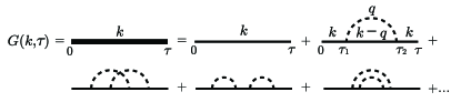
Figure 11: Diagrams contributing to $G^{i,\,1^{\textrm{\tiny st}}}(\tau,\,k)$. Relevant indices are only shown for the the first few diagrams. Each phonon propagator $i$ has a momentum $q_{i}$, and each electron propagator $j$ has a momentum $k_{j}=k-\sum_{i^{\prime}\in\{j\}_{i^{\prime}}}q_{i^{\prime}}$ where $\{j\}_{i^{\prime}}$ is the set of phonons propagators covering the electron propagator $i^{\prime}$

For $\Sigma$-DMC and BDMC we need to use the proper self-energy, defined as usual by organizing $G^{i}$ diagrams as blocks of inseparable phonon tangles linked by bare electron propagators, so that the self-energy is the sum of all possible diagrams that cannot be separated into a number of pieces by cutting only an electron line. Then Dyson’s equation in imaginary frequency reads

$$G^{i}(\xi,\,k,\,\mu)=\frac{1}{G^{i\>\>-1}_{0}(\xi,\,k,\,\mu)-\Sigma^{i}(\xi,\,k,\,\mu)},$$ (25)

where $\Sigma^{i}(\xi,\,k,\,\mu)$ is the Fourier transform of $\Sigma^{i}(\tau,\,k,\,\mu)$. Prokof’ev and Svistunov showed PhysRevB.77.125101 that most of the relevant observables can be extracted directly from the imaginary time self-energy without using Dyson’s equation first to obtain the Green’s function; $\Sigma^{i}(\xi,\,k,\,\mu)$ is calculated with the DMC algorithm using similar diagrammatic rules to those of $G$-DMC for propagators and the interaction vertices, but now using the topology of the $\Sigma$ diagrams. Each diagram included in $\Sigma$ corresponds to an infinite number of diagrams in $G$, making $\Sigma$-DMC much more efficient.

A.2 MC Sampling, normalization and orthonormal functions

In both $G$-DMC and $\Sigma$-DMC. it is useful to introduce a constant shift in energy $\mu$ to allow for a good sampling of diagrams with larger imaginary time. In both $G$-DMC and $\Sigma$-DMC. In $G$-DMC, normalization is most easily achieved using $\tilde{G}^{i}(\tau=0,\,k)=1$. We similarly can normalize $\tilde{\Sigma}^{i}(\tau,\,k,\,\mu)=-\Sigma^{i}(\tau,\,k,\,\mu)$ using

$$\tilde{\Sigma}^{i}(\tau=0,\,k)=\frac{1}{2\pi}\int_{0}^{2\pi}\!\!\textrm{d}q\,g(k-q,\,q)g(k,\,-q),$$ (26)

which differs from $\tilde{G}^{i}(\tau=0,\,k)$ due to the contribution of two vertices. This is the approach used in this work. Alternative normalization schemes consist in enlarging the configuration space with unphysical diagrams that can be calculated analytically or selecting a subset of the physical diagrams that can be calculated analytically. The other diagrams are then normalized by calculating the ratio between this normalization sector and the rest of the configuration space.

The accuracy of the normalization and of the data collected will depend closely on the histogram spacing used. A notable improvement over a simple histogram is to use a bin size increasing with $\tau$, giving a better sampling at small times for an accurate normalization, while accumulating enough points per bin at large $\tau$ to average over statistical noise. When collecting statistics with variable-size bins, we need to include a factor of $1/\delta\tau$, with $\delta\tau$ the size of the bin.

A further improvement consists in expanding the function sampled over the range of each bin with a set of orthonormal functions $F_{n}(\tau-\tau_{m})$ centred at the bin centre $\tau_{m}$. An arbitrary function $f(\tau)$ can be written as

$$f(\tau)=\sum_{a}c_{a}F_{a}(\tau-\tau_{m})+\textrm{correction},$$ (27)

for $\tau\in[\tau_{m}-\delta\tau/2,\,\tau_{m}+\delta\tau/2]$, with coefficients $c_{a}$. A finite set of functions is sufficient if the bin size $\delta\tau$ is not too large, and if the function is smooth on this range. The Gram-Schmidt orthogonalization procedure can be used to normalize the chosen set. The functions used herein are the Legendre polynomials $P_{n}(\tau-\tau_{m})$, but normalized such that $\int_{-\delta\tau/2}^{\delta\tau/2}\textrm{d}\tau F_{a}^{2}(\tau)=1$, instead of the usual $P_{n}(1)=1$. Collecting statistics for a specific bin is now done for each coefficient $c_{a}$. After an update, if the diagram has a length that falls on the bin’s range, each coefficient is updated with

$$c_{a}\to c_{a}+F_{a}(\tau-\tau_{m}).$$ (28)

A.3 Updates

The minimal set of updates is similar to $G$-DMC. The set must include updates to insert and delete phonons, and an update to change the total length of the self-energy diagram. We must start with at least one phonon and we cannot allow this first phonon to be removed; so an extra update to change the momentum of this first phonon is needed. The absence of the bare propagator before and after the proper self-energy part means that the insertion of a phonon must now allow for a change of the diagram length by considering also phonons inserted past the current length of the diagram. Each type of update is assumed to be chosen with equal probability $1/4$. We refer below to the current diagram with all its specific values for time and momentum indices as $\nu$, and to the suggested updated diagram as $\nu^{\prime}$, while $W_{\nu}$ ($W_{\nu^{\prime}}$) are the weights of the current (updated) diagram.

Phonon insertion and deletion can be balanced together. For insertion, we sample the momentum uniformly over $[0,\,2\pi[$, then choose the time of the first vertex $\tau_{1}$ uniformly on $]0,\,\tau]$ with $\tau$ the time of the final vertex of the diagram $\nu$ . We use the value of the phonon propagator $\propto e^{-\omega(q)(\tau_{2}-\tau_{1})}$ to sample the time of the second vertex between $[\tau_{1},\,\tau_{\textrm{\tiny max}}]$, where $\tau_{\textrm{\tiny max}}$ is some fixed cutoff. This keeps the probability distribution closer to the ratio of weights, but ignores the more complicated values of the electron propagators. The exponential distribution also prevents too many update suggestions that would result in very long and costly diagrams. The resulting probability distribution for inserting a specific phonon is then

$$\mathcal{P}_{\textrm{\small insert}}=\frac{1}{4}\cdot\frac{1}{2\pi}\cdot\frac{1}{\tau}\cdot\frac{\omega(q)e^{-\omega(q)(\tau_{2}-\tau_{1})}}{1-e^{-\omega(q)(\tau_{\textrm{\tiny max}}-\tau_{1})}}.$$ (29)

The inverse update, deletion, simply selects one phonon out of the $n_{\textrm{\tiny ph}}$ phonons not including the first one, with a probability of

$$\mathcal{P}_{\textrm{\small delete}}=\frac{1}{4}\cdot\frac{1}{n_{\textrm{\tiny ph}}-1}.$$ (30)

The acceptance ratios for the updates are therefore

$$R_{\textrm{\small insert}}=\mathcal{F}(\nu^{\prime})\cdot\frac{W_{\nu^{\prime}}}{W_{\nu}}\frac{2\pi\tau}{n_{\textrm{\tiny ph}}}\cdot\frac{1-e^{-\omega(q)(\tau_{\textrm{\tiny max}}-\tau_{1})}}{\omega(q)e^{-\omega(q)(\tau_{2}-\tau_{1})}},$$ (31)

$$R_{\textrm{\small delete}}=\mathcal{F}(\nu^{\prime})\cdot\frac{W_{\nu^{\prime}}}{W_{\nu}}\frac{(n_{\textrm{\tiny ph}}-1)}{2\pi\tau}\cdot\frac{\omega(q)e^{-\omega(q)(\tau_{2}-\tau_{1})}}{1-e^{-\omega(q)(\tau_{\textrm{\tiny max}}-\tau_{1})}},$$ (32)

where the extra factor

$$\mathcal{F}(\nu^{\prime}) = \>1\quad\textrm{if $\nu^{\prime}$ is a proper $\Sigma$ diagram}$$ (33)

$$\>0\quad\textrm{otherwise},$$

prevents improper diagrams from being generated.

In our own implementation we actually replace the update to change the length of the diagram by a more general update that will shift any vertex to a new time. We first select one of the vertices at random, except for the first one which we will keep fixed at $\tau=0$, and then select a new position for this vertex anywhere between the previous vertex and the next one. The last vertex is a special case for which we will select a new position between the previous one and a maximum $\tau_{\textrm{\tiny max}}$. In its simplest version, the position is uniformly distributed such that the acceptance ratio is simply the ratio of the weights.

Finally the update to change the momentum of a phonon simply selects one of the phonons and changes the momentum from its previous value to any other value with equal probability, again with an acceptance ratio equal to the ratio of the weights.

Given that we never remove the first phonon, ergodicity for the special case of a Hamiltonian with more than one branch will require an extra update to change the phonon branch of a specific phonon.

A.4 BDMC, bold line and double-counting

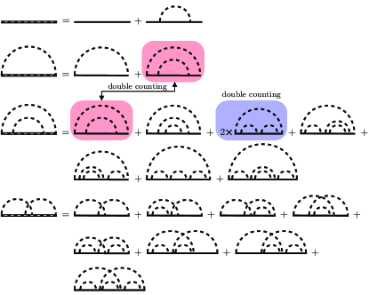
Figure 12: Drawing first and second order self-energy diagrams with a more complicated (bold) propagator composed of the bare propagator and first order Green’s function diagrams. The bold propagator is shown as a dashed thick line. The diagrams are assumed to be in frequency space such that the length of a propagator does not matter.

Fig. 12 shows how we implement the BDMC algorithm. The first-order diagrams for the self-energy generated with the thick ”bold” line give two diagrams while the two second-order diagrams now account for 15 types of diagrams. We have, however, double-counted 2 types of diagrams up to this order, something that needs to be forbidden to obtain the correct answer. To improve the bold propagator self-consistently the BDMC algorithm goes as follows:

• Initialize $\tilde{G}^{i}_{\approx}(\tau,\,k,\,\mu)=\tilde{G}^{i}_{0}(\tau,\,k,\,\mu)$ for a set $\{k\}$.

• Draw a first diagram for each $k$.

• MC sampling of diagrams for $\tilde{\Sigma}^{i}(\tau,\,k,\,\mu)$ for each $k$. Diagrams are drawn using $\tilde{G}^{i}_{\approx}$. Repeat $n$ times.

• Fourier transform $\tilde{\Sigma}^{i}(\tau,\,k,\,\mu)$ to get $\tilde{\Sigma}^{i}(\xi,\,k,\,\mu)$.

• Use Dyson equation to get $\tilde{G}^{i}_{\approx}(\xi,\,k,\,\mu)$.

• Fourier transform back to get a new $\tilde{G}^{i}_{\approx}(\tau,\,k,\,\mu)$.

• Go back to step 3 until convergence $\tilde{G}^{i}_{\approx}\approx\tilde{G}^{i}$

We note the need to solve for all momenta at once because the momentum of a specific electron propagator can have any value after a phonon is created. The chemical potential should also be made momentum-dependent, to ensure that for each value of momentum calculated, the method samples the large $\tau$ behavior accurately. When calculating the bold propagator of momentum $k^{\prime}$ inside a diagram of momentum $k$, we will need to match the chemical potential by adjusting $\tilde{G}^{i}_{\approx}\big{(}\tau,\,k^{\prime},\,\mu(k^{\prime})\big{)}$ to $\tilde{G}^{i}_{\approx}\big{(}\tau,\,k^{\prime},\,\mu(k^{\prime})\big{)}\cdot\exp\big{(}[\mu(k)-\mu(k^{\prime})]\tau\big{)}$ to calculate the value of the diagram. The set of updates for $\Sigma$-DMC described above only requires one modification to $\mathcal{F}(\nu^{\prime})$ which should now return 1 only if the diagram is not going to cause any double counting, and $0$ otherwise.

Since we are now using a bold line, we need to avoid drawing a diagram which could be obtained by expanding the bold line. In other words, any phonon or group of self-contained phonons lines that can be absorbed in the bold line without changing the topology and the momentum of the rest of the diagram should not be allowed. By a self-contained group of phonons, we mean that the group only has one incoming and one outgoing electron line of the same momentum, and no other phonon line. Fig. 13 gives a few examples of forbidden and allowed diagrams. Fig. 14 shows a simple algorithm to check if a diagram is forbidden or allowed by assigning each phonon a unique number and creating lists of phonons covering each electron propagator. Each propagator needs to have a distinct phonon list to be allowed. Allowed diagrams are referred to as fully crossed diagrams.

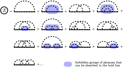
Figure 13: Forbidden and allowed self-energy bold diagrams up to third order

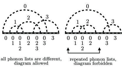
Figure 14: Algorithm to check if a self-energy diagram is allowed in BDMC. Each phonon is assigned a unique number and each propagator has a list of phonons covering it. Diagrams with each list being unique are allowed, and diagrams with repeated lists are forbidden.

References

- (1) D. J. J. Marchand, G. De Filippis, V. Cataudella, M. Berciu, N. Nagaosa, N. V. Prokof’ev, A. S. Mishchenko, and P. C. E. Stamp, Phys. Rev. Lett. 105, 266605, (2010).
- (2) T. Holstein, Ann. Phys. (NY) 8, 325 (1959); ibid Ann. Phys. (NY) 8, 343 (1959).
- (3) W. P. Su, J. R. Schrieffer, and A. J. Heeger, Phys. Rev. Lett. 42, 1698 (1979).
- (4) A. J. Heeger, S. Kivelson, J. R. Schrieffer, and W. P. Su, Rev. Mod. Phys. 60, 781 (1988).
- (5) S. Barisić, J. Labbé, and J. Friedel, Phys. Rev. Lett. 25, 919 (1970)
- (6) S. Barisić, Phys. Rev. B 5, 932 (1972); ibid, Phys. Rev. B 5, 941 (1972).
- (7) H. Fröhlich, Adv. Phys. 3, 325 (1954).
- (8) S.I. Pekar, E.I. Rashba, and V.I. Sheka, Zh. Eksp. Teor. Fiz. 76 251 (1979) [Sov. Phys. JETP 49, 129 (1979)]; I.M. Dykman and S.I. Pekar, Dokl. Akad. Nauk SSSR 83, 825 (1952).
- (9) C. Slezak, A. Macridin, G. A. Sawatzky, M. Jarrell, and T. A. Maier Phys. Rev. B 73, 205122, 2006; Bayo Lau, Mona Berciu, and George A. Sawatzky Phys. Rev. B 76, 174305 (2007).
- (10) G. D. Mahan, Many-Particle Physics (Plenum, New York, 1981).
- (11) I. G. Lang and Y. A. Firsov, JETP 16, 1301, (1963).
- (12) L.D. Landau, Phys. Zh. Sowjet. 3, 664 (1933); L.D. Landau, S.I. Pekar, ZhETF 18, 419 (1948). See also S.I. Pekar, ZhETF 17, 1868 (1947); ibid 18, 105 (1948).
- (13) Y. Toyozawa, Prog. Theor. Phys. 26, 29 (1961).
- (14) R.P. Feynman, Phys. Rev. 97, 660 (1955); R.P. Feynman et al, Phys. Rev. 127, 1004 (1962)
- (15) S. Ciuchi, F. de Pasquale, S. Fratini, and D. Feinberg, Phys. Rev. B 56, 4494 (1997).
- (16) M. Berciu, Phys. Rev. Lett. 97, 036402 (2006); G. L. Goodvin, M. Berciu, and G. A. Sawatzky, Phys. Rev. B 74, 245104 (2006).
- (17) M. Berciu and G. L. Goodvin, Phys. Rev. B 76, 165109 (2007).
- (18) G. L. Goodvin and M. Berciu, Phys. Rev. B 78, 235120 (2008).
- (19) E. Jeckelmann and S.R. White, Phys. Rev. B 57, 6376 (1998); R. Bulla, T. Costi and T. Pruschke, Rev. Mod. Phys. 80, 395 (2008); H. Fehske, S.A. Trugman, in Polarons in Advanced Materials, ed. by A.S. Alexandrov (Canopus/Springer, Bristol, 2007); J. T. Devreese and A. S. Alexandrov, Rep. Prog. Phys. 72, 066501 (2009).
- (20) B. Gerlach and H. Löwen, Rev. Mod. Phys. 63, 63 (1991).
- (21) M.J. Rice, Phys. Lett. 71, 152 (1979); E.J. Mele, M.J. Rice, Phys. Rev. Lett. 45, 926 (1980).
- (22) V.M. Stojanović, P.A. Bobbert and M.A.J.Michels, Phys. Rev. B 69, 144302 (2004); K. Hannewald, V.M. Stojanović, J.M.T Schellekens, P.A. Bobbert, G. Kresse and J. Hafner, Phys. Rev. B 69, 075211 (2004).
- (23) V. Cataudella, G. De Filippis, and C. A. Perroni Phys. Rev. B 83, 165203 (2011); C. A. Perroni, V. Marigliano Ramaglia, and V. Cataudella, Phys. Rev. B 84, 014303 (2011); C. A. Perroni and V. Cataudella, Phys. Rev. B 85, 155205 (2012).
- (24) T.-M. Wu, D.W Brown and K. Lindenberg, Phys. Rev. B 47, 10122 (1993); K.S. Song and R.T. Williams, Self-Trapped Excitons (Springer-Verlag, Berlin, 1996); M. Pope and C.E. Swenberg, Electronic Processes in Organic Crystals and Polymers, (Oxford University Press, Oxford, 1999).
- (25) S. M. Weber-Milbrodt, J. T. Gammel, A. R. Bishop, and E. Y. Loh, Jr., Phys. Rev. B 45, 6435 (1992); H. Roder, A. R. Bishop, and J. T. Gammel, Phys. Rev. Lett. 70, 3498 (1993); M. Yu. Lavrentiev, H. Koppel, and L. S. Cederbaum, Phys. Rev. B 51, 5790(1995); H. Fehske, M. Kinateder, G. Wellein, and A. R. Bishop, Phys. Rev. B 63, 245121 (2001); S. L. Dexheimer, Coherent Vibrational Dynamics of Exciton Self-Trapping in Quasi-One-Dimensional Systems, chapter 6 of S. De Silvestri, G. Cerullo, G. Lanzani, eds., Coherent Vibrational Dynamics, (Taylor and Francis Applied Spectroscopy Series, 2008).
- (26) T.P. Devereaux, T. Cuk, Z.-X. Shen and N. Nagaosa, Phys. Rev. Lett. 93, 117004 (2004).
- (27) J. Sun, Y. Zhao and W. Liang, Phys. Rev. B 79, 155112 (2009).
- (28) Q. Liu, Y. Zhao, W. Wang, and T. Kato, Phys. Rev. B 79, 165105 (2009).
- (29) M. Capone, W. Stephan, and M. Grilli, Phys. Rev. B 56, 4484 (1997).
- (30) M. Zoli, Phys. Rev. B 66 012303 (2002).
- (31) C. J. Chandler and F. Marsiglio Phys. Rev. B 90, 245149 (2014).
- (32) Y. Zhao, P. Zanardi and G. Chen, Phys. Rev. B 70, 195113 (2004).
- (33) V.M. Stojanović and M. Vanević, Phys. Rev. B 78, 214301 (2008).
- (34) N. V. Prokof’ev, B. V. Svistunov and I. S. Tupitsyn, JETP 87, 310 (1998).
- (35) G. De Filippis, V. Cataudella, A. S. Mishchenko, C. A. Perroni, and N. Nagaosa, Phys. Rev. B 80, 195104 (2009).
- (36) For the Frölich polaron see: G. Whitfield and R. Puff, Phys. Rev. 139, A338 (1965); D.M. Larsen, Phys. Rev. 144, 697 (1966); and Ref. PhysRevLett.81.2514, above.
- (37) M. Berciu and H. Fehske, Phys. Rev. B 82, 085116 (2010).
- (38) F. Herrera, K. W. Madison, R. V. Krems and M. Berciu, Phys. Rev. Lett. 110, 223002 (2013).
- (39) O. S. Barisić, Phys. Rev. Lett. 98, 209701 (2007); M. Berciu, Phys. Rev. Lett. 98, 209702 (2007).
- (40) A. Alvermann, D. M. Edwards, and H. Fehske, Phys. Rev. Lett. 98, 056602 (2007).
- (41) N. V. Prokof’ev, and B. V. Svistunov, Phys. Rev. Lett. 99, 250201 (2007).
- (42) N. V. Prokof’ev, and B. V. Svistunov, Phys. Rev. B 77, 020408 (2008).
- (43) N. V. Prokof’ev, and B. V. Svistunov, Phys. Rev. B 77, 125101 (2008).
- (44) N. V. Prokof’ev and B. V. Svistunov, Phys. Rev. Lett. 81, 2514 (1998).
- (45) A. S. Mishchenko, N. V. Prokof’ev, A. Sakamoto, and B. V. Svistunov, Phys. Rev. B 62, 6317(2000).
- (46) A. Macridin, Ph.D. thesis, Rijkuniversiteit Gröningen, 2003.
- (47) A. S. Mishchenko, N. V. Prokof’ev, and B. V. Svistunov, Phys. Rev. B64, 033101 (2001).
- (48) A. S. Mishchenko, N. Nagaosa, and N. Prokof’ev Phys. Rev. Lett. 113, 166402 (2014).
- (49) A. Alvermann, H. Fehske, and S. A. Trugman, Phys. Rev. B 81, 165113 (2010).
- (50) It is important that in the DQMC and BDMC methods, calculations are done over a finite time interval, which is roughly equivalent to introducing an IR cut-off. If this were not done, then high-order terms in the perturbation series would eventually dominate - the series is of course divergent - and the series would ’blow up’ at high orders. At finite time , a factor more than compensates for the number of diagrams containing phonon lines.
- (51) M. Chakraborty, N. Mohanta, A. Taraphder, B. I. Min, and H. Fehske Phys. Rev. B 93, 155130 (2016).
- (52) M. Berciu and H. Fehske, Phys. Rev. B 84, 165104 (2011); H. Ebrahimnejad, G. A. Sawatzky and M. Berciu, J. Phys.: Cond. Mat. 28, 105603 (2016).
- (53) S. A. Trugman, Phys. Rev. B 37, 1597 (1988).
- (54) C. P. J. Adolphs and M. Berciu, Europhys. Lett. 102, 47003 (2013).
- (55) S. Li and S. Johnston, Europhys. Lett. 109, 27007 (2015); S. Li, E. A. Nowadnick, and S. Johnston, Phys. Rev. B 92, 064301 (2015).
- (56) A. Troisi, Adv. Mat. 19, 2000 (2007).
- (57) F. Herrera and R. V. Krems, Phys. Rev. A 84, 051401(R) (2011).
- (58) L. D. Carr, D. DeMille, R. V. Krems, and J. Ye, New J. Phys. 11, (2009).
- (59) J. Doyle, B. Friedrich, R. V. Krems and F. Masnou-Seeuws, Euro. J. Phys. D 31, 149 (2004).