Event-triggered second-moment stabilization of linear systems under packet drops

Abstract

This paper deals with the stabilization of linear systems with process noise under packet drops between the sensor and the controller. Our aim is to ensure exponential convergence of the second moment of the plant state to a given bound in finite time. Motivated by considerations about the efficient use of the available resources, we adopt an event-triggering approach to design the transmission policy. In our design, the sensor’s decision to transmit or not the state to the controller is based on an online evaluation of the future satisfaction of the control objective. The resulting event-triggering policy is hence specifically tailored to the control objective. We formally establish that the proposed event-triggering policy meets the desired objective and quantify its efficiency by providing an upper bound on the fraction of expected number of transmissions in an infinite time interval. Simulations for scalar and vector systems illustrate the results.

I Introduction

One of the fundamental abstractions of cyber-physical systems is the idea of networked control systems, the main characteristic feature of which is that feedback signals are communicated over a communication channel or network. As a result, control must be performed under communication constraints such as quantization, unreliability, and latency. These limitations make it necessary to design control systems that tune the use of the available resources to the desired level of task performance. With this goal in mind, this paper explores the design of event-triggered transmission policies for second-moment stabilization of linear plants under packet drops.

Literature review

The increasing deployment of cyberphysical systems has brought to the forefront the need for systematic design methodologies that integrate control, communication, and computation instead of independently designing these components and integrating them in an adhoc manner, see e.g. [2, 3]. Among this growing body of literature, the contents of this paper are particularly related to works that deal with feedback control under communication constraints, see [4, 5, 6] and references therein, and specifically packet drops or erasure channels, see e.g., [7, 8, 9]. In the past decade, opportunistic state-triggered control methods [10, 11, 12], have gained popularity for designing transmission policies for networked control systems that seek to efficiently use the communication resources. The main idea behind this approach is to design state-dependent triggering criteria that opportunistically specify when certain actions (updating the actuation signal, sampling data, or communicating information) must be executed. More generally, the triggering criteria may also depend on the desired control objective, and the available information about the state, communication channel, and other constraints. In the context of the communication service, the emphasis has largely been on minimizing the number of transmissions rather than the quantized data, often ignoring the limits imposed by channel characteristics, with some notable exceptions, see [13, 14, 15, 16, 17] and references therein. In our previous work [18, 19], we have also sought to address these limitations for deterministic models of the behavior of the communication channel. Although today there exists a large body of work on opportunistic state-triggered control, the application of these ideas in the stochastic setting is still relatively limited. This is despite the fact that one of the first works on event-triggered control [20] was in this setting. Event-triggering methods in the stochastic setting have almost exclusively been utilized in finite or infinite horizon optimal control problems with fixed threshold-based triggering. The works [21, 22, 23] also incorporate transmission costs in the cost function and analyze the optimal transmission costs. On the other hand, [24, 25] analyze the transmission rates. In addition, [23, 24, 25, 26] also consider packet drops. The work [27] shows optimality of certainty equivalence in event-triggered control for certain finite horizon problems. In contrast to starting with an event-triggered control policy, the work [28] formulates an optimal control problem over a finite horizon with the constraint that at most a smaller number of transmissions may occur, and the optimal control policy turns out to be event-triggered. Finally, we should remark that stochastic stability, in the sense of moment stability, with event-triggered control has received much less attention. The work [29] follows [10] to study self-triggered sampling for second-moment stability of state-feedback controlled stochastic differential equations. The work [30] proposes a fixed threshold-based event-triggered anytime control policy under packet drops. It assumes that the controller has knowledge of the transmission times, including when a packet is dropped, and the policy guarantees second-moment stability with exponential convergence to a finite bound asymptotically. Both [29, 30] are applicable to multi-dimensional nonlinear systems.

Statement of contributions

We formulate the problem of second-moment stabilization of scalar linear systems subject to process noise and independent identically distributed packet drops in the communication channel. Our goal is to design a policy to prescribe transmissions from the sensor to the controller that ensures exponential convergence in finite time of the second moment of the plant state to an ultimate bound. Our first contribution is the design of an event-triggered transmission policy in which the decision to transmit or not is determined by a state-based criterion that uses the available information. The synthesis of our policy is based on a two-step design procedure. First, we consider a nominal quasi-time-triggered policy where no transmission occurs for a given number of timesteps, and then transmissions occur on every time step thereafter. Second, we define the event-trigger policy by evaluating the expectation of the system performance at the next reception time given the current information under the nominal policy, and prescribe a transmission if this expectation fails to meet the objective. This approach results in a transmission policy more complex than a threshold-based triggering, but since it is driven by the control objective results in fewer transmissions. Our second contribution is the rigorous characterization of the system evolution, first under the proposed family of nominal transmission policies and second, building on this analysis, under the proposed event-triggered transmission policy. This helps us identify sufficient conditions on the ultimate bound, the system parameters, and the communication channel that guarantee that the event-triggered policy indeed meets the control objective. Our third contribution compares the efficiency of the proposed design with respect to time-triggered policies and provides an upper bound on the fraction of the expected number of transmissions over an infinite time horizon. Our fourth and last contribution is the extension of our exponential convergence guarantees to the vector case and a discussion of the design and analysis challenges in extending the characterization of efficiency. Various simulations illustrate our results. We omit the proofs that appeared in the conference version [1] of this work and instead refer the interested reader there.

Notation

We let $\mathbb{R}$, $\mathbb{R}_{\geq 0}$, ${\mathbb{Z}}$, ${\mathbb{N}}$, ${\mathbb{N}}_{0}$ denote the set of real, non-negative real numbers, integers, positive integers and non-negative integers respectively. We use the notation $[a,b]_{\mathbb{Z}}$ and $(a,b)_{\mathbb{Z}}$ to denote $[a,b]\operatorname{\cap}{\mathbb{Z}}$ and $(a,b)\operatorname{\cap}{\mathbb{Z}}$, respectively. We use similar notation for half-open/half-closed intervals. For a matrix $A$, we let $\text{tr}(A)$ denote the trace of the matrix. Given a set $A$, we denote its indicator function by $\mathbf{1}_{A}$, i.e., $\mathbf{1}_{A}(x)=0$ if $x\notin A$ and $\mathbf{1}_{A}(x)=1$ if $x\in A$. We use ‘w.p.’ as a shorthand for ‘with probability’. We denote the expectation given a transmission policy $\mathcal{P}$ as $\mathbb{E}_{\mathcal{P}}\left[.\right]$. Let $(\Omega,\mathcal{F},P)$ be a probability space and $\mathcal{G}_{1}\subset\mathcal{G}_{2}\subset\mathcal{F}$ be two sub-sigma fields of $\mathcal{F}$. Then, the tower property of conditional expectation is

$$\mathbb{E}\left[\mathbb{E}\left[X\ |\ \mathcal{G}_{2}\right]\ |\ \mathcal{G}_{1}\right]=\mathbb{E}\left[X\ |\ \mathcal{G}_{1}\right]=\mathbb{E}\left[\mathbb{E}\left[X\ |\ \mathcal{G}_{1}\right]\ |\ \mathcal{G}_{2}\right].$$

II Problem statement

This section describes the model for the plant dynamics and the assumptions on the sensor, actuator, and the communication channel between them. Given this setup, we then specify the objective for the control design.

Plant, sensor, and actuator

Consider a scalar discrete-time linear time-invariant system evolving according to

$$x_{k+1}=ax_{k}+u_{k}+v_{k},$$ (1)

for $k\in{\mathbb{N}}_{0}$. Here $x\in\mathbb{R}$ denotes the state of the plant, $a\in\mathbb{R}$ defines the system internal dynamics, $u\in\mathbb{R}$ is the control input, and $v$ is a zero-mean independent and identically distributed process noise with covariance $M>0$, uncorrelated with the system state.

A sensor measures the plant state $x_{k}$ at time $k$. The sensor, being not co-located with the controller, communicates with it over an unreliable communication channel. The sensor maintains an estimate of the plant state given the ‘history’ (defined precisely below) up to time $k-1$. During the time between two successful communications, the controller itself estimates the plant state. We let $\hat{x}_{k}^{+}$ be the controller’s estimate of the plant state $x_{k}$ given the past history of transmissions and receptions including those at time $k$, if any. This results in a control action given by $u_{k}=L\hat{x}_{k}^{+}$. We assume that the sensor can independently compute $\hat{x}_{k}^{+}$ at the next time step $k+1$ for each $k\in{\mathbb{N}}_{0}$ (this is possible with acknowledgments from the controller to the sensor on successful reception times). We denote the sensor estimation error and controller estimation error as $e_{k}\triangleq x_{k}-\hat{x}_{k}$ and $e_{k}^{+}\triangleq x_{k}-\hat{x}_{k}^{+}$, which are known to the sensor at all times, but not to the controller.

Communication channel

The sensor can transmit the plant state to the controller with infinite precision and instantaneously at time steps of its choosing, but packets might be lost. We define the transmission process $\{t_{k}\}_{k\in{\mathbb{N}}_{0}}$ as

$$t_{k}\triangleq\begin{cases}1,\quad\text{if a packet is transmitted at }k,\\ 0,\quad\text{if no packet is transmitted at }k.\end{cases}$$ (2)

The way in which this process occurs is determined by a transmission policy $\mathcal{T}$, to be specified by the designer. Similarly, we define a reception process $\{r_{k}\}_{k\in{\mathbb{N}}_{0}}$, with $r_{k}$ being $1$ or $0$ depending on whether a packet is received or not at $k$. The transmission and reception processes may differ due to Bernoulli-distributed packet drops. Formally, if $p\in(0,1]$ denotes the probability of successful transmission, the reception process is

$$r_{k}\triangleq\begin{cases}1,\quad\text{w.p. }p\text{ if }t_{k}=1,\\ 0,\quad\text{if }t_{k}=0\text{ or w.p. }(1-p)\text{ if }t_{k}=1.\end{cases}$$ (3)

We denote the latest reception time before $k$ and latest reception time up to $k$ by $R_{k}$ and $R_{k}^{+}$, resp. Formally,

$$R_{k} \triangleq\max\{i<k:r_{i}=1\},$$ (4a)

$$R_{k}^{+} \triangleq\max\{i\leq k:r_{i}=1\}.$$ (4b)

Both times coincide if $r_{k}=0$. The need for separate notions would become clearer later: the notion of $R_{k}$ plays a role in the design of the triggering rule, while the notion of $R_{k}^{+}$ is useful in the analysis of the system evolution. We denote the sequence of all (successful) reception times as $\{S_{j}\}_{j\in{\mathbb{N}}_{0}}$, i.e.,

$$S_{0}=0,\quad S_{j+1}\triangleq\min\{k>S_{j}:r_{k}=1\},$$ (5)

where we have assumed, without loss of generality, that $S_{0}=0$ and hence also $r_{0}=1$. Thus, $S_{j}$ is the $j^{\text{th}}$ reception time.

System evolution

Given the sensor-controller communication model specified above, we describe the system evolution and the controller’s estimate, respectively, as

$$x_{k+1} =ax_{k}+L\hat{x}_{k}^{+}+v_{k}=\bar{a}x_{k}-Le_{k}^{+}+v_{k},$$ (6a)

$$\hat{x}_{k+1} =\bar{a}\hat{x}_{k}^{+},$$ (6b)

where $$\bar{a}=a+L$$ and

$$\hat{x}_{k}^{+}\triangleq\begin{cases}\hat{x}_{k}\quad&\text{if }r_{k}=0,\\ x_{k},\quad&\text{if }r_{k}=1.\end{cases}$$ (6c)

The use of $\hat{x}^{+}$ and $e^{+}$ is motivated by our goal of designing a state-triggered transmission policy: the decision to transmit at time $k$ is made by the sensor based on $x_{k}$ and $\hat{x}_{k}$ (or equivalently $e_{k}$), while the plant state at $k+1$ depends on whether a packet is received or not at $k$, which is captured by $\hat{x}^{+}$ and $e_{k}^{+}$. We denote by $I_{k}\triangleq(k,x_{k},e_{k},R_{k},x_{R_{k}})$ the information available to the sensor at time $k$, based on which it decides whether to transmit or not. We also let $I_{k}^{+}\triangleq(k,x_{k},e_{k}^{+},R_{k}^{+},x_{R_{k}^{+}})$ be the information available at the controller at time $k$, which can also be independently computed by the sensor at the end of time step $k$ upon receiving or not receiving an acknowledgment. Note that $I_{k}^{+}$ differs from $I_{k}$ only if $k$ is a reception time, i.e., $r_{k}=1$ (equivalently, only if $k=S_{j}$ for some $j$). The closed-loop system is not fully defined until a transmission policy $\mathcal{T}$, determining the transmission process (2), is specified. This specification is guided by the control objective detailed next.

Control objective

Our objective is to ensure the stability of the plant dynamics with a guaranteed level of performance. We rely on stochastic stability because the presence of random disturbances and the unreliable communication channel make the plant evolution stochastic. Formally, we seek to synthesize a transmission policy $\mathcal{T}$ ensuring

$$\mathbb{E}_{\mathcal{T}}\left[x_{k}^{2}\ |\ I_{0}^{+}\right]\leq\max\{c^{2k}x_{0}^{2},B\},\quad\forall k\in{\mathbb{N}},$$ (7)

which corresponds to the second moment of the plant state, conditioned on the initial information, converging at an exponential rate $c\in(0,1)$ to its ultimate bound $B\geq 0$.

A possible, purely time-triggered transmission policy to guarantee (7) would be to transmit at every time instant. Such policy would presumably lead to an inefficient use of the communication channel, since it is oblivious to the plant state in making decisions about transmissions. Instead, we seek to design an event-triggered transmission policy $\mathcal{T}$, i.e., an online policy in which the decision to transmit or not is determined by a state-based criterion that uses the available information.

Standing assumptions

We assume the drift constant $a$ is such that $|a|>1$, so that control is necessary. We also assume $\bar{a}^{2}<c^{2}<1$, so that the performance function is always non-positive under zero noise and no packet drops. Finally, we assume $a^{2}(1-p)<1$. This latter condition is necessary for second-moment stabilizability under Bernoulli packet drops, see e.g. [31, 32]. In our discussion, the condition is necessary for the convergence of certain infinite series (we come back to this point in Remark IV.2). For the reader’s reference, we present in the appendix a list of the symbols most frequently used along the paper.

III Event-triggered transmission policy

This section provides an alternative control objective and shows that its satisfaction implies the original one defined in Section II is also satisfied. This reformulated objective serves then as the basis for our design of the event-triggered transmission policy.

III-A Online control objective

The control objective stated in (7) prescribes, given the initial condition, a property on the whole system trajectory in a priori fashion. This ‘open-loop’ nature makes it challenging to address the design of the transmission policy. To tackle this, we describe here an alternative control objective which prescribes a property on the system trajectory in an online fashion, making it more handleable for design, and whose satisfaction implies the original objective is also met. To this end, consider the performance function,

$$h_{k}=x_{k}^{2}-\max\{c^{2(k-R_{k})}x_{R_{k}}^{2},B\},$$ (8)

which has the interpretation of capturing the desired performance at time $k$ with respect to the state at the latest reception time before $k$. Given this interpretation, consider the alternative control objective that consists of ensuring that

$$\mathbb{E}_{\mathcal{T}}\left[h_{k}\ |\ I_{R_{k}}^{+}\right]\leq 0,\quad\forall k\in{\mathbb{N}}.$$ (9)

The next result shows that the satisfaction of (9) ensures that the original control objective (7) is also met. The proof relies on the use of induction and can be found in [1].

Lemma III.1.

(The online control objective is stronger than the original control objective [1]). If a transmission policy $\mathcal{T}$ ensures the online objective (9), then it also guarantees the control objective (7).

Given this result, our strategy for control design is to satisfy the stronger but easier to handle online control objective (9) rather than working directly with the original objective (7).

III-B Two-step design strategy: nominal and event-triggered transmission policies

In this section, we introduce our event-triggered design strategy to meet the control objective. Before giving a full description, we first detail the design principle we have adopted to approach the problem. Later, we discuss how our two-step design strategy corresponds to this design principle.

• [Design principle:] The fundamental principle of event-triggered control is to assess if it is necessary to transmit at the current time given the control objective and the available information about the system and its state (for example, for deterministic discrete-time systems with a perfect channel, a transmission may be triggered at time $k$ only if $h_{k+1}$ would be greater than $0$ in the absence of a transmission). If the channel is not perfect, then its properties must also be taken into consideration when deciding whether to transmit or not (for example, if the channel induces time delays bounded by $\gamma$, then $h_{k+\gamma}$ must be checked in the absence of a transmission at time $k$). In order to implement this same basic principle for the problem at hand, one needs to address the challenges presented by the Bernoulli packet drops and the goal of stochastic stability with a strict convergence rate requirement (as specified in (9)). A key observation in this regard is the fact that it is not possible to assess the necessity of transmission at a given time $k$ independently of future actions, as the occurrence of the next (random) reception time is determined by not only the current action but also the future actions. This motivates our two-step design strategy. We assess the necessity of transmission using a nominal transmission policy in which there is no transmission at the current time $k$. Our actual transmission policy at that time is then based on the expected performance under this nominal transmission policy: if the nominal transmission policy deems it ‘not necessary’ to transmit on time $k$, meaning that the performance objective is expected to be met under it, then indeed we do not transmit on time $k$.

We next describe our design of the event-triggered transmission policy. The key idea is the belief that, in the absence of reception of packets, the likelihood of violating the performance criterion must increase with time. We refer to this as the monotonicity property. Therefore, we design a transmission policy that overtly seeks to satisfy the performance criterion (9) only at the next (random) reception time in order to guarantee that the performance objective is not violated at any time step. Later, our analysis will show that the monotonicity property above does indeed hold.

We seek to design an event-triggered policy $\mathcal{T}$ ensuring

$$\mathbb{E}_{\mathcal{T}}\left[h_{S_{j+1}}\ |\ I_{S_{j}}^{+}\right]\leq 0,\quad\text{ for each }j\in{\mathbb{N}}_{0}.$$

In general, computing the conditional expectation for an arbitrary event-triggered transmission policy $\mathcal{T}$ is challenging. This is because the evolution of the system state between consecutive reception times depends on the transmission instants, which are in turn determined online by the triggering function of the state and the specific realizations of the noise and the packet drops. Therefore, we take the two-step strategy described above: first, we consider a family of nominal quasi-time-triggered transmission policies $\mathcal{T}_{k}^{D}$, for which we can compute $\mathbb{E}_{\mathcal{T}_{k}^{D}}\left[h_{R_{k+1}}\ |\ I_{k}\right]$; then, we use this expectation under the nominal policy to design the event-triggered policy.

We start by defining a family of nominal transmission policies indexed by $k\in{\mathbb{N}}_{0}$ as

$$\mathcal{T}_{k}^{D}:t_{i}=\begin{cases}0,\quad i\in\{k,\ldots,k+D-1\},\\ 1,\quad i\geq k+D,\end{cases}$$ (10)

where $D\geq 1$. Under this nominal policy, no transmissions occur for the first $D$ time steps from $k$ to $k+D-1$, and transmissions occur on every time step thereafter ($D$ is therefore the length of the interval from time $k$ during which no transmissions occur). With the nominal policy, we associate the following look-ahead criterion,

$$G_{k}^{D} \triangleq\mathbb{E}_{\mathcal{T}_{k}^{D}}\left[h_{R_{k+1}}\ |\ I_{k}\right]$$ (11)

$$=\sum_{s=D}^{\infty}\mathbb{E}\left[h_{R_{k+1}}\ |\ I_{k},R_{k+1}=k+s\right](1-p)^{s-D}p,$$

which is the conditional expectation of the performance function at the next reception time, given the information at $k$ under the transmission policy $\mathcal{T}_{k}^{D}$. This interpretation gives rise to the central idea behind our event-triggered transmission policy: if the criterion is positive (i.e., the performance objective is expected to be violated at the next reception time if no transmission occurs for $D$ timesteps, and forever after), then we need to start transmitting earlier to try to revert the situation before it is too late. Formally, the event-triggered policy $\mathcal{T}_{\mathcal{E}}$, given the last successful reception time $R_{k}=S_{j}$, is

$$\mathcal{T}_{\mathcal{E}}:t_{k}=\begin{cases}0,\quad\text{if }k\in\{R_{k}+1,\ldots,F_{k}-1\}\\ 1,\quad\text{if }k\in\{F_{k},\ldots,S_{j+1}\},\end{cases}$$ (12a)

where

$$F_{k}\triangleq\min\{\ell>R_{k}:G_{\ell}^{D}\geq 0\}.$$ (12b)

Thus, under the proposed policy, the sensor transmits on each time step starting at $F_{k}$ (the first time after $R_{k}=S_{j}$ when the look-ahead criterion is positive) until a successful reception occurs at $S_{j+1}$, for each $j\in{\mathbb{N}}_{0}$. The complete transmission policy is then obtained recursively. In the course of the paper, we analyze the system under the transmission policy (12), with respect to an arbitrary reception time $S_{j}$. Thus, it is convenient to also introduce the notation

$$T_{j}\triangleq\min\{\ell>S_{j}:G_{\ell}^{D}\geq 0\},$$ (13)

which is the first time after $S_{j}$ when a transmission occurs.

Remark III.2.

(Interpretation of the parameter $D$). The interpretation of the role of the parameter $D$ depends on the context. In the nominal policy $\mathcal{T}_{k}^{D}$, $D$ has the role of idle duration from $k$ during which no transmissions occur. In the actual event-triggered transmission policy (12), $D$ has the role of look-ahead horizon. Specifically, given the information available to the sensor at time $k$, the sign of the look-ahead function $G_{k}^{D}$ answers the question of whether the sensor could afford not to transmit for the next $D$ time steps and still meet the control objective. If at a time $k$, $G_{k}^{D}<0$, then the sensor can afford not to transmit on time steps $\{k,\ldots,k+D-1\}$, as there exists a transmission sequence in future, given by the nominal policy, that would satisfy the control objective. Thus, at a particular time $k$ when $G_{k}^{D}<0$, $D$ may be interpreted as a lower bound on the time-to-go for a required transmission. Hence, intuitively we can see that, in the actual transmission policy (12), a larger value of $D$ makes the policy more conservative, because it requires a longer guaranteed no-transmission horizon. $\bullet$

Remark III.3.

(Special case of deterministic channel). It is interesting to look at the transmission policy (12) in the special case of a deterministic channel, i.e., no packet drops ($p=1$). Observe from (11) that in this case, $G_{k}^{D}=\mathbb{E}\left[h_{k+D}\ |\ I_{k}\right]$. If additionally there were no process noise, then this further simplifies to $G_{k}^{D}=h_{k+D}$. Then, the policy (12) reduces to

$$t_{k}=\begin{cases}1,\quad\text{if }G_{k}^{D}\geq 0\\ 0,\quad\text{if }G_{k}^{D}<0,\end{cases}$$

which is a commonly used event-triggering policy for control over deterministic channels, see e.g., [18]. Thus, the proposed policy (12) is a natural generalization of the basic principle of event-triggering to control over channels with probabilistic packet drops. $\bullet$

IV Analysis of the system evolution under the nominal policy

Here, we characterize the evolution of the system when operating under the nominal transmission policy. This characterization is key later to help us provide performance guarantees of the event-triggered transmission policy.

IV-A Performance evaluation functions and their properties

The following result provides a useful closed-form expression of the look-ahead criterion $G_{k}^{D}$ as a function of $I_{k}$. Its proof appears in [1].

Lemma IV.1.

(Closed-form expression for the look-ahead function [1]). The look-ahead function is well defined and takes the form

$$G_{k}^{D} =p\Big{[}g_{D}(\bar{a}^{2})x_{k}^{2}+2\big{(}g_{D}(a\bar{a})-g_{D}(\bar{a}^{2})\big{)}x_{k}e_{k}$$

$$\quad+\big{(}g_{D}(a^{2})-2g_{D}(a\bar{a})+g_{D}(\bar{a}^{2})\big{)}e_{k}^{2}$$

$$\quad+\mkern 1.5mu\overline{\mkern-1.5muM\mkern-1.5mu}\mkern 1.5mu\left(g_{D}(a^{2})-\frac{1}{p}\right)-g_{D}(c^{2})z_{k}$$

$$\quad-\Big{(}\frac{B}{p}-c^{2q_{k}^{D}}g_{D}(c^{2})z_{k}\Big{)}(1-p)^{q_{k}^{D}}\Big{]},$$

where

$$\mkern-20.0mug_{D}(b) \triangleq\frac{b^{D}}{1-b(1-p)},\ \ \mkern 1.5mu\overline{\mkern-1.5muM\mkern-1.5mu}\mkern 1.5mu\triangleq\frac{M}{a^{2}-1},\ \ z_{k}\triangleq c^{2(k-R_{k})}x_{R_{k}}^{2},$$

$$q_{k}^{D} \triangleq\max\left\{0,\left\lceil\frac{\log\left(\frac{x_{R_{k}}^{2}}{B}\right)}{\log(1/c^{2})}\right\rceil-(k-R_{k})-D\right\}.$$ (14)

The function $G_{k}^{D}$ helps determine whether or not to transmit at time $k$. However, to analyze the evolution of the performance function $h_{k}$ between successive reception times $S_{j}$ and $S_{j+1}$, we introduce the performance-evaluation function,

$$J_{k}^{D} \triangleq\mathbb{E}_{\mathcal{T}_{k}^{D}}\left[h_{R_{k+1}^{+}}\ |\ I_{k}^{+}\right]$$ (15)

$$=\sum_{s=D}^{\infty}\mathbb{E}\left[h_{R_{k+1}^{+}}\ |\ I_{k}^{+},R_{k+1}=k+s\right](1-p)^{s-D}p.$$

Note the similarity with the definition of $G_{k}^{D}$ (with the exception that $J_{k}^{D}$ is conditioned upon the information $I_{k}^{+}$). Observe that $J_{k}^{D}\neq G_{k}^{D}$ only if $k=S_{j}$ for some $j$. Hence we focus on $J_{S_{j}}^{D}$ for $j\in{\mathbb{N}}_{0}$,

$$J_{S_{j}}^{D}=\sum_{s=D}^{\infty}H(s,x_{S_{j}}^{2})(1-p)^{s-D}p,$$ (16)

where

$$H(s,x_{S_{j}}^{2})\triangleq\mathbb{E}\left[h_{S_{j}+s}\ |\ I_{S_{j}}^{+},S_{j}+s\leq S_{j+1}\right],$$ (17)

which we call the open-loop performance evolution function. This function describes the evolution of the expected value of the performance function in open loop, during the inter-reception times, conditioned upon $I_{S_{j}}^{+}$, the information available at the last reception time upon reception.

Remark IV.2.

(Necessary condition for second-moment stability). The condition $a^{2}(1-p)<1$, which we assumed in the standing assumption in Section II, is necessary for the convergence of the series (11) and (16), which define the look-ahead criterion and performance-evaluation function, respectively. This can be seen from the proofs of Lemma IV.1 and Lemma IV.3, in [1]. The necessity of the condition $a^{2}(1-p)<1$ for second-moment stability can also be derived from the information-theoretic or data-rate arguments employed in [31, 32]. $\bullet$

The next result gives closed-form expressions for the performance-evaluation function $J_{S_{j}}^{D}$ and the open-loop performance evaluation function $H$. The proof appears in [1].

Lemma IV.3.

(Closed-form expressions for the performance-evaluation and the open-loop performance evaluation functions [1]). The performance-evaluation function is well defined and takes the form

$$J_{S_{j}}^{D} =p\Big{[}g_{D}(\bar{a}^{2})x_{S_{j}}^{2}+\mkern 1.5mu\overline{\mkern-1.5muM\mkern-1.5mu}\mkern 1.5mu\left(g_{D}(a^{2})-\frac{1}{p}\right)-g_{D}(c^{2})x_{S_{j}}^{2}$$

$$\quad-\Big{(}\frac{B}{p}-c^{2w_{k}^{D}}g_{D}(c^{2})x_{S_{j}}^{2}\Big{)}(1-p)^{w_{S_{j}}^{D}}\Big{]},$$

where $g_{D}$ is defined in (14) and

$$w_{S_{j}}^{D} \triangleq\max\left\{0,\left\lceil\frac{\log\left(\frac{x_{S_{j}}^{2}}{B}\right)}{\log(1/c^{2})}\right\rceil-D\right\}.$$ (18)

The open-loop performance evaluation function takes the form

$$H(s,y)=\bar{a}^{2s}y+\mkern 1.5mu\overline{\mkern-1.5muM\mkern-1.5mu}\mkern 1.5mu(a^{2s}-1)-\max\{c^{2s}y,B\}.$$ (19)

The next result specifies some useful properties of the look-ahead $G_{k}^{D}$ and the performance-evaluation $J_{k}^{D}$ functions. The proof appears in [1].

Proposition IV.4.

(Properties of the look-ahead and performance-evaluation functions [1]). For $D\in{\mathbb{N}}$, under the same hypotheses as in Proposition IV.6, the following hold:

• Let $\mathcal{T}$ be any transmission policy. Then, for any $k\in{\mathbb{N}}_{0}$,

  $$\mathbb{E}_{\mathcal{T}}\left[G_{k+1}^{D}\ |\ I_{k},r_{k}=0\right]=G_{k}^{D+1},$$

  $$\mathbb{E}_{\mathcal{T}}\left[G_{k+1}^{D}\ |\ I_{k},r_{k}=1\right]=J_{k}^{D+1}.$$

• For $\mathcal{D}\in{\mathbb{N}}$, define

  $$\mkern-10.0mu\mathcal{G}(\mathcal{D})\triangleq\left(g_{\mathcal{D}}(\bar{a}^{2})-g_{\mathcal{D}}(c^{2})\right)\frac{B}{c^{2\mathcal{D}}}+\mkern 1.5mu\overline{\mkern-1.5muM\mkern-1.5mu}\mkern 1.5mu\left(g_{\mathcal{D}}(a^{2})-\frac{1}{p}\right).$$ (20)

  If $\mathcal{G}(\mathcal{D})<0$, then $J_{S_{j}}^{\mathcal{D}}<0$, for any $j\in{\mathbb{N}}_{0}$.

• Suppose the hypothesis of (b) is true. Then, for $d\in\{1,\ldots,\mathcal{D}\}$ and for any $j\in{\mathbb{N}}_{0}$, $J_{S_{j}}^{d}\leq J_{S_{j}}^{d+1}$.

The value of the function $\mathcal{G}$ (defined in (20)) at $D$ has the interpretation of being a uniform (over the plant state space) upper bound on $J_{S_{j}}^{D}$, the expectation of the open-loop performance function at the next (random) reception time. The condition $\mathcal{G}(D)<0$ can be interpreted as establishing a lower bound on the value of $B$, the ultimate bound, as a function of the system and communication channel parameters. The next result establishes a useful property of $\mathcal{G}$ which would be useful in our forthcoming analysis.

Lemma IV.5.

(The function $\mathcal{G}$ is strictly increasing). Under the hypotheses of Proposition IV.6, the function $\mathcal{G}$ (cf. (20)) is strictly increasing on $[0,\infty)$.

Proof.

The derivative of $\mathcal{G}$ with respect to $\mathcal{D}$ is

$$\frac{\mathrm{d}\mathcal{G}}{\mathrm{d}\mathcal{D}} =\mkern 1.5mu\overline{\mkern-1.5muM\mkern-1.5mu}\mkern 1.5mu\log(a^{2})\frac{a^{2\mathcal{D}}}{1-a^{2}(1-p)}-B\log\left(\frac{c^{2}}{\bar{a}^{2}}\right)\frac{\bar{a}^{2\mathcal{D}}}{1-\bar{a}^{2}(1-p)}$$

$$<B\log\left(\frac{c^{2}}{\bar{a}^{2}}\right)\left[\frac{a^{2\mathcal{D}}}{1-a^{2}(1-p)}-\frac{(\bar{a}/c)^{2\mathcal{D}}}{1-\bar{a}^{2}(1-p)}\right],$$

where the inequality follows from the assumption that $B>B^{*}$ and (21). Then, observe that for $\mathcal{D}\geq 0$

$$a^{2\mathcal{D}}(1-\bar{a}^{2}(1-p))-(\bar{a}/c)^{2\mathcal{D}}(1-a^{2}(1-p))$$

$$>(a^{2\mathcal{D}}-(\bar{a}/c)^{2\mathcal{D}})(1-a^{2}(1-p))>0,$$

where the inequalities follow form the fact $\bar{a}^{2}<c^{2}<a^{2}$. Thus, $\frac{\mathrm{d}\mathcal{G}}{\mathrm{d}\mathcal{D}}>0$ for $\mathcal{D}\geq 0$. ∎

IV-B Monotonicity of the open-loop performance function

This section establishes the monotonicity of the open-loop performance function $H$, which forms the basis for our main results. Recall from our discussion in Section III-B that this property refers to the intuition that, in the absence of reception of packets, the likelihood of violating the performance criterion must increase with time. This property is captured by the following result.

Proposition IV.6.

(Monotonicity of the open-loop performance function). There exists

$$B^{*}>B_{c}\triangleq\mkern 1.5mu\overline{\mkern-1.5muM\mkern-1.5mu}\mkern 1.5mu\frac{\log(a^{2})}{\log\left(\frac{c^{2}}{\bar{a}^{2}}\right)}>0$$ (21)

such that if $B>B^{*}$ then for each $y\in\mathbb{R}_{\geq 0}$, the function $H(.,y)$ has the property:

$$H(s_{1},y)>0\implies H(s_{2},y)>0,\quad\forall s_{2}\geq s_{1}.$$ (22)

Proposition IV.6 states that, given the plant state is $y$ at any reception time $S_{j}$, then there is a time $s_{0}$ such that, in the absence of receptions, the plant state is expected to satisfy the performance criterion (9) until $S_{j}+s_{0}$ and violate it on every time step thereafter.

The proof of Proposition IV.6 requires a number of intermediate results that we detail next. We start by introducing the functions $f_{1},f_{2}:\mathbb{R}_{\geq 0}^{2}\rightarrow\mathbb{R}$,

$$f_{1}(s,y) \triangleq\bar{a}^{2s}y+\mkern 1.5mu\overline{\mkern-1.5muM\mkern-1.5mu}\mkern 1.5mu(a^{2s}-1)-c^{2s}y,$$ (23a)

$$f_{2}(s,y) \triangleq\bar{a}^{2s}y+\mkern 1.5mu\overline{\mkern-1.5muM\mkern-1.5mu}\mkern 1.5mu(a^{2s}-1)-B.$$ (23b)

Notice, from (19), that $H(s,y)=\min\{f_{1}(s,y),f_{2}(s,y)\}$.

(a) Case-I

(b) Case-II

(c) Case-III

(d) Case-IV

Figure 1: For $y>B$, there are four possible cases of how $f_{1}(.,y)$ and $f_{2}(.,y)$ and hence $H(.,y)$ evolve. In the figures, $\CIRCLE$ and $\blacksquare$ show the points $(s_{*},F_{*})$ and $(s_{**},F_{**})$, respectively. In Case-I $s_{*}(y)<s_{**}(y)$ and in Cases II-IV $s_{*}(y)\geq s_{**}(y)$. In addition, in Case-II $F_{**}(y)\leq 0$, in Case-III $F_{**}(y)>0$ and $F_{*}(y)>0$ and in Case-IV $F_{**}(y)>0$ and $F_{*}(y)\leq 0$.

Our proof strategy to establish Proposition IV.6 is the following:

Roadmap: We first show that $f_{2}(.,y)$ is strongly convex and $f_{1}(.,y)$ is quasiconvex. Notice that for $y\leq B$, $H(s,y)=f_{2}(s,y)$ for all $s\geq 0$. Thus for $y>B$, we analyze the conditions under which one or the other of the functions $f_{1}(.,y)$ and $f_{2}(.,y)$ is the minimum of the two. In this process, we find it useful to analyze the relationship between $s_{*}$ and $s_{**}$, the unique point where $f_{1}(.,y)$ attains its minimum and the unique point where $f_{1}(.,y)$ equals $f_{2}(.,y)$, respectively. In addition, the function values at these points

$$F_{*}(y) \triangleq f_{2}(s_{*}(y),y)$$ (24a)

$$F_{**}(y) \triangleq f_{1}(s_{**}(y),y)=f_{2}(s_{**}(y),y),$$ (24b)

also play an important role. Based on the relationship between $(s_{*},F_{*})$ and $(s_{**},F_{**})$, the behavior of the open-loop performance function, for $y>B$, can be qualitatively classified into four different cases, which are illustrated in Figure 1. Notice from the plots that $H$ has the property (22) in all but Case-IV. Thus, the key to the proof is in showing that Case-IV does not occur under the hypothesis of Proposition IV.6.

In the sequel, we discuss the various claims alluded to in the above roadmap.

Lemma IV.7.

(Convexity properties of $f_{2}$). For any fixed $y\in\mathbb{R}_{\geq 0}$, the function $f_{2}(.,y)$ is strongly convex.

Proof.

Strong convexity of $f_{2}$ with respect to $s$ for a fixed $y$ follows directly by taking the second derivative.

$$\frac{\partial^{2}f_{2}}{\partial s^{2}}=\bar{a}^{2s}\log^{2}(\bar{a}^{2})y+\mkern 1.5mu\overline{\mkern-1.5muM\mkern-1.5mu}\mkern 1.5mua^{2s}\log^{2}(a^{2})>\mkern 1.5mu\overline{\mkern-1.5muM\mkern-1.5mu}\mkern 1.5mu\log^{2}(a^{2})>0.$$

∎

On the other hand, $f_{1}(.,y)$ for any fixed $y\in\mathbb{R}_{\geq 0}$ is only quasiconvex in general, as the following result states.

Lemma IV.8.

(Convexity properties of $f_{1}$). For any fixed $y\in\mathbb{R}_{\geq 0}$, the function $f_{1}(.,y)$ is quasiconvex.

Proof.

For any fixed $y\in\mathbb{R}_{\geq 0}$, let $g_{1}(s)\triangleq f_{1}(s,y)$. Then,

$$g^{\prime}_{1}(s)=\bar{a}^{2s}y\log(\bar{a}^{2})+\mkern 1.5mu\overline{\mkern-1.5muM\mkern-1.5mu}\mkern 1.5mua^{2s}\log(a^{2})-c^{2s}y\log(c^{2}).$$

Notice that $g^{\prime}_{1}(s)$ has the same sign as

$$g_{2}(s) \triangleq\frac{g^{\prime}_{1}(s)}{\bar{a}^{2s}}$$

$$=y\log(\bar{a}^{2})+\mkern 1.5mu\overline{\mkern-1.5muM\mkern-1.5mu}\mkern 1.5mu\left(\frac{a}{\bar{a}}\right)^{2s}\log(a^{2})-\left(\frac{c}{\bar{a}}\right)^{2s}y\log(c^{2}),$$

which, by the standing assumptions, is a strictly increasing function of $s$. Since $g^{\prime}_{1}(s)$ has the same sign as $g_{2}(s)$, we conclude that $g_{1}=f_{1}(.,y)$ is quasiconvex. ∎

The strong convexity of $f_{2}(.,y)$ and quasiconvexity of $f_{1}(.,y)$ are very useful in proving Proposition IV.6. In order to proceed with the proof, we need to determine the subsets of the domain where the minimum in the definition of $H$ is achieved by each of the functions $f_{1}$ and $f_{2}$. Thus, we define the function

$$s_{**}(y)\triangleq\frac{\log(y)-\log(B)}{\log(1/c^{2})},$$ (25)

that corresponds to the point where $f_{1}$ and $f_{2}$ cross each other, i.e., $H(s_{**}(y),y)=f_{1}(s_{**}(y),y)=f_{2}(s_{**}(y),y)$.

Lemma IV.9.

(Convexity properties of $H$). Given any $y\in\mathbb{R}_{\geq 0}$, $H(.,y)$ is quasiconvex on $[0,s_{**}(y)]$ and strongly convex on $[s_{**}(y),\infty)$.

Proof.

The result follows directly from the definition (25) of $s_{**}(y)$, the facts that

$$H(s,y) =f_{1}(s,y)<f_{2}(s,y),\quad\forall s\in[0,s_{**}(y)),$$

$$H(s,y) =f_{2}(s,y)<f_{1}(s,y),\quad\forall s\in(s_{**}(y),\infty),$$

together with the quasiconvexity of $f_{1}(.,y)$, cf. Lemma IV.8, and the strong convexity of $f_{2}(.,y)$, cf. Lemma IV.7. ∎

Note that, by itself, this result is not sufficient to ascertain the convexity properties of $H(.,y)$ over the whole domain $\mathbb{R}_{\geq 0}$. However, if $f_{2}(.,y)$ is increasing for $s>s_{**}(y)$, then Lemma IV.9 would imply that $H(.,y)$ is quasiconvex on $\mathbb{R}_{\geq 0}$, and this together with the fact that $H(0,y)=0$, in turn imply that the property (22) holds. Thus, our next objective is to find the values of $y$ for which $f_{2}(.,y)$ is increasing for $s>s_{**}(y)$. To this aim, we find the minimizer of this function as

$$s_{*}(y)\triangleq\log\left(\frac{y\log\left(\frac{1}{\bar{a}^{2}}\right)}{\mkern 1.5mu\overline{\mkern-1.5muM\mkern-1.5mu}\mkern 1.5mu\log(a^{2})}\right)\frac{1}{\log\left(\frac{a^{2}}{\bar{a}^{2}}\right)}.$$ (26)

Clearly, if $s_{*}(y)\leq s_{**}(y)$, then $f_{2}(.,y)$ would be increasing for $s>s_{**}(y)$, as desired. Therefore, we are interested in the function

$$W(y)\triangleq s_{*}(y)-s_{**}(y),$$ (27)

and, more specifically, on the sign of $W$ as a function of $y$.

Lemma IV.10.

(Monotonic behavior of $W$). The function $W$ is monotonically decreasing on $[B,\infty)$ and $W(U)=0$, where $U$ is given by

$$\log(U)\triangleq\frac{\log\left(\frac{B\log\left(\frac{1}{\bar{a}^{2}}\right)}{\mkern 1.5mu\overline{\mkern-1.5muM\mkern-1.5mu}\mkern 1.5mu\log(a^{2})}\right)\log\left(\frac{1}{c^{2}}\right)}{\log\left(\frac{a^{2}c^{2}}{\bar{a}^{2}}\right)}+\log(B).$$ (28)

Proof.

From (25) and (26), we see that

$$W^{\prime}(y) =\left(\frac{1}{\log\left(\frac{a^{2}}{\bar{a}^{2}}\right)}-\frac{1}{\log\left(\frac{1}{c^{2}}\right)}\right)\frac{1}{y}=\frac{-\log\left(\frac{a^{2}c^{2}}{\bar{a}^{2}}\right)}{\log\left(\frac{a^{2}}{\bar{a}^{2}}\right)\log\left(\frac{1}{c^{2}}\right)y}<0,$$

where the last inequality follows from the fact that $a^{2}>1$ and $c^{2}>\bar{a}^{2}$ and the fact that $y\in[B,\infty)$. Thus, $W$ is monotonically decreasing for $y\in[B,\infty)$. The value of $U$ can be obtained directly by solving $W(U)=0$. ∎

It is clear that if $F_{*}(y)$, the minimum value of $f_{2}(.,y)$, (see (24a)) is greater than zero then again property (22) is satisfied. Thus, we now note how $F_{*}(y)$ evolves with $y$.

Lemma IV.11.

(Motonic behavior of $F_{*}$). The function $F_{*}$ is monotonically increasing on $\mathbb{R}_{>0}$.

Proof.

It can be easily verified that

$$F_{*}^{\prime}(y)=\left(\bar{a}^{2s_{*}(y)}+\frac{\mkern 1.5mu\overline{\mkern-1.5muM\mkern-1.5mu}\mkern 1.5mua^{2s_{*}(y)}}{y}\right)\frac{\log(a^{2})}{\log\left(\frac{a^{2}}{\bar{a}^{2}}\right)}>0,$$

which proves the result. ∎

Now, also note that, if $H(s_{**}(y),y)\leq 0$, then strong convexity of $H(.,y)$ in the interval $[s_{**}(y),\infty)$ guarantees the property (22). Thus, we now analyze the evolution of the function $F_{**}(y)$ (see (24b)) with $y$.

Lemma IV.12.

(Convexity properties of $F_{**}$). The function $F_{**}$ is quasiconvex on $\mathbb{R}_{\geq 0}$.

Proof.

We can easily verify that

$$F_{**}^{\prime}(y)=\left(\bar{a}^{2s_{**}(y)}\log\left(\frac{\bar{a}^{2}}{c^{2}}\right)+\frac{\mkern 1.5mu\overline{\mkern-1.5muM\mkern-1.5mu}\mkern 1.5mua^{2s_{**}(y)}\log(a^{2})}{y}\right)\frac{1}{\log\left(\frac{1}{c^{2}}\right)},$$

which has the same sign as the function $g(y)\triangleq F_{**}^{\prime}(y)/\bar{a}^{2s_{**}(y)}$. We can then verify, for all $y>0$,

$$g^{\prime}(y)=\frac{\mkern 1.5mu\overline{\mkern-1.5muM\mkern-1.5mu}\mkern 1.5mu\left(\frac{a^{2}}{\bar{a}^{2}}\right)^{s_{**}(y)}\log(a^{2})\log\left(\frac{a^{2}c^{2}}{\bar{a}^{2}}\right)}{\log^{2}\left(\frac{1}{c^{2}}\right)y^{2}}>0.$$

Thus, $g$ is strictly increasing, and since $g(y)$ and $F_{**}^{\prime}(y)$ have the same sign, $F_{**}$ is quasiconvex. ∎

Lemma IV.13.

(Choice of $B$). There exists $B^{*}>0$ such that $F_{**}(U(B^{*}))=0$ and, if $B>B^{*}$, then $F_{**}(U(B))<0$.

Proof.

We first make explicit the dependence of $U$ on $B$ by rewriting (28) as

$$\log(U(B))=\frac{P_{1}}{P_{2}}\log(B)+\frac{P_{3}P_{4}}{P_{2}},$$ (29)

where

$$P_{1}\triangleq\log\left(\frac{a^{2}}{\bar{a}^{2}}\right),\quad P_{2}\triangleq\log\left(\frac{a^{2}c^{2}}{\bar{a}^{2}}\right),$$

$$P_{3}\triangleq\log\left(\frac{1}{c^{2}}\right),\quad P_{4}\triangleq\log\left(\frac{\log\left(\frac{1}{\bar{a}^{2}}\right)}{\mkern 1.5mu\overline{\mkern-1.5muM\mkern-1.5mu}\mkern 1.5mu\log(a^{2})}\right).$$

Note that

$$U(B)=e^{\frac{P_{3}P_{4}}{P_{2}}}\cdot B^{\frac{P_{1}}{P_{2}}},\quad\frac{\mathrm{d}U}{\mathrm{d}B}=\frac{P_{1}U}{P_{2}B}.$$

Using the definitions of $P_{1}$, $P_{2}$, and $P_{3}$ in (25), we obtain

$$s_{**}(U(B))=\frac{\log(B)}{P_{2}}+\frac{P_{4}}{P_{2}}.$$

Next, we use this expression to evaluate (24b) and establish $F_{**}(U(B))=Y(B)-\mkern 1.5mu\overline{\mkern-1.5muM\mkern-1.5mu}\mkern 1.5mu-B$, where

$$Y(B)\triangleq\bar{a}^{2s_{**}(U(B))}U(B)+\mkern 1.5mu\overline{\mkern-1.5muM\mkern-1.5mu}\mkern 1.5mua^{2s_{**}(U(B))}.$$

One can then verify, using the definition of $P_{1}$ and $P_{2}$ to simplify the expressions, that

$$\frac{\mathrm{d}F_{**}(U(B))}{\mathrm{d}B}=\frac{Y(B)\log(a^{2})}{P_{2}B}-1,$$

$$\frac{\mathrm{d}^{2}F_{**}(U(B))}{\mathrm{d}B^{2}}=-\frac{Y(B)\log(a^{2})\log\left(\frac{c^{2}}{\bar{a}^{2}}\right)}{P_{2}^{2}B^{2}}<0,\ \forall B>0.$$

Thus, the function $F_{**}(U(.))$ is a strictly concave function - it has at most two zeros and it is positive only between those zeros, if they exist. Now, note that for $B_{0}=e^{-P_{4}}$, $s_{**}(U(B_{0}))=0$ and hence $F_{**}(U(B_{0}))=0$. Therefore, there exists a $B^{*}\geq B_{0}$ such that $F_{**}(U(B^{*}))=0$ and by the strict concavity of $F_{**}(U(.))$, $F_{**}(U(B))$ is strictly decreasing for all $B\geq B^{*}$. This proves the result. ∎

The final arguments of the proof also suggest a method to numerically find $B^{*}$. First, note that $B_{0}<B_{c}$. As a result, if $F_{**}(U(.))$ is non-increasing at $B_{0}$ then $B^{*}=B_{c}$. Otherwise, the other zero, $B_{z}$ of $F_{**}(U(.))$ can be found by simply marching forward in $B$ from $B_{0}$. Then, $B^{*}=\max\{B_{c},B_{z}\}$. Now, all the pieces necessary for the proof of Proposition IV.6 are finally in place.

Proof of Proposition IV.6.

First, notice from the definition (25) of $s_{**}$ that if $y\leq B$, then $H(s,y)=f_{2}(s,y)$ for all $s\geq 0$. Then, the strong convexity of $f_{2}(.,y)$, cf. Lemma IV.7, and the fact that $f_{2}(0,y)\leq 0$ for all $y\leq B$ are sufficient to prove Proposition IV.6. Therefore, in what follows, we assume that $y>B$.

There are four possible cases that may arise, specified as

Case-I: $$s_{*}(y)<s_{**}(y),$$

Case-II: $$s_{*}(y)\geq s_{**}(y)\land F_{**}(y)\leq 0,$$

Case-III: $$s_{*}(y)\geq s_{**}(y)\land F_{**}(y)>0\land F_{*}(y)>0,$$

Case-IV: $$s_{*}(y)\geq s_{**}(y)\land F_{**}(y)>0\land F_{*}(y)\leq 0.$$

Figure 1 illustrates each of these cases. First, note that for $y>B$, $H(0,y)=0$. Also, recall from Lemma IV.9 that $H(.,y)$ is quasiconvex for $s\in[0,s_{**}(y)]$ and thus in this interval, $H$ satisfies the property (22). It is only the behavior of $H(s,y)$ for $s\in[s_{**}(y),\infty)$ that is of concern to us.

Thus in Case-I, since $s_{*}(y)<s_{**}(y)$ and the strong convexity of $f_{2}(.,y)$, cf. Lemma IV.7, mean that $H(.,y)$ is strictly increasing in $[s_{**}(y),\infty)$, which is sufficient to prove property (22). In Case-II, $F_{**}(y)\leq 0$ and again the strong convexity of $H(.,y)$ in $[s_{**}(y),\infty)$ guarantees the result. In Case-III, the fact that $F_{*}(y)>0$ directly guarantees property (22).

It is only in Case IV when the property (22) would be violated. So, now we take into account the assumption that $B>B^{*}$. Notice from (27) and Lemma IV.10 that in Case IV, $y\in[B,U]$. Also notice that $F_{**}(B)=0$ and by Lemma IV.13 that $F_{**}(U)<0$. Then, the quasiconvexity of $F_{**}$, cf. Lemma IV.12, implies that $F_{**}(y)\leq 0$ for all $y\in[B,U]$, which ensures that Case IV does not occur. This completes the proof of Proposition IV.6. ∎

Observe that, in ruling out the occurrence of Case-IV we have also ruled out the occurrence of Case-III. From Lemma IV.13, we see that the condition $B>B^{*}$ is only sufficient and it may seem that the ‘good’ Case-III has been ruled out inadvertently. However, note that, by the definitions of $F_{*}$ and $F_{**}$, $F_{**}(y)\geq F_{*}(y)$ for any $y>0$. Thus, Case-IV is ruled out only if both $F_{**}(y)$ and $F_{*}(y)$ are of the same sign for all $y\in[B,U]$. Therefore, ruling out Case-IV automatically also rules out Case-III.

V Convergence and performance analysis under the event-triggered policy

In this section, we characterize the convergence and performance properties of the system evolution operating under the event-triggered transmission policy $\mathcal{T}_{\mathcal{E}}$ defined in (12).

V-A Convergence guarantees: the control objective is achieved

The following statement is the main result of the paper and shows that the control objective is achieved by the proposed event-triggered transmission policy.

Theorem V.1.

(The event-triggered policy meets the control objective). If the ultimate bound satisfies $B>B^{*}$ and $D\in{\mathbb{N}}$ is such that $\mathcal{G}(D)<0$, cf. (20), then the event-triggered policy $\mathcal{T}_{\mathcal{E}}$ guarantees that $\mathbb{E}_{\mathcal{T}_{\mathcal{E}}}\left[h_{k}\ |\ I_{R_{k}}^{+}\right]\leq 0$ for all $k\in{\mathbb{N}}$.

Proof.

We structure the proof around the following two claims.

Claim (a): For any $j\in{\mathbb{N}}$, $\mathbb{E}_{\mathcal{T}_{\mathcal{E}}}\left[h_{S_{j+1}}\ |\ I_{S_{j}}^{+}\right]\leq 0$ implies $\mathbb{E}_{\mathcal{T}_{\mathcal{E}}}\left[h_{k}\ |\ I_{S_{j}}^{+}\right]\leq 0$ for all $k\in[S_{j},S_{j+1}]_{\mathbb{Z}}$.

Claim (b): For any $j\in{\mathbb{N}}$, $\mathbb{E}_{\mathcal{T}_{\mathcal{E}}}\left[h_{S_{j+1}}\ |\ I_{S_{j}}^{+}\right]<0$.

Note that if both the claims hold, the result automatically follows. Therefore, it now suffices to establish claims (a) and (b). Towards this aim, first observe that

$$\mathbb{E}_{\mathcal{T}_{\mathcal{E}}}\left[h_{k}\ |\ I_{S_{j}}^{+}\right]=\mathbb{E}\left[h_{k}\ |\ I_{S_{j}}^{+}\right],\quad\forall k\in[S_{j},S_{j+1}]_{\mathbb{Z}}.$$

This can be reasoned by noting that a transmission policy only affects the sequence of reception times, $\{S_{j}\}_{j\in{\mathbb{N}}}$, and has otherwise no effect on the evolution of the performance function $h_{k}$ during the inter-reception times. Hence, from the definition (17) of $H$, it follows that

$$\mathbb{E}_{\mathcal{T}_{\mathcal{E}}}\left[h_{k}\ |\ I_{S_{j}}^{+}\right]=H(k-S_{j},x_{S_{j}}^{2}),\quad\forall k\in[S_{j},S_{j+1}]_{\mathbb{Z}}.$$

Consequently, Proposition IV.6 implies claim (a).

Next, we prove claim (b). From Proposition IV.4(a), we see that for all $k\in(S_{j},S_{j+1})_{\mathbb{Z}}$,

$$\mathbb{E}_{\mathcal{T}_{\mathcal{E}}}\left[G_{k+1}^{D}\ |\ I_{S_{j}}^{+}\right] =\mathbb{E}_{\mathcal{T}_{\mathcal{E}}}\left[\mathbb{E}_{\mathcal{T}_{\mathcal{E}}}\left[G_{k+1}^{D}\ |\ I_{k},r_{k}=0\right]\ |\ I_{S_{j}}^{+}\right]$$

$$=\mathbb{E}_{\mathcal{T}_{\mathcal{E}}}\left[G_{k}^{D+1}\ |\ I_{S_{j}}^{+}\right],$$ (30)

and

$$\mathbb{E}_{\mathcal{T}_{\mathcal{E}}}\left[G_{S_{j}+1}^{D}\ |\ I_{S_{j}}^{+}\right] =\mathbb{E}_{\mathcal{T}_{\mathcal{E}}}\left[G_{S_{j}+1}^{D}\ |\ I_{S_{j}},r_{S_{j}}=1\right]=J_{S_{j}}^{D+1}.$$ (31)

Then, under the policy $\mathcal{T}_{\mathcal{E}}$, and using (13),

$$\mathbb{E}_{\mathcal{T}_{\mathcal{E}}}\left[h_{S_{j+1}}\ |\ I_{S_{j}}^{+}\right] =\mathbb{E}_{\mathcal{T}_{\mathcal{E}}}\left[\mathbb{E}_{\mathcal{T}_{\mathcal{E}}}\left[h_{S_{j+1}}\ |\ I_{T_{j}}\right]\ |\ I_{S_{j}}^{+}\right]$$

$$=\mathbb{E}_{\mathcal{T}_{\mathcal{E}}}\left[\mathbb{E}_{\mathcal{T}_{T_{j}}^{0}}\left[h_{S_{j+1}}\ |\ I_{T_{j}}\right]\ |\ I_{S_{j}}^{+}\right]$$

$$=\mathbb{E}_{\mathcal{T}_{\mathcal{E}}}\left[G_{T_{j}}^{0}\ |\ I_{S_{j}}^{+}\right],$$

where we have first used the ‘Tower property’ of conditional expectation, then the definition of the event-triggered policy (12a) and finally the definition of $G_{T_{j}}^{0}$. Using (30) and (31) recursively, this expression reduces to

$$\mathbb{E}_{\mathcal{T}_{\mathcal{E}}}\left[h_{S_{j+1}}\ |\ I_{S_{j}}^{+}\right]$$

$$=\begin{cases}J_{S_{j}}^{T_{j}-S_{j}},\quad&\text{if }T_{j}\leq S_{j}+D\\ \mathbb{E}_{\mathcal{T}_{\mathcal{E}}}\left[G_{T_{j}-D}^{D}\ |\ I_{S_{j}}^{+}\right],\quad&\text{if }T_{j}>S_{j}+D.\end{cases}$$

In the case when $T_{j}\leq S_{j}+D$, claims (b) and (c) of Proposition IV.4 imply that $J_{S_{j}}^{T_{j}-S_{j}}<0$. Also note that, under the policy $\mathcal{T}_{\mathcal{E}}$, $G_{k}^{D}<0$ for all $k\in(S_{j},T_{j})_{\mathbb{Z}}$. Thus, in the case when $T_{j}>S_{j}+D$, we have $G_{T_{j}-D}^{D}<0$. Thus, we have shown that claim (b) is true, which completes the proof. ∎

A consequence of Theorem V.1 along with Lemma III.1 is that the event-triggered policy $\mathcal{T}_{\mathcal{E}}$ guarantees

$$\mathbb{E}_{\mathcal{T}_{\mathcal{E}}}\left[x_{k}^{2}\ |\ I_{0}^{+}\right]\leq\max\{c^{2k}x_{0}^{2},B\},\quad\forall k\in{\mathbb{N}}_{0},$$

the original control objective. In other words, the proposed event-triggered transmission policy guarantees that the expected value of $x_{k}^{2}$ converges at an exponential rate to its ultimate bound of $B$.

Remark V.2.

(Sufficient conditions impose lower bounds on the ultimate bound). The two conditions identified in Theorem V.1 to ensure the satisfaction of the control objective may be interpreted as lower bounds on the choice of the ultimate bound $B$. The first condition, $B>B^{*}$, comes from Proposition IV.6 and ensures the monotonicity property of the open-loop performance function $H$. Thus, as expected, we see from (21) that $B^{*}$ does not depend on the channel properties, namely the packet-drop probability $(1-p)$, or the look-ahead horizon $D$. On the other hand, the second condition, $\mathcal{G}(D)<0$, imposes a lower bound on $B$ which does have a dependence on both parameters $p$ and $D$. This condition can be rewritten as

$$\left(g_{D}(c^{2})-g_{D}(\bar{a}^{2})\right)\frac{B}{c^{2D}}>\mkern 1.5mu\overline{\mkern-1.5muM\mkern-1.5mu}\mkern 1.5mu\left(g_{D}(a^{2})-g_{D}(1)\right).$$ (32)

Comparing this inequality with (21), we see that there is a strong resemblance between the two. In fact, if in (32) the function $g_{D}$ were replaced with $\log$ and the factor $c^{2D}$ removed, we would get (21). This is not unexpected because $\mathcal{G}(D)$ is a uniform (over the plant state space) upper bound on $J_{S_{j}}^{D}$, which is nothing but the expectation of the open-loop performance function at the next (random) reception time. $\bullet$

The next result shows that if the event-triggered transmission policy meets the control objective for a certain look-ahead horizon, then it also meets it for any other shorter look-ahead horizon.

Corollary V.3.

(If $\mathcal{T}_{\mathcal{E}}$ meets the control objective with parameter $D$ then it also does with a smaller $D$). Let $B>B^{*}$ and $D\in{\mathbb{N}}$ such that $\mathcal{G}(D)<0$. Then, for any $D^{\prime}<D$, the event-triggered transmission policy $\mathcal{T}_{\mathcal{E}}$ with parameter $D^{\prime}$ meets the control objective.

Proof.

For $D^{\prime}<D$, Corollary IV.5 guarantees that $\mathcal{G}(D^{\prime})<\mathcal{G}(D)$. Therefore, $\mathcal{G}(D)<0$ implies that $\mathcal{G}(D^{\prime})<0$. Thus, according to Theorem V.1, the event-triggered transmission policy (12) with parameter $D^{\prime}$ ensures the control objective is met. ∎

Note that this result is aligned with Remark III.2 where we made the observation that, intuitively, a larger $D$ in the event-triggered transmission policy (12) is more conservative. It is also interesting to observe that, as a result of Corollary V.3, if $\mathcal{G}(D)<0$ is satisfied for $D>1$, then the control objective is met with $D=1$, which corresponds to a time-triggered policy that transmits at every time step (i.e., has period $T=1$).

V-B Performance guarantees: benefits over time-triggering

Here we analyze the efficiency of the proposed event-triggered transmission policy in terms of the fraction of the number of time steps at which transmissions occur. For any stopping time $K$, we introduce the expected transmission fraction

$$\mathcal{F}_{0}^{K}\triangleq\frac{\mathbb{E}_{\mathcal{T}_{\mathcal{E}}}\left[\displaystyle\sum_{k=1}^{K}\mathbf{1}_{\{t_{k}=1\}}\ |\ I_{0}^{+}\right]}{\mathbb{E}_{\mathcal{T}_{\mathcal{E}}}\left[K\ |\ I_{0}^{+}\right]}.$$ (33)

This corresponds to the expected fraction of time steps from $1$ to $K$ at which transmissions occur. Note that $K$ might be a random variable itself, which justifies the expectation operation taken in the denominator. The following result provides an upper bound on this expected transmission fraction.

Proposition V.4.

(Upper bound on the expected transmission fraction). Suppose that $\mathcal{G}(D+\mathcal{B})<0$ (see (20)), where $D$ is the parameter in the event-triggered transmission policy (12) and $\mathcal{B}\in{\mathbb{N}}_{0}$. Then

$$\mathcal{F}_{0}^{\infty}\leq\frac{1}{1+\mathcal{B}p}.$$

Proof.

Given Corollary V.3, the remainder of the proof relies on finding an upper bound on the expected transmission fraction in a cycle from one reception time to the next, i.e., $\mathcal{F}_{S_{j}}^{S_{j+1}}$ and then extending it to obtain the running transmission fraction $\mathcal{F}_{0}^{S_{N}}$ for an arbitrary $N\in{\mathbb{N}}$. Note that, in any such cycle, the channel is idle, i.e., $t_{k}=0$, for $k$ from $S_{j}+1$ to $T_{j}-1$ and transmissions occur from $T_{j}$ to $S_{j+1}$.

Now, observe that the assumption that (20) is satisfied with $D+\mathcal{B}$ in place of $D$ implies, according to Proposition IV.4(b), that $J_{S_{j}}^{D+\mathcal{B}}<0$ for all $j\in{\mathbb{N}}_{0}$. We also know from (30) and (31) that

$$\mathbb{E}_{\mathcal{T}_{\mathcal{E}}}\left[G_{S_{j}+\mathcal{B}}^{D}\ |\ I_{S_{j}}^{+}\right]=\mathbb{E}_{\mathcal{T}_{\mathcal{E}}}\left[J_{S_{j}}^{D+\mathcal{B}}\ |\ I_{S_{j}}^{+}\right]<0,$$

which means that $T_{j}-1\geq S_{j}+\mathcal{B}$. Thus,

$$\mathbb{E}_{\mathcal{T}_{\mathcal{E}}}\left[\displaystyle\sum_{k=S_{j}+1}^{S_{j+1}}\mathbf{1}_{\{t_{k}=0\}}\ |\ I_{S_{j}}^{+}\right] =\mathbb{E}_{\mathcal{T}_{\mathcal{E}}}\left[T_{j}-1-S_{j}\ |\ I_{S_{j}}^{+}\right]\geq\mathcal{B}.$$

On the other hand, since the probability of $S_{j+1}-T_{j}+1$ being $1$ is $p$, being $2$ is $(1-p)p$, and so on, we note that

$$\mathbb{E}_{\mathcal{T}_{\mathcal{E}}}\left[\displaystyle\sum_{k=S_{j}+1}^{S_{j+1}}\mathbf{1}_{\{t_{k}=1\}}\ |\ I_{S_{j}}^{+}\right] =\mathbb{E}_{\mathcal{T}_{\mathcal{E}}}\left[S_{j+1}-T_{j}+1\ |\ I_{S_{j}}^{+}\right]$$

$$=p\sum_{s=0}^{\infty}(s+1)(1-p)^{s}=\frac{1}{p}.$$

We can extend this reasoning further to $N$ cycles, from $S_{0}=0$ to $S_{N}$, to obtain

$$\mathbb{E}_{\mathcal{T}_{\mathcal{E}}}\left[\displaystyle\sum_{k=1}^{S_{N}}\mathbf{1}_{\{t_{k}=0\}}\ |\ I_{S_{j}}^{+}\right]\geq N\mathcal{B},$$

$$\mathbb{E}_{\mathcal{T}_{\mathcal{E}}}\left[\displaystyle\sum_{k=1}^{S_{N}}\mathbf{1}_{\{t_{k}=1\}}\ |\ I_{S_{j}}^{+}\right]=\frac{N}{p}.$$

Finally, note that

$$\mathbb{E}_{\mathcal{T}_{\mathcal{E}}}\left[S_{N}\ |\ I_{0}^{+}\right]$$

$$=\mathbb{E}_{\mathcal{T}_{\mathcal{E}}}\left[\displaystyle\sum_{k=1}^{S_{N}}\mathbf{1}_{\{t_{k}=0\}}\ |\ I_{0}^{+}\right]+\mathbb{E}_{\mathcal{T}_{\mathcal{E}}}\left[\displaystyle\sum_{k=1}^{S_{N}}\mathbf{1}_{\{t_{k}=1\}}\ |\ I_{0}^{+}\right].$$

Then using (33), this yields an upper bound on the expected transmission fraction during $[0,S_{N}]_{\mathbb{Z}}$

$$\mathcal{F}_{0}^{S_{N}}\leq\frac{1}{1+\mathcal{B}p},$$

which we see is independent of $N$. The result then follows by taking the limit as $N\rightarrow\infty$. ∎

An expected transmission fraction of $1$ corresponds to a transmission occurring at every time step almost surely, i.e., essentially a time-triggered policy. Therefore, Proposition V.4 states that the number of transmissions under the event-triggered policy $\mathcal{T}_{\mathcal{E}}$ is guaranteed to be less than that of a time-triggered policy.

Remark V.5.

(Interpretation of the parameter $D$-cont’d). Proposition V.4 is consistent with our intuition, cf. Remark III.2, that a larger $D$ in the event-triggered transmission policy (12) is more conservative. In fact, if $D_{1}<D_{2}$ and $D_{1}+\mathcal{B}_{1}=D_{2}+\mathcal{B}_{2}$, then $\mathcal{B}_{1}>\mathcal{B}_{2}$ and thus the upper bound on the expected transmission fraction is larger for larger $D$. Note that since Proposition V.4 is only a statement about the upper bound on the expected transmission fraction, we do not formally claim that larger $D$ is more conservative. In fact, different control parameters lead to different state trajectories and thus, formally, we can only say that larger $D$ is more conservative at each point in state space (corresponding to the initial condition for each trajectory). However, Remark III.2, Corollary V.3, Proposition V.4 and the simulation results in the sequel together suggest that, starting from the same initial conditions, a larger $D$ has a larger expected transmission fraction. $\bullet$

Remark V.6.

(Optimal sufficient periodic transmission policy). Under the assumptions of Proposition V.4, we know that the time-triggered policy with period $T=1$ satisfies the control objective. It is conceivable that a time-triggered transmission policy with period $T>1$ (i.e., with transmission fraction $1/T<1$) also achieves it. To see this, consider the open-loop performance evolution function (19) at integer multiples of $T$, i.e., $H(sT,y)$ and (20). Then, a time-triggered transmission policy with period $T$ achieves the control objective if

$$\mkern-10.0mu\left(g_{1}(\bar{a}^{2T})-g_{1}(c^{2T})\right)\frac{B}{c^{2T}}+\mkern 1.5mu\overline{\mkern-1.5muM\mkern-1.5mu}\mkern 1.5mu\left(g_{1}(a^{2T})-\frac{1}{p}\right)<0.$$ (34)

The periodic transmission policy with the least transmission fraction can be found by maximizing $T$ that satisfies (34). In any case, a time-triggered implementation determines the transmission times a priori, while the event-triggered implementation determines them online, in a feedback fashion. The latter therefore renders the system more robust to uncertainties in the knowledge of the system parameters, noise and packet drop distributions. $\bullet$

VI Extension to the vector case

In this section, we outline how to extend the design and analysis of the event-triggered transmission policy to the vector case, and discuss the associated challenges. Consider a multi-dimensional system evolving as

$$x_{k+1}=Ax_{k}+Qu_{k}+v_{k},$$ (35a)

where $$x\in\mathbb{R}^{n} u\in\mathbb{R}^{m} v\in\mathbb{R}^{n} A\in\mathbb{R}^{n\times n} Q\in\mathbb{R}^{n\times m} v \Sigma u_{k}=L\hat{x}_{k}^{+} \hat{x}_{k}^{+}$$, , , , and . The process noise is zero-mean independent and identically distributed with positive semi-definite covariance matrix . Let the control be given by , where is given by (6c) and

$$\hat{x}_{k+1}=\bar{A}\hat{x}_{k}^{+}\triangleq(A+QL)\hat{x}_{k}^{+}.$$ (35b)

We can define the performance function as

$$h_{k}=x_{k}^{T}x_{k}-\max\{c^{2(k-R_{k})}x_{R_{k}}^{T}x_{R_{k}},B\}.$$

The key to our developments of Sections III and V is the explicit closed-form expressions of the look-ahead criterion and the performance evaluation functions, $G_{k}^{D}$ and $J_{k}^{D}$ respectively, which have allowed us to evaluate the trigger (12) and unveil the necessary properties to ensure the satisfaction of the original control objective. However, in the vector case, it is challenging to obtain closed-form expressions for these functions because this involves obtaining closed-form expressions for the series

$$\sum_{s=D}^{\infty}\nu_{1}^{T}(M_{1}^{s})^{T}M_{2}^{s}\nu_{2},$$

with $\nu_{1}$ and $\nu_{2}$ being vectors such as $x_{k}$, $e_{k}$ or $v_{k+s}$, and $M_{1}$ and $M_{2}$ being either of the matrices $A$ or $\bar{A}$. It is however possible to obtain closed-form upper bounds $\bar{G}_{k}^{D}$ and $\bar{J}_{k}^{D}$ for the functions $G_{k}^{D}$ and $J_{k}^{D}$ respectively, essentially by upper bounding $\mathbb{E}\left[h_{k+s}\right]$. The following result makes this explicit.

Proposition VI.1.

(Upper bound on the expected value of the performance function). For $k\in{\mathbb{N}}_{0}$, let $s\in{\mathbb{N}}_{0}$ be such that $k+s\in(R_{k},R_{k+1}]_{\mathbb{Z}}$ and define

$$\bar{h}_{k+s}\triangleq\|\bar{A}\|^{2s}\|x_{k}\|^{2}+2\|\bar{A}\|^{s}(\|A\|^{s}+\|\bar{A}\|^{s})\|x_{k}\|\|e_{k}\|$$

$$+(\|A\|^{2s}+2\|A\|^{s}\|\bar{A}\|^{s}+\|\bar{A}\|^{2s})\|e_{k}\|^{2}+\mkern 1.5mu\overline{\mkern-1.5muM\mkern-1.5mu}\mkern 1.5mu(\|A\|^{2s}-1)$$

$$-\max\{c^{2(k+s-R_{k})}x_{R_{k}}^{T}x_{R_{k}},B\},$$

where $\mkern 1.5mu\overline{\mkern-1.5muM\mkern-1.5mu}\mkern 1.5mu\triangleq\frac{\text{tr}(\Sigma)}{\|A\|^{2}-1}$. Further, for $k=S_{j}$ with $j\in{\mathbb{N}}_{0}$, define

$$\bar{h}_{k+s}^{+}\triangleq\|\bar{A}\|^{2s}\|x_{k}\|^{2}+\mkern 1.5mu\overline{\mkern-1.5muM\mkern-1.5mu}\mkern 1.5mu(\|A\|^{2s}-1)-\max\{c^{2s}x_{k}^{T}x_{k},B\}.$$

Then,

$$\mathbb{E}\left[h_{k+s}\ |\ I_{k},k+s=R_{k+1}\right] \leq\mathbb{E}\left[\bar{h}_{k+s}\right]=\bar{h}_{k+s},$$

$$\mathbb{E}\left[h_{S_{j}+s}\ |\ I_{S_{j}}^{+},S_{j}+s=S_{j+1}\right] \leq\mathbb{E}\left[\bar{h}_{S_{j}+s}^{+}\right]=\bar{h}_{S_{j}+s}^{+}.$$

Proof.

Notice from (35) that

$$x_{k+s}=A^{s}x_{k}+\sum_{i=0}^{s-1}A^{s-1-i}(\bar{A}-A)\bar{A}^{i}\hat{x}_{k}^{+}+\sum_{i=0}^{s-1}A^{s-1-i}v_{k+i}.$$

Further, observe that

$$\sum_{i=0}^{s-1}A^{s-1-i}(\bar{A}-A)\bar{A}^{i} =\sum_{i=1}^{s}A^{s-i}\bar{A}^{i}-\sum_{i=0}^{s-1}A^{s-i}\bar{A}^{i}$$

$$=\bar{A}^{s}-A^{s},$$

which yields

$$x_{k+s}=A^{s}x_{k}+(A^{s}-\bar{A}^{s})e_{k}^{+}+\sum_{i=0}^{s-1}A^{s-1-i}v_{k+i},$$

where we have also used the fact that $e_{k}^{+}=x_{k}-\hat{x}_{k}^{+}$. Then,

$$\mathbb{E}\left[x_{k+s}^{T}x_{k+s}\ |\ I_{k}^{+},R_{k+1}=k+s\right]$$

$$=x_{k}^{T}(\bar{A}^{s})^{T}\bar{A}^{s}x_{k}+2x_{k}^{T}(\bar{A}^{s})^{T}(A^{s}-\bar{A}^{s})e_{k}^{+}$$

$$+e_{k}^{+}(A^{s}-\bar{A}^{s})^{T}(A^{s}-\bar{A}^{s})e_{k}^{+}$$

$$+\mathbb{E}\left[\sum_{i=0}^{s-1}v_{k+i}^{T}(A^{s-1-i})^{T}A^{s-1-i}v_{k+i}\right]$$

$$\leq\|\bar{A}\|^{2s}\|x_{k}\|^{2}+2\|\bar{A}\|^{s}(\|A\|^{s}+\|\bar{A}\|^{s})\|x_{k}\|\|e_{k}^{+}\|$$

$$+(\|A\|^{2s}+2\|A\|^{s}\|\bar{A}\|^{s}+\|\bar{A}\|^{2s})\|e_{k}^{+}\|^{2}+\mkern 1.5mu\overline{\mkern-1.5muM\mkern-1.5mu}\mkern 1.5mu(\|A\|^{2s}-1).$$

The result now follows from the fact that $e_{k}^{+}=e_{k}$ if $k\neq S_{j}$ for any $j\in{\mathbb{N}}_{0}$ and the definitions of $h_{k}$, $\bar{h}_{k+s}$ and $\bar{h}^{+}_{k+s}$. ∎

Based on Proposition VI.1, we define $\bar{G}_{k}^{D}$ and $\bar{J}_{k}^{D}$ analogously to (11) and (15), respectively, except with $\bar{h}$ and $\bar{h}^{+}$ instead of $h$. We do not include the resulting closed-form expressions of $\bar{G}_{k}^{D}$ and $\bar{J}_{k}^{D}$ for the sake of brevity.

With these elements in place, we define the event-triggered policy $\bar{\mathcal{T}}_{\mathcal{E}}$ given the last successful reception time $R_{k}=S_{j}$ as

$$\bar{\mathcal{T}}_{\mathcal{E}}:t_{k}=\begin{cases}0,\quad\text{if }k\in\{S_{j}+1,\ldots,F_{k}-1\}\\ 1,\quad\text{if }k\in\{F_{k},\ldots,S_{j+1}\},\end{cases}$$ (36a)

where

$$F_{k}\triangleq\min\{\ell>R_{k}:\bar{G}_{\ell}^{D}\geq 0\}.$$ (36b)

The next result establishes that this new event-triggered policy guarantees the desired stability result in the vector case.

Theorem VI.2.

(The event-triggered policy meets the control objective). Suppose $D\in{\mathbb{N}}$ and that (20) is satisfied with $a=\|A\|$ and $\bar{a}=\|\bar{A}\|$. Then, under the same hypotheses as in Proposition IV.6, the event-triggered policy $\bar{\mathcal{T}}_{\mathcal{E}}$ guarantees that $\mathbb{E}_{\bar{\mathcal{T}}_{\mathcal{E}}}\left[h_{k}\ |\ I_{R_{k}}^{+}\right]\leq 0$ for all $k\in{\mathbb{N}}$.

Proof.

The main step is in proving an upper bound analogue of Proposition IV.4(a). Note that

$$\mathbb{E}_{\mathcal{T}}\left[G_{k+1}^{D}\ |\ I_{k},r_{k}=0\right]$$

$$=\mathbb{E}_{\mathcal{T}}\left[\mathbb{E}_{\mathcal{T}_{k}^{D}}\left[h_{R_{k+1}}\ |\ I_{k}\right]\ |\ I_{k},r_{k}=0\right]$$

$$\leq\mathbb{E}_{\mathcal{T}}\left[\bar{h}_{R_{k+1}}\ |\ I_{k},r_{k}=0\right]=\bar{G}_{k}^{D+1},$$ (37a)

where we have used Proposition VI.1 in the inequality. A similar reasoning yields

$$\mathbb{E}_{\mathcal{T}}\left[G_{k+1}^{D}\ |\ I_{k},r_{k}=1\right]\leq\bar{J}_{k}^{D+1}.$$ (37b)

Notice from the definition of $\bar{h}_{S_{j}+s}^{+}$ in Proposition VI.1 that the expression for $\bar{J}_{S_{j}}^{D}$ is the same as that of $J_{S_{j}}^{D}$ in Lemma IV.3 with $a=\|A\|$ and $\bar{a}=\|\bar{A}\|$. As a result, in the vector case, claims (b) and (c) of Proposition IV.4 hold for $\bar{J}_{S_{j}}^{D}$. The rest of the proof follows along the lines of the proof of Theorem V.1. ∎

Thus, the upper bounds (37) relating $G_{k+1}^{D}$ to $\bar{G}_{k}^{D+1}$ and $\bar{J}_{k}^{D+1}$ are sufficient to guarantee that the event-triggered policy (36) meets the control objective. However, the lack of a relationship between $\bar{G}_{k}^{D+1}$ and $\bar{G}_{k}^{D}$ or $\bar{J}_{k}^{D}$ prevents us from obtaining an upper bound on the expected transmission fraction. Nonetheless, as we described in Remark V.6, given the fact that a time-triggering sampling period can only be designed keeping the worst case in mind, it is reasonable to expect that the event-triggered transmission policy would be more efficient in the usage of the communication channel (this is shown in the simulations of the next section). Finally, we believe that, in order to analytically quantify transmission fraction and assess the efficiency of the event-triggered design, one needs to make more substantial modifications to the definitions of the functions $\bar{G}_{k}^{D}$ and $\bar{J}_{k}^{D}$.

VII Simulations

Here we present simulation results for the system evolution under the event-triggered transmission policy $\mathcal{T}_{\mathcal{E}}$, first for a scalar system, and then a vector system.

Scalar system

We consider the dynamics (6) with the following parameters,

$$a=1.05,\ p=0.6,\ M=1,\ c=0.98,\ \bar{a}=0.95c,$$

$$B=15.5,\ x(0)=10B.$$

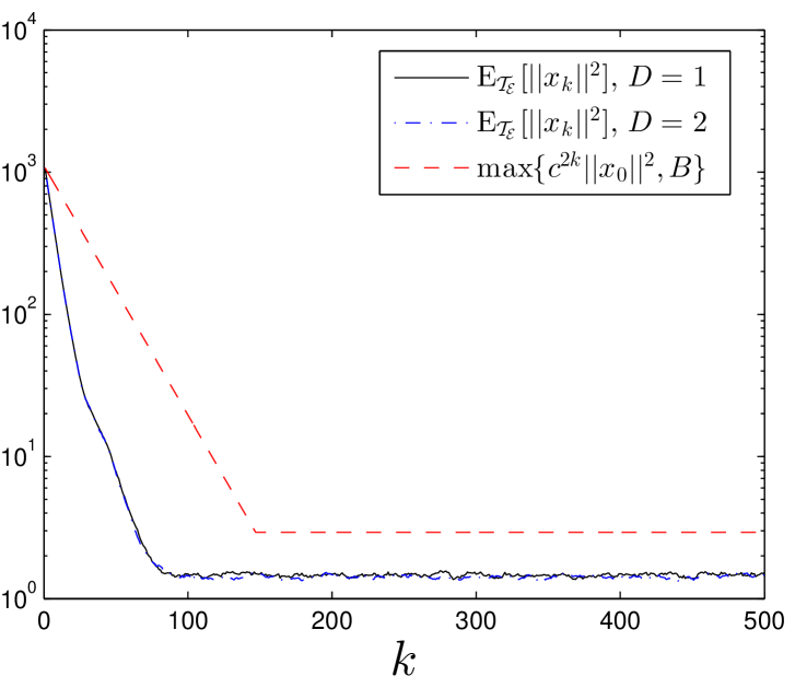
The process noise is drawn from a Gaussian distribution, with covariance $M$. To find the critical value $B^{*}=12.92$ in Proposition IV.6, we use the method described in the proof of Lemma IV.13 and the discussion subsequent to it. We performed simulations for $1000$ realizations of process noise and packet drops, all starting from the same initial condition. Then, for each time step $k$, we computed the empirical mean of the various quantities. This is illustrated in Figures 2 and 3. We performed simulations with $D=1$ and $D=3$, and in each case $D+\mathcal{B}=3$. Figure 2 shows that the control objective (7) is satisfied, as guaranteed by Theorem V.1. For $D=3$, one can see that the control objective is met more conservatively, which is consistent with the intuitive interpretation of the transmission policies given in Section III-B.

Figure 2: Plot of the evolution of the empirical mean $\mathbb{E}_{\mathcal{T}_{\mathcal{E}}}\left[x_{k}^{2}\right]$ for the scalar example under the event-triggered transmission policy (12) with $D=1$ and $D=3$ and the performance bound, $\max\{c^{2k}x_{0}^{2},B\}$.

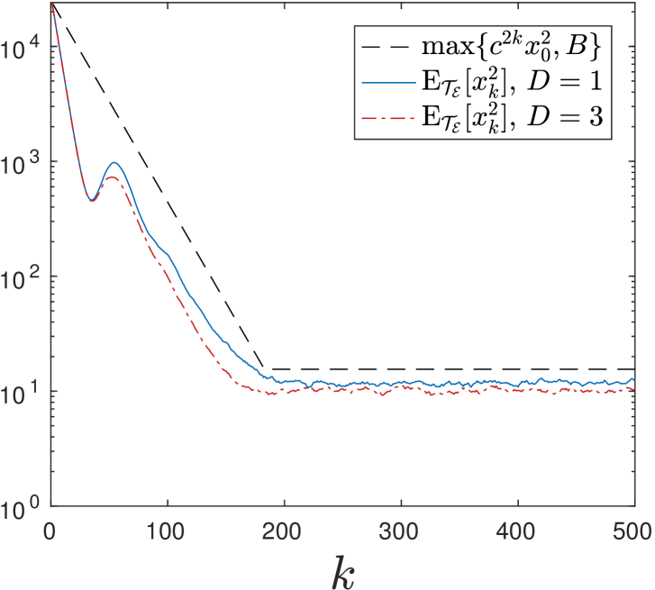
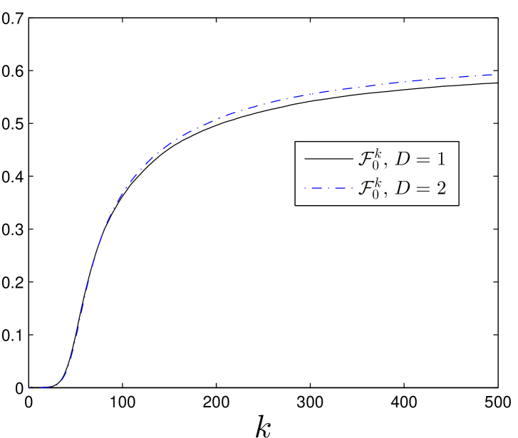
Figure 3 shows the empirical running transmission fractions for $D=1$ and $D=3$, as well as the upper bound on the transmission fraction $\mathcal{F}_{0}^{\infty}$ in the case of $D=1$ obtained in Proposition V.4. In the case of $D=3$, this quantity is $1$.

Figure 3: Plot of the evolution of the empirical running transmission fraction $\mathcal{F}_{0}^{k}$ for the scalar example under the event-triggered transmission policy (12) for $D=1$ and $D=3$, and the theoretical bound on the asymptotic transmission fraction $\mathcal{F}_{0}^{\infty}$ in the case of $D=1$ obtained in Proposition V.4. For $D=3$, the latter is $1$. For comparison, the plot also shows the empirical running transmission fractions in the case of $D=1$ and $p=1$ (perfect channel) and for a periodic policy with period $T=4$.

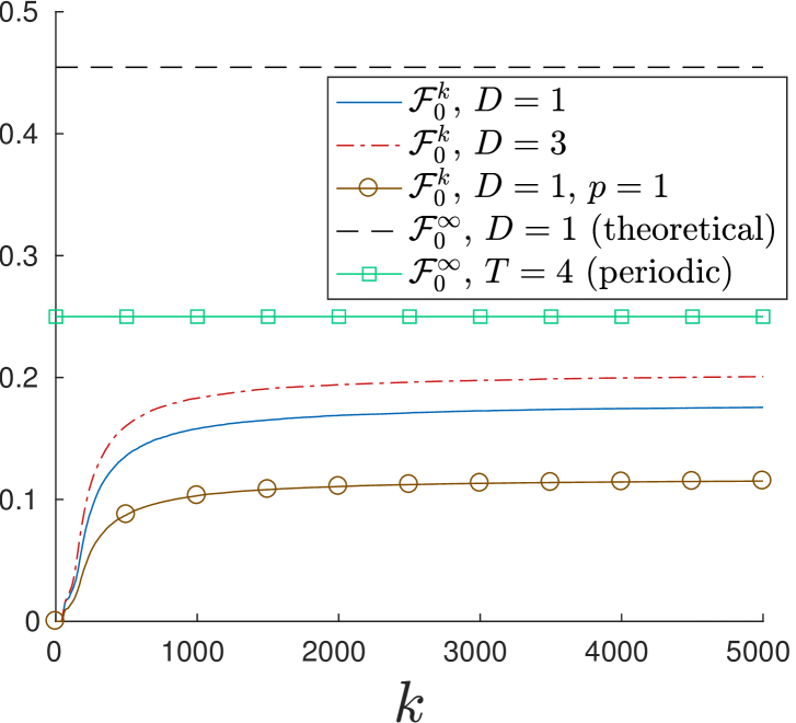
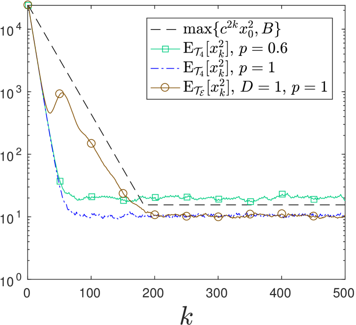
As expected, the conservativeness of the implementation with $D=3$ is reflected in a higher transmission fraction and in the conservativeness with which the control objective is satisfied. We found the optimal sufficient period for a periodic transmission policy, cf. Remark V.6, to be $1$. Thus, the transmission fraction for the optimal sufficient periodic transmission policy is $1$, which is higher than both the theoretical and the actual transmission fractions for our implementation with $D=1$. Figure 3 also shows the running transmission fraction in the case of $D=1$ and $p=1$ (perfect channel) and for a periodic policy with period $T=4$. We see that the proposed policy automatically adjusts its transmission fraction with changes in the dropout probability. Figure 4 shows the evolution of the performance function under the periodic policy with period $T=4$ in the case of a deterministic channel ($p=1$) and with a dropout probability of $(1-p)=0.4$. This is an example of a policy that works for a perfect channel ($p=1$) but does not work for an imperfect one ($p=0.6$). Although the transmission fraction for this policy is higher than that of our policy (cf. Figure 3), it still fails to meet the control objective in the case of $p=0.6$, demonstrating the usefulness of the proposed event-triggered policy over a periodic policy.

Figure 4: Plot of the evolution of the empirical mean $\mathbb{E}_{\mathcal{T}_{4}}\left[x_{k}^{2}\right]$ for the scalar example under the periodic transmission policy with period $T=4$ with $p=1$ (deterministic channel) and $p=0.6$ and the performance bound, $\max\{c^{2k}x_{0}^{2},B\}$. Also shown is the empirical mean $\mathbb{E}_{\mathcal{T}_{\mathcal{E}}}\left[x_{k}^{2}\right]$ under the event-triggered transmission policy (12) with $D=1$ and $p=1$.

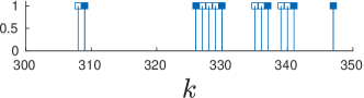
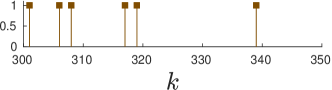
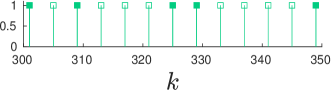
Finally, Figure 5 shows sample transmission and reception sequences for the event-triggered policy with $D=1$ and $p=0.6$ and $p=1$. We also show corresponding sequences for a periodic policy with period $T=4$ and $p=0.6$. The plots show an arbitrarily chosen interval of $50$ time steps for each transmission and reception to be clearly distinguished.

(a) Event-triggered, $D=1$, $p=0.6$

(b) Event-triggered, $D=1$, $p=1$

(c) Periodic, $T=1$, $p=0.6$

Figure 5: Sample transmission and reception sequences for the event-triggered transmission policy (12) with (a) $D=1$ under $p=0.6$ and (b) $D=1$ under $p=1$ and for (c) a periodic policy with period $T=4$ and under $p=0.6$. In each plot, an empty square corresponds to a “transmission, but no reception” and a filled square corresponds to a “transmission and successful reception”.

Vector system

We consider the dynamics (35) with the following system matrices

$$A=\begin{bmatrix}0.8&0.5\\ -0.5&1\end{bmatrix},\ Q=\begin{bmatrix}1&0\\ 0&1\end{bmatrix},$$

$$L=\begin{bmatrix}0.1310&-0.5000\\ 0.5000&-1.8820\end{bmatrix},\ \Sigma=\begin{bmatrix}0.1000&0.0500\\ 0.0500&0.1000\end{bmatrix},$$

and the parameters $p=0.8$ and $c=0.98$. For this system, we get $B^{*}=2.44$ and chose $B=2.93$. The initial condition is $x(0)=B.[10-5]^{T}$. We performed the same number of simulations as in the scalar example to compute the empirical mean of the various relevant quantities. The results of simulations under the event-triggered transmission policy (36) are illustrated in Figures 6 and 7. Figure 6 shows that the control objective is met, as stated in Theorem VI.2. The conservativeness that results from the use of the upper bounds from Proposition VI.1 in the definition of the event-trigger criterium is quite apparent from the gap between the control objective and the actual trajectories of $\mathbb{E}_{\bar{\mathcal{T}}_{\mathcal{E}}}\left[h_{k}\right]$ compared to Figure 2. Figure 7 also shows that, as in the scalar case, smaller $D$ results in a less conservative and more efficient design.

Figure 6: Plot of the evolution of the empirical mean $\mathbb{E}_{\mathcal{T}_{\mathcal{E}}}\left[\|x_{k}\|^{2}\right]$ for the vector example under the event-triggered transmission policy (36) with $D=1$ and $D=2$ and the performance bound, $\max\{c^{2k}\|x_{0}\|^{2},B\}$.

Figure 7: Plot of the evolution of the empirical running transmission fraction $\mathcal{F}_{0}^{k}$ for the vector example under the event-triggered transmission policy (36) for $D=1$ and $D=2$.

VIII Conclusions

We have designed an event-triggered transmission policy for scalar linear systems under packet drops. The control objective consists of achieving second-moment stability of the plant state with a given exponential rate of convergence to an ultimate bound in finite time. The synthesis of our policy is based on a two-step design procedure. First, we consider a nominal quasi-time-triggered policy where no transmission occurs for a given number of timesteps, and then transmissions occur on every time step thereafter. Second, we define the event-trigger policy by evaluating the expectation of the system performance at the next reception time given the current information under the nominal policy, and prescribe a transmission if this expectation does not meet the objective. We have also characterized the efficiency of our design by providing an upper bound on the fraction of the expected number of transmissions over the infinite time horizon. Finally, we have discussed the extension to the vector case, and highlighted the challenges in characterizing the efficiency of the event-triggered design. Future work will seek to address these challenges in the vector case, incorporate measurement noise, output measurements, lossy acknowledgments and will investigate the possibilities for optimizing the two-step design of event-triggered transmission policies, formally characterize the robustness advantages of event-triggered versus time-triggered control, and investigate the role of quantization and information-theoretic tools to address questions about necessary and sufficient data rates.

Appendix: Glossary of symbols

For the reader’s reference, we present here a list of the symbols most frequently used along the paper.

• State variables and functions

  • $x_{k}$: plant state at time $k$

  • $v_{k}$: process noise at time $k$

  • $\hat{x}_{k}$: sensor’s estimate of plant state at time $k$ given the ‘history’ up to time $k-1$

  • $\hat{x}_{k}^{+}$: controller’s estimate of plant state at time $k$ given ‘history’ up to time $k$, including any reception at time $k$

  • $e_{k}\triangleq x_{k}-\hat{x}_{k}$: sensor estimation error

  • $e_{k}^{+}\triangleq x_{k}-\hat{x}_{k}^{+}$: controller estimation error

  • $u_{k}\triangleq L\hat{x}_{k}^{+}$: control action at time $k$

  • $I_{k}$: information available to the sensor at time $k$ before the decision to transmit or not

  • $I_{k}^{+}$: information available to the controller at time $k$, which can also be computed by the sensor

  • $h_{k}$: value of performance function at time $k$

• System and performance parameters

  • $a$: open-loop ‘gain’

  • $\mkern 1.5mu\overline{\mkern-1.5muM\mkern-1.5mu}\mkern 1.5mu\triangleq\frac{M}{a^{2}-1}$: here $M$ is the covariance of $v_{k}$

  • $\bar{a}\triangleq a+L$: closed-loop ‘gain’ in the case of perfect transmissions on all time steps

  • $(1-p)$: probability of dropping a packet

  • $B$: ultimate bound for second moment of plant state

  • $c^{2}\in(0,1)$: prescribed convergence rate for second moment of plant state

• Transmission and reception process variables

  • $t_{k}\in\{0,1\}$: no transmission/transmission at time $k$

  • $r_{k}\in\{0,1\}$: no reception/reception at time $k$

  • $R_{k}$: latest reception time before $k$

  • $R_{k}^{+}$: latest reception time up to (including) $k$

  • $S_{j}$: $j^{\text{th}}$ reception time

• Symbols related to transmission policy

  • $\mathcal{T}_{k}^{D}$: nominal transmission policy at time $k$ with parameter $D$

  • $G_{k}^{D}$: look-ahead criterion at time $k$ with parameter $D$

  • $\mathcal{T}_{\mathcal{E}}$: proposed event-triggered transmission policy

  • $D$: ‘idle duration’ in the nominal policy and ‘look-ahead horizon’ in event-triggered policy

  • $T_{j}$: first time a transmission occurs after $S_{j}$ under $\mathcal{T}_{\mathcal{E}}$

  • $J_{k}^{D}$: performance-evaluation function at time $k$ with parameter $D$

  • $H$: open-loop performance evolution function

  • $g_{D}(b)\triangleq\frac{b^{D}}{1-b(1-p)}$

Pavankumar Tallapragada received the B.E. degree in Instrumentation Engineering from SGGS Institute of Engineering $\&$ Technology, Nanded, India in 2005, M.Sc. (Engg.) degree in Instrumentation from the Indian Institute of Science, Bangalore, India in 2007 and the Ph.D. degree in Mechanical Engineering from the University of Maryland, College Park in 2013. He held a postdoctoral position at the University of California, San Diego during 2014 to 2017. He is currently an Assistant Professor in the Department of Electrical Engineering at the Indian Institute of Science, Bengaluru, India. His research interests include event-triggered control, networked control systems, distributed control and networked transportation systems.

Massimo Franceschetti (M’98-SM’11) received the Laurea degree (with highest honors) in computer engineering from the University of Naples, Naples, Italy, in 1997, the M.S. and Ph.D. degrees in electrical engineering from the California Institute of Technology, Pasadena, CA, in 1999, and 2003, respectively. He is Professor of Electrical and Computer Engineering at the University of California at San Diego (UCSD). Before joining UCSD, he was a postdoctoral scholar at the University of California at Berkeley for two years. He has held visiting positions at the Vrije Universiteit Amsterdam, the École Polytechnique Fédérale de Lausanne, and the University of Trento. His research interests are in physical and information-based foundations of communication and control systems. He is co-author of the book “Random Networks for Communication” published by Cambridge University Press. Dr. Franceschetti served as Associate Editor for Communication Networks of the IEEE Transactions on Information Theory (2009 – 2012), as associate editor of the IEEE Transactions on Control of Network Systems (2013-16) and as Guest Associate Editor of the IEEE Journal on Selected Areas in Communications (2008, 2009). He is currently serving as Associate Editor of the IEEE Transactions on Network Science and Engineering. He was awarded the C. H. Wilts Prize in 2003 for best doctoral thesis in electrical engineering at Caltech; the S.A. Schelkunoff Award in 2005 for best paper in the IEEE Transactions on Antennas and Propagation, a National Science Foundation (NSF) CAREER award in 2006, an Office of Naval Research (ONR) Young Investigator Award in 2007, the IEEE Communications Society Best Tutorial Paper Award in 2010, and the IEEE Control theory society Ruberti young researcher award in 2012.

Jorge Cortés (M’02-SM’06-F’14) received the Licenciatura degree in mathematics from Universidad de Zaragoza, Zaragoza, Spain, in 1997, and the Ph.D. degree in engineering mathematics from Universidad Carlos III de Madrid, Madrid, Spain, in 2001. He held postdoctoral positions with the University of Twente, Twente, The Netherlands, and the University of Illinois at Urbana-Champaign, Urbana, IL, USA. He was an Assistant Professor with the Department of Applied Mathematics and Statistics, University of California, Santa Cruz, CA, USA, from 2004 to 2007. He is currently a Professor in the Department of Mechanical and Aerospace Engineering, University of California, San Diego, CA, USA. He is the author of Geometric, Control and Numerical Aspects of Nonholonomic Systems (Springer-Verlag, 2002) and co-author (together with F. Bullo and S. Martínez) of Distributed Control of Robotic Networks (Princeton University Press, 2009). He has been an IEEE Control Systems Society Distinguished Lecturer (2010-2014) and is an elected member for 2018-2020 of the Board of Governors of the IEEE Control Systems Society. His current research interests include distributed control and optimization, network science, opportunistic state-triggered control and coordination, reasoning under uncertainty, and distributed decision making in power networks, robotics, and transportation.

References

- [1] P. Tallapragada, M. Franceschetti, and J. Cortés, “Event-triggered stabilization of scalar linear systems under packet drops,” in Allerton Conf. on Communications, Control and Computing, Monticello, IL, Sep. 2016, pp. 1173–1180.
- [2] K. D. Kim and P. R. Kumar, “Cyber-physical systems: A perspective at the centennial,” Proceedings of the IEEE, vol. 100, no. Special Centennial Issue, pp. 1287–1308, 2012.
- [3] J. Sztipanovits, X. Koutsoukos, G. Karsai, N. Kottenstette, P. Antsaklis, V. Gupta, B. Goodwine, J. Baras, and S. Wang, “Toward a science of cyber-physical system integration,” Proceedings of the IEEE, vol. 100, no. 1, pp. 29–44, 2012.
- [4] S. Tatikonda and S. Mitter, “Control under communication constraints,” IEEE Transactions on Automatic Control, vol. 49, no. 7, pp. 1056–1068, 2004.
- [5] G. N. Nair, F. Fagnani, S. Zampieri, and R. J. Evans, “Feedback control under data rate constraints: an overview,” Proceedings of the IEEE, vol. 95, no. 1, pp. 108–137, 2007.
- [6] S. Yüksel and T. Başar, Stochastic Networked Control Systems: Stabilization and Optimization under Information Constraints, ser. Systems & Control: Foundations & Applications. Boston, MA: Birkhäuser, 2013.
- [7] L. Schenato, B. Sinopoli, M. Franceschetti, K. Poolla, and S. S. Sastry, “Foundations of control and estimation over lossy networks,” Proceedings of the IEEE, vol. 95, no. 1, pp. 163–187, 2007.
- [8] V. Gupta and N. C. Martins, “On stability in the presence of analog erasure channels between controller and actuator,” IEEE Transactions on Automatic Control, vol. 55, no. 1, pp. 175–179, 2010.
- [9] V. Gupta, “Estimation and control over networks,” in Encyclopedia of Systems and Control, J. Baillieul and T. Samad, Eds. New York: Springer, 2015.
- [10] P. Tabuada, “Event-triggered real-time scheduling of stabilizing control tasks,” IEEE Transactions on Automatic Control, vol. 52, no. 9, pp. 1680–1685, 2007.
- [11] X. Wang and M. D. Lemmon, “Event-triggering in distributed networked control systems,” IEEE Transactions on Automatic Control, vol. 56, no. 3, pp. 586–601, 2011.
- [12] W. P. M. H. Heemels, K. H. Johansson, and P. Tabuada, “An introduction to event-triggered and self-triggered control,” in IEEE Conf. on Decision and Control, Maui, HI, 2012, pp. 3270–3285.
- [13] D. Lehmann and J. Lunze, “Event-based control using quantized state information,” in IFAC Workshop on Distributed Estimation and Control in Networked Systems, Annecy, France, Sep. 2010, pp. 1–6.
- [14] L. Li, X. Wang, and M. D. Lemmon, “Stabilizing bit-rate of disturbed event triggered control systems,” in Proceedings of the 4th IFAC Conference on Analysis and Design of Hybrid Systems, Eindhoven, Netherlands, Jun. 2012, pp. 70–75.
- [15] Y. Sun and X. Wang, “Stabilizing bit-rates in networked control systems with decentralized event-triggered communication,” Discrete Event Dynamic Systems, vol. 24, no. 2, pp. 219–245, 2014.
- [16] E. Garcia and P. J. Antsaklis, “Model-based event-triggered control for systems with quantization and time-varying network delays,” IEEE Transactions on Automatic Control, vol. 58, no. 2, pp. 422–434, 2013.
- [17] J. Pearson, J. P. Hespanha, and D. Liberzon, “Control with minimum communication cost per symbol,” in IEEE Conf. on Decision and Control, Los Angeles, CA, 2014, pp. 6050–6055.
- [18] P. Tallapragada and J. Cortés, “Event-triggered stabilization of linear systems under bounded bit rates,” IEEE Transactions on Automatic Control, vol. 61, no. 6, pp. 1575–1589, 2016.
- [19] P. Tallapragada, M. Franceschetti, and J. Cortés, “Event-triggered control under time-varying rate and channel blackouts,” Automatica, 2015, submitted.
- [20] K. J. Åström and B. M. Bernhardsson., “Comparison of Riemann and Lebesgue sampling for first-order stochastic systems,” in IEEE Conf. on Decision and Control, Las Vegas, NV, Dec. 2002, pp. 2011–2016.
- [21] T. Henningsson, E. Johannesson, and A. Cervin, “Sporadic event-based control of first-order linear stochastic systems,” Automatica, vol. 44, no. 11, pp. 2890–2895, 2008.
- [22] X. Meng and T. Chen, “Optimal sampling and performance comparison of periodic and event based impulse control,” IEEE Transactions on Automatic Control, vol. 57, no. 12, pp. 3252–3259, 2012.
- [23] B. Demirel, V. Gupta, D. E. Quevedo, and M. Johansson, “On the trade-off between control performance and communication cost in event-triggered control,” arXiv preprint arXiv:1501.00892, 2015.
- [24] M. Rabi and K. H. Johansson, “Scheduling packets for event-triggered control,” in European Control Conference, Budapest, Hungary, Aug. 2009.
- [25] R. Blind and F. Allgöwer, “The performance of event-based control for scalar systems with packet losses,” in IEEE Conf. on Decision and Control, Maui, HI, Dec. 2012, pp. 6572–6576.
- [26] M. H. Mamduhi, D. Tolić, A. Molin, and S. Hirche, “Event-triggered scheduling for stochastic multi-loop networked control systems with packet dropouts,” in IEEE Conf. on Decision and Control, Los Angeles, CA, Dec. 2014, pp. 2776–2782.
- [27] A. Molin and S. Hirche, “On the optimality of certainty equivalence for event-triggered control systems,” IEEE Transactions on Automatic Control, vol. 58, no. 2, pp. 470–474, 2013.
- [28] O. C. Imer and T. Basar, “Optimal control with limited controls,” in American Control Conference, Minneapolis, MN, Jun. 2006, pp. 298–303.
- [29] R. P. Anderson, D. Milutinović, and D. V. Dimarogonas, “Self-triggered sampling for second-moment stability of state-feedback controlled SDE systems,” Automatica, vol. 54, pp. 8–15, 2015.
- [30] D. E. Quevedo, V. Gupta, W. Ma, and S. Yüksel, “Stochastic stability of event-triggered anytime control,” IEEE Transactions on Automatic Control, vol. 59, no. 12, pp. 3373–3379, 2014.
- [31] P. Minero, M. Franceschetti, S. Dey, and G. N. Nair, “Data rate theorem for stabilization over time-varying feedback channels,” IEEE Transactions on Automatic Control, vol. 54, no. 2, pp. 243–255, 2009.
- [32] M. Franceschetti and P. Minero, “Elements of information theory for networked control systems,” in Information and Control in Networks, G. Como, B. Bernhardsson, and A. Rantzer, Eds. New York: Springer, 2014, vol. 450, pp. 3–37.