An Empirical Study of Cycle Toggling Based Laplacian Solvers

Abstract

We study the performance of linear solvers for graph Laplacians based on the combinatorial cycle adjustment methodology proposed by [Kelner-Orecchia-Sidford-Zhu STOC-13]. The approach finds a dual flow solution to this linear system through a sequence of flow adjustments along cycles. We study both data structure oriented and recursive methods for handling these adjustments.

The primary difficulty faced by this approach, updating and querying long cycles, motivated us to study an important special case: instances where all cycles are formed by fundamental cycles on a length $n$ path. Our methods demonstrate significant speedups over previous implementations, and are competitive with standard numerical routines.

Figure 1: Performance profile of cycle-toggle time. The relative performance ratio of a method is its cycle-toggle time $/$ best cycle toggle time for a single problem. This plot shows the fraction of problems that are within a distance from this relative performance ratio. The faster a method converges to 1 on this plot, the better its performance relative to the others.

1 Introduction

Much progress has been made recently toward the development of graph Laplacian linear solvers that run in linear times polylogarithmic time [16, 17, 18, 21, 24, 9, 15]. These methods use a combination of combinatorial, randomized, and numerical methods to obtain algorithms that provably solve any graph Laplacian linear system in time faster than sorting to constant precision.

Linear solvers for graph Laplacians have a wide range of applications. They can be used to solve problems such as image denoising, finding maximum flows in a graph, and more generally solving linear programs with an underlying graph, such as, minimum cost maximum flow and graph theoretic regression problems  [5, 30, 8, 11, 20, 23, 22, 7, 19]. Many of these applications stem from the following connection through optimization: solving linear systems is equivalent to minimizing $\ell_{2}$ norms over a suitable set. Many applications can in turn be viewed as solving a problem based on a different norm, such as $\ell_{1}$ or $\ell_{\infty}$. The gap between these norms can be addressed through iterative schemes, leading to algorithms that repeatedly call linear system solvers.

Laplacian linear solvers can be divided into primal solvers, which solve for a set of vertex potentials, and dual solvers, which solve for a set of edge flows that minimize energy. The theoretically fastest known solvers are primal solvers which use recursive preconditioned Chebyshev iterations [9]. On the other hand, the near-linear time algorithm with the simplest description works in the dual space [18]. We believe that the fastest solver will be one that combines both a potential and flow based approach. The goal of this paper is to empirically better understand flow based methods in order to facilitate their integration into primal-dual algorithmic schemes.

Our main contribution is an experimental investigation of different cycle-toggling implementations and an examination of the resulting performance implications. To that end we introduce a class of synthetic, weighted graphs that are both simple enough to reason about theoretically, and rich enough to yield interesting behavior for cycle-toggling implementations. One of the implementations we use is a novel divide-and-conquer technique which we describe. We end with a comparison of cycle-toggling implementations to conjugate gradient.

2 Background

2.1 Definitions

Symmetric diagonally dominant (SDD) matrices and M matrices can be reduced to Laplacian matrices asymptotically quickly, so the fastest SDD solvers rely on Laplacian solvers. Laplacians are equivalent to graphs, which we define as $G=(V,E,\boldsymbol{\mathit{w}})$ where $V$ is a vertex set, $E$ a set of edges, and $\boldsymbol{\mathit{w}}$ a set of edge weights. The Laplacian is given by

$$\boldsymbol{\mathit{L}}_{i,j}=\begin{cases}\deg(i)&\text{if }i=j\\ -\boldsymbol{\mathit{w}}_{ij}&\text{otherwise}\end{cases},$$

where $\deg(i)$ is the weighted degree, or sum of incident edge weights on vertex $i$. The problem of interest is to solve $L\boldsymbol{\mathit{x}}=\boldsymbol{\mathit{b}}$ for $\boldsymbol{\mathit{x}}$ given $\boldsymbol{\mathit{b}}$.

There is a useful electrical network interpretation of

$$\boldsymbol{\mathit{x}}^{T}\boldsymbol{\mathit{L}}\boldsymbol{\mathit{x}}=\sum_{uv\in E}\boldsymbol{\mathit{w}}_{uv}\left(\boldsymbol{\mathit{x}}_{u}-\boldsymbol{\mathit{x}}_{v}\right)^{2}$$

where $\boldsymbol{\mathit{x}}_{u}-\boldsymbol{\mathit{x}}_{v}$ can be viewed as voltages [13], and $\boldsymbol{\mathit{w}}_{uv}$ represents the inverse of resistance in terms of energy dissipation. This definition of resistances gives a corresponding electrical flow interpretation, which forms the basis of the Kelner et al.s algorithm [18], which we will call KOSZ. In this flow interpretation the problem translates to finding a flow $\boldsymbol{\mathit{f}}$ that meets demands given by $\boldsymbol{\mathit{b}}$, and minimizes $\sum_{e}\boldsymbol{\mathit{r}}_{e}\boldsymbol{\mathit{f}}_{e}^{2}$.

2.2 Existing Methods

The underlying algebraic operations of theoretically fast graph Laplacian solvers can be viewed as either directly manipulating the potential vectors, or the dual flows. To date, empirical studies of these solvers have focused on the dual flow based algorithms, leading to mixed results [3, 14, 4], most of which are not directly competitive with numerical methods such as conjugate gradient (CG) [26] or multigrid [6], and instead bound iteration count. In this paper, we study these dual algorithms with additional insights obtained during the study of vector based primal algorithms. We show that the dual adjustment stages can be unraveled in ways similar to recursive steps in vector solvers. This allows us to both improve the dual adjustment routine, as well as having it interact with classical iterative methods such as conjugate gradient. Our main experimental results are on improving the performance of both data structural and recursive approaches, and comparing their performance to conjugate gradient.

Crucial to the performance of these dual flow solvers is the cycle adjustment process: here most of the cycles are long, thus cost-prohibitive to adjust in nearly-linear time. To obtain nearly-linear performance, these updates are restricted to fundamental cycles of a tree. This restriction allows updates to be processed using tree data structures. These structures are based on “virtual tree” representations of trees that allow each path to be broken down into $O(\log{n})$ subtrees. Updating cycles is then done by accessing and modifying the corresponding labels. Handling these updates efficiently has proven to be directly related to the performance of implementations of this algorithm [18].

2.3 KOSZ overview

The KOSZ algorithm [18] randomly selects cycles and adjusts the flow along a cycle to bring it to the minimum energy state, while maintaining a feasible flow. These cycles are formed by first picking a spanning tree $T$. Then each off-tree edge forms a cycle, known as a fundamental cycle with respect to $T$. Collectively these cycles form a fundamental cycle basis which spans the cycle space of the graph.

Given a cycle of length $k$ with flows $\boldsymbol{\mathit{f}}_{1}\ldots\boldsymbol{\mathit{f}}_{k}$ oriented in the forward direction, our goal is to find a change in flow $\Delta$ that minimizes the updated flow energy

$$\sum_{i}\boldsymbol{\mathit{r}}_{i}\left(\boldsymbol{\mathit{f}}_{i}+\Delta\right)^{2}\\ =\left(\sum_{i}\boldsymbol{\mathit{r}}_{i}\right)\Delta^{2}+2\left(\sum_{i}\boldsymbol{\mathit{r}}_{i}\boldsymbol{\mathit{f}}_{i}\right)\Delta_{i}+\sum_{i}\boldsymbol{\mathit{r}}_{i}\boldsymbol{\mathit{f}}_{i}^{2}.$$

This is minimized by setting

$$\Delta=-\frac{\sum_{i}\boldsymbol{\mathit{r}}_{i}\boldsymbol{\mathit{f}}_{i}}{\sum_{i}\boldsymbol{\mathit{r}}_{i}}.$$

The choice of cycles to update is dictated by the stretch of the off-tree edges. Conceptually, the stretch of an edge is the length of the detour that must be traversed in the tree if the edge is removed. This removal “stretches” the edge across the new path. Here length is measured in terms of resistances, or inverse edge weight $\frac{1}{\boldsymbol{\mathit{w}}_{e}}$. For an edge $e$, let the (unique) simple path between its end points in tree be $P_{T}(e)$, then

$$str(e)=\boldsymbol{\mathit{w}}_{e}\sum_{e^{\prime}\in P_{T}(e)}\frac{1}{\boldsymbol{\mathit{w}}_{e^{\prime}}}.$$

The main result of [18] is:

Theorem 2.1.

Given a tree with total stretch $S$, repeatedly sampling the edges randomly with probability proportional to $1+str(e)$ and bringing the corresponding cycle to its minimum energy state gives an $1+\epsilon$-approximate answer in $O((m+S)\log(1/\epsilon))$ iterations.

3 Implementing Cycle Toggling

Cycle-toggling methods require many cycle updates for energy minimization, necessitating quick update operations. We need to support the following operations on a tree $T$, where each edge $e$ is associated with a fixed resistance $\boldsymbol{\mathit{r}}_{e}$ and a flow $\boldsymbol{\mathit{f}}_{e}$:

1. Query: Compute sums of $\boldsymbol{\mathit{r}}_{e}$ and $\boldsymbol{\mathit{r}}_{e}\boldsymbol{\mathit{f}}_{e}$ along a path in $T$.

2. Update: Increment all the flows on a path in $T$ by $\Delta$.

Although these updates are not adaptive, the result of each update does depend on all previous updates that interact with the path. This creates fundamental restrictions on cycle-toggling speed. This is especially true when considering any possible parallelism of updating multiple cycles simultaneously.

In the rest of this section we consider two different schemes for achieving fast cycle updates. The first uses data structures similar to the ones used by the KOSZ algorithm to update each cycles in $O(\log(n))$ time. The second is a divide-and-conquer approach we introduce, which contracts the path based on preselected cycle updates.

3.1 Reduction to Balanced BSTs

We hope to provide the reader with a brief overview of our data structure approach along with the approach used by KOSZ [18]. The KOSZ data structures are based on top-down partitions of trees. Our implementations are based on a variant of this that uses binary search trees as building blocks. To help explain this, we first consider the easier case in which $T$ is just a path, where we can solve the problem by building a static balanced binary search tree (BST) [10]. Any subtree in the BST corresponds to an interval in the path, which can be decomposed into a disjoint union of at most $2\log n$ subtrees and nodes in the BST. To support our query and update operations, we add two pieces of information at every node $v$:

1. The sum, $\sum_{i}r_{i}f_{i}$ where $i\in$ the subtree containing $v$

2. A lazy tag $t$, denoting the pending changes of flow in this subtree, caused by updates to parents.

The BST can answer the interval queries by adding up the sum fields of the corresponding subtrees. Note that this requires the lazy tag fields of all ancestors of the nodes added to be $0$. This can be handled by ‘pushing down’ such fields as we access the BST. The updates involve modifying the lazy tag and sum fields of the subtrees correspondingly. This gives us a $O(\log n)$ per operation algorithm for the case where $T$ is a path.

(a) Heavy path re-rooted at separator vertex

(b) Virtual tree where heavy path is represented by the BST that stores it

Figure 2: One step of a heavy-light decomposition. Triangles are subtrees labeled with size.

A classic way to generalize the path case to a tree is to use a heavy-light decomposition (HLD) [27]. Here, one first arbitrarily roots the tree. Then for every vertex $u$, we denote $v$ as the child of $u$ whose subtree has the largest size (i.e. contains most vertices). We mark every edge $(u,v)$ as heavy and say that all edges not marked heavy are light. An unextendable path of heavy edges is called a heavy chain. This decomposes the tree into heavy chains and light edges.

The key fact about this decomposition is that for any vertex $v$, its path to the root intersects at most $O(\log n)$ heavy chains and $O(\log n)$ light edges. Therefore, to support query and update operations on a tree, it suffices to handle the light edges and support these operations on heavy paths. For the latter, this is exactly the special path case and we can use BSTs described above. This leads to a theoretical time bound $O(\log^{2}n)$ per operation, but a quite good running time experimentally.

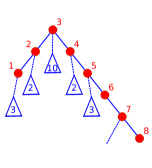
This method is connected to the data structures used in KOSZ via virtual trees. Such a tree contains all the BST edges for heavy chains along with light edges. An example of creating a virtual tree from a HLD is shown in Figure 2. We can further optimize cycle updates by reducing the virtual tree height. A path between $u$ and $v$ in the original tree can be decomposed into the disjoint union of left-subtrees of nodes in the path between $u$ and $v$ in the virtual tree. In HLD, this virtual tree has height $O(\log^{2}n)$ (since each BST has height $O(\log n)$ and there are at most $O(\log n)$ heavy chains encountered in any path), so the time bound is $O(\log^{2}n)$.

A better virtual tree can be constructed in a recursive manner. Consider the heavy chain starting from the root of $T$. Using the properties of heavy chains, one can prove that there exists a node $v$ in the heavy chain, whose removal splits $T$ into subtrees which have size at most half of the original tree size. We use $v$ as the root of the BST for this heavy chain, and construct recursively. The virtual tree satisfies the property that any child has at most half the size of its parent, so it has height at most $\log n$. This gives us a $O(\log n)$ per operation algorithm. Compared to the recursive-separator based routine from [18], this scheme fixes the heavy path in addition to the root of the virtual tree. While this only changes the constants in the analysis, in terms of implementation it allows us to directly use the binary tree routine for paths mentioned above.

3.2 Recursive Divide-and-Conquer

The other main approach that we explore is a recursive divide-and-conquer scheme. The KOSZ solver treats cycle updates as an online process, a cycle is sampled, then updated, before another cycle is sampled. We consider the potential of an offline approach where we preselect $N$ cycles, and use knowledge of this set to speed up the update of the set as a whole. This method recursively divides the $N$ cycles in half until the subsets are each of size less than $n$. The cycles in the last level of the recursion are then updated in their preselected order.

(a) Original Graph

(b) Subgraph 1,4

(c) Subgraph 2,3,5

(d) Contraction of(b)

(e) Contraction of(c)

Figure 3: Illustration of graph reduction and contraction in divide-and-conquer. 5 cycles are preselected in the original graph(a) and divided into two groups, cycles (1,4) and (2,3,5). These cycles induce subgraphs (b,c) which only include edges and vertices of the relevant cycles. These subgraphs are then path contracted (d,e) to further reduce size.

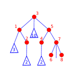
The speedup of this approach lies in the fact that we can reduce the problem to only the part of the graph involved in our preselected updates. We can further reduce the size of the graph by path contraction, condensing two edges if they are only updated when the other is updated. An example of this reduction and contraction is shown in Figure 3. This process results in several smaller graphs, where the cycles are updated, before pushing the cycle update information back up the recursive subgraph hierarchy. As this process resembles the recursive subgraph hierarchy of multigrid methods, we borrow the terms restriction and prolongation to describe the transfer of flow information up and down the hierarchy. This process is more formally captured in the following lemma.

Lemma 3.1.

Given a tree on $n$ vertices, and $N$ cycle updates, we can form a tree on $3N$ vertices, perform the corresponding cycle updates on them, and transfer the state back to the original graph. Furthermore, both the reduction and prolongation steps take $O(n)$ time.

This procedure is identical to the greedy elimination, or partial Cholesky factorization steps from the ultra-sparsification routines [29]. Recursively dividing the cycle set yields a recurrence of the form:

$$\mathcal{T}(N)=O(N)+2\mathcal{T}(N/2),$$

which solves to $\mathcal{T}(N)=O(N\log{N})$. If we set the size of our preselected cycle set to $O(n)$, then updating the entire set takes $O(n\log{n})$ work, leading to a cost of $O(\log{n})$ per update.

Unfortunately, the divide-and-conquer scheme does not parallelize naturally: the second recursive call still depends on the outcome of the first one. Furthermore, the bottleneck of this routine’s performance is the restriction and prolongation steps, which unlike multigrid can not be reused when we resample another set. A large part of the expense is that vertices and edges must be relabeled as the graph is reduced. Doing this in random order leads to random access of vertex and edge labels. We try to optimize this by either compressing the memory of the graph storage, or by reordering the updates within each batch. In the case that the tree is just a path, much of the vertex and edge labeling can be done implicitly, reducing the overhead.

4 Heavy Path Graphs

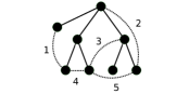
Here we introduce a class of model problems that we will use to test and analyze different cycle-toggling approaches. These graphs are constructed by adding edges between vertices on a path graph. Edge resistances are selected so that the low-stretch spanning tree of the resulting graph is always the underlying path. As a consequence the edges on the path have larger edge weights than the off-path edges, so we refer to this class of graphs as heavy path graphs. An example of such a graph is shown in Figure 4.

Figure 4: An example of a heavy path graph. The solid path edges are the low-stretch spanning tree of the graph.

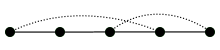
Our interest in these problems does not come from any real world application. Instead we believe these are natural models to consider when studying KOSZ and other cycle-toggling algorithms. We believe that this model can be tuned to have various stretch properties along with spectral and graph separator properties, though we do not explore that in this paper. Furthermore they allow us to explore very fundamental questions about data structures and cycle-toggling implementations.

This model simplifies many of the implementation issues associated with dynamic trees, as the paths are easier to handle than more general tree layouts. Specifically, we can use a static, perfectly balanced binary tree for the path. This likely has the least data structure overhead as the optimum separator of an interval is implicitly the middle. Furthermore, this allows us to store the tree in heap order, which means the tree paths can be mapped to a subinterval using bit operations, and the downward/upward propagations can be performed iteratively.

4.1 Example Models

There are many possible subclasses that belong to the heavy path graph model. We introduce several subclasses here for experimentation.

1. Fixed Cycle Length-1k: These graphs are composed of a tree path with random resistances between 1 and 10,000, combined with off-tree edges between every pair $(i,i+1000)$, e.g. an edge between vertices 1 and 1000, between vertices 2 and 1001, and so on.

2. Fixed Cycle Length-2: These graphs are composed of a tree path with random resistances between 1 and 10,000, combined with off-tree edges between every pair $(i,i+2)$, e.g. an edge between vertices 1 and 3, between vertices 2 and 4, and so on.

3. Random Cycle Length: These graphs are composed of a tree path with random resistances between 1 and 1000, combined with $n$ randomly selected off-tree edges, where $n$ is the number of vertices.

4. 2D Mesh: These graphs embed a tree path in a 2D mesh. The tree path resistances are chosen randomly between 1 and 1000.

5. 3D Mesh, Uniform Stretch: These graphs are similar to (4) but with a 3D mesh.

We then consider two different ways of setting resistances on the off-tree edges on all of the models above.

1. Uniform Stretch Resistances of off-tree edges are chosen so that stretch is 1 for every cycle.

2. Exponential Stretch Resistances of off-tree edges are chosen so that cycles have stretch sampled from an exponential distribution.

5 Experiments

5.1 Experimental Design

We now describe empirical evaluations of the cycle-toggling implementations from Section 3 on the class of graphs described in Section 4. As we only experiment on these path models, we can use cycle-toggling methods that will only work on a path, but we also employ their more general versions that will work on any graph. The four cycle-toggling implementations are as follows:

1. BST-based data structure for general graphs

2. Path-only BST decomposition

3. Recursive divide-and-conquer for general graphs

4. Path-only recursive divide-and-conquer

Additionally we implement a preconditioned conjugate gradient with diagonal scaling to compare against the cycle-toggling methods. We implemented all of these in C++ and also have a Python/Cython implementation of the general recursive method. All algorithm implementations, graph generators, and test results for this paper can be found at https://github.com/sxu/cycleToggling. We also experimented with Hoske et al.’s [14] implementation of cycle-toggling.

We use all of the generators described in Section 4.1 to create different heavy path graphs with a varying total stretch. We use vertex sizes of $5\times 10^{4}$, $10^{5}$, $5\times 10^{5}$, and $10^{6}$. For the fixed cycle length generators, we set $hop=1000$, and for the random cycle length generators, we set the number of off-tree edges to $2n$. To get an idea for the various stretch properties of these graphs, we list the total stretch for size $10^{6}$ in Table 1.

	Uniform	Exponential
Fixed Length-1k	1.01e6	1.12e6
Fixed Length-2	2.00e6	1.04e7
Random Length	2.00e6	1.30e7
2D Mesh	2.00e6	1.08e7
3D Mesh	3.82e6	2.27e7

Table 1: Total stretch for all graph models of size $10^{6}$. For each of the model problems in 4.1, this table shows the total stretch of cycles formed by adding edges to the underlying path. The models were generated with weights to create cycles with uniform stretch (all cycles with stretch 1), and exponential stretch(cycles with stretch chosen from an exponential distribution).

We also generate right hand side vectors $\boldsymbol{\mathit{b}}$ in two different ways to obtain both local and global behaviors.

1. Random: Randomly select $\boldsymbol{\mathit{x}}$ and form $\boldsymbol{\mathit{b}}=\boldsymbol{\mathit{L}}\boldsymbol{\mathit{x}}$,

2. (-1,1): Pick $\boldsymbol{\mathit{b}}$ to route $1$ unit of electrical flow from the left endpoint of the path to the right endpoint.

Experiments were performed on Mirasol, a shared memory machine at Georgia Tech, with 80 Intel(R) Xeon(R) E7-8870 processors at 2.40GHz. Problems were solved to a residual tolerance of $10^{-5}$.

5.2 Experimental Results

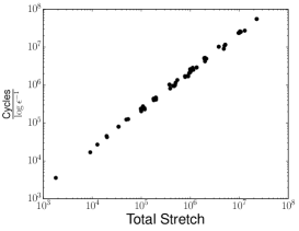
We first examine the asymptotic behavior of the cycle-toggling methods on all the test graphs. Figure 5 shows the number of cycles required for convergence as a function of total stretch. This figure only involves solves using the 0-1 right hand side as this was always a more difficult case.

Figure 5: KOSZ asymptotic dependence on tree stretch. The number of toggles required by KOSZ is shown as a function of tree stretch. The reasonable slope indicates a lack of large hidden constants in KOSZ complexity.

We omit results from the Hoske et al. implementation because we found its performance to be slower by a factor of $50$ than our cycle-toggling implementations. Their initialization costs are much higher than solve costs, making it prohibitively expensive to run on all of the test graphs in our set.

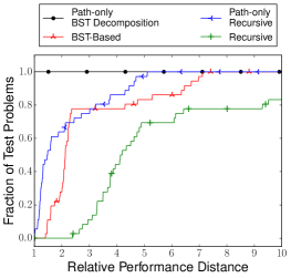
To visualize the comparison of cycle-toggling implementations on all the different test graphs, we utilize a performance profile plot shown in Figure 1. A performance profile [12] calculates, for some performance metric, the relative performance ratio between each solver and the best solver on every problem instance. In our case the metric of interest is the average cycle-toggle time, so for each method and every graph, the relative performance ratio is the method’s average cycle-toggle time divided by the lowest average cycle-toggle time over all methods. Then to capture how a method fares across the entire problem set, the performance profile shows the fraction of test problems (on the y-axis) that are within a distance (on the x-axis) from the relative performance ratio. This plot contains all the different model problems at every problem size tested.

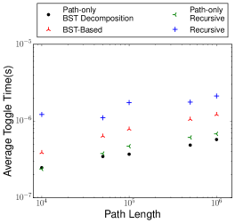
Weak scaling experiments, measuring cycle-toggle performance as graph size increases, are useful for predicting performance on larger problems. The scaling behavior was relatively similar across the model problems so we only show one example in Figure 6 for the 3D Unweighted Mesh with exponential stretch.

Figure 6: Weak scaling of cycle-toggle performance of all methods on unweighted 3D mesh model problems with exponential stretch. Average cycle-toggle time is shown as a function of problem size where an upward slope indicates decreased performance with larger problem size.

We examine how much time the recursive method spends restricting and prolonging flow in the recursive hierarchy, and how much time is spent doing cycle-toggles in Figure 7. Results are shown for the FixedLength-1k model with a slightly wider range of problem size than the other experiments. The solve time in this plot includes the sum of the other operation timings, along with memory allocation. We did this profiling with our Python/Cython implementation, but we believe the C++ performance is comparable.

Figure 7: Weak scaling of cycle-toggle performance for the recursive solver on FixedLength-1k model problems. Average cycle-toggle time is shown along with its most expensive sub-components: restriction, solve, and prolongation. Upward slopes indicate decreasing performance with problem size.

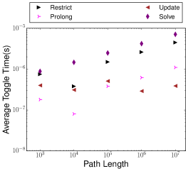
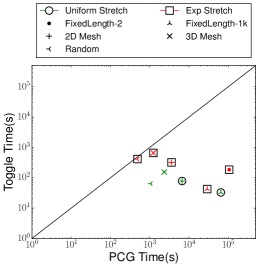
Figure 8 shows BST-based cycle-toggle timing results relative to PCG results. Points below the line indicate cycle-toggling was faster, while points above the line are slower. This plot only includes size $10^{6}$ problems using the 0-1 right hand side. A random right hand side plot is omitted for space as these problems were much easier for both solvers, though slightly relatively easier for PCG.

Figure 8: Comparison of BST-based data structure cycle-toggling to PCG by graph type. Points under the line indicate cycle-toggling method outperformed PCG.

5.3 Experimental Analysis

In Figure 5 the cycle-toggling methods’ asymptotic dependence on tree stretch is near constant with a slope close to 1. Note that this plot would be linear even without the log axes. Concerning KOSZ practicality, it is highly important to see that there is not a large slope, which would indicate a large hidden constant in the KOSZ cost complexity. This plot tells us that with a combination of low-stretch trees and fast cycle update methods, dual space algorithms have potential. This figure also helps illustrate the range of problems we are using for these experiments. The stretch and resulting cycle cost both vary between four to five orders of magnitude.

The performance profile in Figure 1 indicates that the data structure based cycle-toggling methods performed the best using our implementations. For the path-only BST decomposition, the fraction of problems is already at 1 for a relative performance distance of 1, meaning that this was always the fastest. The path-only recursive method was slower, but still typically performed better than the general implementations, being half as fast as the path-only BST method on 60% of the problems. Comparing the two general implementations, the tree data structure is within a factor 4 of the best on 80% of the problems, whereas the recursive method is only within a factor of 4 on 40% of the problems. A distance of 10 indicates performance within the same order of magnitude, which the general recursive method achieved on 80% of the problems, indicating that these methods are competitive with one another.

The weak scaling experiments shown in Figure 6 do indicate a decrease in cycle-toggle performance as graph size increases. However, this plot is fairly optimistic, the largest performance decrease is about $2.5\times$ as the graph size increases two orders of magnitude. The non steady plot for the general recursive solver probably indicates that the batch sizes were not scaled appropriately. Again, this plot is only for one of the graph models, but most of them looked very similar to this.

Figure 7 helps identify the performance bottlenecks of the recursive method. The actual time spent updating cycles is less than the restriction and prolongation time. The restriction time is by far the most expensive, as it also includes time for relabeling edges and vertices. The scaling of this plot shows a stable update cost, with increasing restriction and prolongation costs. This method was designed to keep the update costs stable while increasing problem size, which seems to be case. Unfortunately the restriction and prolongation overhead costs are large and growing with problem size. Still, these operations are not highly optimized, and we wonder if we can borrow techniques from the multigrid community to speed them up.

The PCG experiments in Figure 8 indicate that cycle-toggling can outperform PCG on these heavy path models, using the 0-1 right hand side. This class of problems had a wider performance gap for PCG than for the cycle-toggling routines, by about an order of magnitude. Furthermore, the graph property that causes difficulty for the solvers is different in each case; cycle-toggling has trouble on the graphs with exponential stretch, while PCG has difficulty with the fixed cycle length problems (FixedLength-2 with uniform stretch even failed). These results suggest that heavy path graphs are a good direction to explore while searching for problems which could benefit from cycle-toggling methods.

6 Discussion and Conclusion

We studied two approaches for implementing cycle-toggling based solvers, data structures and recursive divide-and-conquer. Using the heavy path model, we experimented on problems that are are conceptually simple, but provide a range of solve behavior through varying graph structure and stretch. The recursive cycle-toggling was not as fast as the data structure approach, but was still competitive, being in the same order of magnitude on most problems. method to general graphs, exhibited competitive behaviors. Also both methods scaled reasonably with problem size.

While these experiments are a good start, there are several directions we hope to continue this work. The recursive update approach is outperformed by the BST-based data structure approach in timing experiments. We hope to complement these results with floating point operation measurements. We don’t claim to have optimized the graph contraction, flow restriction/prolongation, or cycle updates. Measuring the number of operations the recursive solver spends on these would help indicate fundamental performance.

The heavy path graphs are a great model problem for seeing the effect path resistances have on solver behavior. They also allow us set aside the issue of finding a low stretch spanning tree to focus instead on the cost per cycle update. We plan to continue modifying these path resistances and initial vertex demands to find interesting test cases. However, for these methods to be useful in practice we must extend them to more general classes of graphs.

Dual cycle-toggling Laplacian solvers have until now been considered mainly in the realm of theory. Our comparisons of these methods to PCG indicate that there are problems for which the dual methods can be useful. In the future, we plan to combine primal and dual methods, trying to get the best of both worlds.

References

- [1] O. Axelsson, Iterative solution methods, Cambridge University Press, New York, NY, 1994.
- [2] M. A. Bender, E. D. Demaine, and M. Farach-Colton, Cache-oblivious B-trees, IEEE FOCS, Redondo Beach, CA, 2000, pp. 399–409.
- [3] E. G. Boman, K. Deweese, and J. R. Gilbert, Evaluating the dual randomized Kaczmarz Laplacian linear solver, Informatica, 40(1) (2016), pp. 95–107.
- [4] E. G. Boman, K. Deweese, and J. R. Gilbert, An empirical comparison of graph Laplacian solvers, SIAM ALENEX, Arlington, VA, 2016, pp. 174–188.
- [5] E. G. Boman, B. Hendrickson, and S. Vavasis, Solving elliptic finite element systems in near-linear time with support preconditioners, SIAM J. on Numerical Anal., 46(6) (2008), pp. 3264–3284.
- [6] W. L. Briggs, V. E. Henson, and S. F. McCormick, A multigrid tutorial, SIAM, 2000.
- [7] M. B. Cohen, B. T. Fasy, G. L. Miller, A. Nayyeri, R. Peng, and N. Walkington, Solving -Laplacians of convex simplicial complexes in nearly linear time: collapsing and expanding a topological ball, SIAM SODA, Portland, OR, 2014, pp. 204–216.
- [8] P. Christiano, J. A. Kelner, A. Madry, D. A. Spielman, and S.- H. Teng, Electrical flows, Laplacian systems, and faster approximation of maximum flow in undirected graphs, ACM STOC, San Jose, CA, 2011, pp. 273–282.
- [9] M. B. Cohen, R. Kyng, G. L. Miller, J. W. Pachocki, R. Peng, A. Rao, and S. C. Xu, Solving SDD linear systems in nearly mlog1/2n time, ACM STOC, San Jose, CA, 2011, pp. 343–352.
- [10] T. H. Cormen, C. E. Leiserson, R. L. Rivest, and C. Stein, Introduction to algorithms, MIT Press and McGraw-Hill, 2009.
- [11] H. H. Chen, A. Madry, G. L. Miller, and R. Peng, Runtime guarantees for regression problems, ITCS, Berkeley, CA, 2013, pp. 269–282.
- [12] E. D. Dolan and J. J. Moré, Benchmarking optimization software with performance profiles, Mathematical Programming, 91(2) (2002), pp. 201–213.
- [13] P. G. Doyle and J. L. Snell, Random walks and electric networks, Mathematical Association of America, 1984.
- [14] D. Hoske, D. Lukarski, H. Meyerhenke, and M. Wegner, Is nearly-linear time the same in theory and practice? A case study with a combinatorial Laplacian solver, SEA, Paris, FRA, 2015, pp. 205–218.
- [15] R. Kyng, Y. T. Lee, R. Peng, S. Sachdeva, and D. A. Spielman, Sparsified Cholesky and multigrid solvers for connection Laplacians, Computing Research Repository, 2015, http://arxiv.org/abs/1512.01892.
- [16] I. Koutis, G. L. Miller, and R. Peng, Approaching optimality for solving SDD systems, SIAM J. on Comp., 43(3) (2014), pp. 337–354.
- [17] I. Koutis, G. L. Miller, and R. Peng A Nearly-m log n time solver for SDD linear systems, IEEE FOCS, Palm Springs, CA, 2011, pp. 590–598.
- [18] J. A. Kelner, L. Orecchia, A. Sidford, and Z. A. Zhu, A simple, combinatorial algorithm for solving SDD systems in nearly-linear time, ACM STOC, Palo Alto, CA, 2013, pp. 911–920.
- [19] R. Kyng, A. Rao, and S. Sachdeva, Fast, provable algorithms for isotonic regression in all -norms, NIPS, Montreal, QC, 2015, pp. 2701–2709.
- [20] Y. T. Lee, S. Rao, and N. Srivastava, A new approach to computing maximum flows using electrical flows, ACM STOC, Palo Alta, CA, 2013, pp. 755–764.
- [21] Y. T. Lee and A. Sidford, Efficient accelerated coordinate descent methods and faster algorithms for solving linear systems, IEEE FOCS, Berkeley, CA, 2013, pp. 147–156.
- [22] Y. T. Lee and A. Sidford, Path finding methods for linear programming: solving linear programs in iterations and faster algorithms for maximum Flow, IEEE FOCS, Philadelphia, PA, USA, 2014, pp. 424–433.
- [23] A. Madry, Navigating central path with electrical flows: from flows to matchings, and back, IEEE FOCS, Berkeley, CA, 2013. pp 253–262.
- [24] R. Peng and D. A. Spielman, An efficient parallel solver for SDD linear systems, ACM STOC, New York, NY, USA, 2014, pp. 333–342.
- [25] M. Reid-Miller, G. L. Miller, and F. Modugno, List ranking and parallel tree contraction in J. H. Reif Synthesis of parallel algorithms, Morgan Kaufmann, San Francisco, CA, 1993, pp. 115–194.
- [26] Y. Saad, Iterative methods for sparse linear systems, SIAM, 2003.
- [27] D. D. Sleator and R. E. Tarjan, A data structure for dynamic trees, J. Comp. Syst. Sci., 26(3) (1983), pp. 362–391.
- [28] D. A. Spielman and N. Srivastava, Graph sparsification by effective resistances, SIAM J. on Comp., 40(6) 2011, pp. 1913–1926.
- [29] D. A. Spielman and S.- H. Teng, Nearly linear time algorithms for preconditioning and solving symmetric, diagonally dominant linear systems, SIAM J. on Matrix Anal. and Appl., 35(3) 2014, pp. 835–885.
- [30] D. Tolliver and G. L. Miller, Graph Partitioning by Spectral Rounding: Applications in Image Segmentation and Clustering, IEEE CVPR, New York, NY, 2006, pp. 1053–1060.