Abstract

The lectures are devoted to a remarkable class of $3$-dimensional polytopes, which are mathematical models of the important object of quantum physics, quantum chemistry and nanotechnology – fullerenes. The main goal is to show how results of toric topology help to build combinatorial invariants of fullerenes. Main notions are introduced during the lectures. The lecture notes are addressed to a wide audience.

Chapter 0 FULLERENES, POLYTOPES AND TORIC TOPOLOGY

Introduction

These lecture notes are devoted to results on crossroads of the classical polytope theory, toric topology, and mathematical theory of fullerenes. Toric topology is a new area of mathematics that emerged at the end of the 1990th on the border of equivariant topology, algebraic and symplectic geometry, combinatorics, and commutative algebra. Mathematical theory of fullerenes is a new area of mathematics focused on problems formulated on the base of outstanding achievements of quantum physics, quantum chemistry and nanotechnology.

The text is based on the lectures delivered by the first author on the Young Topologist Seminar during the program on Combinatorial and Toric Homotopy (1-31 August 2015) organized jointly by the Institute for Mathematical Sciences and the Department of Mathematics of National University of Singapore.

The lectures are oriented to a wide auditorium. We give all necessary notions and constructions. For key results, including new results, we either give a full prove, or a sketch of a proof with an appropriate reference. These results are oriented for the applications to the combinatorial study and classification of fullerenes.

Lecture guide

One of the main objects of the toric topology is the moment-angle functor $P\to\mathcal{Z}_{P}$.

It assigns to each simple $n$-polytope $P$ with $m$ facets an $(n+m)$-dimensional moment-angle complex $\mathcal{Z}_{P}$ with an action of a compact torus $T^{m}$, whose orbit space $\mathcal{Z}_{P}/T^{m}$ can be identified with $P$.

The space $\mathcal{Z}_{P}$ has the structure of a smooth manifold with a smooth action of $T^{m}$.

A mathematical fullerene is a three dimensional convex simple polytope with all $2$-faces being pentagons and hexagons.

In this case the number $p_{5}$ of pentagons is $12$.

The number $p_{6}$ of hexagons can be arbitrary except for $1$.

Two combinatorially nonequivalent fullerenes with the same number $p_{6}$ are called combinatorial isomers. The number of combinatorial isomers of fullerenes grows fast as a function of $p_{6}$.

At that moment the problem of classification of fullerenes is well-known and is vital due to the applications in chemistry, physics, biology and nanotechnology.

Our main goal is to apply methods of toric topology to build combinatorial invariants distinguishing isomers.

Thanks to the toric topology, we can assign to each fullerene $P$ its moment-angle manifold $\mathcal{Z}_{P}$.

The cohomology ring $H^{*}(\mathcal{Z}_{P})$ is a combinatorial invariant of the fullerene $P$.

We shall focus upon results on the rings $H^{*}(\mathcal{Z}_{P})$ and their applications based on geometric interpretation of cohomology classes and their products.

The multigrading in the ring $H^{*}(\mathcal{Z}_{P})$, coming from the construction of $\mathcal{Z}_{P}$, and the multigraded Poincare duality play an important role here.

There exist $7$ truncation operations on simple $3$-polytopes such that any fullerene is combinatorially equivalent to a polytope obtained from the dodecahedron by a sequence of these operations.

1 Lecture 1. Basic notions

1 Convex polytopes

Definition 1.1.

A convex polytope $P$ is a bounded set of the form

$$P=\{\boldsymbol{x}\in\mathbb{R}^{n}\colon\boldsymbol{a}_{i}\boldsymbol{x}+b_{i}\geqslant 0,i=1,\dots,m\},$$

where $\boldsymbol{a}_{i}\in\mathbb{R}^{n}$, $b_{i}\in\mathbb{R}$, and $\boldsymbol{x}\boldsymbol{y}=x_{1}y_{1}+\dots+x_{n}y_{n}$ is the standard scalar product in $\mathbb{R}^{n}$. Let this representation be irredundant, that is a deletion of any inequality changes the set. Then each hyperplane $\mathcal{H}_{i}=\{\boldsymbol{x}\in\mathbb{R}^{n}\colon\boldsymbol{a}_{i}\boldsymbol{x}+b_{i}=0\}$ defines a facet $F_{i}=P\cap\mathcal{H}_{i}$. Denote by $\mathcal{F}_{P}=\{F_{1},\dots,F_{m}\}$ the ordered set of facets of $P$. For a subset $S\subset\mathcal{F}_{P}$ denote $|S|=\bigcup_{i\in S}F_{i}$. We have $|\mathcal{F}_{P}|=\partial P$ is the boundary of $P$.

A face is a subset of a polytope that is an intersection of facets. Two convex polytopes $P$ and $Q$ are combinatorially equivalent ($P\simeq Q$) if there is an inclusion-preserving bijection between their sets of faces. A combinatorial polytope is an equivalence class of combinatorially equivalent convex polytopes. In most cases we consider combinatorial polytopes and write $P=Q$ instead of $P\simeq Q$.

Example 1.2.

An $n$-simplex $\Delta^{n}$ in $\mathbb{R}^{n}$ is the convex hull of $n+1$ affinely independent points. Let $\{\boldsymbol{e}_{1},\dots,\boldsymbol{e}_{n}\}$ be the standard basis in $\mathbb{R}^{n}$. The $n$-simplex ${\rm conv}\{\mathbf{0},\boldsymbol{e}_{1},\dots,\boldsymbol{e}_{n}\}$ is called standard. It is defined in $\mathbb{R}^{n}$ by $n+1$ inequalities:

$$x_{i}\geqslant 0\text{ for }i=1,\dots,n,\quad\text{ and }-x_{1}-\dots-x_{n}+1\geqslant 0.$$

The standard $n$-cube $I^{n}$ is defined in $\mathbb{R}^{n}$ by $2n$ inequalities

$$x_{i}\geqslant 0,\quad-x_{i}+1\geqslant 0,\quad\text{for }i=1,\dots,n.$$

Definition 1.3.

An orientation of a combinatorial convex $3$-polytope is a choice of the cyclic order of vertices of each facet such that for any two facets with a common edge the orders of vertices induced from facets to this edge are opposite. A combinatorial convex $3$-polytope with given orientation is called oriented.

Exercise:

• Any geometrical realization of a combinatorial $3$-polytope $P$ in $\mathbb{R}^{3}$ with standard orientation induces an orientation of $P$.

• Any combinatorial $3$-polytope has exactly two orientations.

• Define an oriented combinatorial convex $n$-polytope.

Definition 1.4.

A polytope is called combinatorially chiral if any it’s combinatorial equivalence to itself preserves the orientation.

Simplex $\Delta^{3}$ and cube $I^{3}$ are not combinatorially chiral.

Exercise: Give an example of a combinatorially chiral $3$-polytope.

There is a classical notion of a (geometrically) chiral polytope (connected with the right-hand and the left-hand rules).

Definition 1.5.

A convex $3$-polytope $P\subset\mathbb{R}^{3}$ is called (geometrically) chiral if there is no orientation preserving isometry of $\mathbb{R}^{3}$ that maps $P$ to its mirror image.

Proposition 1.6.

A combinatorially chiral polytope is geometrically chiral, while a geometrically chiral polytope can be not combinatorially chiral.

Proof 1.7.

The orientation-preserving isometry of $\mathbb{R}^{3}$ that maps $P$ to its mirror image defines the combinatorial equivalence that changes the orientation. On the other hand, the simplex $\Delta^{3}$ realized with all angles of all facets different can not be mapped to itself by an isometry of $\mathbb{R}^{3}$ different from the identity. Hence it is chiral. The odd permutation of vertices defines the combinatorial equivalence that changes the orientation; hence $\Delta^{3}$ is not combinatorially chiral.

2 Schlegel diagrams

Schlegel diagrams were introduced by Victor Schlegel (1843 - 1905) in 1886.

Definition 1.8.

A Schlegel diagram of a convex polytope $P$ in $\mathbb{R}^{3}$ is a projection of $P$ from $\mathbb{R}^{3}$ into $\mathbb{R}^{2}$ through a point beyond one of its facets.

The resulting entity is a subdivision of the projection of this facet that is combinatorial invariant of the original polytope. It is clear that a Schlegel diagram depends on the choice of the facet.

Exercise: Describe the Schlegel diagram of the cube and the octahedron.

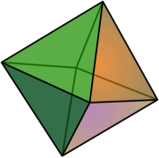
Figure 1: Cube and octahedron (www.wikipedia.org)

Example 1.9.

Figure 2: Dodecahedron and its Schlegel digram (www.wikipedia.org)

3 Euler’s formula

Let $f_{0}$, $f_{1}$, and $f_{2}$ be numbers of vertices, edges, and $2$-faces of a $3$-polytope. Leonard Euler (1707-1783) proved the following fundamental relation:

$$f_{0}-f_{1}+f_{2}=2$$

By a fragment we mean a subset $W\subset P$ that is a union of faces of $P$. Define an Euler characteristics of $W$ by

$$\chi(W)=f_{0}(W)-f_{1}(W)+f_{2}(W).$$

If $W_{1}$ and $W_{2}$ are fragments, then $W_{1}\cup W_{2}$ and $W_{1}\cap W_{2}$ are fragments.

Exercise: Proof the inclusion-exclusion formula

$$\chi(W_{1}\cup W_{2})=\chi(W_{1})+\chi(W_{2})-\chi(W_{1}\cap W_{2}),$$

4 Platonic solids

Definition 1.10.

A regular polytope (Platonic solid) [13] is a convex $3$-polytope with all facets being congruent regular polygons that are assembled in the same way around each vertex.

There are only $5$ Platonic solids, see Fig. 3.

Cube $(8,12,6)$ Dodecahedron $(20,30,12)$

Tetrahedron $(4,6,4)$

Octahedron $(6,12,8)$ Icosahedron $(12,30,20)$

Figure 3: Platonic solids with $f$-vectors $(f_{0},f_{1},f_{2})$ (www.wikipedia.org)

All Platonic solids are vertex-, edge-, and facet-transitive. They are not combinatorially chiral.

5 Archimedean solids

Definition 1.11.

An Archimedean solid [13] is a convex $3$-polytope with all facets – regular polygons of two or more types, such that for any pair of vertices there is a symmetry of the polytope that moves one vertex to another.

There are only $13$ solids with this properties: $10$ with facets of two types, and $3$ with facets of three types. On the following figures we present Archimedean solids. For any polytope we give vectors $(f_{0},f_{1},f_{2})$ and $(k_{1},\dots,k_{p};q)$, where $q$ is the valency of any vertex and a tuple $(k_{1},\dots k_{p})$ show which $k$-gons are present.

Cuboctahedron		Icosidodecahedron
$(12,24,14),(3,4;4)$		$(30,60,32),(3,5;4)$

Truncated tetrahedron	Truncated octahedron	Truncated icosahedron
$(12,18,8),(3,6;3)$	$(24,36,14),(4,6;3)$	$(60,90,32),(5,6;3)$

Truncated cube		Truncated dodecahedron
$(24,36,14),(3,8;3)$		$(60,90,32),(3,10;3)$

Rhombicuboctahedron		Rhombicosidodecahedron
$(24,48,26),(3,4;4)$		$(60,120,62),(3,4,5;4)$

Truncated		Truncated
cuboctahedron		icosidodecahedron
$(48,72,26),(4,6,8;3)$		$(120,180,62),(4,6,10;3)$

Snub cube	Snub dodecahedron
$(24,60,38),(3,4;5)$	$(60,150,92),(3,5;5)$

Figure 4: Archimedean solids with $f$-vectors and facet-vertex types (www.wikipedia.org)

Snub cube and snub dodecahedron are combinatorially chiral, while other $11$ Archimedean solids are not combinatorially chiral.

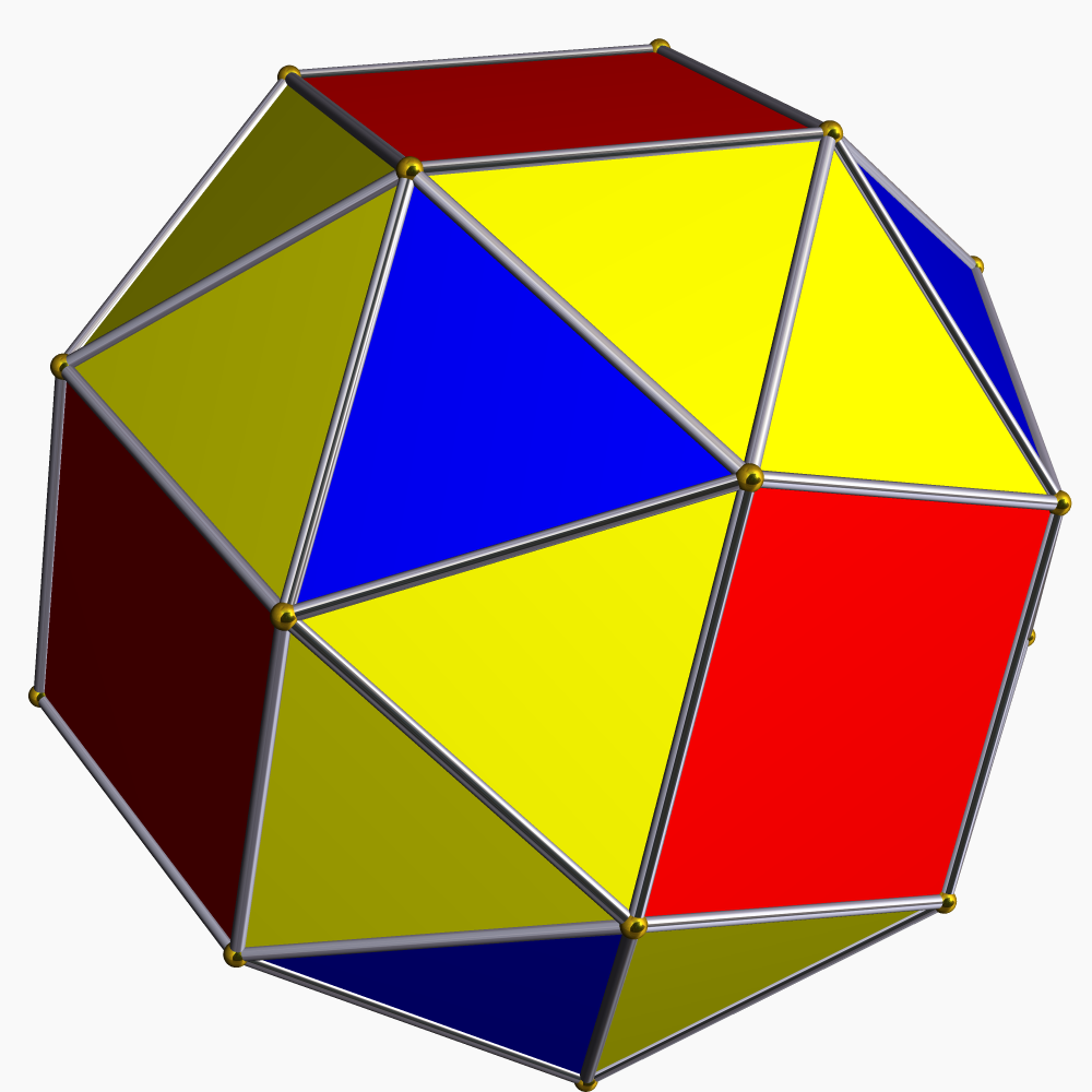
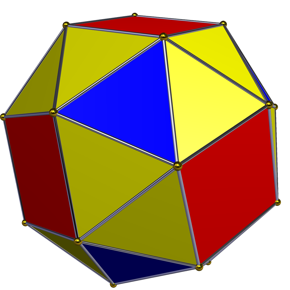
Figure 5: Left and right snub cube. Fix the orientations induced from ambient space. There is no combinatorial equivalence preserving this orientation. (www.wikipedia.org)

6 Simple polytopes

An $n$-polytope is simple if any its vertex is contained in exactly $n$ facets.

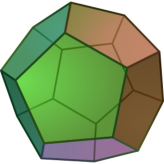
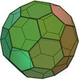
Figure 6: Simple polytopes: cube, dodecahedron and truncated icosahedron (www.wikipedia.org)

Example 1.12.

$3$ of $5$ Platonic solids are simple.

$7$ of $13$ Archimedean solids are simple.

Exercise:

A simple $n$-polytope with all $2$-faces triangles is combinatorially equivalent to the $n$-simplex.

A simple $n$-polytope with all $2$-faces quadrangles is combinatorially equivalent to the $n$-cube.

A simple $3$-polytope with all $2$-faces pentagons is combinatorially equivalent to the dodecahedron.

7 Realization of $f$-vector

Theorem 1.13.

[41] (Ernst Steinitz (1871-1928)) An integer vector $(f_{0},f_{1},f_{2})$ is a face vector of a three-dimensional polytope if and only if

$$f_{0}-f_{1}+f_{2}=2,\quad f_{2}\leqslant 2f_{0}-4,\quad f_{0}\leqslant 2f_{2}-4.$$

Corollary 1.14.

$$f_{2}+4\leqslant 2f_{0}\leqslant 4f_{2}-8$$

Well-known $g$-theorem [40, 1] gives the criterion when an integer vector $(f_{0},\dots,f_{n-1})$ is an $f$-vector of a simple $n$-polytope (see also [7]).

For general polytopes the are only partial results about $f$-vectors.

Classical problem: For four-dimensional polytopes the conditions characterizing the face vector $(f_{0},f_{1},f_{2},f_{3})$ are still not known [46].

8 Dual polytopes

For an $n$-polytope $P\subset\mathbb{R}^{n}$ with $\mathbf{0}\in{\rm int}\,P$ the dual polytope $P^{*}$ is

$$P^{*}=\{\boldsymbol{y}\in\mathbb{(}R^{n})^{*}\colon\boldsymbol{y}\boldsymbol{x}+1\geqslant 0\}$$

$i$-faces of $P^{*}$ are in an inclusion reversing bijection with $(n-i-1)$-faces of $P$.

$(P^{*})^{*}=P$. An $n$-polytope is simplicial if any its facet is a simplex.

Lemma 1.15.

A polytope dual to a simple polytope is simplicial.
A polytope dual to a simplicial polytope is simple.

Lemma 1.16.

Let a polytope $P^{n}$, $n\geqslant 2$, be simple and simplicial. Then either $n=2$, or $P^{n}$ is combinatorially equivalent to a simplex $\Delta^{n}$, $n>2$.

Example 1.17.

Among $5$ Platonic solids the tetrahedron is self-dual, the cube is dual to the octahedron, and the dodecahedron is dual to the icosahedron.

There are no simplicial polytope among Archimedean solids. Polytopes dual to Archimedean solids are called Catalan solids, since they where first described by E.C. Catalan (1814-1894). For example, the polytope dual to truncated icosahedron is called pentakis dodecahedron.

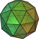
Figure 7: Truncated icosahedron and pentakis dodecahedron (www.wikipedia.org)

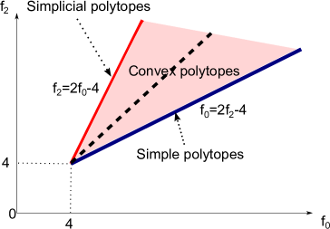
Figure 8: By Steinitz’s theorem and Euler’s formula integer points inside the cone are in the one-to-one correspondence with $f$-vectors of convex $3$-polytopes

On Fig. 8 the point $(4,4)$ corresponds to the tetrahedron. The bottom ray corresponds to simple polytopes, the upper ray – to simplicial. For $k\geqslant 3$ self-dual pyramids over $k$-gons give points on the diagonal.

9 $k$-belts

Definition 1.18.

Let $P$ be a simple convex $3$-polytope. A thick path is a sequence of facets $(F_{i_{1}},\dots,F_{i_{k}})$ with $F_{i_{j}}\cap F_{i_{j+1}}\neq\varnothing$ for $j=1,\dots,k-1$. A $k$-loop is a cyclic sequence $(F_{i_{1}},\dots,F_{i_{k}})$ of facets, such that $F_{i_{1}}\cap F_{i_{2}}$, $\dots$, $F_{i_{k-1}}\cap F_{i_{k}}$, $F_{i_{k}}\cap F_{i_{1}}$ are edges. A $k$-loop is called simple, if facets $(F_{i_{1}},\dots,F_{i_{k}})$ are pairwise different.

Example 1.19.

Any vertex of $P$ is surrounded by a simple $3$-loop. Any edge is surrounded by a simple $4$-loop. Any $k$-gonal facet is surrounded by a simple $k$-loop.

Definition 1.20.

A $k$-belt is a $k$-loop, such that $F_{i_{1}}\cap\dots\cap F_{i_{k}}=\varnothing$ and $F_{i_{p}}\cap F_{i_{q}}\neq\varnothing$ if and only if $\{p,q\}\in\{\{1,2\},\dots,\{k-~{}1,k\},\{k,1\}\}$.

Figure 9: $4$-belt of a simple $3$-polytope

10 Simple paths and cycles

By $G(P)$ we denote a vertex-edge graph of a simple $3$-polytope $P$. We call it
the graph of a polytope. Let $G$ be a graph.

Definition 1.21.

An edge path is a sequence of vertices $(v_{1},\dots,v_{k})$, $k>1$ such that $v_{i}$ and $v_{i+1}$ are connected by some edge $E_{i}$ for all $i<k$.

An edge path is simple if it passes any vertex of $G$ at most once.

A cycle is a simple edge path, such that $v_{k}=v_{1}$, where $k>2$. We denote a cycle by $(v_{1},\dots,v_{k-1})$.

A cycle $(v_{1},\dots,v_{k})$ in the graph of a simplicial $3$-polytope $P$ is dual to a $k$-belt in a simple $3$-polytope $P^{*}$ if all it’s vertices do not lie in the same face, and $v_{i}$ and $v_{j}$, are connected by an edge if and only if $\{i,j\}\in\{\{1,2\},\dots,\{k-1,k\},\{k,1\}\}$.

Figure 10: $(F_{i},F_{j},F_{k})$ is a $3$-belt  $(v_{i},v_{j},v_{k})$ is a cycle dual to the $3$-belt

Definition 1.22.

A zigzag path on a simple $3$-polytope is an edge path with no $3$ successive edges lying in the same facet.

Starting with one edge an choosing the second edge having with it a common vertex, we obtain a unique way to construct a zigzag.

Definition 1.23.

A zigzag cycle on a simple $3$-polytope is a cycle with no $3$ successive edges lying in the same facet.

Figure 11: A zigzag cycle on the Schlegel diagram of the dodecahedron

11 The Steinitz theorem

Definition 1.24.

A graph $G$ is called simple if it has no loops and multiple edges. A connected graph $G$ is called $3$-connected, if it has at least $6$ edges and deletion of any one or two vertices with all incident edges leaves $G$ connected.

Theorem 1.25.

(The Steinitz theorem, see [47])
A graph $G$ is a graph of a $3$-polytope if and only if it is simple, planar and $3$-connected.

Remark 1.26.

Moreover, the cycles in $G$ corresponding to facets are exactly chordless simple edge cycles $C$ with $G\setminus C$ disconnected; hence the combinatorics of the embedding $G\subset S^{2}$ is uniquely defined.

We will need the following version of the Jordan curve theorem. It can be proved rather directly similarly to the piecewise-linear version of this theorem on the plane.

Theorem 1.27.

Let $\gamma$ be a simple piecewise-linear (in respect to some homeomorphism $S^{2}\simeq\partial P$ for a $3$-polytope $P$) closed curve on the sphere $S^{2}$. Then

1. $S^{2}\setminus\gamma$ consists of two connected components $\mathcal{C}_{1}$ and  $\mathcal{C}_{2}$.

2. Closure $\overline{\mathcal{C}_{\alpha}}$ is homeomorphic to a disk for each $\alpha=1,2$.

We will also need the following result.

Lemma 1.28.

Let $G\subset S^{2}$ be a finite simple graph with at least $6$ edges. Then $G$ is $3$-connected if and only if all connected components of $S^{2}\setminus G$ are bounded by simple edge cycles and closures of any two areas (<<facets>>) either do not intersect, or intersect by a single common vertex, or intersect by a single common edge.

Proof 1.29.

Let $G$ satisfy the condition of the lemma. We will prove that $G$ is $3$-connected. Let $v_{1}\neq v_{2}$, $u_{1},u_{2}\notin\{v_{1},v_{2}\}$, be vertices of $G$, perhaps $u_{1}=u_{2}$. We need to prove that there is an edge-path from $v_{1}$ to $v_{2}$ in $G\setminus\{u_{1},u_{2}\}$. Since $G$ is connected, there is an edge-path $\gamma$ connecting $v_{1}$ and $v_{2}$. Consider the vertex $u_{\alpha}$, $\alpha\in\{1,2\}$, and all facets $F_{i_{1}},\dots,F_{i_{p}}$ containing it. From the hypothesis of the lemma $p\geqslant 3$. Since the graph is embedded to the sphere, after relabeling we obtain a simple $p$-loop $(F_{i_{1}},\dots,F_{i_{p}})$. For $j=\in\{1,\dots,p\}$ denote by $w_{j}$ the end of the edge $F_{i_{j}}\cap F_{i_{j+1}}$ different from $u_{\alpha}$, where $F_{i_{p+1}}=F_{i_{1}}$. Let $g_{j}$ be the simple edge-path connecting $w_{j-1}$ and $w_{j}$ in $F_{i_{j}}\setminus u_{\alpha}$ (See Fig. 12).

Figure 12: Star of the vertex $u_{\alpha}$

Then $\eta_{\alpha}=(g_{1},g_{2},\dots,g_{p})$ is a simple edge-cycle. Indeed, if $g_{s}$ and $g_{t}$ have common vertex, then this vertex belongs to $F_{i_{s}}\cap F_{i_{t}}$ together with $u_{\alpha}$; hence it is connected with $u_{\alpha}$ by an edge; therefore $\{s,t\}=\{k,k+1\mod p\}$ for some $k$, and the vertex is $w_{k}$. If $u_{1}$ and $u_{2}$ are different and are connected by an edge $E$, then $E=F_{i_{s}}\cap F_{i_{t}}$ for some $s,t\in\{1,\dots,p\}$, $s-t=\pm 1\mod p$, and we can change $\gamma$ not to contain $E$ substituting the simple edge-path in $F_{i_{s}}\setminus E$ for $E$. Now for the new path $\gamma_{1}$ consider all times it passes $u_{\alpha}$. We can remove all the fragments $(w_{i},u_{\alpha},w_{j})$ and substitute the simple edge path in $\eta_{\alpha}\setminus u_{\beta}$ connecting $w_{i}$ and $w_{j}$ for each fragment $(w_{i},u_{\alpha},w_{j})$. The same can be done for $u_{\beta}$, $\{\alpha,\beta\}=\{1,2\}$. Thus we obtain the edge-path $\gamma_{2}$ connecting $v_{1}$ and $v_{2}$ in $G\setminus\{u_{1},u_{2}\}$.

Now let $G$ be $3$-connected. Consider the connected component $D$ of $S^{2}\setminus G$ and it’s boundary $\partial D$. If there is a hanging vertex $v\in\partial D$ of $G$, then deletion of the other end of the edge containing $v$ makes the graph disconnected. Hence any vertex $v\in\partial D$ of $G$ gas valency at least $2$, and $D$ is surrounded by an edge-cycle $\eta$. If $\eta$ is not simple, then there is a vertex $v\in\eta$ passed several times. Then the area $D$ appears several times when we walk around the vertex $v$. Since $D$ is connected, there is a simple piecewise-linear (in respect to some homeomorphism $S^{2}\simeq\partial P$ for a $3$-polytope $P$) closed curve $\eta$ in the closure $\overline{D}$ of $D$ with the only point $v$ on the boundary. Walking round $v$, we pass edges in both connected component of $S^{2}\setminus\eta$; hence the deletion of $v$ divides $G$ into several connected components. Thus the cycle $\eta$ is simple. Let facets $F_{1}=\overline{D_{1}}$, $F_{2}=\overline{D_{2}}$ have two common vertices $v_{1}$, $v_{2}$. Consider piecewise linear simple curves $\eta_{1}\subset F_{1}$, $\eta_{2}\subset F_{2}$, with ends $v_{1}$ and $v_{2}$ and all other points lying in $D_{1}$ and $D_{2}$ respectively. Then $\eta_{1}\cup\eta_{2}$ is a simple piecewise-linear closed curve; hence it separates the sphere $S^{2}$ into two connected components. If $v_{1}$ and $v_{2}$ are not adjacent in $F_{1}$ or $F_{2}$, then both connected components contain vertices of $G$; hence deletion of $v_{1}$ and $v_{2}$ makes the graph disconnected. Thus any two common vertices are adjacent in both facets. Moreover, since there are no multiple edges, the corresponding edges belong to both facets. Then either both facets are surrounded by a common $3$-cycle, and in this case $G$ has only $3$ edges, or any two facets either do not intersect, or intersect by a common vertex, or intersect by a common edge. This finishes the proof.

Let $\mathcal{L}_{k}=(F_{i_{1}},\dots,F_{i_{k}})$ be a simple $k$-loop for $k\geqslant 3$. Consider midpoints $w_{j}$ of edges $F_{i_{j}}\cap F_{i_{j+1}}$, $F_{i_{k+1}}=F_{i_{1}}$ and segments $E_{j}$ connecting $w_{j}$ and $w_{j+1}$ in $F_{j+1}$. Then $(E_{1},\dots,E_{k})$ is a simple piecewise-linear curve $\eta$ on $\partial P$. It separates $\partial P\simeq S^{2}$ into two areas homeomorphic to discs $D_{1}$ and $D_{2}$ with $\partial D_{1}=\partial D_{2}=\eta$. Consider two graphs $G_{1}$ and $G_{2}$ obtained from the graph $G(P)$ of $P$ by addition of vertices $\{w_{j}\}_{j=1}^{k}$ and edges $\{E_{j}\}_{j=1}^{k}$, and deletion of all vertices and edges with interior points inside $D_{1}$ or $D_{2}$ respectively.

Lemma 1.30.

There exist simple polytopes $P_{1}$ and $P_{2}$ with graphs $G_{1}=G(P_{1})$ and $G_{2}=G(P_{2})$.

Proof 1.31.

The proof is similar for both graphs; hence we consider the graph $G_{1}$. It has at least $6$ edges, is connected and planar. Now it is sufficient to prove that the hypothesis of Lemma 1.28 is valid. For this we see each facet of $G_{1}$ is either a facet of $P$, or it is a part of a facet $F_{i_{j}}$ for some $j$, or it is bounded by the cycle $\eta$. In particular, all facets are bounded by simple edge-cycles. If the facets $F_{i}$ and $F_{j}$ are both of the first two types they either do not intersect or intersect by common edge as it is in $P$. If $F$ is the facet bounded by $\eta$, then it intersects only facets $(F_{i_{1}},\dots,F_{i_{k}})$, and each intersection is an edge $F\cap F_{i_{j}}$, $j=1,\dots,k$.

Definition 1.32.

We will call polytopes $P_{1}$ and $P_{2}$ loop-cuts (or, more precisely, $\mathcal{L}_{k}$-cuts) of $P$.

2 Lecture 2. Combinatorics of simple polytopes

1 Flag polytopes

Definition 2.1.

A simple polytope is called flag if any set of pairwise intersecting facets $F_{i_{1}},\dots,F_{i_{k}}$: $F_{i_{s}}\cap F_{i_{t}}\neq\varnothing$, $s,t=1,\dots,k$, has a nonempty intersection $F_{i_{1}}\cap\dots\cap F_{i_{k}}\neq\varnothing$.

a)		b)

Figure 13: a) flag polytope; b) non-flag polytope (www.wikipedia.org)

Example 2.2.

$n$-simplex $\Delta^{n}$ is not a flag polytope for $n\geqslant 2$.

Proposition 2.3.

Simple $3$-polytope $P$ is not flag if and only if either $P=\Delta^{3}$, or $P$ contains a $3$-belt.

Corollary 2.4.

Simple $3$-polytope $P\neq\Delta^{3}$ is flag if and only any $3$-loop corresponds to a vertex.

Proposition 2.5.

Simple $3$-polytope $P$ is flag if and only if any facet is surrounded by a $k$-belt, where $k$ is the number of it’s edges.

Proof 2.6.

A simplex is not flag and has no $3$-belts.

By Proposition 2.3 a simple $3$-polytope $P\not\simeq\Delta^{3}$ is not flag if and only if it has a $3$-belt. The facet $F\subset P$ is not surrounded by a belt if and only if it belongs to a $3$-belt.

Corollary 2.7.

For any flag simple $3$-polytope $P$ we have $p_{3}=0$.

Later (see Lecture 9) we will need the following result.

Proposition 2.8.

A flag $3$-polytope $P$ has no $4$-belts if and only if any pair of adjacent facets is surrounded by a belt.

Proof 2.9.

The pair $(F_{i},F_{j})$ of adjacent facets is a $2$-loop and is surrounded by a simple edge-cycle. Let $\mathcal{L}=(F_{i_{1}},\dots,F_{i_{k}})$ be the $k$-loop that borders it. If $\mathcal{L}$ is not simple, then $F_{i_{a}}=F_{i_{b}}$ for $a\neq b$. Then $F_{i_{a}}$ and $F_{i_{b}}$ are not adjacent to the same facet $F_{i}$ or $F_{j}$. Let $F_{i_{a}}$ be adjacent to $F_{i}$, and $F_{i_{b}}$ to $F_{j}$. Then $(F_{i},F_{j},F_{i_{a}})$ is a $3$-belt. A contradiction. Hence $\mathcal{L}$ is a simple loop. If it is not a belt, then $F_{i_{a}}\cap F_{i_{b}}\neq\varnothing$ for non-successive facets $F_{i_{a}}$ and $F_{i_{b}}$. From Proposition 2.5 we obtain that $F_{i_{a}}$ and $F_{i_{b}}$ are not adjacent to the same facet $F_{i}$ or $F_{j}$. Let $F_{i_{a}}$ be adjacent to $F_{i}$, and $F_{i_{b}}$ to $F_{j}$. Then $(F_{i_{a}},F_{i},F_{j},F_{i_{b}})$ is a $4$-belt. On the other hand, if there is a $4$-belt $(F_{i},F_{j},F_{k},F_{l})$, then facets $F_{k}$ and $F_{l}$ belong to the loop surrounding the pair $(F_{i},F_{j})$. Since $F_{i}\cap F_{k}=\varnothing=F_{j}\cap F_{l}$, they are not successive facets of this loop; hence the loop is not a belt. This finishes the proof.

In the combinatorial study of fullerenes the following version of the Jordan curve theorem gives the important tool. It follows from the Theorem 1.27.

Theorem 2.10.

Let $\gamma$ be a simple edge-cycle on a simple $3$-polytope $P$. Then

1. $\partial P\setminus\gamma$ consists of two connected components $\mathcal{C}_{1}$ and  $\mathcal{C}_{2}$.

2. Let $\mathcal{D}_{\alpha}=\{F_{j}\in\mathcal{F}_{P}\colon{\rm int}\,F_{j}\subset\mathcal{C}_{\alpha}\}$, $\alpha=1,2$. Then $\mathcal{D}_{1}\sqcup\mathcal{D}_{2}=\mathcal{F}_{P}$.

3. The closure $\overline{\mathcal{C}_{\alpha}}$ is homeomorphic to a disk. We have $\overline{\mathcal{C}_{\alpha}}=|\mathcal{D}_{\alpha}|$.

Corollary 2.11.

If we remove the $3$-belt from the surface of a simple $3$-polytope, we obtain two parts $W_{1}$ and $W_{2}$, homeomorphic to disks.

Figure 14: $3$-belt on the surface of a simple $3$-polytope

Proposition 2.12.

Let $P$ be a flag simple $3$-polytope. Then $m\geqslant 6$, and $m=6$ if and only if $P$ is combinatorially equivalent to the cube $I^{3}$.

Proof 2.13.

Take a facet $F_{1}$. By Proposition 2.5 it is surrounded by a $k$-belt $\mathcal{B}=(F_{i_{1}},\dots,F_{i_{k}})$, $k\geqslant 4$. Since there is at least one facet in the connected component $W_{\alpha}$ of $\partial P\setminus\mathcal{B}$, ${\rm int\,}F_{1}\notin W_{\alpha}$, we obtain $m\geqslant 2+k\geqslant 6$. If $m=6$, then $k=4$, $F_{1}$ is a quadrangle, and $W_{\alpha}={\rm int\,}F_{j}$ for some facet $F_{j}$ Then $F_{j}\cap F_{i_{1}}\cap F_{i_{2}}$, $F_{j}\cap F_{i_{2}}\cap F_{i_{3}}$, $F_{j}\cap F_{i_{3}}\cap F_{i_{4}}$, $F_{j}\cap F_{i_{4}}\cap F_{i_{1}}$ are vertices, and $P$ is combinatorially equivalent to $I^{3}$.

Lemma 2.14.

Let $P$ be a flag polytope, $\mathcal{L}_{k}$ be a simple $k$-loop, and $P_{1}$ and $P_{2}$ be $\mathcal{L}_{k}$-cuts of $P$. Then the following conditions are equivalent:

1. both polytopes $P_{1}$ and $P_{2}$ are flag;

2. $\mathcal{L}_{k}$ is a $k$-belt.

Proof 2.15.

Since $P$ has no $3$-belts, for $k=3$ the loop $\mathcal{L}_{k}$ surrounds a vertex; hence one of the polytopes $P_{1}$ and $P_{2}$ is a simplex, and it is not flag. Let $k\geqslant 4$. Then $P_{1}$ and $P_{2}$ are not simplices. There are three types of facets in $P$: lying only in $P_{1}$, lying only in $P_{2}$, and lying in $\mathcal{L}_{k}$. Let $\mathcal{B}_{3}=(F_{i},F_{j},F_{k})$ be a $3$-loop in $P_{\alpha}$, $\alpha\in\{1,2\}$. Let $F_{i},F_{j},F_{k}$ correspond to facets of $P$. Since intersecting facets in $P_{\alpha}$ also intersect in $P$, $(F_{i},F_{j},F_{k})$ is also a $3$-loop in $P$, and $F_{i}\cap F_{j}\cap F_{k}\in P$ is a vertex. Since $F_{i}\cap F_{j}\neq\varnothing$ in $P_{\alpha}$, either the corresponding edge of $P$ lies in $P_{\alpha}$, or it intersects the new facet, and $F_{i}$ and $F_{j}$ are consequent facets of $\mathcal{L}_{k}$. Since $k\geqslant 4$, at least one edge of $F_{i}\cap F_{j}$, $F_{j}\cap F_{k}$, and $F_{k}\cap F_{i}$ of $P$ lies in $P_{\alpha}$; hence $F_{i}\cap F_{j}\cap F_{k}\in P_{\alpha}$, and $\mathcal{B}_{3}$ is not a $3$-belt in $P_{\alpha}$. If one of the facets, say $F_{i}$, is a new facet of $P_{\alpha}$, then $F_{j},F_{k}\in\mathcal{L}_{k}$, since $F_{i}\cap F_{j},F_{i}\cap F_{k}\neq\varnothing$. Consider the edge $F_{j}\cap F_{k}$ of $P$. It intersects $F_{i}$ in $P_{\alpha}$ if and only if $F_{j}$ and $F_{k}$ are consequent facets in $\mathcal{L}_{k}$. Thus if $\mathcal{B}_{3}$ is a $3$-belt, then $\mathcal{L}_{k}$ is not a $k$-belt, and vice versa, if $\mathcal{L}_{k}$ is not a $k$-belt, then $F_{j}\cap F_{k}\neq\varnothing$ for some non-consequent facets of $\mathcal{L}_{k}$, and the corresponding $3$-loop $\mathcal{B}_{3}$ is a $3$-belt in the polytope $P_{1}$ or $P_{2}$ containing $F_{j}\cap F_{k}$. This finishes the proof.

2 Non-flag $3$-polytopes as connected sums

The existence of a $3$-belt is equivalent to the fact that $P$ is combinatorially equivalent to a connected sum $P=Q_{1}\#_{v_{1},v_{2}}Q_{2}$ of two simple $3$-polytopes $Q_{1}$ and $Q_{2}$ along vertices $v_{1}$ and $v_{2}$.

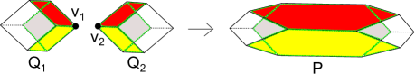
Figure 15: Connected sum of two simple polytopes along vertices

The part $W_{i}$ appears if we remove from the surface of the polytope $Q_{i}$ the facets containing the vertex $v_{i}$, $i=1,2$.

3 Consequence of Euler’s formula for simple $3$-polytopes

Let $p_{k}$ be a number of $k$-gonal facets of a $3$-polytope.

Theorem 2.16.

(See [27]) For any simple $3$-polytope $P$

$$3p_{3}+2p_{4}+p_{5}=12+\sum\limits_{k\geqslant 7}(k-6)p_{k},$$ (1)

Proof 2.17.

The number of pairs (edge, vertex of this edge) is equal, on the one hand, to $2f_{1}$ and, on the other hand (since the polytope is simple), to $3f_{0}$. Then $f_{0}=\frac{2f_{1}}{3}$, and from the Euler formula we obtain $2f_{1}=6f_{2}-12$. Counting the pairs (facet, edge of this facet), we have

$$\sum\limits_{k\geqslant 3}kp_{k}=2f_{1}=6\left(\sum\limits_{k\geqslant 3}p_{k}\right)-12,$$

which implies formula (1).

Corollary 2.18.

There is no simple polytope $P$ with all facets hexagons. Moreover, if $p_{k}=0$ for $k\neq 5,6$, then $p_{5}=12$.

Exercise: The $f$-vector of a simple polytope is expressed in terms of the $p$-vector by the following formulas:

$$f_{0}=2\left(f_{2}-2\right)\quad f_{1}=3\left(f_{2}-2\right)\quad f_{2}=\sum_{k}p_{k}$$

4 Realization theorems

Definition 2.19.

An integer sequence $(p_{k}|k\geqslant 3)$ is called $3$-realizable is there is a simple $3$-polytope $P$ with $p_{k}(P)=p_{k}$.

Theorem 2.20.

(Victor Eberhard [20], see [27]) For a sequence $(p_{k}|3\leqslant k\neq 6)$ there exists $p_{6}$ such that the sequence $(p_{k}|k\geqslant 3)$ is $3$-realizable if and only if it satisfies formula (1) .

There arise a natural question.

Problem: For a given sequence $(p_{k}|3\leqslant k\neq 6)$ find all $p_{6}$ such that the sequence $(p_{k}|k\geqslant 3)$ is $3$-realizable.
Notation: When we write a finite sequence $(p_{3},p_{4},\dots,p_{k})$ we mean that $p_{l}=0$ for $l>k$.

Example 2.21.

(see [27]) Sequences $(0,6,0,p_{6})$ and $(0,0,12,p_{6})$ are $3$-realizable if and only if $p_{6}\neq 1$. The sequence $(4,0,0,p_{6})$ is $3$-realizable if and only if $p_{6}$ is an even integer different from $2$. The sequence $(3,1,1,p_{6})$ is $3$-realizable if and only if $p_{6}$ is an odd integer greater than $1$.

Let us mention also the following results.

Theorem 2.22.

For a given sequence $(p_{k}|3\leqslant k\neq 6)$ satisfying formula (1)

there exists $p_{6}\leqslant 3\left(\sum\limits_{k\neq 6}p_{k}\right)$ such that the sequence $(p_{k}|k\geqslant 3)$ is $3$-realizable [25];

if $p_{3}=p_{4}=0$ then any sequence $(p_{k}|k\geqslant 3,p_{6}\geqslant 8)$ is $3$-realizable [26].

There are operations on simple $3$-polytopes that do not effect $p_{k}$ except for $p_{6}$. We call them $p_{6}$-operations. As we will see later they are important for applications.

Operation I: The operation affects all edges of the polytope $P$. We present a fragment on Fig. 16.

Figure 16: Operation I

On the right picture the initial polytope $P$ is drawn by dotted lines, while the resulting polytope – by solid lines. We have

$$p_{k}(P^{\prime})=\begin{cases}p_{k}(P),&k\neq 6;\\ p_{6}(P)+f_{1}(P),&k=6.\end{cases}$$

Operation II: The operation affects all edges of the polytope $P$. We present a fragment on Fig. 17.

Figure 17: Operation II

On the right picture the initial polytope $P$ is drawn by dotted lines, while the resulting polytope – by solid lines. We have

$$p_{k}(P^{\prime})=\begin{cases}p_{k}(P),&k\neq 6;\\ p_{6}(P)+f_{0}(P),&k=6.\end{cases}$$

Operation I and Operation II are called iterative procedures (see [33]), since arbitrary compositions of them are well defined.

Exercise: Operation I and Operation II commute; therefore they define an action of the semigroup $\mathbb{Z}_{\geqslant 0}\times\mathbb{Z}_{\geqslant 0}$ on the set of all combinatorial simple $3$-polytopes, where $\mathbb{Z}_{\geqslant 0}$ is the additive semigroup of nonnegative integers.

5 Graph-truncation of simple $3$-polytopes

Consider a subgraph $\Gamma\subset G(P)$ without isolated vertices. For each edge

$$E_{i,j}=F_{i}\cap F_{j}=P\cap\{\boldsymbol{x}\in\mathbb{R}^{3}\colon(\boldsymbol{a}_{i}+\boldsymbol{a}_{j})\boldsymbol{x}+(b_{i}+b_{j})=0\}$$

consider the halfspace

$$\mathcal{H}_{ij,\varepsilon}^{+}=\{\boldsymbol{x}\in\mathbb{R}^{3}\colon(\boldsymbol{a}_{i}+\boldsymbol{a}_{j})\boldsymbol{x}+(b_{i}+b_{j})\geqslant\varepsilon\}.$$

Set

$$P_{\Gamma,\varepsilon}=P\cap\bigcap\limits_{E_{i,j}\in\Gamma}\mathcal{H}^{+}_{ij,\varepsilon}$$

Exercise: For small enough values of $\varepsilon$ the combinatorial type of $P_{\Gamma,\varepsilon}$ does not depend on $\varepsilon$.

Definition 2.23.

We will denote by $P_{\Gamma}$ the combinatorial type of $P_{\Gamma,\varepsilon}$ for small enough values of $\varepsilon$ and call it a $\Gamma$-truncation of $P$. When it is clear what is $\Gamma$ we call $P_{\Gamma}$ simply graph-truncation of $P$.

Example 2.24.

For $\Gamma=G(P)$ the polytope $P^{\prime}=P_{\Gamma}$ is obtained from $P$ by a $p_{6}$-operation I defined above.

Proposition 2.25.

Let $P$ be a simple polytope with $p_{3}=0$. Then the polytope $P_{G(P)}$ is flag.

We leave the proof as an exercise.

Corollary 2.26.

For a given sequence $(p_{k}|3\leqslant k\neq 6)$ satisfying formula (1) there are infinitely many values of $p_{6}$ such that the sequence $(p_{k}|k\geqslant 3)$ is $3$-realizable.

6 Analog of Eberhard’s theorem for flag polytopes

Theorem 2.27.

[9] For every sequence $(p_{k}|3\leqslant k\neq 6,p_{3}=0)$ of nonnegative integers satisfying formula (1) there exists a value of $p_{6}$ such that there is a flag simple $3$-polytope $P^{3}$ with $p_{k}=p_{k}(P^{3})$ for all $k\geqslant 3$.

Proof 2.28.

For a given sequence $(p_{k}|3\leqslant k\neq 6,p_{3}=0)$ satisfying formula (1) by Eberhard’s theorem there exists a simple polytope $P$ with $p_{k}=p_{k}(P)$, $k\neq 6$. Then the polytope $P^{\prime}=P_{G(P)}$ is flag by Proposition 2.25. We have $p_{k}(P^{\prime})=p_{k}(P)$, $k\neq 6$, and $p_{6}(P^{\prime})=p_{6}(P)+f_{1}(P)$.

3 Lecture 3. Combinatorial fullerenes

1 Fullerenes

A fullerene is a molecule of carbon that is topologically sphere and any atom belongs to exactly three carbon rings, which are pentagons or hexagons.

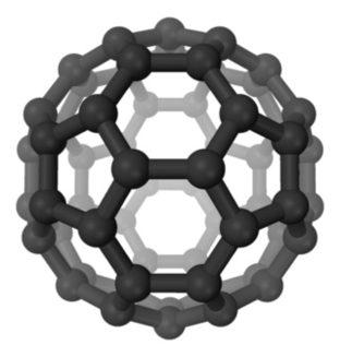
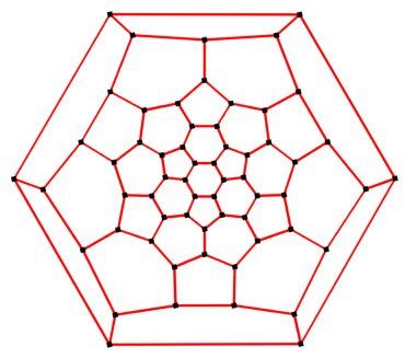
Buckminsterfullerene $C_{60}$	Schlegel diagram
$(f_{0},f_{1},f_{2})=(60,90,32)$
$(p_{5},p_{6})=(12,20)$

Figure 18: Buckminsterfullerene and it’s Schlegel diagram (www.wikipedia.org)

The first fullerene $C_{60}$ was generated by chemists-theorists Robert Curl, Harold Kroto, and Richard Smalley in 1985 (Nobel Prize in chemistry 1996, [14, 31, 39]). They called it Buckminsterfullerene.

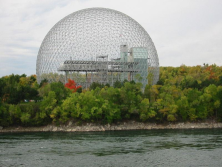
Fullerenes were named after Richard Buckminster Fuller (1895-1983) – a famous american architect, systems theorist, author, designer and inventor. In 1954 he patented an architectural construction in the form of polytopal spheres for roofing large areas. They are also called buckyballs.

Figure 19: Fuller’s Biosphere, USA Pavillion on Expo-67 (Montreal, Canada) (www.wikipedia.org)

Definition 3.1.

A combinatorial fullerene is a simple $3$-polytope with all facets pentagons and hexagons.

To be short by a fullerene below we mean a combinatorial fullerene.

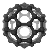
Figure 20: Fullerene $C_{60}$ and truncated icosahedron (www.wikipedia.org)

For any fullerene $p_{5}=12$, and expression of the $f$-vector in terms of the $p$-vector obtains the form

$$f_{0}=2(10+p_{6}),\quad f_{1}=3(10+p_{6}),\quad f_{2}=(10+p_{6})+2$$

Remark 3.2.

Since the combinatorially chiral polytope is geometrically chiral (see Proposition 1.6), the following problem is important for applications in the physical theory of fullerenes:

Problem: To find an algorithm to decide if the given fullerene is combinatorially chiral.

2 Icosahedral fullerenes

Operations I and II (see page 2.22) transform fullerenes into fullerenes. The first procedure increases $f_{0}$ in $4$ times, the second – in $3$ times.

Applying operation I to the dodecahedron we obtain fullerene $C_{80}$ with $p_{6}=30$. In total there are $31924$ fullerenes with $p_{6}=30$.

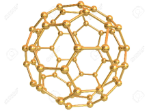
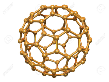
$C_{60}$	$C_{80}$

Figure 21: Icosahedral fullerenes $C_{60}$ and $C_{80}$ (http://previews.123rf.com)

Applying operation II to the dodecahedron we obtain the Buckminsterfullerene $C_{60}$ with $p_{6}=20$. In total there are $1812$ fullerenes with $p_{6}=20$.

Definition 3.3.

Fullerene with a (combinatorial) group of symmetry of the icosahedron is called an icosahedral fullerene.

The construction implies that starting from the dodecahedron any combination of the first and the second iterative procedures gives an icosahedral fullerene.
Exercise: Proof that the opposite is also true.

Denote operation $1$ by $T_{1}$ and operation $2$ by $T_{2}$. Theses operations define the action of the semigroup $\mathbb{Z}^{2}_{\geqslant 0}$ on the set of combinatorial fullerenes.

Proposition 3.4.

The operations $T_{1}$ and $T_{2}$ change the number of hexagons of the fullerene $P$ by the following rule:

$$p_{6}(T_{1}P)=30+4p_{6}(P);\quad p_{6}(T_{2}P)=20+3p_{6}(P).$$

The proof we leave as an exercise.

Corollary 3.5.

The $f$-vector of a fullerene is changed by the following rule:

$$T_{1}(f_{0},f_{1},f_{2})=(4f_{0},4f_{1},f_{2}+f_{1});\quad T_{2}(f_{0},f_{1},f_{2})=(3f_{0},3f_{1},f_{2}+f_{0}).$$

3 Cyclic $k$-edge cuts

Definition 3.6.

Let $\Gamma$ be a graph. A cyclic $k$-edge cut is a set $E$ of $k$ edges of $\Gamma$, such that $\Gamma\setminus E$ consists of two connected component each containing a cycle, and for any subset $E^{\prime}\subsetneq E$ the graph $\Gamma\setminus E^{\prime}$ is connected.

For any $k$-belt $(F_{1},\dots,F_{k})$ of the simple $3$-polytope $P$ the set of edges $\{F_{1}\cap F_{2},\dots,F_{k-1}\cap F_{k},F_{k}\cap F_{1}\}$ is a cyclic $k$-edge cut of the graph $G(P)$. For $k=3$ any cyclic $k$-edge cut in $G(P)$ is obtained from a $3$-belt in this way. For larger $k$ not any cyclic $k$-edge cut is obtained from a $k$-belt.

In the paper [18] it was proved that for any fullerene $P$ the graph $G(P)$ has no cyclic $3$-edge cuts. In [19] it was proved that $G(P)$ has no cyclic $4$-edge cuts. In [32] and [29] cyclic $5$-edge cuts were classified. In [29] cyclic $6$-edge cuts were classified. In [30] degenerated cyclic $7$-edge cuts and fullerenes with non-degenerated cyclic $7$-edge cuts were classified, where a cyclic $k$-edge cut is called degenerated, if one of the connected components has less than $6$ pentagonal facets, otherwise it is called non-degenerated.

4 Fullerenes as flag polytopes

Let $\gamma$ be a simple edge-cycle on a simple $3$-polytope. We say that $\gamma$ borders a $k$-loop $\mathcal{L}$ if $\mathcal{L}$ is a set of facets that appear when we walk along $\gamma$ in one of the components $\mathcal{C}_{\alpha}$. We say that an $l_{1}$-loop $\mathcal{L}_{1}=(F_{i_{1}},\dots,F_{i_{l_{1}}})$ borders an $l_{2}$-loop $\mathcal{L}_{2}=(F_{j_{1}},\dots,F_{j_{l_{2}}})$ (along $\gamma$), if they border the same edge-cycle $\gamma$. If $l_{2}=1$, then we say that $\mathcal{L}_{1}$ surrounds $F_{j_{1}}$.

Let $\gamma$ have $a^{1}_{p}$ successive edges corresponding to $F_{i_{p}}\in\mathcal{L}_{1}$, and $a^{2}_{q}$ successive edges corresponding to $F_{j_{q}}\in\mathcal{L}_{2}$.

Lemma 3.7.

Let a loop $\mathcal{L}_{1}$ border a loop $\mathcal{L}_{2}$ along $\gamma$. Then one of the following holds:

1. $\mathcal{L}_{\alpha}$ is a $1$-loop, and $\mathcal{L}_{\beta}$ is a $a^{\alpha}_{1}$-loop, for $\{\alpha,\beta\}=\{1,2\}$;

2. $l_{1},l_{2}\geqslant 2$, $l_{1}+l_{2}=l_{\gamma}=\sum_{r=1}^{l_{1}}a^{1}_{r}=\sum_{r=1}^{l_{2}}a^{2}_{r}$.

Proof 3.8.

If $l_{2}=1$, then $\gamma$ is a boundary of the facet $F_{j_{1}}$, successive edges of $\gamma$ belong to different facets in $\mathcal{L}_{1}$, and $l_{1}=a^{2}_{1}$. Similar argument works for $l_{1}=1$.

Let $l_{1},l_{2}\geqslant 2$. Any edge of $\gamma$ is an intersection of a facet from $\mathcal{L}_{1}$ with a facet from $\mathcal{L}_{2}$. Successive edges of $\gamma$ belong to the same facet in $\mathcal{L}_{\alpha}$ if and only if they belong to successive facets in $\mathcal{L}_{\beta}$, $\{\alpha,\beta\}=\{1,2\}$; therefore$l_{\alpha}=\sum_{r=1}^{l_{\beta}}(a^{\beta}_{r}-1)=\sum_{r=1}^{l_{\beta}}a_{r}^{\beta}-l_{\beta}$. We have $l_{\gamma}=\sum_{r=1}^{l_{\beta}}a_{r}^{\beta}=l_{1}+l_{2}$.

Lemma 3.9.

Let $\mathcal{B}=(F_{i_{1}},\dots,F_{i_{k}})$ be a $k$-belt. Then

1. $|\mathcal{B}|=F_{i_{1}}\cup\dots\cup F_{i_{k}}$ is homeomorphic to a cylinder;

2. $\partial|\mathcal{B}|$ consists of two simple edge-cycles $\gamma_{1}$ and $\gamma_{2}$.

3. $\partial P\setminus|\mathcal{B}|$ consists of two connected components $\mathcal{P}_{1}$ and $\mathcal{P}_{2}$.

4. Let $\mathcal{W}_{\alpha}=\{F_{j}\in\mathcal{F}_{P}\colon{\rm int\,}F_{j}\subset\mathcal{P}_{\alpha}\}\subset\mathcal{F}_{P}$, $\alpha=1,2$.
   Then $\mathcal{W}_{1}\sqcup\mathcal{W}_{2}\sqcup\mathcal{B}=\mathcal{F}_{P}$.

5. $\overline{\mathcal{P_{\alpha}}}=|\mathcal{W}_{\alpha}|$ is homeomorphic to a disk, $\alpha=1,2$.

6. $\partial\mathcal{P}_{\alpha}=\partial\overline{\mathcal{P}_{\alpha}}=\gamma_{\alpha}$, $\alpha=1,2$.

The proof is straightforward using Theorem 2.10.

Let a facet $F_{i_{j}}\in\mathcal{B}$ has $\alpha_{j}$ edges in $\gamma_{1}$ and $\beta_{j}$ edges in $\gamma_{2}$. If $F_{i_{j}}$ is an $m_{i_{j}}$-gon, then $\alpha_{j}+\beta_{j}=m_{i_{j}}-2$.

Lemma 3.10.

Let $P$ be a simple $3$-polytope with $p_{3}=0$, $p_{k}=0$, $k\geqslant 8$, $p_{7}\leqslant 1$, and let $\mathcal{B}_{k}$ be a $k$-belt, $k\geqslant 3$, consisting of $b_{i}$ $i$-gons, $4\leqslant i\leqslant 7$. Then one of the following holds:

1. $\mathcal{B}_{k}$ surrounds two $k$-gonal facets $F_{s}:\{F_{s}\}=\mathcal{W}_{1}$, and $F_{t}:\{F_{t}\}=\mathcal{W}_{2}$,
   and all facets of $\mathcal{B}_{k}$ are quadrangles;

2. $\mathcal{B}_{k}$ surrounds a $k$-gonal facet $F_{s}:\{F_{s}\}=\mathcal{W}_{\alpha}$, and borders an $l_{\beta}$-loop $\mathcal{L}_{\beta}\subset\mathcal{W}_{\beta}$, $\{\alpha,\beta\}=\{1,2\}$, $l_{\beta}=b_{5}+2b_{6}+3b_{7}\geqslant 2$;

3. $\mathcal{B}_{k}$ borders an $l_{1}$-loop $\mathcal{L}_{1}\subset\mathcal{W}_{1}$ and an $l_{2}$-loop $\mathcal{L}_{2}\subset\mathcal{W}_{2}$, where

   1. $l_{1}=\sum_{j=1}^{k}(\alpha_{j}-1)\geqslant 2$, $l_{2}=\sum_{j=1}^{k}(\beta_{j}-1)\geqslant 2$;

   2. $l_{1}+l_{2}=2k-2b_{4}-b_{5}+b_{7}\leqslant 2k+1$.

   3. $\min\{l_{1},l_{2}\}\leqslant k-b_{4}-\lceil\frac{b_{5}-b_{7}}{2}\rceil\leqslant k$.

   4. If $b_{7}=0$, $l_{1},l_{2}\geqslant k$, then $l_{1}=l_{2}=k$, $b_{4}=b_{5}=0$, $b_{6}=k$.

Proof 3.11.

Walking round $\gamma_{\alpha}$ in $\mathcal{P}_{\alpha}$ we obtain an $l_{\alpha}$-loop $\mathcal{L}_{\alpha}\subset\mathcal{W}_{\alpha}$.

If $\mathcal{B}_{k}$ surrounds two $k$-gons $F_{s}:\{F_{s}\}=\mathcal{W}_{1}$, and $F_{t}:\{F_{t}\}=\mathcal{W}_{2}$, then all facets in $\mathcal{B}_{k}$ are quadrangles.

If $\mathcal{B}_{k}$ surrounds a $k$-gon $F_{s}:\{F_{s}\}=\mathcal{W}_{\alpha}$ and borders an $l_{\beta}$-loop $\mathcal{L}_{\beta}\subset W_{\beta}$, $l_{\beta}\geqslant 2$, then from Lemma 3.7 we have

$$l_{\beta}=\sum\limits_{j=1}^{k}(m_{i_{j}}-3)-k=\sum\limits_{j=1}^{k}(m_{i_{j}}-3-1)=\sum\limits_{j=4}^{7}jb_{j}-4\sum\limits_{j=4}^{7}b_{j}=b_{5}+2b_{6}+3b_{7}.$$

If $\mathcal{B}_{k}$ borders an $l_{1}$-loop $\mathcal{L}_{1}$ and an $l_{2}$-loop $\mathcal{L}_{2}$, $l_{1},l_{2}\geqslant 2$, then (a) follows from Lemma 3.7.

$$l_{1}+l_{2}=\sum\limits_{j=1}^{k}(\alpha_{j}+\beta_{j}-2)=\sum\limits_{i=1}^{k}(m_{i_{j}}-4)=\\ \sum\limits_{j=4}^{7}jb_{j}-4\sum\limits_{j=4}^{7}b_{j}=b_{5}+2b_{6}+3b_{7}=2k-2b_{4}-b_{5}+b_{7}.$$

We have $\min\{l_{1},l_{2}\}\leqslant\left[\frac{l_{1}+l_{2}}{2}\right]=k-b_{4}-\lceil\frac{b_{5}-b_{7}}{2}\rceil\leqslant k$, since $b_{7}\leqslant 1$.

If $b_{7}=0$ and $l_{1},l_{2}\geqslant k$, then from (3b) we have $l_{1}=l_{2}=k$, $b_{4}=b_{5}=0$, $b_{6}=k$.

Lemma 3.12.

Let an $l_{1}$-loop $\mathcal{L}_{1}=(F_{i_{1}},\dots,F_{i_{l_{1}}})$ border an $l_{2}$-loop $\mathcal{L}_{2}$, $l_{2}\geqslant 2$.

1. If $l_{1}=2$, then $l_{2}=m_{i_{1}}+m_{i_{2}}-4$;

2. If $l_{1}=3$ and $\mathcal{L}_{1}$ is not a $3$-belt, then $F_{i_{1}}\cap F_{i_{2}}\cap F_{i_{3}}$ is a vertex, and$l_{2}=m_{i_{1}}+m_{i_{2}}+m_{i_{3}}-9$.

The proof is straightforward from Lemma 3.7.

Theorem 3.13.

Let $P$ be simple $3$-polytope with $p_{3}=0$, $p_{4}\leqslant 2$, $p_{7}\leqslant 1$, and $p_{k}=0$, $k\geqslant 8$. Then it has no $3$-belts. In particular, it is a flag polytope.

Proof 3.14.

Let $P$ has a $3$-belt $\mathcal{B}_{3}$. Since $p_{3}=0$, by Lemma 3.10 it borders an $l_{1}$-loop $\mathcal{L}_{1}$ and $l_{2}$-loop $\mathcal{L}_{2}$, where $l_{1},l_{2}\geqslant 2$, $l_{1}+l_{2}\leqslant 7$. By Lemma 3.12 (1) we have $l_{1},l_{2}\geqslant 3$; hence $\min\{l_{1},l_{2}\}=3$. If $\mathcal{B}_{3}$ contains a heptagon, then $\mathcal{W}_{1},\mathcal{W}_{2}$ contain no heptagons. If $\mathcal{B}_{3}$ contains no heptagons, then from Lemma 3.10 (3d) $l_{1}=l_{2}=3$, and one of the sets $\mathcal{W}_{1}$ and $\mathcal{W}_{2}$, say $\mathcal{W}_{\alpha}$, contains no heptagons. In both cases we obtain a set $\mathcal{W}_{\alpha}$ without heptagons and a $3$-loop $\mathcal{L}_{\alpha}\subset\mathcal{W}_{\alpha}$. Then $\mathcal{L}_{\alpha}$ is a $3$-belt, else by Lemma 3.12 (2) the belt $\mathcal{B}_{3}$ should have at least $4+4+5-9=4$ facets. Considering the other boundary component of $\mathcal{L}_{\alpha}$ we obtain again a $3$-belt there. Thus we obtain an infinite series of different $3$-belts inside $|\mathcal{W}_{\alpha}|$. A contradiction.

Corollary 3.15.

Any fullerene is a flag polytope.

This result follows directly from the results of paper [18] about cyclic $k$-edge cuts of fullerenes. We present a different approach from [9, 10] based on the notion of a $k$-belt.

Corollary 3.16.

Let $P$ be a fullerene. Then any $3$-loop surrounds a vertex.

In what follows we will implicitly use the fact that for any flag polytope, in particular satisfying conditions of Theorem 3.13, if facets $F_{i}$, $F_{j}$, $F_{k}$ pairwise intersect, then $F_{i}\cap F_{j}\cap F_{k}$ is a vertex.

5 $4$-belts and $5$-belts of fullerenes

Lemma 3.17.

Let $P$ be a flag $3$-polytope, and let a $4$-loop $\mathcal{L}_{1}=(F_{i_{1}},F_{i_{2}},F_{i_{3}},F_{i_{4}})$ border an $l_{2}$-loop $\mathcal{L}_{2}$, $l_{2}\geqslant 2$, where index $j$ of $i_{j}$ lies in $\mathbb{Z}_{4}=\mathbb{Z}/(4)$. Then one of the following holds:

1. $\mathcal{L}_{1}$ is a $4$-belt (Fig. 22 a);

2. $\mathcal{L}_{1}$ is a simple loop consisting of facets surrounding an edge (Fig. 22 b), and
   $l_{2}=m_{i_{1}}+m_{i_{2}}+m_{i_{3}}+m_{i_{4}}-14$;

3. $\mathcal{L}_{1}$ is not a simple loop: $F_{i_{j}}=F_{i_{j+2}}$ for some $j$, $F_{i_{j-1}}\cap F_{i_{j+1}}=\varnothing$ (Fig. 22 c), and $l_{2}=m_{i_{j-1}}+m_{i_{j}}+m_{i_{j+1}}-8$.

Figure 22: Possibilities for a $4$-loop $\mathcal{L}_{1}$

Proof 3.18.

Let $\mathcal{L}_{1}$ be not a $4$-belt. If $\mathcal{L}_{1}$ is simple, then $F_{i_{j}}\cap F_{i_{j+2}}\neq\varnothing$ for some $j$. Then $F_{i_{j}}\cap F_{j_{j+1}}\cap F_{i_{j+2}}$ and $F_{i_{j}}\cap F_{j_{j-1}}\cap F_{i_{j+2}}$ are vertices, $\mathcal{L}_{1}$ surrounds the edge $F_{i_{j}}\cap F_{i_{j+2}}$, and by Lemma 3.7 we have $l_{2}=(m_{i_{j}}-3)+(m_{i_{j+1}}-2)+(m_{i_{j+2}}-3)+(m_{i_{j-2}}-2)-4=m_{i_{1}}+m_{i_{2}}+m_{i_{3}}+m_{i_{4}}-14$. If $\mathcal{L}_{1}$ is not simple, then $F_{i_{j}}=F_{i_{j+2}}$ for some $j$. The successive facets of $\mathcal{L}_{1}$ are different by definition. Let $\mathcal{L}_{1}$ and $\mathcal{L}_{2}$ border the edge cycle $\gamma$ and $\mathcal{L}_{1}\subset\mathcal{D}_{\alpha}$ in notations of Theorem 2.10. Since $F_{i_{j}}$ intersects $\gamma$ by two paths, ${\rm int}\,F_{i_{j-1}}$ and ${\rm int}\,F_{i_{j+1}}$ lie in different connected components of $\mathcal{C}_{\alpha}\setminus{\rm int}\,F_{i_{j}}$; hence $F_{i_{j-1}}\cap F_{i_{j+1}}=\varnothing$. By Lemma 3.7 we have $l_{2}=(m_{i_{j-1}}-1)+(m_{i_{j}}-2)+(m_{i_{j+1}}-1)-4=m_{j_{j-1}}+m_{i_{j}}+m_{i_{j+1}}-8$.

Theorem 3.19.

Let $P$ be a simple polytope with all facets pentagons and hexagons with at most one exceptional facet $F$ being a quadrangle or a heptagon.

1. If $P$ has no quadrangles, then $P$ has no $4$-belts.

2. If $P$ has a quadrangle $F$, then there is exactly one $4$-belt. It surrounds $F$.

Proof 3.20.

By Theorem 3.13 the polytope $P$ is flag.

By Lemma 2.5 a quadrangular facet is surrounded by a $4$-belt.

Let $\mathcal{B}_{4}$ be a $4$-belt that does not surround a quadrangular facet. By Lemma 3.10 it borders an $l_{1}$-loop $\mathcal{L}_{1}$ and $l_{2}$-loop $\mathcal{L}_{2}$, where $l_{1},l_{2}\geqslant 2$, and $l_{1}+l_{2}\leqslant 9$. We have $l_{1},l_{2}\geqslant 3$, since by Lemma 3.12 (1) a $2$-loop borders a $k$-loop with $k\geqslant 4+5-4=5$. We have $l_{1},l_{2}\geqslant 4$ by Theorem 3.13 and Lemma 3.12 (2), since a $3$-loop that is not a $3$-belt borders a $k$-loop with $k\geqslant 4+5+5-9=5$. Also $\min\{l_{1},l_{2}\}=4$. If $\mathcal{B}_{4}$ contains a heptagon, then $\mathcal{W}_{1},\mathcal{W}_{2}$ contain no heptagons. If $\mathcal{B}_{4}$ contains no heptagons, then $l_{1}=l_{2}=4$ by Lemma 3.10 (3d), and one of the sets $\mathcal{W}_{1}$ and $\mathcal{W}_{2}$, say $\mathcal{W}_{\alpha}$, contains no heptagons. In both cases we obtain a set $\mathcal{W}_{\alpha}$ without heptagons and a $4$-loop $\mathcal{L}_{\alpha}\subset\mathcal{W}_{\alpha}$. Then $\mathcal{L}_{\alpha}$ is a $4$-belt, else by Lemma 3.17 the belt $\mathcal{B}_{4}$ should have at least $4+5+5+5-14=5$ or $4+5+5-8=6$ facets. Applying the same argument to $\mathcal{L}_{\alpha}$ instead of $\mathcal{B}_{k}$, we have that either $\mathcal{L}_{\alpha}$ surrounds on the opposite side a quadrangle, or it borders a $4$-belt and consists of hexagons. In the first case by Lemma 3.10 (2) the $4$-belt $\mathcal{L}_{\alpha}$ consists of pentagons. Thus we can move inside $\mathcal{W}_{\alpha}$ until we finish with a quadrangle. If $P$ has no quadrangles, then we obtain a contradiction. If $P$ has a quadrangle $F$, then it has no heptagons; therefore moving inside $\mathcal{W}_{\beta}$ we should meet some other quadrangle. A contradiction.

Corollary 3.21.

Fullerenes have no $4$-belts.

This result follows directly from [19]. Above we prove more general Theorems 3.13 and 3.19, since we will need them in Lecture 9.

Corollary 3.22.

Let $P$ be a fullerene. Then any simple $4$-loop surrounds an edge.

Now consider $5$-belts of fullerenes. Describe a special family of fullerenes.

cap	the first $5$-belt
a)	b)

Figure 23: Construction of fullerenes $D_{k}$

Construction (Series of polytopes $D_{k}$): Denote by $D_{0}$ the dodecahedron. If we cut it’s surface along the zigzag cycle (Fig. 11), we obtain two caps on Fig. 23a). Insert $k$ successive $5$-belts of hexagons with hexagons intersecting neighbors by opposite edges to obtain the combinatorial description of $D_{k}$. We have $p_{6}(D_{k})=5k$, $f_{0}(D_{k})=20+10k$, $k\geqslant 0$.

Geometrical realization of the polytope $D_{k}$ can be obtained from the geometrical realization of $D_{k-1}$ by the the following sequence of edge- and two-edges truncations, represented on Fig. 24.

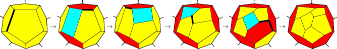
Figure 24: Geometrical construction of a $5$-belt of hexagons

The polytopes $D_{k}$ for $k\geqslant 1$ are exatly nanotubes of type $(5,0)$ [32, 29, 30].

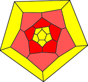
Figure 25: Fullerenes $D_{1}$ and $D_{2}$

Lemma 3.23.

Let $P$ be a flag $3$-polytope without $4$-belts, and let a $5$-loop$\mathcal{L}_{1}=(F_{i_{1}},F_{i_{2}},F_{i_{3}},F_{i_{4}},F_{i_{5}})$ border an $l_{2}$-loop $\mathcal{L}_{2}$, $l_{2}\geqslant 2$, where index $j$ of $i_{j}$ lies in $\mathbb{Z}_{5}=\mathbb{Z}/(5)$. Then one of the following holds:

1. $\mathcal{L}_{1}$ is a $5$-belt (Fig. 26a);

2. $\mathcal{L}_{1}$ is a simple loop consisting of facets surrounding two adjacent edges(Fig. 26b), and $l_{2}=m_{i_{1}}+m_{i_{2}}+m_{i_{3}}+m_{i_{4}}+m_{i_{5}}-19\geqslant 6$;

3. $\mathcal{L}_{1}$ is not a simple loop: $F_{i_{j}}=F_{i_{j+2}}$ for some $j$, $F_{i_{j-2}}\cap F_{i_{j-1}}\cap F_{i_{j}}$ is a vertex, $F_{i_{j+1}}$ does not intersect $F_{i_{j-2}}$ and $F_{i_{j-1}}$ (Fig. 26c), and
   $l_{2}=m_{i_{j-2}}+m_{i_{j-1}}+m_{i_{j}}+m_{i_{j+1}}-13\geqslant 7$.

Figure 26: Possibilities for a $5$-loop $\mathcal{L}_{1}$

Proof 3.24.

Let $\mathcal{L}_{1}$ be not a $5$-belt. If $\mathcal{L}_{1}$ is simple, then two non-successive facets $F_{i_{j}}$ and $F_{i_{j+2}}$ intersect. Then $F_{i_{j}}\cap F_{i_{j+1}}\cap F_{i_{j+2}}$ is a vertex. By Theorem 3.19 the $4$-loop $(F_{i_{j-2}},F_{i_{j-1}},F_{i_{j}},F_{i_{j+2}})$ is not a $4$-belt; hence either $F_{i_{j-2}}\cap F_{i_{j}}\neq\varnothing$, or $F_{i_{j-1}}\cap F_{i_{j+2}}\neq\varnothing$. Up to relabeling in the inverse order, we can assume that $F_{i_{j-1}}\cap F_{i_{j+2}}\neq\varnothing$. Then $F_{i_{j-1}}\cap F_{i_{j}}\cap F_{i_{j+2}}$ and $F_{i_{j-2}}\cap F_{i_{j-1}}\cap F_{i_{j+2}}$ are vertices. Thus $\mathcal{L}_{1}$ surrounds the adjacent edges $F_{i_{j-1}}\cap F_{i_{j+2}}$ and $F_{i_{j}}\cap F_{i_{j+2}}$. By Lemma 3.7 we have $l_{2}=(m_{i_{j-2}}-2)+(m_{i_{j-1}}-3)+(m_{i_{j}}-3)+(m_{i_{j+1}}-2)+(m_{i_{j+2}}-4)-5=m_{i_{1}}+m_{i_{2}}+m_{i_{3}}+m_{i_{4}}+m_{i_{5}}-19\geqslant 6$. The last inequality holds, since flag $3$-polytope without $4$-belts has no triangles and quadrangles. If $\mathcal{L}_{1}$ is not simple, then $F_{i_{j}}=F_{i_{j+2}}$ for some $j$. The successive facets of $\mathcal{L}_{1}$ are different by definition. Let $\mathcal{L}_{1}$ and $\mathcal{L}_{2}$ border the edge cycle $\gamma$ and $\mathcal{L}_{1}\subset\mathcal{D}_{\alpha}$ in notations of Theorem 2.10. Since $F_{i_{j}}$ intersects $\gamma$ by two paths, ${\rm int}\,F_{i_{j-2}}\cup{\rm int}\,F_{i_{j-1}}$ and ${\rm int}\,F_{i_{j+1}}$ lie in different connected components of $\mathcal{C}_{\alpha}\setminus{\rm int}\,F_{i_{j}}$; hence $F_{i_{j-2}}\cap F_{i_{j+1}}=\varnothing=F_{i_{j-1}}\cap F_{i_{j+1}}$. Since $P$ is flag, $F_{i_{j-2}}\cap F_{i_{j-1}}\cap F_{i_{j}}$ is a vertex, thus we obtain the configuration on Fig. 26c. By Lemma 3.7 we have $l_{2}=(m_{i_{j-2}}-2)+(m_{i_{j-1}}-2)+(m_{i_{j}}-3)+(m_{i_{j+1}}-1)-5=m_{i_{j-2}}+m_{j_{j-1}}+m_{i_{j}}+m_{i_{j+1}}-13\geqslant 7$.

The next result follows directly from [29] or [32]. We develop the approach from [10] based on the notion of a $k$-belt.

Theorem 3.25.

Let $P$ be a fullerene. Then the following statements hold.
I. Any pentagonal facet is surrounded by a $5$-belt. There are $12$ belts of this type.
II. If there is a $5$-belt not surrounding a pentagon, then

1. it consists only of hexagons;

2. the fullerene is combinatorially equivalent to the polytope $D_{k}$, $k\geqslant 1$.

3. the number of $5$-belts is $12+k$.

Proof 3.26.

(1) Follows from Proposition 2.5 and Corollary 3.15.

(2) Let the $5$-belt $\mathcal{B}_{5}$ do not surround a pentagon. By Lemma 3.10 it borders an $l_{1}$-loop $\mathcal{L}_{1}\subset\mathcal{W}_{1}$ and an $l_{2}$-loop $\mathcal{L}_{2}\subset\mathcal{W}_{2}$, $l_{1},l_{2}\geqslant 2$, $l_{1}+l_{2}\leqslant 10$. By Lemma 3.12 (1) we have $l_{1},l_{2}\geqslant 3$. From Corollary 3.15 and Lemma 3.12 (2) we obtain $l_{1},l_{2}\geqslant 4$. From Corollary 3.21 and Lemma 3.17 we obtain $l_{1},l_{2}\geqslant 5$. Then $l_{1}=l_{2}=5$ and all facets in $\mathcal{B}_{5}$ are hexagons by Lemma 3.10 (3d). From Lemma 3.23 we obtain that $\mathcal{L}_{1}$ and $\mathcal{L}_{2}$ are $5$-belts. Moving inside $\mathcal{W}_{1}$ we obtain a series of hexagonal $5$-belts, and this series can stop only if the last $5$-belt $\mathcal{B}_{l}$ surrounds a pentagon. Since $\mathcal{B}_{l}$ borders a $5$-belt, Lemma 3.10 (2) implies that $\mathcal{B}_{l}$ consists of pentagons, which have $(2,2,2,2,2)$ edges on the common boundary with a $5$-belt. We obtain the fragment on Fig. 23a). Moving from this fragment backward we obtain a series of hexagonal $5$-belts including $\mathcal{B}_{5}$ with facets having $(2,2,2,2,2)$ edges on both boundaries. This series can finish only with fragment on Fig. 23a) again. Thus any belt not surrounding a pentagon belongs to this series and the number of $5$-belts is equal to $12+k$.

Theorem 3.27.

A fullerene $P$ is combinatorially equivalent to a polytope $D_{k}$ for some $k\geqslant 0$ if and only if it contains the fragment on Fig. 23a).

Proof 3.28.

By Proposition 2.5 the outer $5$-loop of the fragment on Fig. 23a) is a $5$-belt. By the outer boundary component it borders a $5$-loop $\mathcal{L}$. By Lemma 3.23 it is a $5$-belt. If this belt surrounds a pentagon, then we obtain a combinatorial dodecahedron (case $k=0$). If not, then $P$ is combinatorially equivalent to $D_{k}$, $k\geqslant 1$, by Theorem 3.25.

Corollary 3.29.

Any simple $5$-loop of a fullerene

1. either surrounds a pentagon;

2. or is a hexagonal $5$-belt of a fullerene $D_{k}$, $k\geqslant 1$;

3. or surrounds a pair of adjacent edges (Fig. 26b).

Proof 3.30.

Let $\mathcal{L}=(F_{i_{1}},F_{i_{2}},F_{i_{3}},F_{i_{4}},F_{i_{5}})$ be a simple $5$-loop, where index $j$ of $i_{j}$ lies in $\mathbb{Z}_{5}=\mathbb{Z}/(5)$. If $\mathcal{L}$ is a $5$-belt, then by Theorem 3.25, we obtain cases (1) or (2). Otherwise some non-successive facets intersect: $F_{i_{j}}\cap F_{i_{j+2}}\neq\varnothing$ for some $j$. Then $F_{i_{j}}\cap F_{i_{j+1}}\cap F_{i_{j+2}}$ is a vertex. Since a fullerene has no $4$-belts in a simple $4$-loop $(F_{i_{j-2}},F_{i_{j-1}},F_{i_{j}},F_{i_{j+2}})$ either $F_{i_{j-2}}\cap F_{i_{j}}\neq\varnothing$, or $F_{i_{j-1}}\cap F_{i_{j+2}}\neq\varnothing$. Up to relabeling in the inverse order, we can assume that $F_{i_{j-1}}\cap F_{i_{j+2}}\neq\varnothing$. Then $F_{i_{j-1}}\cap F_{i_{j}}\cap F_{i_{j+2}}$ and $F_{i_{j-2}}\cap F_{i_{j-1}}\cap F_{i_{j+2}}$ are vertices. Thus $\mathcal{L}_{1}$ surrounds the adjacent edges $F_{i_{j-1}}\cap F_{i_{j+2}}$ and $F_{i_{j}}\cap F_{i_{j+2}}$.

4 Lecture 4. Moment-angle complexes and moment-angle manifolds

We discuss main notions, constructions and results of toric topology. Details can be found in the monograph [7], which we will follow.

1 Toric topology

Nowadays toric topology is a large research area. Below we discuss applications of toric topology to the mathematical theory of fullerenes based on the following correspondence.

Canonical correspondence
Simple polytope $P$		moment-angle manifold $\mathcal{Z}_{P}$
number of facets $=m$	$\longrightarrow$	canonical $T^{m}$-action on $\mathcal{Z}_{P}$
$\dim P=n$		$\dim\mathcal{Z}_{P}=m+n$
Characteristic function		Quasitoric manifold
$\{F_{1},\dots,F_{m}\}\to\mathbb{Z}^{n}$	$\longrightarrow$	$M^{2n}=\mathcal{Z}_{P}/T^{m-n}$

Algebraic-topological invariants of moment-angle manifolds $\mathcal{Z}_{P}$ give combinatorial invariants of polytopes $P$. As an application we obtain combinatorial invariants of mathematical fullerenes.

2 Moment-angle complex of a simple polytope

Set

$$D^{2}=\{z\in\mathbb{C};|z|\leq 1\},\qquad S^{1}=\{z\in D^{2},|z|=1\}.$$

The multiplication of complex numbers gives the canonical action of the circle $S^{1}$ on the disk $D^{2}$ which orbit space is the interval $\mathbb{I}=[0,1]$.

We have the canonical projection

$$\pi:(D^{2},S^{1})\rightarrow(\mathbb{I},1):z\rightarrow|z|^{2}.$$

By definition a multigraded polydisk is $\mathbb{D}^{2m}=D^{2}_{1}\times\ldots\times D^{2}_{m}$.

Define the standard torus $\mathbb{T}^{m}=S^{1}_{1}\times\ldots\times S^{1}_{m}$.

Proposition 4.1.

There is a canonical action of the torus $\mathbb{T}^{m}$ on the polydisk $\mathbb{D}^{2m}$ with the orbit space

$$\mathbb{D}^{2m}/\mathbb{T}^{m}\simeq\mathbb{I}^{m}=\mathbb{I}^{1}_{1}\times\ldots\times\mathbb{I}^{1}_{m}.$$

Consider a simple polytope $P$. Let $\{F_{1},\dots,F_{m}\}$ be the set of facets and $\{v_{1},\dots,v_{f_{0}}\}$ – the set of vertices. We have the face lattice $L(P)$ of $P$.

Construction (moment-angle complex of a simple polytope [11, 7]): For $P={\rm pt}$ set $\mathcal{Z}_{P}={\rm pt}=\{0\}=\mathbb{D}^{0}$. Let $\dim P>0$. For any face $F\in L(P)$ set

$$\mathcal{Z}_{P,F}=\{(z_{1},\dots,z_{m})\in\mathbb{D}^{2m}\colon z_{i}\in D^{2}_{i}\text{ if }F\subset F_{i},z_{i}\in S^{1}_{i}\text{ if }F\not\subset F_{i}\};$$

$$\mathbb{I}_{P,F}=\{(y_{1},\dots,y_{m})\in\mathbb{I}^{m}\colon y_{i}\in\mathbb{I}^{1}_{i}\text{ if }F\subset F_{i},y_{i}=1\text{ if }F\not\subset F_{i}\}.$$

Proposition 4.2.

1. $\mathcal{Z}_{P,F}\simeq\mathbb{D}^{2k}\times\mathbb{T}^{m-k}$, $\mathbb{I}_{P,F}\simeq\mathbb{I}^{k}$, where $k=n-\dim F$.

2. $\mathcal{Z}_{P,P}=\mathbb{T}^{m}$, $\mathcal{Z}_{P,\varnothing}=\mathbb{D}^{2m}$.

3. If $G_{1}\subset G_{2}$, then $\mathcal{Z}_{P,G_{2}}\subset\mathcal{Z}_{P,G_{1}}$, and $\mathbb{I}_{P,G_{2}}\subset\mathbb{I}_{P,G_{1}}$.

4. $\mathcal{Z}_{P,F}$ is invariant under the action of $\mathbb{T}^{m}$, and the mapping $\pi^{m}\colon\mathbb{D}^{2m}\to\mathbb{I}^{m}$ defines the homeomorphism $\mathcal{Z}_{P,F}/\mathbb{T}^{m}\simeq\mathbb{I}_{P,F}$.

The moment-angle complex of a simple polytope $P$ is a subset in $\mathbb{D}^{2m}$ of the form

$$\mathcal{Z}_{P}=\bigcup_{F\in L(P)\setminus\{\varnothing\}}\mathcal{Z}_{P,F}=\bigcup_{v-\text{ vertex}}\mathcal{Z}_{P,v}.$$

The cube $\mathbb{I}^{m}$ has the canonical structure of a cubical complex. It is a cellular complex with all cells being cubes with an appropriate boundary condition. The cubical complex of a simple polytope $P$ is a cubical subcomplex in $\mathbb{I}^{m}$ of the form

$$\mathbb{I}_{P}=\bigcup_{F\in L(P)\setminus\{\varnothing\}}\mathbb{I}_{P,F}=\bigcup_{v-\text{ vertex}}\mathbb{I}_{P,v}.$$

From the construction of the space $\mathcal{Z}_{P}$ we obtain.

Proposition 4.3.

1. The subset $\mathcal{Z}_{P}\subset\mathbb{D}^{2m}$ is $\mathbb{T}^{m}$ – invariant; hence there is the canonical action of $\mathbb{T}^{m}$ on $\mathcal{Z}_{P}$.

2. The mapping $\pi^{m}$ defines the homeomorphism $\mathcal{Z}_{P}/\mathbb{T}^{m}\simeq\mathbb{I}_{P}$.

3. For $P_{1}\times P_{2}$ we have $\mathcal{Z}_{P_{1}}\times\mathcal{Z}_{P_{2}}$.

3 Admissible mappings

Definition 4.4.

Let $P_{1}$, $P_{2}$ be two simple polytopes. A mapping of sets of facets $\varphi\colon\mathcal{F}_{P_{1}}\to\mathcal{F}_{P_{2}}$ we call admissible, if $\varphi(F_{i_{1}})\cap\dots\cap\varphi(F_{i_{k}})\neq\varnothing$ for any collection $F_{i_{1}},\dots,F_{i_{k}}\in\mathcal{F}_{P_{1}}$ with $F_{i_{1}}\cap\dots\cap F_{i_{k}}\neq\varnothing$.

Any admissible mapping $\varphi\colon\mathcal{F}_{P_{1}}\to\mathcal{F}_{P_{2}}$ induces the mapping $\varphi\colon L(P_{1})\to L(P_{2})$ by the rule: $\varphi(P_{1})=P_{2}$, $\varphi(F_{i_{1}}\cap\dots\cap F_{i_{k}})=\varphi(F_{i_{1}})\cap\dots\cap\varphi(F_{i_{k}})$. This mapping preserves the inclusion relation.

Proposition 4.5.

Any admissible mapping $\varphi\colon\mathcal{F}_{P_{1}}\to\mathcal{F}_{P_{2}}$ induces the mapping of triples $\colon(\mathbb{D}^{2m_{1}},\mathcal{Z}_{P_{1}},\mathbb{T}^{m_{1}})\to(\mathbb{D}^{2m_{2}},\mathcal{Z}_{P_{2}},\mathbb{T}^{m_{2}})$ and the mapping $\mathbb{I}_{P_{1}}\to\mathbb{I}_{P_{2}}$, which we will denote by the same letter $\widehat{\varphi}$:

$$\widehat{\varphi}(x_{1},\dots,x_{m_{1}})=(y_{1},\dots,y_{m_{2}}),\,y_{j}=\begin{cases}1,&\text{ if }\varphi^{-1}(j)=\varnothing,\\ \prod\limits_{i\in\varphi^{-1}(j)}x_{i},&\text{else}.\end{cases}$$

In particular, we have the homomorphism of tori $\mathbb{T}^{m_{1}}\to\mathbb{T}^{m_{2}}$ such that the mapping $\mathcal{Z}_{P_{1}}\to\mathcal{Z}_{P_{2}}$ is equivariant.

We have the commutative diagram

$$\begin{CD}\mathcal{Z}_{P_{1}}@>{\widehat{\varphi}}>{}>\mathcal{Z}_{P_{2}}\\ @V{}V{\pi^{m}}V@V{}V{\pi^{m}}V\\ \mathbb{I}_{P_{1}}@>{\widehat{\varphi}}>{}>\mathbb{I}_{P_{2}}\end{CD}$$

Example 4.6.

Let $P_{1}=\mathbb{I}^{2}$ and $P_{2}=\mathbb{I}$. Then any admissible mapping$\mathcal{F}_{P_{1}}\to\mathcal{F}_{P_{2}}$ is a constant mapping. Indeed, there are two facets $G_{1}$ and $G_{2}$ in $\mathbb{I}$, which do not intersect. $\mathbb{I}^{2}$ has four facets $F_{1},F_{2},F_{3},F_{4}$, such that $F_{1}\cap F_{2}$, $F_{2}\cap F_{3}$, $F_{3}\cap F_{4}$, and $F_{4}\cap F_{1}$ are vertices. Let $\varphi(F_{1})=G_{i}$. Then $\varphi(F_{2})=G_{i}$, since $\varphi(F_{1})\cap\varphi(F_{2})=\varnothing$. By the same reason we have $\varphi(F_{3})=\varphi(F_{4})=G_{i}$. Without loss of generality let $i=1$ and $G_{1}=\{0\}$. Then the mapping of the moment-angle complexes

$$\mathcal{Z}_{\mathbb{I}^{2}}=\{(z_{1},z_{2},z_{3},z_{4})\in\mathbb{D}^{8}\colon|z_{1}|=1\text{ or }|z_{3}|=1,\text{ and }|z_{2}|=1\text{ or }|z_{4}|=1\}=$$

$$=(S^{1}_{1}\times D^{2}_{3}\cup D^{2}_{1}\times S^{1}_{3})\times(S^{1}_{2}\times D^{2}_{4}\cup D^{2}_{2}\times S^{1}_{4})\cong S^{3}\times S^{3},$$

$$\mathcal{Z}_{I^{1}}=\{(w_{1},w_{2})\in\mathbb{D}^{4}\colon|w_{1}|=1\text{ or }|w_{2}|=1\}=$$

$$=(S^{1}_{1}\times D^{2}_{2})\cup(D^{2}_{1}\times S^{1}_{2})\cong S^{3}$$

is

$$\widehat{\varphi}\colon\mathcal{Z}_{\mathbb{I}^{2}}\to\mathcal{Z}_{\mathbb{I}^{1}},\qquad\widehat{\varphi}(z_{1},z_{2},z_{3},z_{4})=(z_{1}z_{2}z_{3}z_{4},1).$$

Example 4.7.

Let $P_{1}=\mathbb{I}^{2}$, $P_{2}=\Delta^{2}$. Then any mapping $\varphi\colon\mathcal{F}_{P_{1}}\to\mathcal{F}_{P_{2}}$ is admissible. Let $\mathcal{F}_{P_{1}}=\{F_{1},F_{2},F_{3},F_{3}\}$ as in previous example, and
$\mathcal{F}_{P_{2}}=\{G_{1},G_{2},G_{3}\}$. The admissible mapping

$$\varphi(F_{1})=G_{1},\quad\varphi(F_{2})=G_{2},\quad\varphi(F_{3})=\varphi(F_{4})=G_{3}$$

induces the mapping of face lattices

$$\varphi(\mathbb{I}^{2})=\Delta^{2},\quad\varphi(\varnothing)=\varnothing,$$

$$\varphi(F_{1}\cap F_{2})=G_{1}\cap G_{2},\quad\varphi(F_{2}\cap F_{3})=G_{2}\cap G_{3},$$

$$\varphi(F_{3}\cap F_{4})=G_{3},\quad\varphi(F_{4}\cap F_{1})=G_{3}\cap G_{1}.$$

The mapping of the moment-angle complexes

$$\mathcal{Z}_{\mathbb{I}^{2}}=\{(z_{1},z_{2},z_{3},z_{4})\in\mathbb{D}^{8}\colon|z_{1}|=1\text{ or }|z_{3}|=1,\text{ and }|z_{2}|=1\text{ or }|z_{4}|=1\}=$$

$$=(S^{1}_{1}\times D^{2}_{3}\cup D^{2}_{1}\times S^{1}_{3})\times(S^{1}_{2}\times D^{2}_{4}\cup D^{2}_{2}\times S^{1}_{4})\cong S^{3}\times S^{3},$$

$$\mathcal{Z}_{\Delta^{2}}=\{(w_{1},w_{2},w_{3})\in\mathbb{D}^{6}\colon|w_{1}|=1,\text{ or }|w_{2}|=1,\text{ or }|w_{3}|=1\}=$$

$$=(S^{1}_{1}\times D^{2}_{2}\times D^{2}_{3})\cup(D^{2}_{1}\times S^{1}_{2}\times D^{2}_{3})\cup(D^{2}_{1}\times D^{2}_{2}\times S^{1}_{3})\cong S^{5}$$

is

$$\widehat{\varphi}\colon\mathcal{Z}_{\mathbb{I}^{2}}\to\mathcal{Z}_{\Delta^{2}},\qquad\varphi(z_{1},z_{2},z_{3},z_{4})=(z_{1},z_{2},z_{3}\cdot z_{4}).$$

4 Barycentric embedding and cubical subdivision of a simple polytope

Construction (barycentric embedding of a simple polytope): Let $P$ be a simple $n$-polytope with facets $F_{1},\dots,F_{m}$. For each face $G\subset P$ define a point $\boldsymbol{x}_{G}$ as a barycenter of it’s vertices. We have $\boldsymbol{x}_{G}\in{\rm relint\,}G$. The points $\boldsymbol{x}_{G}$, $G\in L(P)\setminus\{\varnothing\}$, define a barycentric simplicial subdivision $\Delta(P)$ of the polytope $P$. The simplices of $\Delta(P)$ correspond to flags of faces $F^{a_{1}}\subset F^{a_{2}}\subset\dots\subset F^{a_{k}}$, $\dim F^{i}=i$:

$$\Delta_{F^{a_{1}}\subset F^{a_{2}}\subset\dots\subset F^{a_{k}}}={\rm conv}\{\boldsymbol{x}_{F^{a_{1}}},\boldsymbol{x}_{F^{a_{2}}},\dots,\boldsymbol{x}_{F^{a_{k}}}\},$$

The maximal simplices are $\Delta_{\boldsymbol{v}\subset F^{1}\subset F^{2}\subset\dots\subset F^{n-1}\subset P}$, where $\boldsymbol{v}$ is a vertex. For any point $\boldsymbol{x}\in P$ the minimal simplex $\Delta(\boldsymbol{x})$ containing $\boldsymbol{x}$ can be found by the following rule. Let $G(\boldsymbol{x})=\bigcap\limits_{F_{i}\ni\boldsymbol{x}}F_{i}$. If $\boldsymbol{x}=\boldsymbol{x}_{G}$, then $\Delta(\boldsymbol{x})=\Delta_{G}$. Else take a ray starting in $\boldsymbol{x}_{G}$, passing through $\boldsymbol{x}$ and intersecting $\partial G$ in $\boldsymbol{x}_{1}$. Iterating the argument we obtain either $\boldsymbol{x}_{1}=\boldsymbol{x}_{G_{1}}$, and $\Delta(\boldsymbol{x})=\Delta_{G_{1}\subset G}$, or a new point $\boldsymbol{x}_{2}$. In the end we will stop when $\boldsymbol{x}_{l}=\boldsymbol{x}_{G_{l}}$, and $\Delta(\boldsymbol{x})=\Delta_{G_{l}\subset\dots\subset G_{1}\subset G}$.

Define a piecewise-linear mapping $b_{P}\colon P\to\mathbb{I}^{m}$ by the rule

$$\boldsymbol{x}_{G}\to\widehat{\varepsilon}(G)=(\varepsilon_{1},\dots,\varepsilon_{m})\in\mathbb{I}^{m},\text{where }\varepsilon_{i}=\begin{cases}0,&\text{if }G\subset F_{i},\\ 1,&\text{if }G\not\subset F_{i}\end{cases},$$

on the vertices of $\Delta(P)$, and for any simplex continue the mapping to the cube $\mathbb{I}^{m}$ via barycentric coordinates. In particular, $b_{P}(\boldsymbol{x}_{P})=(1,1,\dots,1)$, and $b_{P}(\boldsymbol{x}_{\boldsymbol{v}})$ is a point with $n$ zero coordinates.

Theorem 4.8.

The mapping $b_{P}$ defines a homeomorphism $P\simeq\mathbb{I}_{P}\subset\mathbb{I}^{m}$.

Proof 4.9.

Let $\boldsymbol{x}\in P$, and $\Delta(\boldsymbol{x})=\Delta_{G_{1}\subset\dots\subset G_{r}}$.

We have $\boldsymbol{x}=t_{1}\boldsymbol{x}_{G_{1}}+\dots+t_{r}\boldsymbol{x}_{G_{r}}$, where $t_{i}>0$, and $t_{1}+\dots+t_{r}=1$. The coordinates of the vector $b_{P}(\boldsymbol{x})=t_{1}\widehat{\varepsilon}(G_{1})+\dots+t_{r}\widehat{\varepsilon}(G_{r})=(x_{1},\dots,x_{m})$ belong to the interval $[0,1]$. Arrange them ascending:

$$0=x_{i_{1}}=\dots=x_{i_{p_{1}}}<x_{i_{p_{1}+1}}=\dots=x_{i_{p_{1}+p_{2}}}<\dots<\\ <x_{i_{p_{1}+\dots+p_{r}+1}}=\dots=x_{i_{m}}=1.$$

Then

$$G_{1}=F_{i_{1}}\cap\dots\cap F_{i_{p_{1}+\dots+p_{r}}},G_{2}=F_{i_{1}}\cap\dots\cap F_{i_{p_{1}+\dots+p_{r-1}}},\dots,G_{r}=F_{i_{1}}\cap\dots\cap F_{i_{p_{1}}},$$

and

$$t_{1}=1-x_{i_{p_{1}+\dots+p_{r}}},t_{2}=x_{i_{p_{1}+\dots+p_{r}}}-x_{i_{p_{1}+\dots+p_{r-1}}},\dots,t_{r}=x_{i_{p_{1}+p_{2}}}.$$

Thus the mapping $b_{P}$ is an embedding. Since $P$ is compact and $\mathbb{I}^{m}$ is Hausdorff, we have the homeomorphism $P\simeq b_{P}(P)$. In the construction above we have $x_{i_{j}}\neq 1$ only if $F_{i_{j}}\supset G_{1}$; hence $b_{P}(\boldsymbol{x})\in\mathbb{I}_{P,G_{1}}$, and $b_{P}(P)\subset\mathbb{I}_{P}$. On the other hand, the above formulas imply that $\mathbb{I}_{P}\subset b_{P}(P)$. This finishes the proof.

Corollary 4.10.

The homeomorphism $b_{P}\colon P\to\mathbb{I}_{P}\simeq\mathcal{Z}_{P}/\mathbb{T}^{m}$ defines a mapping $\pi_{P}\colon\mathcal{Z}_{P}\to P$ such that the following diagram is commutative:

$$\begin{CD}\mathcal{Z}_{P}@>{}>{}>\mathbb{D}^{2m}\\ @V{}V{\pi_{P}}V@V{}V{}V\\ P@>{b_{P}}>{}>\mathbb{I}^{m}\end{CD}$$

Corollary 4.11.

Any admissible mapping $\varphi\colon\mathcal{F}_{P_{1}}\to\mathcal{F}_{P_{2}}$ induces the mapping of polytopes $\widehat{\varphi}\colon P_{1}\to P_{2}$ such that the following diagram is commutative:

$$\begin{CD}\mathcal{Z}_{P_{1}}@>{\widehat{\varphi}}>{}>\mathcal{Z}_{P_{2}}\\ @V{}V{\pi_{P_{1}}}V@V{}V{\pi_{P_{2}}}V\\ P_{1}@>{\widehat{\varphi}}>{}>P_{2}\end{CD}$$

Construction (canonical section): The mapping

$$s:\mathbb{I}\rightarrow D^{2}:s(y)=\sqrt{y}$$

induces the section $s^{m}\colon\mathbb{I}_{P}\to\mathcal{Z}_{P}$. Together with the homeomorphism $P\simeq\mathbb{I}_{P}$ this gives the canonical section $s_{P}=s^{m}\circ b_{P}:P\rightarrow\mathcal{Z}_{P}$, such that $\pi_{P}\circ s_{P}={\rm id}$.

Construction (cubical subdivision): The space $\mathbb{I}_{P}$ has the canonical partition into cubes $\mathbb{I}_{P,v}$, one for each vertex $v\in P^{n}$. The homeomorphism$\mathbb{I}_{P}={\rm Im\,}b_{P}(P)\simeq P$ gives the cubical subdivision of the polytope $P$.

Example 4.12.

For $P=I$ we have an embedding $I\subset I^{2}$.

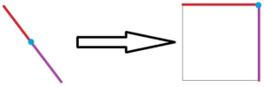
Figure 27: Barycentric embedding and cubical subdivision of the interval

Example 4.13.

For $P=\Delta^{2}$ we have an embedding $\Delta^{2}\subset I^{3}$

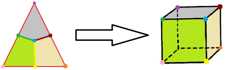
Figure 28: Barycentric embedding and cubical subdivision of the triangle

Construction (product over space): Let $f\colon X\to Z$ and $g\colon Y\to Z$ be maps of topological spaces. The product $X\times_{Z}Y$ over space $Z$ is described by the general pullback diagram:

$$\begin{CD}X\times_{Z}Y@ >>>X\\ @ VVV@ VVfV\\ Y@ >g>>Z\end{CD}$$

where $X\times_{Z}Y=\big{\{}(x,y)\in X\times Y\;:\;f(x)=g(y)\big{\}}$.

Proposition 4.14.

We have $\mathcal{Z}_{P}=\mathbb{D}^{2m}\times_{\mathbb{I}^{m}}P$.

5 Pair of spaces in the power of a simple polytope

Construction (raising to the power of a simple polytope): Let $P$ be a simple polytope $P$ with the face lattice $L(P)$ and the set of facets $\{F_{1},\dots,F_{m}\}$. For $m$ pairs of topological spaces $\{(X_{i},W_{i}),i=1,\dots,m\}$ set $(\boldsymbol{X},\boldsymbol{W})=\{(X_{i},W_{i}),i=1,\dots,m\}$. For a face $F\in L(P)\setminus\{\varnothing\}$ define

$$(\boldsymbol{X},\boldsymbol{W})^{P}_{F}=\{(y_{1},\dots,y_{m})\in X_{1}\times\dots\times X_{m}\colon y_{i}\in X_{i}\text{ if }F\in F_{i},y_{i}\in W_{i}\text{ if }F\notin F_{i}\}.$$

The set of pairs $(\boldsymbol{X},\boldsymbol{W})$ in degree of a simple polytope $P$ is

$$(\boldsymbol{X},\boldsymbol{W})^{P}=\bigcup_{F\in L(P)\setminus\{\varnothing\}}(\boldsymbol{X},\boldsymbol{W})^{P}_{F}$$

Example 4.15.

1. Let $W_{i}=X_{i}$ for all $i$. Then $(\boldsymbol{X},\boldsymbol{W})^{P}=X_{1}\times\dots\times X_{m}$ for any $P$.

2. Let $W_{i}=*_{i}$ – a fixed point in $X_{i}$, $i=1,2$, and $P=I$. Then $(\boldsymbol{X},\boldsymbol{W})^{I}=X_{1}\vee X_{2}$ is the wedge of the spaces $X_{1}$ and $X_{2}$.

Construction (pair of spaces in the power of a simple polytope): In the case $W_{i}=W$, $X_{i}=X$, $i=1,\dots,m$, the space $(\boldsymbol{X},\boldsymbol{W})^{P}$ is called a pair of spaces $(X,W)$ in the power of a simple polytope $P$ and is denoted by $(X,W)^{P}$.

Example 4.16.

The space $(D^{2},S^{1})^{P}$ is the moment-angle complex $\mathcal{Z}_{P}$ of the polytope $P$ (see Subsection 2).

Example 4.17.

The space $(\mathbb{I},1)^{P}$ is the image $\mathbb{I}_{P}=b_{P}(P)$ of the barycentric embedding of the polytope $P$ (see Subsection 2).

Exercise: Describe the space $(X,W)^{P}$, where $P$ is a $5$-gon.

Let us formulate properties of the construction. The proof we leave as an exercise.

Proposition 4.18.

1. Let $P_{1}$ and $P_{2}$ be simple polytopes. Then

   $$(X,W)^{{P_{1}\times P_{2}}}=(X,W)^{P_{1}}\times(X,W)^{P_{2}}$$

2. Let $\{v_{1},\dots,v_{f_{0}}\}$ be the set of vertices of $P$. There is a homeomorphism

   $$(X,W)^{P}\cong\bigcup_{k=1}^{f_{0}}(X,W)^{P}_{v_{k}}$$

3. Any mapping $f\colon(X_{1},W_{1})\to(X_{2},W_{2})$ gives the commutative diagram

   $$\begin{CD}(X_{1},W_{1})^{P}@>{f^{P}}>{}>(X_{2},W_{2})^{P}\\ @V{\cap}V{}V@V{}V{\cap}V\\ (X_{1},X_{1})^{P}=X_{1}^{m}@>{f^{m}}>{}>X_{2}^{m}=(X_{2},X_{2})^{P}\end{CD}$$

4. We have $id^{P}=id$.
   For $f_{1}\colon(X_{1},W_{1})\to(X_{2},W_{2})$, $f_{2}\colon(X_{2},W_{2})\to(X_{1},W_{1})$ we have

   $$(f_{2}\circ f_{1})^{P}=f_{2}^{P}\circ f_{1}^{P}.$$

6 Davis-Januszkiewicz’ construction

Davis-Januszkiewicz’ construction [15]: For $\boldsymbol{x}\in P$ we have the face$G(x)=\bigcap\limits_{F_{i}\supset\boldsymbol{x}}F_{i}\in L(P)$. For a face $G\in L(P)$ define the subgroup $\mathbb{T}^{G}\subset\mathbb{T}^{m}$ as

$$\mathbb{T}^{G}=(S^{1},1)_{G}^{P}=\{(t_{1},\dots,t_{m})\in\mathbb{T}^{m}\colon t_{j}=1,\text{ if }F_{j}\not\ni G\}$$

Set

$$\widetilde{\mathcal{Z}_{P}}=P\times\mathbb{T}^{m}/\sim,$$

where $(\boldsymbol{x}_{1},\boldsymbol{t}_{1})\sim(\boldsymbol{x}_{2},\boldsymbol{t}_{2})\Leftrightarrow\boldsymbol{x}_{1}=\boldsymbol{x}_{2}=\boldsymbol{x}$, and $\boldsymbol{t}_{1}\boldsymbol{t}_{2}^{-1}\in T^{G(\boldsymbol{x})}$.

There is a canonical action of $\mathbb{T}^{m}$ on $\widetilde{\mathcal{Z}_{P}}$ induced by the action of $\mathbb{T}^{m}$ on the second factor.

Theorem 4.19.

The canonical section $s_{P}\colon P\to\mathcal{Z}_{P}$ induces the $\mathbb{T}^{m}$-equivariant homeomorphism

$$\widetilde{\mathcal{Z}_{P}}\longrightarrow\mathcal{Z}_{P}$$

defined by the formula $(\boldsymbol{x},\boldsymbol{t})\to\boldsymbol{t}s_{P}(\boldsymbol{x})$.

7 Moment-angle manifold of a simple polytope

Construction (moment-angle manifold of a simple polytope [12, 7]): Take a simple polytope

$$P=\{\boldsymbol{x}\in\mathbb{R}^{n}\colon\boldsymbol{a}_{i}\boldsymbol{x}+b_{i}\geqslant 0,i=1,\dots,m\}.$$

We have ${\rm rank\,}A=n$, where $A$ is the $m\times n$-matrix with rows $\boldsymbol{a}_{i}$. Then there is an embedding

$$j_{P}\colon P\longrightarrow\mathbb{R}^{m}_{\geq}\,:\,j_{P}(\boldsymbol{x})=(y_{1},\ldots,y_{m}),$$

where $y_{i}=\boldsymbol{a}_{i}\boldsymbol{x}+b_{i}$, and we will consider $P$ as the subset in $\mathbb{R}^{m}_{\geqslant}$.
A moment-angle manifold $\widehat{\mathcal{Z}_{P}}$ is the subset in $\mathbb{C}^{m}$ defined as $\rho^{-1}\circ j_{P}(P)$, where $\rho(z_{1},\ldots,z_{m})=\big{(}|z_{1}|^{2},\ldots,|z_{m}|^{2}\big{)}$. The action of $\mathbb{T}^{m}$ on $\mathbb{C}^{m}$ induces the action of $\mathbb{T}^{m}$ on $\widehat{\mathcal{Z}_{P}}$.

For the embeddings $j_{\mathcal{Z}}\colon\widehat{\mathcal{Z}_{P}}\subset\mathbb{C}^{m}$ and $j_{P}\colon P\subset\mathbb{R}^{m}_{\geqslant}$ we have the commutative diagram:

$$\begin{CD}\widehat{\mathcal{Z}_{P}}@ >{j_{\mathcal{Z}}}>>\mathbb{C}^{m}\\ @ V{\rho_{P}}VV@ VV{\rho}V\\ P@>{j_{P}}>{}>\mathbb{R}_{\geqslant}^{m}\end{CD}$$

Proposition 4.20.

We have $\widehat{\mathcal{Z}_{P}}\subset\mathbb{C}^{m}\setminus\{0\}$.

Proof 4.21.

If $0\in\widehat{\mathcal{Z}_{P}}$, then $0=\rho(0)\in j_{P}(P)$. This corresponds to a point $\boldsymbol{x}\in P$ such that $\boldsymbol{a}_{i}\boldsymbol{x}+b_{i}=0$ for all $i$. This is impossible, since any point of a simple $n$-polytope lies in at most $n$ facets.

Definition 4.22.

For the set of vectors $(\boldsymbol{x}_{1},\dots,\boldsymbol{x}_{m})$ spanning $\mathbb{R}^{n}$, the set of vectors $(\boldsymbol{y}_{1},\dots,\boldsymbol{y}_{m})$ spanning $\mathbb{R}^{m-n}$ is called Gale dual, if for the matrices $X$ and $Y$ with column vectors $\boldsymbol{x}_{i}$ and $\boldsymbol{y}_{j}$ we have $XY^{T}=0$.

Take an $((m-n)\times m)$-matrix $C$ such that $CA=0$ and ${\rm rank\,}C=m-n$. Then the vectors $\boldsymbol{a}_{i}$ and the column vectors $\boldsymbol{c}_{i}$ of $C$ are Gale dual to each other. Let $\boldsymbol{c}_{i}=(c_{1,i},\dots,c_{m-n,i})$.

Proposition 4.23.

We have

$$\widehat{\mathcal{Z}_{P}}=\{\boldsymbol{z}\in\mathbb{C}^{m}\colon c_{i,1}|z_{1}|^{2}+\dots+c_{i,m}|z_{m}|^{2}=c_{i}\},$$

where $c_{i}=c_{i,1}b_{1}+\dots+c_{i,m}b_{m}$.

Denote $\Phi_{i}(\boldsymbol{z})=c_{i,1}|z_{1}|^{2}+\dots+c_{i,m}|z_{m}|^{2}-c_{i}$. Consider the mapping

$$\Phi:\mathbb{C}^{m}\to\mathbb{R}^{m-n}:\;\Phi(\boldsymbol{z})=(\Phi_{1}(\boldsymbol{z}),\ldots,\Phi_{m-n}(\boldsymbol{z})).$$

It is the $\mathbb{T}^{m}$-equivariant quadratic mapping with respect to the trivial action of $\mathbb{T}^{m}$ on $\mathbb{R}^{m-n}$.

Proposition 4.24.

1. $\widehat{\mathcal{Z}_{P}}$ is a complete intersection of real quadratic hypersurfaces in $\mathbb{R}^{2m}\cong\mathbb{C}^{m}$:

   $$\mathcal{F}_{k}=\{\boldsymbol{z}\in\mathbb{C}^{m}:\Phi_{k}(\boldsymbol{z})=0\},\;k=1,\ldots,m-n.$$

2. There is a canonical trivialisation of the normal bundle of the $\mathbb{T}^{m}$-equivariant embedding $\widehat{\mathcal{Z}_{P}}\subset\mathbb{C}^{m}$, that is $\widehat{\mathcal{Z}_{P}}$ has the canonical structure of a framed manifold.

Proof 4.25.

We have $\widehat{\mathcal{Z}_{P}}=\Phi^{-1}(0)$, where $\Phi\colon\mathbb{R}^{2m}\cong\mathbb{C}^{m}\to\mathbb{R}^{m-n}$. Next step is an exercise.

Exercise: Differential $d\Phi\large|_{y}\colon\mathbb{R}^{2m}\to\mathbb{R}^{m-n}$ is an epimorphism for any point of $y\in\Phi^{-1}(0)$.

Corollary 4.26.

For an appropriate choice of $C$

$$\widehat{\mathcal{Z}_{P}}=\bigcap_{k=1}^{m-n}\mathcal{F}_{k}$$

where any surface $\mathcal{F}_{k}\subset\mathbb{R}^{2m}$ is a $(2m-1)$-dimensional smooth $\mathbb{T}^{m}$-manifold.

Proof 4.27.

We just need to find such $C$ that the vector $Cb$ has all coordinates nonzero. For any $C$ above $Cb$ has a nonzero coordinate since $0\notin\widehat{\mathcal{Z}_{P}}$ by Proposition 4.20. Then we can obtain from it the matrix we need by elementary transformations of rows.

Exercise: Describe the orbit space $\mathcal{F}_{k}/\mathbb{T}^{m}$.

Construction (canonical section): The projection $\rho$ has the canonical section

$$s\colon\mathbb{R}^{m}_{\geqslant}\to\mathbb{C}^{m},\qquad s(x_{1},\dots,x_{m})=(\sqrt{x_{1}},\dots,\sqrt{x_{m}}),$$

which gives a canonical section $\widehat{s_{P}}\colon P\to\widehat{\mathcal{Z}_{P}}$ by the formula $\widehat{s_{P}}=s\circ j_{P}$.

Theorem 4.28.

(Smooth structure on the moment-angle complex, [12]) The section $\widehat{s_{P}}\colon P\to\widehat{\mathcal{Z}_{P}}$ induces the $\mathbb{T}^{m}$-equivariant homeomorphism

$$\widetilde{\mathcal{Z}_{P}}\longrightarrow\widehat{\mathcal{Z}_{P}}$$

defined by the formula $(\boldsymbol{x},\boldsymbol{t})\to\boldsymbol{t}\widehat{s_{P}}(\boldsymbol{x})$.

Together with the $\mathbb{T}^{m}$-equivariant homeomorphism $\widetilde{\mathcal{Z}_{P}}\to\mathcal{Z}_{P}$ this gives a smooth structure on the moment-angle complex $\mathcal{Z}_{P}$.

Thus in what follows we identify $\widehat{\mathcal{Z}_{P}}$ and $\mathcal{Z}_{P}$.

Exercise: Describe the manifold $\mathcal{Z}_{P}$ for $P=\{\boldsymbol{x}\in\mathbb{R}^{2}:A\boldsymbol{x}+b\geqslant 0\}$, where

$$1.\quad A^{\top} =\begin{pmatrix}1&0&-1&1\\ 0&1&0&-1\end{pmatrix}, b^{\top} =(0,0,1,1)$$

$$2.\quad A^{\top} =\begin{pmatrix}1&0&-1&1&-1\\ 0&1&0&-1&-1\end{pmatrix}, b^{\top} =(0,0,1,1,2)$$

Exercise: Let $G\subset P$ be a face of codimension $k$ in a simple $n$-polytope $P$, let $\mathcal{Z}_{P}$ be the corresponding moment-angle manifold with the quotient projection $p\colon\mathcal{Z}_{P}\to P$. Show that $p^{-1}(G)$ is a smooth submanifold of $\mathcal{Z}_{P}$ of codimension $2k$. Furthermore, $p^{-1}(G)$ is diffeomorphic to $\mathcal{Z}_{G}\times T^{\ell}$, where $\mathcal{Z}_{G}$ is the moment-angle manifold corresponding to $G$ and $\ell$ is the number of facets of $P$ not intersecting $G$.

8 Mappings of the moment-angle manifold into spheres

For any set $\omega=\{j_{1},\dots,j_{k}\}\subset\{1,\dots,m\}$ define

$$\mathbb{C}^{m-k}_{\omega}=\{(z_{1},\dots,z_{m})\in\mathbb{C}^{m}\colon z_{j}=0,j\in\omega\};$$

$$S^{2m-2k-1}_{\omega}=\{(z_{1},\dots,z_{m})\in\mathbb{C}^{m}\colon z_{j}=0,j\in\omega,\sum_{j\notin\omega}|z_{j}|^{2}=1\};$$

$$\mathbb{R}^{m-k}_{\omega}=\{(y_{1},\dots,y_{m})\in\mathbb{R}^{m}\colon y_{j}=0,j\in\omega\}.$$

Exercise: For $k\geqslant 1$ the sphere $S^{2k-1}_{[m]\setminus\omega}$ is a deformation retract of$S^{2m-1}\setminus S^{2m-2k-1}_{\omega}$.

Proposition 4.29.

1. The embedding $\mathcal{Z}_{P}\subset\mathbb{C}^{m}$ induces the embedding $\mathcal{Z}_{P}\subset S^{2m-1}$ via projection $\mathbb{C}^{m}\setminus\{0\}\to S^{2m-1}$.

2. For any set $\omega$, $|\omega|=k$, such that $\bigcap\limits_{j\in\omega}F_{j}=\varnothing$ the image of the embedding $\mathcal{Z}_{P}\subset S^{2m-1}$ lies in $S^{2m-1}\setminus S^{2m-2k-1}_{\omega}$; hence the embedding is homotopic to the mapping $\varphi_{\omega}\colon\mathcal{Z}_{P}\to S^{2k-1}_{[m]\setminus\omega}$, induced by the projection $\mathbb{C}^{m}\to\mathbb{C}^{k}_{[m]\setminus\omega}$.

Proof 4.30.

(1) follows from Proposition 4.20.

(2) follows from the fact that if $\bigcap\limits_{j\in\omega}F_{j}=\varnothing$, then there is no $\boldsymbol{x}\in P$ such that $\boldsymbol{a}_{j}\boldsymbol{x}+b_{j}=0$ for all $j\in\omega$.

We have the commutative diagram

$$\begin{CD}\mathcal{Z}_{P}@ >>>\mathbb{C}^{m}\setminus\mathbb{C}^{m-k}_{\omega}@>{\xi_{\omega}}>{}>S^{2k-1}_{[m]\setminus\omega}\subset\mathbb{C}^{k}_{[m]\setminus\omega}\\ @ VVV@ VV{\rho}V@V{}V{}V\\ P@>{A\boldsymbol{x}+b}>{}>\mathbb{R}_{\geqslant}^{m}\setminus\mathbb{R}^{m-k}_{\omega}@>{\pi_{\omega}}>{}>{}\Delta^{k-1}\subset\mathbb{R}^{k}_{\geqslant}\end{CD}$$

where

$$\xi_{\omega}(z_{1},\dots,z_{m})=\frac{\boldsymbol{z}_{\omega}}{|\boldsymbol{z}_{\omega}|},\quad\boldsymbol{z}_{\omega}=(z_{j_{1}},\dots,z_{j_{k}}),\quad|\boldsymbol{z}_{\omega}|=\sqrt{|z_{j_{1}}|^{2}+\dots+|z_{j_{k}}|^{2}}.$$

$$\pi_{\omega}(y_{1},\dots,y_{m})=\frac{\boldsymbol{y}_{\omega}}{d_{\omega}},\quad\boldsymbol{y}_{\omega}=(y_{j_{1}},\dots,y_{j_{k}}),\quad d_{\omega}=|y_{j_{1}}|+\dots+|y_{j_{k}}|.$$

Example 4.31.

For any pair of facets $F_{i},F_{j}$, such that $F_{i}\cap F_{j}=\varnothing$, there is a mapping $\mathcal{Z}_{P}\to S^{3}_{[m]\setminus\{i,j\}}$.

Definition 4.32.

The class $a\in H^{k}(X,\mathbb{Z})$ is called cospherical if there is a mapping $\varphi\colon X\to S^{k}$ such that $\varphi^{*}\left(\left[S^{k}\right]\right)=a$.

Corollary 4.33.

For each $\omega\subset[m]$, $|\omega|=k$, such that $\bigcap\limits_{i\in\omega}F_{i}=\varnothing$ we have the cospherical class $\varphi_{\omega}^{*}\left(\left[S^{2k-1}_{[m]\setminus\omega}\right]\right)$ in $H^{2k-1}(\mathcal{Z}_{P})$.

9 Projective moment-angle manifold

Construction (projective moment-angle manifold): Let $S_{\Delta}^{1}$ be the diagonal subgroup in $\mathbb{T}^{m}$. We have the free action of $S_{\Delta}^{1}$ on $\mathcal{Z}_{P}$ and therefore the smooth manifold

$$\mathcal{P}\mathcal{Z}_{P}=\mathcal{Z}_{P}/S_{\Delta}^{1}$$

is the projective version of the moment-angle manifold $\mathcal{Z}_{P}$.

Definition 4.34.

For actions of the commutative group $G$ on spaces $X$ and $Y$ define:

$$X\times_{G}Y=X\times Y/\left\{gx,gy)\sim(x,y)\,\forall x\in X,y\in Y,g\in G\right\}.$$

Corollary 4.35.

For any simple polytope $P$ there exists the smooth manifold

$$W=\mathcal{Z}_{P}\times_{S_{\Delta}^{1}}D^{2}$$

such that $\partial W=\mathcal{Z}_{P}$.

We have the fibration $W\longrightarrow\mathcal{P}\mathcal{Z}_{P}$ with the fibre $D^{2}$.
Exercise: $P=\Delta^{n}\Longleftrightarrow\mathcal{Z}_{P}=S^{2n+1}\Longrightarrow\mathcal{P}S^{2n+1}=\mathbb{C}P^{n}$.

The constructions of the subsection 8 respect the diagonal action of $S^{1}$; hence we obtain the following results.

For $k\geqslant 1$ the set $\mathbb{C}P^{k-1}_{[m]\setminus\omega}$ is a deformation retract of $\mathbb{C}P^{m-1}\setminus\mathbb{C}P^{m-k-1}_{\omega}$.

Proposition 4.36.

1. The embedding $\mathcal{Z}_{P}\subset\mathbb{C}^{m}$ induces the embedding $\mathcal{P}\mathcal{Z}_{P}\subset\mathbb{C}P^{m-1}$.

2. For any set $\omega$, $|\omega|=k$, such that $\bigcap\limits_{j\in\omega}F_{j}=\varnothing$ the image of the embedding $\mathcal{P}\mathcal{Z}_{P}\subset\mathbb{C}P^{m}$ lies in $\mathbb{C}P^{m-1}\setminus\mathbb{C}P^{m-k-1}_{\omega}$; hence the embedding is homotopic to the mapping $\mathcal{P}\mathcal{Z}_{P}\to\mathbb{C}P^{k-1}_{[m]\setminus\omega}$, induced by the projection $\mathbb{C}^{m}\to\mathbb{C}^{k}_{[m]\setminus\omega}$.

5 Lecture 5. Cohomology of a moment-angle manifold

When we deal with homology and cohomology, if it is not specified, the notation $H^{*}(X)$ and $H_{*}(X)$ means that we consider integer coefficients.

1 Cellular structure

Define a cellular structure on $D^{2}$ consisting of $3$ cells:

$$p=\{1\},\quad U=S^{1}\setminus\{1\},\quad V=D^{2}\setminus S^{1}.$$

Set on $D^{2}$ the standard orientation, with $(1,0)$ and $(0,1)$ being the positively oriented basis, and on $S^{1}$ the counterclockwise orientation induced from $D^{2}$. Then in the chain complex $C_{*}(D^{2})$ we have

$$dp=0,\quad dU=0,\quad dV=U.$$

The coboundary operator $\partial\colon C^{i}(X)\to C^{i+1}(X)$ is defined by the rule $\langle\partial\varphi,a\rangle=\langle\varphi,da\rangle$. For a cell $E$ let us denote by $E^{*}$ the cochain such that $\langle E^{*},E^{\prime}\rangle=\delta(E,E^{\prime})$ for any cell $E^{\prime}$. Denote $p^{*}=1$. Then the coboundary operator in $C^{*}(D^{2})$ has the form

$$\partial 1=0,\quad\partial U^{*}=V^{*},\quad\partial V^{*}=0.$$

By definition the multigraded polydisk $\mathbb{D}^{2m}$ has the canonical multigraded cellular structure , which is a product of cellular structures of disks, with cells corresponding to pairs of sets $\sigma,\omega$, $\sigma\subset\omega\subset[m]=\{1,2,\dots,m\}$.

$$C_{\sigma,\omega}=\tau_{1}\times\dots\times\tau_{m},\tau_{j}=\begin{cases}V_{j},&j\in\sigma,\\ U_{j},&j\in\omega\setminus\sigma,\\ p_{j},&j\in[m]\setminus\omega\end{cases},\;mdeg\,C_{\sigma,\omega}=(-i,2\omega),$$

where $i=|\omega\setminus\sigma|$. Then the cellular chain complex $C_{*}(\mathbb{D}^{2m})$ is the tensor product of $m$ chain complexes $C_{*}(D^{2}_{i})$, $i=1,\dots,m$. The boundary operator $d$ of the chain complex respects the multigraded structure and can be considered as a multigraded operator of $mdeg\;d=(-1,0)$. It can be calculated on the elements of the tensor product by the the Leibnitz rule

$$d(a\times b)=(da)\times b+(-1)^{\dim a}a\times(db).$$

For cochains the $\times$-operation $C^{i}(X)\times C^{j}(Y)\to C^{i+j}(X\times Y)$ is defined by the rule $\langle\varphi\times\psi,a\times b\rangle=\langle\varphi,a\rangle\langle\psi,b\rangle$. Then

$$\langle\psi_{1}\times\dots\times\psi_{m},a_{1}\times\dots\times a_{m}\rangle=\langle\psi_{1},a_{1}\rangle\dots\langle\psi_{m},a_{m}\rangle.$$

The basis in $C^{*}(\mathbb{D}^{2m})$ is formed by the cochains $C^{*}_{\sigma,\omega}=\tau_{1}^{*}\times\dots\times\tau_{m}^{*}$, where $C_{\sigma,\omega}=\tau_{1}\times\dots\times\tau_{m}$.

The coboubdary operator $\partial$ is also multigraded. It has multidegree $mdeg\;\partial=(1,0)$. It can be calculated on the elements of the tensor algebra $C^{*}(\mathbb{D}^{2m})$ by the rule $\partial(\varphi\times\psi)=(\partial\varphi)\times\psi+(-1)^{\dim\varphi}\varphi\times(\partial\psi)$.

Proposition 5.1.

The moment-angle complex $\mathcal{Z}_{P}$ has the canonical structure of a multigraded subcomplex in the multigraded cellular structure of $\mathbb{D}^{2m}$. The projection $\mathbb{\pi}^{m}\colon\mathcal{Z}_{P}\to\mathbb{I}_{P}$ is cellular.

Theorem 5.2.

There is a multigraded structure in the cohomology group:

$$H^{n}(\mathcal{Z}_{P},\mathbb{Z})\simeq\bigoplus\limits_{2|\omega|=n+i}H^{-i,2\omega}(\mathcal{Z}_{P},\mathbb{Z}),$$

where for $\omega=\{j_{1},\dots,j_{k}\}$, we have $|\omega|=k$.

Proof 5.3.

The multigraded structure in cohomology is induced by the multigraded cellular structure described above.

Example 5.4.

Let $P=\Delta^{n}$, then $\mathcal{Z}_{P}=S^{2n+1}$. In the case $n=1$ the simplex $\Delta^{1}$ is an interval $I$, and we have the decomposition $\mathcal{Z}_{I}=S^{3}=S^{1}\times D^{2}\cup D^{2}\times S^{1}$. The space $\mathcal{Z}_{I}$ consists of $8$ cells

$$p_{1}\times p_{2}$$

$$p_{1}\times U_{2},\quad U_{1}\times p_{2}$$

$$p_{1}\times V_{2},\quad U_{1}\times U_{2},\quad V_{1}\times p_{2},$$

$$U_{1}\times V_{2},\quad V_{1}\times U_{2}$$

We have

$$H^{*}(S^{3})=H^{0,2\varnothing}(S^{3})\oplus H^{-1,2\{1,2\}}(S^{3}).$$

2 Multiplication

Now following [7] we will describe the cohomology ring of a moment-angle complex in terms of the cellular structure defined above. This result is non-trivial, since the problem to define the multiplication in cohomology in terms of cellular cochains in general case is unsolvable. The reason is that the diagonal mapping used in the definition of the cohomology product is not cellular, and a cellular approximation can not be made functorial with respect to arbitrary cellular mappings. We construct a canonical cellular diagonal approximation $\widetilde{\Delta}\colon\mathcal{Z}_{P}\to\mathcal{Z}_{P}\times\mathcal{Z}_{P}$, which is functorial with respect to mappings induced by admissible mapping of sets of facets of polytopes.

Remind, that the product in the cohomology of a cell complex $X$ is defined as follows. Consider the composite mapping of cellular cochain complexes

$$\mathcal{C}^{*}(X)\otimes\mathcal{C}^{*}(X)\stackrel{{\scriptstyle\times}}{{\longrightarrow}}\mathcal{C}^{*}(X\times X)\stackrel{{\scriptstyle\widetilde{\Delta}^{*}}}{{\longrightarrow}}\mathcal{C}^{*}(X).$$ (2)

Here the mapping $\times$ sends a cellular cochain $c_{1}\otimes c_{2}\in C^{q_{1}}(X)\otimes C^{q_{2}}(X)$ to the cochain $c_{1}\times c_{2}\in C^{q_{1}+q_{2}}(X\times X)$, whose value on a cell $e_{1}\times e_{2}\in C_{*}(X\times X)$ is $\langle c_{1},e_{1}\rangle\langle c_{2},e_{2}\rangle$. The mapping $\widetilde{\Delta}^{*}$ is induced by a cellular mapping $\widetilde{\Delta}$ (a cellular diagonal approximation) homotopic to the diagonal $\Delta\colon X\to X\times X$. In cohomology, the mapping (2) induces a multiplication $H^{*}(X)\otimes H^{*}(X)\to H^{*}(X)$ which does not depend on the choice of a cellular approximation and is functorial. However, the mapping (2) itself is not functorial because there is no choice of a cellular approximation compatible with arbitrary cellular mappings.

Define polar coordinated in $D^{2}$ by $z=\rho e^{i\varphi}$.

Proposition 5.5.

1. The mapping $\Delta_{t}\colon\mathbb{I}\times D^{2}\to D^{2}\times D^{2}$: $\rho e^{i\varphi}\to$

   $$\to\begin{cases}\left((1-\rho)t+\rho e^{i(1+t)\varphi},(1-\rho)t+\rho e^{i(1-t)\varphi}\right),&\varphi\in[0,\pi],\\ \left((1-\rho)t+\rho e^{i(1-t)\varphi+2\pi it},(1-\rho)t+\rho e^{i(1+t)\varphi-2\pi it}\right),&\varphi\in[\pi,2\pi]\end{cases}$$

   defines the homotopy of mappings of pairs $(D^{2},S^{1})\to(D^{2}\times D^{2},S^{1}\times S^{1})$.

2. The mapping $\Delta_{0}$ is the diagonal mapping $\Delta\colon D^{2}\to D^{2}\times D^{2}$.

3. The mapping $\Delta_{1}$ is

   $$\rho e^{i\varphi}\to\begin{cases}((1-\rho)+\rho e^{2i\varphi},1),&\varphi\in[0,\pi],\\ (1,(1-\rho)+\rho e^{2i\varphi}),&\varphi\in[\pi,2\pi]\end{cases}$$

   It is cellular and sends the pair $(D^{2},S^{1})$ to the pair of wedges
   $(D^{2}\times 1\vee 1\times D^{2},S^{1}\times 1\vee 1\times S^{1})$ in the point $(1,1)$. Hence it is a cellular approximation of $\Delta$.

4. We have

   $$(\Delta_{1})_{*}p=p\times p,\,(\Delta_{1})_{*}U=U\times p+p\times U,\,(\Delta_{1})_{*}V=V\times p+p\times V;$$

   hence

   $$(U^{*})^{2}=\langle U^{*}\times U^{*},(\Delta_{1})_{*}V\rangle V^{*}=\langle U^{*}\times U^{*},V\times p+p\times V\rangle V^{*}=0,$$

   and the multiplication of cochains in $\mathcal{C}^{*}(D^{2})$ induced by $\Delta_{1}$ is trivial:

   $$1\cdot X=X=X\cdot 1,\quad(U^{*})^{2}=U^{*}V^{*}=V^{*}U^{*}=(V^{*})^{2}=0.$$

The proof we leave as an exercise.

Using the properties of the construction of the moment-angle complex we obtain the following result.

Corollary 5.6.

1. For any simple polytope $P$ with $m$ facets there is a homotopy

   $$\Delta_{t}^{m}\colon(\mathbb{D}^{2m},\mathcal{Z}_{P})\to(\mathbb{D}^{2m}\times\mathbb{D}^{2m},\mathcal{Z}_{P}\times\mathcal{Z}_{P}),$$

   where $\Delta_{0}^{m}$ is the diagonal mapping and $\Delta_{1}^{m}$ is a cellular mapping.

2. In the cellular cochain complex of $\mathbb{D}^{2m}=D^{2}\times\dots\times D^{2}$ the multiplication defined by $\Delta_{1}^{m}$ is the tensor product of multiplications of the factors defined by the rule $(\varphi_{1}\times\varphi_{2})(\psi_{1}\times\psi_{2})=(-1)^{\dim\varphi_{2}\dim\psi_{1}}\varphi_{1}\psi_{1}\times\varphi_{2}\psi_{2}$, and

   $$(\varphi_{1}\times\dots\times\varphi_{m})(\psi_{1}\times\dots\times\psi_{m})=(-1)^{\sum\limits_{i>j}\dim\varphi_{i}\dim\psi_{j}}\varphi_{1}\psi_{1}\times\dots\times\varphi_{m}\psi_{m},$$

   and respects the multigrading.

3. The multiplication in $\mathcal{C}^{*}(\mathcal{Z}_{P})$ given by $\Delta^{m}_{1}$ is defined from the inclusion
   $\mathcal{Z}_{P}\subset\mathbb{D}^{2m}$ as a multigraded cellular subcomplex.

3 Description in terms of the Stanley-Reisner ring

Definition 5.7.

Let $\{F_{1},\dots,F_{m}\}$ be the set of facets of a simple polytope $P$. Then a Stanley-Reisner ring of $P$ over $\mathbb{Z}$ is defined as a monomial ring

$$\mathbb{Z}[P]=\mathbb{Z}[v_{1},\dots,v_{m}]/J_{SR}(P),$$

where

$$J_{SR}(P)=(v_{i_{1}}\dots v_{i_{k}},\text{ if }F_{i_{1}}\cap\dots\cap F_{i_{k}}=\varnothing)$$

is the Stanley-Reisner ideal.

Example 5.8.

$\mathbb{Z}[\Delta^{2}]=\mathbb{Z}[v_{1},v_{2},v_{3}]/(v_{1}v_{2}v_{3})$

Theorem 5.9.

(see [4]) Two polytopes are combinatorially equivalent if and only if their Stanley-Reisner rings are isomorphic.

Corollary 5.10.

Fullerenes $P_{1}$ and $P_{2}$ are combinatorially equivalent if and only if there is an isomorphism $\mathbb{Z}[P_{1}]\cong\mathbb{Z}[P_{2}]$.

Theorem 5.11.

The Stanley-Reisner ring of a flag polytope is a monomial quadratic ring:

$$J_{SR}(P)=\{v_{i}v_{j}:F_{i}\cap F_{j}=\varnothing\}.$$

Figure 29: Cube $I^{2}$. We have $J_{SR}(I^{2})=\{v_{1}v_{3},v_{2}v_{4}\}$

Each fullerene is a simple flag polytope (Theorem 3.13).

Corollary 5.12.

The Stanley-Reisner ring of a fullerene is monomial quadratic.

Construction (multigraded complex): For a set $\sigma\subset[m]$ define $G(\sigma)=\bigcap\limits_{i\in\sigma}F_{i}$. Conversely, for a face $G$ define $\sigma(G)=\{i\colon G\subset F_{i}\}\subset[m]$. Then $\sigma(G(\sigma))=\sigma$, and $G(\sigma(G))=G$. Let

$$R^{*}(P)=\Lambda[u_{1},\dots,u_{m}]\otimes\mathbb{Z}[P]/(u_{i}v_{i},v_{i}^{2}),$$

$${\rm mdeg}\;u_{i}=(-1,2\{i\}),{\rm mdeg}\;v_{i}=(0,2\{i\}),du_{i}=v_{i},dv_{i}=0$$

be a multigraded differential algebra. It is additively generated by monomials $v_{\sigma}u_{\omega\setminus\sigma}$, where $v_{\sigma}=\prod\limits_{i\in\sigma}v_{i}$, $G(\sigma)\neq\varnothing$, and $u_{\omega\setminus\sigma}=u_{j_{1}}\wedge\dots\wedge u_{j_{l}}$ for $\omega\setminus\sigma=\{j_{1},\dots,j_{l}\}$.

Theorem 5.13.

[7] We have a mutigraded ring isomorphism

$$H[R^{*}(P),d]\simeq H^{*}(\mathcal{Z}_{P},\mathbb{Z})$$

Proof 5.14.

Define the mapping $\zeta\colon R^{*}(P)\to C^{*}(\mathcal{Z}_{P})$ by the rule $\zeta(v_{\sigma}u_{\omega\setminus\sigma})=C^{*}_{\sigma,\omega}$. It is a graded ring isomorphism from Proposition 5.5(4), and Corollary 5.6. The formula $\zeta(dv_{\sigma}u_{\omega\setminus\sigma})=\partial C^{*}_{\sigma,\omega}$ follows from the Leibnitz rule.

Exercise: Prove that for the cospherical class $\varphi_{\omega}^{*}\left(\left[S^{2k-1}_{[m]\setminus\omega}\right]\right)$, $\omega=\{i_{1},\dots,i_{k}\}$, (see Corollary 4.33) we have $\varphi_{\omega}^{*}\left(\left[S^{2k-1}_{[m]\setminus\omega}\right]\right)=\pm[u_{i_{1}}v_{i_{2}}\dots v_{i_{k}}]\in H[R^{*}(P),d]$.

4 Description in terms of unions of facets

Let $P_{\omega}=\bigcup\limits_{i\in\omega}F_{i}$ for a subset $\omega\subset[m]$. By definition $P_{\varnothing}=\varnothing$, and $P_{[m]}=\partial P$.

Definition 5.15.

For two sets $\sigma,\tau\subset[m]$ define $l(\sigma,\tau)$ to be the number of pairs $\{(i,j)\colon i\in\sigma,j\in\tau,i>j\}$. We write $l(i,\tau)$ and $l(\sigma,j)$ for $\sigma=\{i\}$ and $\tau=\{j\}$ respectively.

Comment: The number $(-1)^{l(\sigma,\omega)}$ is used for definition of the multiplication of cubical chain complexes (see [38]). In the discrete mathematics the number $l(\sigma,\tau)$ is a characteristic of two subsets $\sigma,\tau$ of an ordered set.

Proposition 5.16.

We have

1. $l(\sigma,\tau)=\sum\limits_{i\in\sigma}l(i,\tau)=\sum\limits_{j\in\tau}l(\sigma,j)=\sum\limits_{i\in\sigma,j\in\tau}l(i,j)$.

2. $l(\sigma,\tau_{1}\sqcup\tau_{2})=l(\sigma,\tau_{1})+l(\sigma,\tau_{2})$, $l(\sigma_{1}\sqcup\sigma_{2},\tau)=l(\sigma_{1},\tau)+l(\sigma_{2},\tau)$.

3. $l(\sigma,\tau)+l(\tau,\sigma)=|\sigma||\tau|-|\sigma\cap\tau|$.
   In particular, if $\sigma\cap\tau=\varnothing$, then $l(\sigma,\tau)+l(\tau,\sigma)=|\tau||\sigma|$.

Definition 5.17.

Set

$$\mathbb{I}_{P,\omega}=\bigcup\limits_{G\neq\varnothing\colon\sigma(G)\subset\omega}\mathbb{I}_{P,G}=\{(x_{1},\dots,x_{m})\in\mathbb{I}_{P}\colon x_{i}=1,i\notin\omega\}.$$

Theorem 5.18.

[7] For any $\omega\subset[m]$ there is an isomorphism:

$$H^{-i,2\omega}(\mathcal{Z}_{P},\mathbb{Z})\cong{H}^{|\omega|-i}(P,P_{\omega},\mathbb{Z}),$$

Proof 5.19.

For subsets $A\subset\mathbb{I}^{m}$ and $\omega\subset[m]$ define

$$A^{\omega}=\{(y_{1},\dots,y_{m})\in A\colon y_{i}=0\text{ for some }i\in\omega\},\quad A^{0}=A^{[m]}.$$

We have $A^{\varnothing}=A$. There is a homeomorphism of pairs $(P,P_{\omega})\simeq(\mathbb{I}_{P},\mathbb{I}_{P}^{\omega})$.

The homotopy $r^{\omega}_{t}\colon\mathbb{I}^{m}\to\mathbb{I}^{m}$:

$$r^{\omega}_{t}(y_{1},\dots,y_{m})=(y_{1}^{\prime},\dots,y_{m}^{\prime}),y_{j}^{\prime}=\begin{cases}(1-t)y_{j}+t,&j\notin\omega;\\ y_{j},&j\in\omega,\end{cases}$$

gives a deformation retraction $r^{\omega}=r^{\omega}_{1}\colon(\mathbb{I}_{P},\mathbb{I}_{P}^{\omega})\to(\mathbb{I}_{P,\omega},\mathbb{I}_{P,\omega}^{0})$.

There is a natural multigraded cell structure on the cube $\mathbb{I}^{m}$, induced by the cell structure on $\mathbb{I}$ consisting of $3$ cells: $\mathbf{0}=\{0\}$, $\mathbf{1}=\{1\}$ and $J=(0,1)$. All the sets $\mathbb{I}_{P}$, $\mathbb{I}_{P,G}$, $\mathbb{I}_{P}^{\omega}$, $\mathbb{I}_{P,\omega}$, $\mathbb{I}_{P,\omega}^{0}$ are cellular subcomplexes. There is a natural orientation in $J$ such that $\mathbf{0}$ is the beginning, and $\mathbf{1}$ is the end. We have

$$d\mathbf{0}=d\mathbf{1}=0,\quad dJ=\mathbf{1}-\mathbf{0};$$

$$\partial\mathbf{1}^{*}=-\partial\mathbf{0}^{*}=J^{*},\quad\partial J^{*}=0.$$

The cells in $\mathbb{I}^{m}$ has the form $\eta_{1}\times\dots\times\eta_{m}$, $\eta_{i}\in\{\mathbf{0}_{i},\mathbf{1}_{i},J_{i}\}$. There is natural cellular approximation for the diagonal mapping $\Delta\colon\mathbb{I}\to\mathbb{I}\times\mathbb{I}$ by the mapping $\Delta_{1}$:

$$\Delta_{1}(x)=\begin{cases}(2x,1),&x\in[0,\frac{1}{2}],\\ (1,2x-1),&x\in[\frac{1}{2},1],\end{cases}$$

connected with $\Delta$ by the homotopy $\Delta_{t}=(1-t)\Delta+t\Delta_{1}$. Then

$$(\Delta_{1})_{*}\mathbf{0}=\mathbf{0}\times\mathbf{0},\quad(\Delta_{1})_{*}\mathbf{1}=\mathbf{1}\times\mathbf{1},\quad(\Delta_{1})_{*}J=J\times\mathbf{0}+\mathbf{1}\times J,$$

and for the induced multiplication we have

$$(\mathbf{0}^{*})^{2}=\mathbf{0}^{*},\quad(\mathbf{1}^{*})^{2}=\mathbf{1}^{*},\quad\mathbf{0}^{*}\mathbf{1}^{*}=\mathbf{1}^{*}\mathbf{0}^{*}=0,\quad\mathbf{0}^{*}J^{*}=J^{*}\mathbf{1}^{*}=0,$$

$$J^{*}\mathbf{0}^{*}=\mathbf{1}^{*}J^{*}=J^{*},\quad(J^{*})^{2}=0.$$

The cells in $\mathbb{I}_{P,\omega}\setminus\mathbb{I}_{P,\omega}^{0}$ have the form

$$E_{\sigma}=\eta_{1}\times\dots\times\eta_{m},\quad\eta_{j}=\begin{cases}J_{j},&j\in\sigma,\\ 1,&j\notin\sigma,\end{cases},$$

where $\sigma\subset\omega$, and $G(\sigma)\neq\varnothing$. Then $E^{*}_{\sigma}=\eta_{1}^{*}\times\dots\times\eta_{m}^{*}$.

Now define the mapping $\xi_{\omega}\colon R^{-i,2\omega}\to C^{|\omega|-i}(\mathbb{I}_{P,\omega},\mathbb{I}_{P,\omega}^{0})$ by the rule

$$\xi_{\omega}(u_{\omega\setminus\sigma}v_{\sigma})=(-1)^{l(\sigma,\omega)}E^{*}_{\sigma}.$$

By construction $\xi_{\omega}$ is an additive isomorphism. For $\sigma\subset\omega$ we have

$$\partial\xi_{\omega}(v_{\sigma}u_{\omega\setminus\sigma})=\partial\left((-1)^{l(\sigma,\omega)}E^{*}_{\sigma}\right)=(-1)^{l(\sigma,\omega)}\!\!\!\!\!\!\!\!\!\!\sum\limits_{j\in\omega\setminus\sigma,G(\sigma\sqcup\{j\})\neq\varnothing}(-1)^{l(j,\sigma)}E^{*}_{\sigma\sqcup\{j\}},$$

On the other hand,

$$\xi_{\omega}(dv_{\sigma}u_{\omega\setminus\sigma})=\xi_{\omega}\left(\sum\limits_{j\in\omega\setminus\sigma,G(\sigma\sqcup\{j\})\neq\varnothing}(-1)^{l(j,\omega\setminus\sigma)}v_{\sigma\sqcup\{j\}}u_{\omega\setminus(\sigma\sqcup\{j\})}\right)=\\ =\sum\limits_{j\in\omega\setminus\sigma,G(\sigma\sqcup\{j\})\neq\varnothing}(-1)^{l(\sigma\sqcup\{j\},\omega)}(-1)^{l(j,\omega\setminus\sigma)}E^{*}_{\sigma\sqcup\{j\}}$$

Now the proof follows from the formula

$$l(\sigma\sqcup\{j\},\omega)+l(j,\omega\setminus\sigma)=l(\sigma,\omega)+l(j,\omega)+l(j,\omega\setminus\sigma)=l(\sigma,\omega)+l(j,\sigma)+2l(j,\omega\setminus\sigma)$$

Corollary 5.20.

[7] For any $\omega\subset[m]$ there is an isomorphism:

$$H^{-i,2\omega}(\mathcal{Z}_{P},\mathbb{Z})\cong\widetilde{H}^{|\omega|-i-1}(P_{\omega},\mathbb{Z}),$$

where by definition $\widetilde{H}^{-1}(\varnothing,\mathbb{Z})=\mathbb{Z}$.

The proof follows from the long exact sequence in the reduced cohomology of the pair $(P,P_{\omega})$, since $P$ is contractible.

5 Multigraded Betti numbers and the Poincare duality

Definition 5.21.

Define multigraded Betti numbers $\beta^{-i,2\omega}={\rm rank\,}H^{-i,2\omega}(\mathcal{Z}_{P})$. We have

$$\beta^{-i,2\omega}={\rm rank\,}H^{|\omega|-i}(P,P_{\omega})={\rm rank\,}\widetilde{H}^{|\omega|-i-1}(P_{\omega},\mathbb{Z}).$$

From Proposition 4.24 the manifold $\widehat{\mathcal{Z}_{P}}$ is oriented.

Proposition 5.22.

We have

$$\beta^{-i,2\omega}=\beta^{-(m-n-i),2([m]\backslash\omega)}.$$

Proof 5.23.

From the Poincare duality theorem the bilinear form $H^{*}(\mathcal{Z}_{P})\otimes H^{*}(\mathcal{Z}_{P})\to\mathbb{Z}$ defined by

$$\langle\varphi,\psi\rangle=\langle\varphi\psi,[\mathcal{Z}_{P}]\rangle,$$

where $[\mathcal{Z}_{P}]$ is a fundamental cycle, is non-degenerate if we factor out the torsion. This means that there is a basis for which the matrix of the bilinear form has determinant $\pm 1$. For mutligraded ring this means that the matrix consists of blocks corresponding to the forms

$$H^{-i,2\omega}(\mathcal{Z}_{P})\otimes H^{-(m-n-i),2([m]\backslash\omega)}(\mathcal{Z}_{P})\to\mathbb{Z}.$$

Hence all blocks are squares and have determinant $\pm 1$, which finishes the proof.

Let the polytope $P$ be given in the irredundant form $\{\boldsymbol{x}\in\mathbb{R}^{n}\colon A\boldsymbol{x}+b\geqslant 0\}$. For the vertex $v=F_{i_{1}}\cap\dots\cap F_{i_{n}}$ define the submatrix $A_{v}$ in $A$ corresponding to the rows $i_{1},\dots,i_{n}$.

Proposition 5.24.

The fundamental cycle $[\mathcal{Z}_{P}]$ can be represented by the following element in $C_{-(m-n),[m]}(\mathcal{Z}_{P})$:

$$Z=\sum\limits_{v\text{ -- vertex}}(-1)^{l(\sigma(v),[m])}{\rm sign}(\det A_{v})C_{\sigma(v),[m]}.$$

Then the form

$$C^{-i,\omega}(\mathcal{Z}_{P})\otimes C^{-(m-n-i),[m]\setminus\omega}(\mathcal{Z}_{P})\to\mathbb{Z}$$

is defined by the property

$$\langle u_{[m]\setminus\sigma(v)}v_{\sigma(v)},Z\rangle=(-1)^{l(\sigma(v),m)}{\rm sign}(\det A_{v}).$$

The idea of the proof is to use the Davis–Januszkiewicz’ construction. The space $P^{n}\times\mathbb{T}^{m}$ has the orientation defined by orientations of $P^{n}$ and $S^{1}$. Then the mapping

$$P^{n}\times\mathbb{T}^{m}\to\mathcal{Z}_{P}\colon(\boldsymbol{x},\boldsymbol{t})\to\boldsymbol{t}s_{P}(\boldsymbol{x})$$

defines the orientation of the cells $C_{\sigma(v),[m]}$.

6 Multiplication in terms of unions of facets

For pairs of spaces define the direct product as

$$(X,A)\times(Y,B)=(X\times Y,A\times Y\cup X\times B).$$

There is a canonical multiplication in the cohomology of cellular pairs

$$H^{k}(X,A)\otimes H^{l}(X,B)\to H^{k+l}(X,A\cup B)$$

defined in the cellular cohomology by the rule

$$H^{k}(X,A)\otimes H^{l}(X,B)\xrightarrow{\times}H^{k+l}((X,A)\times(X,B))\xrightarrow{\widetilde{\Delta}^{*}}H^{k+l}(X,A\cup B),$$

where $\widetilde{\Delta}$ is a cellular approximation of the diagonal mapping

$$\Delta\colon(X,A\cup B)\to(X,A)\times(X,B).$$

Thus for any simple polytope $P$ and subsets $\omega_{1},\omega_{2}\subset[m]$, we have the canonical multiplication

$$H^{k}(P,P_{\omega_{1}})\otimes H^{l}(P,P_{\omega_{2}})\to H^{k+l}(P,P_{\omega_{1}\cup\omega_{2}}).$$

Theorem 5.25.

There is the ring isomorphism

$$H^{*}(\mathcal{Z}_{P})\simeq\bigoplus\limits_{\omega\subset[m]}H^{*}(P,P_{\omega})$$

where the multiplication on the right hand side

$$H^{|\omega_{1}|-k}(P,P_{\omega_{1}})\otimes H^{|\omega_{2}|-l}(P,P_{\omega_{2}})\to H^{|\omega_{1}|+|\omega_{2}|-k-l}(P,P_{\omega_{1}\cup\omega_{2}})$$

is trivial if $\omega_{1}\cap\omega_{2}\neq\varnothing$, and for the case $\omega_{1}\cap\omega_{2}=\varnothing$ is given by the rule

$$a\otimes b\to(-1)^{l(\omega_{2},\omega_{1})+|\omega_{1}|l}ab,$$

where $a\otimes b\to ab$ is the canonical multiplication.

Comment: The statement of the theorem presented in [7] as Exercise 3.2.14 does not contain the specialization of the sign.

Proof 5.26.

We will identify $(P,P_{\omega})$ with $(\mathbb{I}_{P},\mathbb{I}_{P}^{\omega})$ and $H^{*}(\mathcal{Z}_{P})$ with $H[R^{*}(P),d]$. If $\omega_{1}\cap\omega_{2}\neq\varnothing$, then the multiplication

$$H^{-k,2\omega_{1}}(\mathcal{Z}_{P})\otimes H^{-l,2\omega_{2}}(\mathcal{Z}_{P})\to H^{-(k+l),2(\omega_{1}\cup\omega_{2})}(\mathcal{Z}_{P})$$

is trivial by Theorem 5.13. Let $\omega_{1}\cap\omega_{2}=\varnothing$. We have the commutative diagram of mappings

$$\begin{CD}(\mathbb{I}_{P,\omega_{1}\sqcup\omega_{2}},\mathbb{I}_{P,\omega_{1}\sqcup\omega_{2}}^{0})@>{i_{\omega_{1},\omega_{2}}}>{}>(\mathbb{I}_{P,\omega_{1}},\mathbb{I}_{P,\omega_{1}}^{0})\times(\mathbb{I}_{P,\omega_{2}},\mathbb{I}_{P,\omega_{2}}^{0})\\ @A{r^{\omega_{1}\sqcup\omega_{2}}}A{}A@A{}A{r^{\omega_{1}}\times r^{\omega_{2}}}A\\ (\mathbb{I}_{P},\mathbb{I}_{P}^{\omega_{1}\sqcup\omega_{2}})@>{\Delta}>{}>(\mathbb{I}_{P},\mathbb{I}_{P}^{\omega_{1}})\times(\mathbb{I}_{P},\mathbb{I}_{P}^{\omega_{2}})\end{CD}$$

which gives the commutative diagram

$$\begin{CD}H^{*}\left((\mathbb{I}_{P,\omega_{1}},\mathbb{I}_{P,\omega_{1}}^{0})\times(\mathbb{I}_{P,\omega_{2}},\mathbb{I}_{P,\omega_{2}}^{0})\right)@>{i^{*}_{\omega_{1},\omega_{2}}}>{}>H^{*}\left(\mathbb{I}_{P,\omega_{1}\sqcup\omega_{2}},\mathbb{I}_{P,\omega_{1}\sqcup\omega_{2}}^{0}\right)\\ @V{(r^{\omega_{1}}\times r^{\omega_{2}})^{*}}V{}V@V{}V{(r^{\omega_{1}\sqcup\omega_{2}})^{*}}V\\ H^{*}\left((\mathbb{I}_{P},\mathbb{I}_{P}^{\omega_{1}})\times(\mathbb{I}_{P},\mathbb{I}_{P}^{\omega_{2}})\right)@>{\Delta^{*}}>{}>H^{*}\left(\mathbb{I}_{P},\mathbb{I}_{P}^{\omega_{1}\sqcup\omega_{2}}\right)\end{CD}$$

where the vertical mappings are isomorphisms. Together with the functoriality of the $\times$-product in cohomology this proves the theorem provided the commutativity of the diagram

$$\begin{CD}C^{-k,2\omega_{1}}(\mathcal{Z}_{P})\otimes C^{-l,2\omega_{2}}(\mathcal{Z}_{P})@>{\widetilde{\Delta}\circ\times}>{}>C^{-(k+l),2(\omega_{1}\sqcup\omega_{2})}(\mathcal{Z}_{P})\\ @V{\xi_{\omega_{1}}\otimes\xi_{\omega_{2}}}V{}V@V{}V{\xi_{\omega_{1}\sqcup\omega_{2}}}V\\ C^{|\omega_{1}|-k}\left(\mathbb{I}_{P,\omega_{1}},\mathbb{I}_{P,\omega_{1}}^{0}\right)\otimes C^{|\omega_{2}|-l}\left(\mathbb{I}_{P,\omega_{2}},\mathbb{I}_{P,\omega_{2}}^{0}\right)@>{i_{\omega_{1},\omega_{2}}^{*}\circ\times}>{}>C^{|\omega_{1}|+|\omega_{2}|-k-l}\left(\mathbb{I}_{P,\omega_{1}\sqcup\omega_{2}},\mathbb{I}_{P,\omega_{1}\sqcup\omega_{2}}^{0}\right)\end{CD}$$

where the lower arrow is the composition of two mappings:

$$C^{|\omega_{1}|-k}\left(\mathbb{I}_{P,\omega_{1}},\mathbb{I}_{P,\omega_{1}}^{0}\right)\otimes C^{|\omega_{2}|-l}\left(\mathbb{I}_{P,\omega_{2}},\mathbb{I}_{P,\omega_{2}}^{0}\right)\xrightarrow{\times}C^{|\omega_{1}|+|\omega_{2}|-k-l}\left((\mathbb{I}_{P,\omega_{1}},\mathbb{I}_{P,\omega_{1}}^{0})\times(\mathbb{I}_{P,\omega_{2}},\mathbb{I}_{P,\omega_{2}}^{0})\right)$$

$$C^{|\omega_{1}|+|\omega_{2}|-k-l}\left((\mathbb{I}_{P,\omega_{1}},\mathbb{I}_{P,\omega_{1}}^{0})\times(\mathbb{I}_{P,\omega_{2}},\mathbb{I}_{P,\omega_{2}}^{0})\right)\xrightarrow{i_{\omega_{1},\omega_{2}}^{*}}C^{|\omega_{1}|+|\omega_{2}|-k-l}\left(\mathbb{I}_{P,\omega_{1}\sqcup\omega_{2}},\mathbb{I}_{P,\omega_{1}\sqcup\omega_{2}}^{0}\right)$$

For this we have

$$\xi_{\omega_{1}\sqcup\omega_{2}}((u_{\omega_{1}\setminus\sigma_{1}}v_{\sigma_{1}})(u_{\omega_{2}\setminus\sigma_{2}}v_{\sigma_{2}}))=\\ =(-1)^{l(\omega_{1}\setminus\sigma_{1},\omega_{2}\setminus\sigma_{2})}\xi_{\omega_{1}\sqcup\omega_{2}}(u_{(\omega_{1}\sqcup\omega_{2})\setminus(\sigma_{1}\sqcup\sigma_{2})}v_{\sigma_{1}\sqcup\sigma_{2}})=\\ =(-1)^{l(\omega_{1}\setminus\sigma_{1},\omega_{2}\setminus\sigma_{2})}(-1)^{l(\sigma_{1}\sqcup\sigma_{2},\omega_{1}\sqcup\omega_{2})}E^{*}_{\sigma_{1}\sqcup\sigma_{2}}.$$

On the other hand

$$i_{\omega_{1},\omega_{2}}^{*}\left(\xi_{\omega_{1}}(u_{\omega_{1}\setminus\sigma_{1}}v_{\sigma_{1}})\times\xi_{\omega_{2}}(u_{\omega_{2}\setminus\sigma_{2}}v_{\sigma_{2}})\right)=\\ =(-1)^{l(\sigma_{1},\omega_{1})}(-1)^{l(\sigma_{2},\omega_{2})}i_{\omega_{1},\omega_{2}}^{*}(E^{*}_{\sigma_{1}}\times E^{*}_{\sigma_{2}})=\\ =(-1)^{l(\sigma_{1},\omega_{1})}(-1)^{l(\sigma_{2},\omega_{2})}(-1)^{l(\sigma_{1},\sigma_{2})}E^{*}_{\sigma_{1}\sqcup\sigma_{2}},$$

where the last equality follows from the the following calculation:

$$(i_{\omega_{1},\omega_{2}})_{*}(E_{\sigma_{1}\sqcup\sigma_{2}})=(-1)^{l(\sigma_{1},\sigma_{2})}E_{\sigma_{1}}\times E_{\sigma_{2}}.$$

Now let us calculate the difference of signs:

$$\left(l(\omega_{1}\setminus\sigma_{1},\omega_{2}\setminus\sigma_{2})+l(\sigma_{1}\sqcup\sigma_{2},\omega_{1}\sqcup\omega_{2})\right)-\\ \left(l(\sigma_{1},\omega_{1})+l(\sigma_{2},\omega_{2})+l(\sigma_{1},\sigma_{2})\right)\mod 2=\\ =l(\omega_{1}\setminus\sigma_{1},\omega_{2}\setminus\sigma_{2})+l(\sigma_{1},\omega_{2})+l(\sigma_{2},\omega_{1})+l(\sigma_{1},\sigma_{2})\mod 2=\\ =l(\omega_{1}\setminus\sigma_{1},\omega_{2}\setminus\sigma_{2})+l(\sigma_{1},\omega_{2}\setminus\sigma_{2})+l(\sigma_{2},\omega_{1})\mod 2=\\ =l(\omega_{1},\omega_{2}\setminus\sigma_{2})+l(\sigma_{2},\omega_{1})\mod 2=\\ =l(\omega_{1},\omega_{2}\setminus\sigma_{2})+l(\omega_{1},\sigma_{2})+|\sigma_{2}||\omega_{1}|\mod 2=l(\omega_{1},\omega_{2})+|\sigma_{2}||\omega_{1}|\mod 2=\\ =l(\omega_{2},\omega_{1})+|\omega_{1}||\omega_{2}|+|\omega_{1}|(|\omega_{2}|-l)\mod 2=l(\omega_{2},\omega_{1})+|\omega_{1}|l\mod 2.$$

7 Description in terms of related simplicial complexes

Definition 5.27.

An (abstract) simplicial complex $K$ on the vertex set $[m]=\{1,\dots,m\}$ is the set of subsets $K\subset 2^{[m]}$ such that

1. $\varnothing\in K$;

2. $\{i\}\in K$ for $i=1,\dots,m$;

3. If $\sigma\subset\tau$ and $\tau\in K$, then $\sigma\in K$.

The sets $\sigma\in K$ are called simplices . For an abstract simplicial complex $K$ there is a geometric realization $|K|$ as a subcomplex in the simplex $\Delta^{m-1}$ with the vertex set $[m]$.

For a simple polytope $P$ define an abstract simplicial complex $K$ on the vertex set $[m]$ by the rule

$$\sigma\in K\text{ if and only if }\sigma=\sigma(G)=\{i\colon G\subset F_{i}\}\text{ for some }G\in L(P)\setminus\{\varnothing\}.$$

We have the combinatorial equivalence $K\simeq\partial P^{*}$. For any subset $\omega\subset[m]$ define the full subcomplex $K_{\omega}=\{\sigma\in K\colon\sigma\subset\omega\}$.

Definition 5.28.

For two simplicial complexes $K_{1}$ and $K_{2}$ on the vertex sets ${\rm vert}(K_{1})$ and ${\rm vert}(K_{2})$ join $K_{1}*K_{2}$ is the simplicial complex on the vertex set ${\rm vert}(K_{1})\sqcup{\rm vert}(K_{2})$ with simplices $\sigma_{1}\sqcup\sigma_{2}$, $\sigma_{1}\in K_{1}$, $\sigma_{2}\in K_{2}$.

A cone $CK_{\omega}$ is by definition $\{0\}*K_{\omega}$, where $\{0\}$ is the simplicial complex with one vertex $\{0\}$.

Proposition 5.29.

For any $\varnothing\neq\omega\subset[m]$ we have a homeomorphism of pairs

$$(\mathbb{I}_{P,\omega},\mathbb{I}_{P,\omega}^{0})\simeq(C|K_{\omega}|,|K_{\omega}|).$$

Proof 5.30.

For any simplex $\sigma\in K$ consider it’s barycenter $\boldsymbol{y}_{\sigma}\in|K|$. Then we have a barycentric subdivision of $K$ consisting of simplices

$$\Delta_{\sigma_{1}\subset\dots\subset\sigma_{k}}={\rm conv}\{\boldsymbol{y}_{\sigma_{1}},\dots,\boldsymbol{y}_{\sigma_{k}}\},\,k\geqslant 1.$$

Define the mapping $c_{K}\colon K\to\mathbb{I}^{m}$ as

$$c_{K}(\boldsymbol{y}_{\sigma_{k}})=(y_{1},\dots,y_{m}),y_{i}=\begin{cases}0,&i\in\sigma,\\ 1,&i\notin\sigma\end{cases}$$

on the vertices of the barycentric subdivision, $c_{K}(\{0\})=(1,\dots,1)$, and on the simplices and cones on simplices by linearity. This defines the piecewise linear homeomorphisms of pairs

$$(C|K|,|K|)\to(\mathbb{I}_{P},\mathbb{I}_{P}^{0}),\text{ and }(C|K_{\omega}|,|K_{\omega}|)\to(\mathbb{I}_{P,\omega},\mathbb{I}_{P,\omega}^{0}).$$

Corollary 5.31.

We have the homotopy equivalence $P_{\omega}\sim|K_{\omega}|$.

For the simplicial complex $K_{\omega}$ we have the simplicial chain complex with the free abelian groups of chains $C_{i}(K_{\omega})$, $i\geqslant-1$, generated by simplices $\sigma\in K_{\omega}$, $|\sigma|=i+1$, (including the empty simplex $\varnothing$, $|\varnothing|=0$), and the boundary homomorphism

$$d\colon C_{i}(K_{\omega})\to C_{i-1}(K_{\omega}),\quad d\sigma=\sum\limits_{i\in\sigma}(-1)^{l(i,\sigma)}(\sigma\setminus\{i\}).$$

There is the cochain complex of groups $C^{i}(K_{\omega})={\rm Hom}(C_{i}(K_{\omega}),\mathbb{Z})$. Define the cochain $\sigma^{*}$ by the rule $\langle\sigma^{*},\tau\rangle=\delta(\sigma,\tau)$. The coboundary homomorphism $\partial=d^{*}$ can be calculated by the rule

$$\partial\sigma^{*}=\sum\limits_{j\in\omega\setminus\sigma,\sigma\sqcup\{j\}\in K_{\omega}}(-1)^{l(j,\sigma)}(\sigma\sqcup\{j\})^{*}$$

The homology groups of the chain and cochain complexes are $\widetilde{H}_{i}(K_{\omega})$ and $\widetilde{H}^{i}(K_{\omega})$ respectively. The following result is proved similarly to Theorem 5.18 and Theorem 5.25.

Theorem 5.32.

For any $\omega\subset[m]$ the mapping

$$\widehat{\xi}_{\omega}\colon R^{-i,2\omega}\to C^{|\omega|-i-1}(K_{\omega}),\quad\widehat{\xi}_{\omega}(u_{\omega\setminus\sigma}v_{\sigma})=(-1)^{l(\sigma,\omega)}\sigma^{*}$$

is the isomorphism of cochain complexes $\{C^{-i,2\omega}(\mathcal{Z}_{P})\}_{i\geqslant 0}$ and $\{C^{|\omega|-i-1}(K_{\omega})\}_{i\geqslant 0}$. It induces the isomorphism $H^{-i,2\omega}(\mathcal{Z}_{P})\simeq\widetilde{H}^{|\omega|-i-1}(K_{\omega})$ and the isomorphism of rings

$$H^{*}(\mathcal{Z}_{P})\simeq\bigoplus\limits_{\omega\subset[m]}\widetilde{H}^{*}(K_{\omega})$$

where the multiplication on the right hand side

$$\widetilde{H}^{p}(K_{\omega_{1}})\otimes\widetilde{H}^{q}(K_{\omega_{2}})\to\widetilde{H}^{p+q+1}(K_{\omega_{1}\cup\omega_{2}})$$

is trivial if $\omega_{1}\cap\omega_{2}\neq\varnothing$, and for the case $\omega_{1}\cap\omega_{2}=\varnothing$ is given by the mapping of cochains defined by the rule

$$\sigma_{1}^{*}\otimes\sigma_{2}^{*}\to(-1)^{l(\omega_{1},\omega_{2})+l(\sigma_{1},\sigma_{2})+|\omega_{1}||\sigma_{2}|}(\sigma_{1}\sqcup\sigma_{2})^{*}.$$

8 Description in terms of unions of facets modulo boundary

The embeddings $b_{P}\colon P\to\mathbb{I}_{P}$ and $c_{K}\colon K\to\mathbb{I}_{P}^{0}$ define the simplicial isomorphism of barycentric subdivisions of $\partial P$ and $K$: the vertex $\boldsymbol{y}_{\sigma}$, $\sigma\neq\varnothing$, is mapped to the vertex $\boldsymbol{x}_{G(\sigma)}$ and on simplices we have the linear isomorphism. Then $K_{\omega}$ is embedded into $P_{\omega}$.

For the set $P_{\omega}$ considered in the space $\partial P$ the boundary $\partial P_{\omega}$ consists of all points $\boldsymbol{x}\in P_{\omega}$ such that $\boldsymbol{x}\in F_{j}$ for some $j\notin\omega$. Hence $\partial P_{\omega}$ consists of all faces $G\subset P$ such that $\sigma(G)\cap\omega\neq\varnothing$ and $\sigma(G)\not\subset\omega$.

Define on $P$ the orientation induced from $\mathbb{R}^{n}$, and on $\partial P$ the orientation induced from $P$ by the rule: a basis $(\boldsymbol{e}_{1},\dots,\boldsymbol{e}_{n-1})$ in $\partial P$ is positively oriented if and only if the basis $(\boldsymbol{n},\boldsymbol{e}_{1},\dots,\boldsymbol{e}_{n-1})$ is positively oriented, where $\boldsymbol{n}$ is the outer normal vector.

We have the orientation of simplices in $K_{\omega}$ defined by the canonical order of the vertices of the set $\omega\subset[m]$. We have the cellular structure on $P_{\omega}$ defined by the faces of $P$. Fix some orientation of faces in $P$ such that for facets the orientation coincides with $\partial P$. For a cell $E$ with fixed orientation in some cellular or simplicial structure it is convenient to consider the chain $-E$ as a cell with an opposite orientation. Then the boundary operator just sends the cell to the sum of cells on the boundary with induced orientations.

Lemma 5.33.

The orientation of the simplex $\sigma=\{i_{1},\dots,i_{l}\}\in|K_{\omega}|$ coincides with the orientation of the simplex

$${\rm conv}\{\boldsymbol{y}_{\sigma},\boldsymbol{y}_{\sigma\setminus\{i_{1}\}},\boldsymbol{y}_{\sigma\setminus\{i_{1},i_{2}\}},\dots,\boldsymbol{y}_{\{i_{l}\}}\}$$

The proof we leave as an exercise.

Now we establish the Poincare duality between the groups $\widetilde{H}^{i}(K_{\omega})$ and $H_{n-i-1}(P_{\omega},\partial P_{\omega})$.

Definition 5.34.

For a face $G\subset P_{\omega}$, $G\not\subset\partial P_{\omega}$, with a positively oriented basis $(\boldsymbol{e}_{1},\dots,\boldsymbol{e}_{k})$ and a simplex $\sigma\in K_{\omega}$ define the intersection index

$$C_{*}(P_{\omega},\partial P_{\omega})\otimes C_{*}(K_{\omega})\to\mathbb{Z}$$

by the rule

$$\langle G,\sigma\rangle=\begin{cases}0,&\text{ if }G(\sigma)\neq G;\\ 1,&\text{ if }G(\sigma)=G,\text{ and the basis }(\boldsymbol{e}_{1},\dots,\boldsymbol{e}_{k},\boldsymbol{h}_{1},\dots,\boldsymbol{h}_{l})\text{ is positive};\\ -1,&\text{ if }G(\sigma)=G,\text{ and the basis }(\boldsymbol{e}_{1},\dots,\boldsymbol{e}_{k},\boldsymbol{h}_{1},\dots,\boldsymbol{h}_{l})\text{ is negative},\end{cases}$$

where $l=n-k-1$, and $(\boldsymbol{h}_{1},\dots,\boldsymbol{h}_{l})$ is any basis defining the orientation of any maximal simplex in the barycentric subdivision of $\sigma\subset P_{\omega}$ consistent with the orientation of $\sigma$, for example

$$(\boldsymbol{h}_{1},\dots,\boldsymbol{h}_{l})=(\boldsymbol{y}_{\sigma\setminus\{i_{1}\}}-\boldsymbol{y}_{\sigma},\boldsymbol{y}_{\sigma\setminus\{i_{1},i_{2}\}}-\boldsymbol{y}_{\sigma},\dots,\boldsymbol{y}_{\{i_{l}\}}-\boldsymbol{y}_{\sigma})$$

Proposition 5.35.

We have $\langle dG,\tau\rangle=(-1)^{\dim G}\langle G,d\tau\rangle$.

Proof 5.36.

Both left and right sides are equal to zero, if $\tau\neq\sigma(G)\sqcup\{j\}$ for some $j\in\omega\setminus\sigma$. Let $\tau=\sigma(G)\sqcup\{j\}$. Then $\tau=\sigma(G_{j})$ for $G_{j}=G\cap F_{j}$. Let $\sigma=\sigma(G)$. The vector corresponding to $\boldsymbol{u}_{j}=\boldsymbol{y}_{\sigma\sqcup\{j\}}-\boldsymbol{y}_{\sigma}$ and the outer normal vector to the facet $\sigma$ of the simplex $\sigma\sqcup\{j\}$ look to opposite sides of ${\rm aff}\sigma$ in ${\rm aff}(\sigma\sqcup\{j\})$ in the geometric realization of $K$; hence the orientation of the basis $(\boldsymbol{u}_{j},\boldsymbol{h}_{1},\dots,\boldsymbol{h}_{l})$ is negative in $\sigma\sqcup\{j\}$. On the other hand, $\boldsymbol{u}_{j}=\boldsymbol{x}_{G(\sigma\sqcup\{j\})}-\boldsymbol{x}_{G(\sigma)}$; hence this vector looks to the same side of ${\rm aff}(G_{j})$ in ${\rm aff}(G)$ with the outer normal vector to $G_{j}$, the orientation of the basis $(\boldsymbol{u}_{j},\boldsymbol{g}_{1},\dots,\boldsymbol{g}_{k-1})$ is positive for the basis $(\boldsymbol{g}_{1},\dots,\boldsymbol{g}_{k-1})$ defining the induced orientation of $G_{j}$. Hence for the induced orientations of $G_{j}$ and $\sigma$ we have

• $\langle G\cap F_{j},\sigma\sqcup\{j\}\rangle$ is opposite to the sign of the orientation of $(\boldsymbol{g}_{1},\dots,\boldsymbol{g}_{k-1},\boldsymbol{u}_{j},\boldsymbol{h}_{1},\dots,\boldsymbol{h}_{l})$;

• $\langle G,\sigma\sqcup\{j\}\rangle$ coinsides with the sign of the orientation of $(\boldsymbol{u}_{j},\boldsymbol{g}_{1},\dots,\boldsymbol{g}_{k-1},\boldsymbol{h}_{1},\dots,\boldsymbol{h}_{l})$;

Hence these numbers differ by the sign $(-1)^{k}$.

Definition 5.37.

Set

$$\widehat{H}_{i}(P_{\omega},\partial P_{\omega})=\begin{cases}H_{i}(P_{\omega},\partial P_{\omega}),&0\leqslant i\leqslant n-2;\\ H_{n-1}(P_{\omega},\partial P_{\omega})/([\sum\limits_{i\in\omega}F_{i}]),&i=n-1.\end{cases}.$$

Theorem 5.38.

The mapping $G\to\langle G,\sigma(G)\rangle\sigma(G)^{*}$ induces the isomorphism

$$\widehat{H}_{n-i-1}(P_{\omega},\partial P_{\omega})\simeq\widetilde{H}^{i}(K_{\omega}),\;0\leqslant i\leqslant n-1,\;\omega\neq\varnothing.$$

Moreover, for $\omega_{1}\cap\omega_{2}=\varnothing$ the multiplication

$$\widehat{H}_{n-p-1}(P_{\omega_{1}},\partial P_{\omega_{1}})\otimes\widehat{H}_{n-q-1}(P_{\omega_{2}},\partial P_{\omega_{2}})\to\widehat{H}_{n-(p+q)-2}(P_{\omega_{1}\sqcup\omega_{2}},\partial P_{\omega_{1}\sqcup\omega_{2}})$$

induced by the isomorphism is defined by the rule

$$G_{1}\otimes G_{2}\to\frac{\langle G_{1},\sigma(G_{1})\rangle\langle G_{2},\sigma(G_{2})\rangle}{\langle G_{1}\cap G_{2},\sigma(G_{1}\cap G_{2})\rangle}(-1)^{l(\omega_{1},\omega_{2})+|\omega_{1}|(n-\dim G_{2})+l(\sigma(G_{1}),\sigma(G_{2}))}G_{1}\cap G_{2}$$

The proof follows directly from Proposition 5.35.

9 Geometrical interpretation of the cohomological groups

Let $P$ be a simple polytope. From Corollary 5.31 we obtain the following results

Proposition 5.39.

1. If $\omega=\varnothing$, then $P_{\omega}=\varnothing$; hence

   $$H^{-i,2\varnothing}(\mathcal{Z}_{P})=\widetilde{H}^{-i-1}(P_{\omega})=\begin{cases}\mathbb{Z},&i=0,\\ 0,&\text{ otherwise }.\end{cases}$$

2. If $G(\omega)\neq\varnothing$, then $P_{\omega}$ is contractible; hence

   $$H^{-i,2\omega}(\mathcal{Z}_{P})=\widetilde{H}^{|\omega|-i-1}(P_{\omega})=0\text{ for all }i.$$

   In particular, this is the case for $|\omega|=1$.

3. If $\omega=\{p,q\}$, then either $P_{\omega}$ is contractible, if $F_{p}\cap F_{q}\neq\varnothing$,
   or $P_{\omega}=F_{p}\sqcup F_{q}$, where both $F_{p}$ and $F_{q}$ are contractible, if $F_{p}\cap F_{q}=\varnothing$. Hence

   $$H^{-i,2\{p,q\}}(\mathcal{Z}_{P})=\widetilde{H}^{1-i}(P_{\omega})\begin{cases}\mathbb{Z},&i=1,F_{p}\cap F_{q}\neq\varnothing,\\ 0,&\text{otherwise}.\end{cases}$$

4. If $G(\omega)=\varnothing$ and $\omega\neq\varnothing$, then $\dim K_{\omega}\leqslant\min\{n-1,|\omega|-2\}$; hence

   $$H^{-i,2\omega}(\mathcal{Z}_{P})=\widetilde{H}^{|\omega|-i-1}(P_{\omega})=0\text{ for }|\omega|-i-1>\min\{n-1,|\omega|-2\}.$$

5. If $\omega=[m]$, then $P_{[m]}=\partial P\simeq S^{n-1}$; hence

   $$H^{-i,2[m]}(\mathcal{Z}_{P})=\widetilde{H}^{m-i-1}(P_{\omega})=\begin{cases}\mathbb{Z},&i=m-n,\\ 0,&\text{ otherwise.}\end{cases}$$

6. $P_{\omega}$ is a subcomplex in $\partial P\simeq S^{n-1}$; hence

   $$\widetilde{H}^{n-1}(P_{\omega})=\begin{cases}\mathbb{Z},&\omega=[m],\\ 0,&\text{ otherwise.}\end{cases}$$

7. $H^{0,2\omega}(\mathcal{Z}_{P})=\widetilde{H}^{|\omega|-1}(K_{\omega})=\begin{cases}\mathbb{Z},&\omega=\varnothing,\\ 0,&\text{ otherwise.}\end{cases}$

Corollary 5.40.

For $k\geqslant 0$ we have

$$H^{k}(\mathcal{Z}_{P})=\bigoplus_{\omega}\widetilde{H}^{k-1-|\omega|}(P_{\omega}).$$

More precisely,

$$H^{0}(\mathcal{Z}_{P})=\widetilde{H}^{-1}(\varnothing)=\mathbb{Z}=\widetilde{H}^{n-1}(P_{[m]})=H^{m+n}(\mathcal{Z}_{P}),$$

and for $0<k<m+n$ we have

$$H^{k}(\mathcal{Z}_{P})=\bigoplus\limits_{\max\{\lceil\frac{k+1}{2}\rceil,k-n+1\}\leqslant|\omega|\leqslant\min\{k-1,m-1\},G(\omega)=\varnothing}\widetilde{H}^{k-1-|\omega|}(P_{\omega}).$$

In particular,

$$H^{1}(\mathcal{Z}_{P})=H^{2}(\mathcal{Z}_{P})=0=H^{m+n-2}(\mathcal{Z}_{P})=H^{m+n-1}(\mathcal{Z}_{P});$$

$$H^{3}(\mathcal{Z}_{P})\simeq\bigoplus\limits_{|\omega|=2}\widetilde{H}^{0}(P_{\omega})=\bigoplus\limits_{F_{i}\cap F_{j}=\varnothing}\mathbb{Z}\simeq H^{m+n-3}(\mathcal{Z}_{P});$$

$$H^{4}(\mathcal{Z}_{P})\simeq\bigoplus\limits_{|\omega|=3}\widetilde{H}^{0}(P_{\omega})\simeq H^{m+n-4}(\mathcal{Z}_{P});$$

$$H^{5}(\mathcal{Z}_{P})\simeq\bigoplus\limits_{|\omega|=3}\widetilde{H}^{1}(P_{\omega})+\bigoplus\limits_{|\omega|=4}\widetilde{H}^{0}(P_{\omega})\simeq H^{m+n-5}(\mathcal{Z}_{P});$$

$$H^{6}(\mathcal{Z}_{P})\simeq\bigoplus\limits_{|\omega|=4}\widetilde{H}^{1}(P_{\omega})+\bigoplus\limits_{|\omega|=5}\widetilde{H}^{0}(P_{\omega});$$

$$H^{7}(\mathcal{Z}_{P})\simeq\bigoplus\limits_{|\omega|=4}\widetilde{H}^{2}(P_{\omega})+\bigoplus\limits_{|\omega|=5}\widetilde{H}^{1}(P_{\omega})+\bigoplus\limits_{|\omega|=6}\widetilde{H}^{0}(P_{\omega}).$$

Proof 5.41.

From Proposition 5.20 we obtain

$$H^{k}(\mathcal{Z}_{P})=\bigoplus\limits_{2|\omega|-i=k}H^{-i,2\omega}(\mathcal{Z}_{P})\simeq\bigoplus\limits_{2|\omega|-i=k}\widetilde{H}^{|\omega|-i-1}(P_{\omega})=\bigoplus\limits_{|\omega|\leqslant k}\widetilde{H}^{k-|\omega|-1}(P_{\omega}).$$

If $|\omega|=0$, then $\widetilde{H}^{k-|\omega|-1}(P_{\omega})=\widetilde{H}^{k-1}(\varnothing)=\begin{cases}\mathbb{Z},&k=0,\\ 0,&\text{ otherwise}.\end{cases}$
If $|\omega|=k$, then $\widetilde{H}^{k-|\omega|-1}(P_{\omega})=\widetilde{H}^{-1}(P_{\omega})=\begin{cases}\mathbb{Z},&k=0,\\ 0,&\text{ otherwise}.\end{cases}$
Thus we have $H^{0}(\mathcal{Z}_{P})=\widetilde{H}^{-1}(\varnothing)=\mathbb{Z}$, and for $k>0$ nontrivial summands appear only for $0<|\omega|<k$, and $k-1-|\omega|\leqslant\dim K_{\omega}\leqslant\min\{n-1,|\omega|-2\}$. Hence $|\omega|\geqslant\max\{k-n,\left\lceil\frac{k+1}{2}\right\rceil\}$.
If $|\omega|=k-n$, then $\widetilde{H}^{k-|\omega|-1}(P_{\omega})=\widetilde{H}^{n-1}(P_{\omega})=\begin{cases}\mathbb{Z},&|\omega|=m,k=m+n,\\ 0,&\text{ otherwise}.\end{cases}$
If $k=m+n$, then $|\omega|\geqslant m$; hence $|\omega|=m$,  $H^{m+n}(\mathcal{Z}_{P})=\widetilde{H}^{n-1}(\partial P)=\mathbb{Z}$.
If $|\omega|=m$, then $\widetilde{H}^{k-|\omega|-1}(P_{\omega})=\widetilde{H}^{k-m-1}(\partial P)=\begin{cases}\mathbb{Z},&k=m+n,\\ 0,&\text{ otherwise}.\end{cases}$

Thus, for $0<k<m+n$ nontrivial summands appear only for

$$\max\left\{k-n+1,\left\lceil\frac{k+1}{2}\right\rceil\right\}\leqslant|\omega|\leqslant\min\{k-1,m-1\}.$$

If $|\omega|=1$, then $\widetilde{H}^{k-|\omega|-1}(P_{\omega})=0$ for all $k$.
If $|\omega|=2$, then $\widetilde{H}^{k-|\omega|-1}(P_{\omega})=\begin{cases}\mathbb{Z},&k=3\text{ and }G(\omega)=\varnothing,\\ 0,&\text{ otherwise}.\end{cases}$
Thus, for $k=3,4,5,6,7$ we have the left parts of formulas above; in particular the corresponding cohomology groups have no torsion. From the universal coefficients formula the homology groups $H_{k}(\mathcal{Z}_{P})$, $k\leqslant 5$, have no torsion. Then the right parts follow from the Poincare duality.

Corollary 5.42.

If the group $H^{k}(\mathcal{Z}_{P})$ has torsion, then $7\leqslant k\leqslant m+n-6$.

6 Lecture 6. Moment-angle manifolds of $3$-polytopes

1 Corollaries of general results

From Corollary 5.40 for a $3$-polytope $P$ we have

Proposition 6.1.

$$H^{0}(\mathcal{Z}_{P})=\widetilde{H}^{-1}(\varnothing)=\mathbb{Z}=\widetilde{H}^{2}(P_{[m]})=H^{m+3}(\mathcal{Z}_{P});$$

$$H^{1}(\mathcal{Z}_{P})=H^{2}(\mathcal{Z}_{P})=0=H^{m+1}(\mathcal{Z}_{P})=H^{m+2}(\mathcal{Z}_{P});$$

$$H^{3}(\mathcal{Z}_{P})\simeq\bigoplus\limits_{|\omega|=2}\widetilde{H}^{0}(P_{\omega})=\bigoplus\limits_{F_{i}\cap F_{j}=\varnothing}\mathbb{Z}\simeq H^{m}(\mathcal{Z}_{P});$$

$$H^{4}(\mathcal{Z}_{P})\simeq\bigoplus\limits_{|\omega|=3,G(\omega)=\varnothing}\widetilde{H}^{0}(P_{\omega})\simeq H^{m-1}(\mathcal{Z}_{P});$$

$$H^{k}(\mathcal{Z}_{P})\simeq\oplus\bigoplus\limits_{|\omega|=k-2}\widetilde{H}^{1}(P_{\omega})\oplus\bigoplus\limits_{|\omega|=k-1}\widetilde{H}^{0}(P_{\omega}),5\leqslant k\leqslant m-2.$$

In particular, $H^{*}(\mathcal{Z}_{P})$ has no torsion, and so $H^{k}(\mathcal{Z}_{P})\simeq H^{m+3-k}(\mathcal{Z}_{P})$.

Proposition 6.2.

For a $3$-polytope $P$ nonzero Betti numbers could be

$${\rm rank\,}\widetilde{H}^{-1}(\varnothing)=\beta^{0,2\varnothing}=1=\beta^{-(m-3),2[m]}={\rm rank\,}\widetilde{H}^{2}(\partial P);$$

$$={\rm rank\,}\widetilde{H}^{0}(P_{\omega})=\beta^{-i,2\omega}=\beta^{-(m-3-i),2([m]\setminus\omega)}={\rm rank\,}\widetilde{H}^{1}(P_{[m]\setminus\omega}),$$

$$|\omega|=i+1,i=1,\dots,m-4.$$

The proof we leave as an exercise.

For $|\omega|=i+1$ the number $\beta^{-i,2\omega}+1$ is equal to the number
of connected components of the set $P_{\omega}\subset P$.

Definition 6.3.

Bigraded Betti numbers are defined as

$$\beta^{-i,2j}={\rm rank\,}H^{-i,2j}(\mathcal{Z}_{P})=\sum\limits_{|\omega|=j}\beta^{-i,2\omega}.$$

Exercise: $\beta^{-1,4}=\frac{m(m-1)}{2}-f_{1}=\frac{(m-3)(m-4)}{2}$.

Proposition 6.4.

Let $\omega\subset[m]$ and $P_{\omega}$ be connected. Then topologically $P_{\omega}$ is a sphere with $k$ holes bounded by connected components $\eta_{i}$ of $\partial P_{\omega}$, which are simple edge cycles.

Proof 6.5.

It is easy to prove that $P_{\omega}$ is an orientable $2$-manifold with boundary, which proves the statement.

Let the $3$-polytope $P$ have the standard orientation induced from $\mathbb{R}^{3}$, and the boundary $\partial P$ have the orientation induced from $P$ by the rule: the basis $(\boldsymbol{e}_{1},\boldsymbol{e}_{2})$ in $\partial P$ is positively oriented if and only if the basis $(n,\boldsymbol{e}_{1},\boldsymbol{e}_{2})$ is positively oriented in $P$, where $n$ is the outer normal vector. Then any set $P_{\omega}$ is an oriented surface with the boundary $\partial P_{\omega}$ consisting of simple edge cycles. Describe the Poincare duality given by Theorem 5.38. We have the orientation of simplices in $K_{\omega}$ defined by the canonical order of the vertices induced from the set $\omega\subset[m]$. We have the cellular structure on $P_{\omega}$ defined by vertices, edges and facets of $P$. Orient the faces of $P$ by the following rule:

• facets $F_{i}$ orient similarly to $\partial P$;

• for $i<j$ orient the edge $F_{i}\cap F_{j}$ in such a way that the pair of vectors $(F_{i}\cap F_{j},\boldsymbol{y}_{\{j\}}-\boldsymbol{y}_{\{i,j\}})$ has positive orientation in $F_{j}$;

• for $i<j<k$ assign <<$+$>> to the vertex $F_{i}\cap F_{j}\cap F_{k}$, if the pair of vectors $(\boldsymbol{y}_{\{j,k\}}-\boldsymbol{y}_{\{i,j,k\}},\boldsymbol{y}_{\{k\}}-\boldsymbol{y}_{\{i,j,k\}})$ has positive orientation in $F_{k}$, and <<$-$>> otherwise.

Corollary 6.6.

The mapping

$$C^{i}(K_{\omega})\to C_{2-i}(P_{\omega},\partial P_{\omega}),\quad\sigma^{*}\to G(\sigma)$$

defines an isomorphism

$$\widetilde{H}^{i}(K_{\omega})\simeq\widehat{H}_{2-i}(P_{\omega},\partial P_{\omega}).$$

We have the following computations.

Proposition 6.7.

For the set $\omega$ let $P_{\omega}=P_{\omega^{1}}\sqcup\dots\sqcup P_{\omega^{s}}$ be the decomposition into connected components. Then

1. $H_{0}(P_{\omega},\partial P_{\omega})=0$ for $\omega\neq[m]$, and $H_{0}(\partial P,\varnothing)=\mathbb{Z}$ for $\omega=[m]$ with the basis $[v]$, where $v\in P$ is any vertex with the orientation <<$+$>>.

2. $H_{1}(P_{\omega},\partial P_{\omega})=\bigoplus\limits_{i=1}^{s}H_{1}(P_{\omega^{i}},\partial P_{\omega^{i}})$, and $H_{1}(P_{\omega^{i}},\partial P_{\omega^{i}})\simeq\mathbb{Z}^{q_{i}-1}$, where $q_{i}$ is the number of cycles in $\partial P_{\omega^{i}}$. The basis is given by any set of edge paths in $P_{\omega^{i}}$ connecting one fixed boundary cycle with other boundary cycles.

3. $H_{2}(P_{\omega},\partial P_{\omega})/(\sum\limits_{i\in\omega}[F_{i}])\simeq\mathbb{Z}^{s}/(1,1,\dots,1)$, where $\mathbb{Z}^{s}$ has the basis
   $e_{\omega^{j}}=[\sum\limits_{i\in\omega^{j}}F_{i}]$.

The nontrivial multiplication is defined by the following rule. Each set $P_{\omega^{j}}$ is a sphere with holes. If $\omega_{1}\cap\omega_{2}=\varnothing$, then $P_{\omega_{1}^{i}}\cap P_{\omega_{2}^{j}}$ is the intersection of a boundary cycle in $\partial P_{\omega_{1}^{i}}$ with a boundary cycle in $\partial P_{\omega_{2}^{j}}$, which is the union $\gamma_{1}\sqcup\dots\sqcup\gamma_{l}$ of edge-paths.

Proposition 6.8.

We have $e_{\omega_{1}^{i}}\cdot e_{\omega_{2}^{j}}=0$, if $P_{\omega_{1}^{i}}\cap P_{\omega_{2}^{j}}=\varnothing$. Else up to the sign $(-1)^{l(\omega_{1},\omega_{2})+|\omega_{1}|}$ it is the sum of the elements $[\gamma_{i}]$ given by the paths with the orientations such that an edge on the path and the transversal edge lying in one facet and oriented from $P_{\omega_{1}^{i}}$ to $P_{\omega_{2}^{j}}$ form positively oriented pair of vectors.

Proof 6.9.

For the facets $F_{i}\in P_{\omega_{1}}$ and $F_{j}\in P_{\omega_{2}}$ we have

$$F_{i}\otimes F_{j}\to(-1)^{l(\omega_{1},\omega_{2})+|\omega_{1}|}(-1)^{l(i,j)}F_{i}\cap F_{j},$$

where the pair of vectors $\left((-1)^{l(i,j)}F_{i}\cap F_{j},\boldsymbol{y}_{j}-\boldsymbol{y}_{\{i,j\}}\right)$ is positively oriented in $F_{j}$.

Proposition 6.10.

Let $\omega_{1}\sqcup\omega_{2}=[m]$, and let the element $[\gamma]$ correspond to the oriented edge path $\gamma$, connecting two boundary cycles of $P_{\omega_{2}^{j}}$. Then $e_{\omega^{i}_{1}}\cdot[\gamma]=0$, if $P_{\omega_{1}^{i}}\cap\gamma=\varnothing$, and up to the sign $(-1)^{l(\omega_{1},\omega_{2})}$ it is $+1$, if $\gamma$ starts at $P_{\omega^{i}_{1}}$, and $-1$, if $\gamma$ ends at $P_{\omega^{i}_{1}}$.

Proof 6.11.

$$F_{i}\otimes(F_{j}\cap F_{k})\to(-1)^{l(\omega_{1},\omega_{2})}(-1)^{l(i,\{j,k\})}F_{i}\cap F_{j}\cap F_{k},$$

where $(-1)^{l(i,\{j,k\})}F_{i}\cap F_{j}\cap F_{k}$ is the vertex $F_{i}\cap F_{j}\cap F_{k}$ with the sign $+$, if $F_{j}\cap F_{k}$ starts at $F_{i}$, and $-$, if $F_{j}\cap F_{k}$ ends at $F_{i}$.

2 $k$-belts and Betti numbers

Definition 6.12.

For any $k$-belt $\mathcal{B}_{k}=\{F_{i_{1}},\dots,F_{i_{k}}\}$ define $\omega(\mathcal{B}_{k})=\{i_{1},\dots,i_{k}\}$, and $\widetilde{\mathcal{B}_{k}}$ to be the generator in the group

$$\mathbb{Z}\simeq H^{-(k-2),2\omega}(\mathcal{Z}_{P})\simeq H^{1}(P_{\omega})\simeq H^{1}(K_{\omega})\simeq H_{1}(P_{\omega},\partial P_{\omega}),$$

where $\omega=\omega(\mathcal{B}_{k})$.

Remark 6.13.

It is easy to prove that $\mathcal{B}_{k}$ is a $k$-belt if and only if $K_{\omega(\mathcal{B}_{k})}$ is combinatorially equivalent to the boundary of a $k$-gon.

Let $P$ be a simple $3$-polytope with $m$ facets.

Proposition 6.14.

Let $\omega=\{i,j,k\}\subset[m]$. Then

$$H^{-1,2\omega}(\mathcal{Z}_{P})=\begin{cases}\mathbb{Z},&(F_{i},F_{j},F_{k})\text{ is a $3$-belt},\\ 0,&\text{ otherwise }.\end{cases}$$

In particular, $\beta^{-1,6}$ is equal to the number of $3$-belts, and the set of elements $\{\widetilde{\mathcal{B}_{3}}\}$ is a basis in $H^{-1,6}(\mathcal{Z}_{P})$.

Proof 6.15.

We have $H^{-1,2\omega}(\mathcal{Z}_{P})\simeq\widetilde{H}^{1}(K_{\omega})$. Consider all possibilities for the simplicial complex $K_{\omega}$ on $3$ vertices. If $\{i,j,k\}\in K_{\omega}$, then $K_{\omega}$ is a $3$-simplex, and it is contractible. Else $K_{\omega}$ is a graph. If $K_{\omega}$ has no cycles, then each connected component is a tree, else $K_{\omega}$ is a cycle with $3$ vertices. This proves the statement.

Proposition 6.16.

Let $P$ be a simple $3$-polytope without $3$-belts, and $\omega\subset[m]$, $|\omega|=4$. Then

$$H^{-2,2\omega}(\mathcal{Z}_{P})=\begin{cases}\mathbb{Z},&\omega=\omega(\mathcal{B})\text{ for some $4$-belt $\mathcal{B}$},\\ 0,&\text{ otherwise},\end{cases}$$

where the belt $\mathcal{B}$ is defined in a unique way (we will denote it $\mathcal{B}(\omega)$). In particular, $\beta^{-2,8}$ is equal to the number of $4$-belts, and the set of elements $\{\widetilde{\mathcal{B}_{4}}\}$ is a basis in $H^{-2,8}(\mathcal{Z}_{P})$.

Proof 6.17.

We have $H^{-2,2\omega}(\mathcal{Z}_{P})\simeq\widetilde{H}^{1}(K_{\omega})$. Consider the $1$-skeleton $K^{1}_{\omega}$. If it has no cycles, then $K_{\omega}=K^{1}_{\omega}$ is a disjoint union of trees. If $K^{1}_{\omega}$ has a $3$-cycle on vertices $\{i,j,k\}$, then $\{i,j,k\}\in K_{\omega}$. Let $l=\omega\setminus\{i,j,k\}$. $l$ is either disconnected from $\{i,j,k\}$, or connected to it by one edge, or connected to it by two edges, say $\{i,l\}$ and $\{j,l\}$, with $\{i,j,l\}\in K_{\omega}$, or connected to it by three edges with $K_{\omega}\simeq\partial\Delta^{3}$. In all these cases $\widetilde{H}^{1}(K_{\omega})=0$. If $K^{1}_{\omega}$ has no $3$-cycles, but has a $4$-cycle $\{i,j\},\{j,k\},\{k,l\},\{l,i\}$, then $K_{\omega}$ coincides with this cycle and $(F_{i},F_{j},F_{k},F_{l})$ is a $4$-belt. This proves the statement.

Theorem 6.18.

Let $P$ be a simple $3$-polytope without $3$-belts and $4$-belts, and $\omega\subset[m]$, $|\omega|=5$. Then

$$H^{-3,2\omega}(\mathcal{Z}_{P})=\begin{cases}\mathbb{Z},&\omega=\omega(\mathcal{B})\text{ for some $5$-belt $\mathcal{B}$},\\ 0,&\text{ otherwise},\end{cases}$$

where the belt $\mathcal{B}$ is defined in a unique way (we will denote it $\mathcal{B}(\omega)$). In particular, $\beta^{-3,10}$ is equal to the number of $5$-belts, and the set of elements $\{\widetilde{\mathcal{B}_{5}}\}$ is a basis in $H^{-3,10}(\mathcal{Z}_{P})$.

Proof 6.19.

We have $H^{-3,2\omega}(\mathcal{Z}_{P})\simeq\widetilde{H}^{1}(K_{\omega})$. Since $\widetilde{H}^{1}(K_{\omega})=0$ for $|\omega|\leqslant 2$, from Propositions 6.14 and 6.16 we have $\widetilde{H}^{1}(K_{\omega})=0$, if $K_{\omega}$ is disconnected. Let it be connected. Consider the sphere with holes $P_{\omega}$. If $H^{1}(P_{\omega})\neq 0$, then there are at least two holes. Consider a simple edge cycle $\gamma$ bounding one of the holes. Walking round $\gamma$ we obtain a $k$-loop $\mathcal{L}_{k}=(F_{i_{1}},\dots,F_{i_{k}})$, $k\geqslant 3$ in $P_{\omega}$. If $k=3$, then the absence of $3$-belts implies that $F_{i_{1}}\cap F_{i_{2}}\cap F_{i_{3}}$ is a vertex; hence $P_{\omega}=\{F_{i_{1}},F_{i_{2}},F_{i_{3}}\}$, which is a contradiction. If $k=4$, then the absence of $4$-belts implies that $F_{i_{1}}\cap F_{i_{3}}\neq\varnothing$, or $F_{i_{2}}\cap F_{i_{4}}\neq\varnothing$. Without loss of generality let $F_{i_{1}}\cap F_{i_{3}}\neq\varnothing$. Then $F_{i_{1}}\cap F_{i_{2}}\cap F_{i_{3}}$ and $F_{i_{3}}\cap F_{i_{4}}\cap F_{i_{1}}$ are vertices; hence $P_{\omega}=\{F_{i_{1}},F_{i_{2}},F_{i_{3}},F_{i_{4}}\}$, which is a contradiction. Let $k=5$. If $\mathcal{L}_{5}$ is not a $5$-belt, then some two nonsuccessive facets intersect. They are adjacent to some facet of $\mathcal{L}_{5}$. Without loss of generality let it be $F_{i_{2}}$, and $F_{i_{1}}\cap F_{i_{3}}\neq\varnothing$. Then $F_{i_{1}}\cap F_{i_{2}}\cap F_{i_{3}}$ is a vertex. The absence of $4$-belts implies that $F_{i_{3}}\cap F_{i_{5}}\neq\varnothing$, or $F_{i_{4}}\cap F_{i_{1}}\neq\varnothing$. Without loss of generality let $F_{i_{3}}\cap F_{i_{5}}\neq\varnothing$. Then $F_{i_{3}}\cap F_{i_{4}}\cap F_{i_{5}}$ and $F_{i_{1}}\cap F_{i_{3}}\cap F_{i_{5}}$ are vertices, and $P_{\omega}$ is a disc bounded by $\gamma$. A contradiction.Thus $\mathcal{L}_{5}$ is a $5$-belt, and $H^{1}(P_{\omega})\simeq\mathbb{Z}$ generated by $\widetilde{\mathcal{L}_{5}}$. This proves the statement.

Proposition 6.20.

Any simple $3$-polytope $P\neq\Delta^{3}$ has either a $3$-belt, or a $4$-belt, or a $5$-belt.

Proof 6.21.

If $P\neq\Delta^{3}$ has no $3$-belts, then it is a flag polytope and any facet of $P$ is surrounded by a belt. Theorem 2.16 implies that any flag simple $3$-polytope has a quadrangular or pentagonal facet. This finishes the proof.

Corollary 6.22.

For a fullerene $P$

$\beta^{-1,6}=0$ – the number of $3$-belts;

$\beta^{-2,8}=0$ – the number of $4$-belts;

$\beta^{-3,10}=12+k$, $k\geqslant 0$, – the number of $5$-belts. If $k>0$, then $p_{6}=5k$;

the product mapping $H^{3}(\mathcal{Z}_{P})\otimes H^{3}(\mathcal{Z}_{P})\to H^{6}(\mathcal{Z}_{P})$ is trivial.

3 Relations between Betti numbers

Theorem 6.23.

(Theorem 4.6.2, [7]) For any simple polytope $P$ with $m$ facets

$$(1-t^{2})^{m-n}(h_{0}+h_{1}t^{2}+\dots+h_{n}t^{2n})=\sum\limits_{-i,2j}(-1)^{i}\beta^{-i,2j}t^{2j},$$

where $h_{0}+h_{1}t+\dots+h_{n}t^{n}=(t-1)^{n}+f_{n-1}(t-1)^{n-1}+\dots+f_{0}$.

Corollary 6.24.

Set $h=m-3$. For a simple $3$-polytope $P\neq\Delta^{3}$ with $m$ facets

$$(1-t^{2})^{h}(1+ht^{2}+ht^{4}+t^{6})=\\ 1-\beta^{-1,4}t^{4}+\sum\limits_{j=3}^{h}(-1)^{j-1}(\beta^{-(j-1),2j}-\beta^{-(j-2),2j})t^{2j}+\\ (-1)^{h-1}\beta^{-(h-1),2(h+1)}t^{2(h+1)}+(-1)^{h}t^{2(h+3)}.$$

Exercise: For any simple $3$-polytope $P$ we have:

$\beta^{-1,4}$ – the number of pairs $(F_{i},F_{j})$, $F_{i}\cap F_{j}=\varnothing$;

$\beta^{-1,6}$ – the number of $3$-belts;

$\beta^{-2,6}=\sum\limits_{i<j<k}s_{i,j,k}$, where $s_{i,j,k}+1$ is equal to the number of connected components of the set $F_{i}\cup F_{j}\cup F_{k}$;

$\beta^{-3,8}=\sum\limits_{i<j<k<r}s_{i,j,k,r}$, where $s_{i,j,k,r}+1$ is equal to the number of connected components of the set $F_{i}\cup F_{j}\cup F_{k}\cup F_{r}$.

Corollary 6.25.

For any simple $3$-polytope $P$

$\beta^{-1,4}=\frac{h(h-1)}{2}$;

$\beta^{-2,6}-\beta^{-1,6}=\frac{(h^{2}-1)(h-3)}{3}$;

$\beta^{-3,8}-\beta^{-2,8}=\frac{(h+1)h(h-2)(h-5)}{8}$.

Corollary 6.26.

For any fullerene

$\beta^{-1,4}=\frac{(8+p_{6})(9+p_{6})}{2}$;

$\beta^{-2,6}=\frac{(6+p_{6})(8+p_{6})(10+p_{6})}{3}$;

$\beta^{-3,8}=\frac{(4+p_{6})(7+p_{6})(9+p_{6})(10+p_{6})}{8}$.

7 Lecture 7. Rigidity for $3$-polytopes

1 Notions of cohomological rigidity

Definition 7.1.

Let $\mathfrak{P}$ be some set of polytopes.

We call a property of simple polytopes rigid in $\mathfrak{P}$ if for any polytope $P\in\mathfrak{P}$ with this property the isomorphism of graded rings $H^{*}(\mathcal{Z}_{P})\simeq H^{*}(\mathcal{Z}_{Q})$, $Q\in\mathfrak{P}$ implies that $Q$ also has this property.

We call a set $\mathfrak{S}_{P}\subset H^{*}(\mathcal{Z}_{P})$ defined for any polytope $P\in\mathfrak{P}$ of polytopes rigid in $\mathfrak{P}$ if for any isomorphism $\varphi$ of graded rings $H^{*}(\mathcal{Z}_{P})\simeq H^{*}(\mathcal{Z}_{Q})$, $P,Q\in\mathfrak{P}$ we have $\varphi(\mathfrak{S}_{P})=\mathfrak{S}_{Q}$.

We call a polytope rigid (or $B$-rigid) in $\mathfrak{P}$, if any isomorphism of graded rings $H^{*}(\mathcal{Z}_{P})\simeq H^{*}(\mathcal{Z}_{Q})$, $Q\in\mathfrak{P}$, implies that $Q$ is combinatorially equivalent to $P$.

In this lecture we follow mainly the works [24] and [23]. Some results we mention without proof with the appropriate reference, for some results we give new proofs, and some results we prove in strengthened form.

2 Straightening along an edge

For any edge $F_{p}\cap F_{q}$ of a simple $3$-polytope $P$ there is an operation of straightening along the edge (see Fig. 30). In this subsection we discuss its properties we will need below.

Figure 30: Straightening along the edge

Lemma 7.2.

[9] For $P\simeq\Delta^{3}$ no straightening operations are defined. Let $P\not\simeq\Delta^{3}$ be a simple polytope. The operation of straightening along $E=F_{i}\cap F_{j}$ is not defined if and only if there is a $3$-belt $(F_{i},F_{j},F_{k})$ for some $F_{k}$.

Proof 7.3.

For $P=\Delta^{3}$ straightening along any edge transforms triangle into double edge; hence it is not allowed.

Let $P\not\simeq\Delta^{3}$ be a simple polytope. We have $2f_{1}=3f_{0}$; hence from the Euler formula we have $\frac{2f_{1}}{3}-f_{1}+f_{2}=2$, and $f_{1}=3(f_{2}-2)$. In particular $f_{1}\geqslant 9$ for $P\not\simeq\Delta^{3}$, and the graph $G^{\prime}\subset S^{2}$ arising from the graph $G(P)$ under straightening along the edge has at least $6$ edges. We will use Lemma 1.28 to establish whether $G^{\prime}$ corresponds to a polytope (which will be simple by construction). Let $F_{i}\cap F_{j}$ be an edge we want to straighten along. Let $F_{i}\cap F_{j}\cap F_{p}$ and $F_{i}\cap F_{j}\cap F_{q}$ be it’s vertices (see Fig. 31).

Figure 31: Neighborhood of the edge $F_{i}\cap F_{j}$

Then after straightening the number of edges of $F_{p}$ and $F_{q}$ decreases; hence $F_{p}$ and $F_{q}$ should have at least $4$ edges. From construction any facet of $G^{\prime}$, except for $F$, is surrounded by a simple edge-cycle. Since $F_{i}$ and $F_{j}$ intersect by a single edge, $F$ also is surrounded by a simple edge cycle. Let $F_{a}^{\prime}$ and $F_{b}^{\prime}$ be facets of $G^{\prime}$. If $F_{a}^{\prime},F_{b}^{\prime}\neq F$, then we have $F_{a}^{\prime}\cap F_{b}^{\prime}=F_{a}\cap F_{b}$, where $F_{a}$, $F_{b}$ are the corresponding facets of $P$. Hence this is either an empty set, or an edge. If $F_{a}^{\prime}=F$, then we have $F^{\prime}_{a}\cap F_{b}^{\prime}$ consists of more than one edge if and only if the corresponding facet $F_{b}$ of $P$ intersects both $F_{i}$ and $F_{j}$, and $F_{b}\neq F_{p},F_{q}$. This is equivalent to the fact that $(F_{i},F_{j},F_{b})$ is a $3$-belt.

Lemma 7.4.

[9] The polytope $Q$ obtained by straightening a flag polytope $P$ along the edge $F_{i}\cap F_{j}$ is not flag if and only if there is a $4$-belt $(F_{i},F_{j},F_{k},F_{l})$.

Proof 7.5.

Since $P$ is flag, it has no triangles. Hence $Q\not\simeq\Delta^{3}$. Then $Q$ is not flag if and only if it contains a $3$-belt $(F_{a}^{\prime},F_{b}^{\prime},F_{c}^{\prime})$. If $F\notin\{F_{a}^{\prime},F_{b}^{\prime},F_{c}^{\prime}\}$, then $(F_{a},F_{b},F_{c})$ is a $3$-loop of $P$; hence $F_{a}\cap F_{b}\cap F_{c}$ is a vertex. Then $F_{a}^{\prime}\cap F_{b}^{\prime}\cap F_{c}^{\prime}$ is also a vertex. A contradiction. Let $F_{a}^{\prime}=F$. Then both $F_{b}$, $F_{c}$ intersect $F_{i}\cup F_{j}$, and $F_{b}\cap F_{c}\neq\varnothing$ in $P$. If $(F_{\alpha},F_{b},F_{c})$ is a $3$-loop in $P$ for $\alpha\in\{i,j\}$, then $F_{\alpha}\cap F_{b}\cap F_{c}$ is a vertex different from the ends of $F_{i}\cap F_{j}$. This vertex is also a vertex in $G^{\prime}$ and is the intersection $F_{a}^{\prime}\cap F_{b}^{\prime}\cap F_{c}^{\prime}$. A contradiction. Thus each of the facets $F_{i}$ and $F_{j}$ intersects only one facet among $F_{b}$ and $F_{c}$, and these facets are different. This is possible if and only if $(F_{i},F_{j},F_{b},F_{c})$ or $(F_{i},F_{j},F_{c},F_{b})$ is a $4$-belt.

Remark 7.6.

Straightenings along opposite edges of the quadrangle give the same combinatorial polytope.

Lemma 7.7.

[9] Let $P$ be a flag simple $3$-polytope and $F$ be its quadrangular facet. If $P\not\simeq I^{3}$, then one of the $2$ combinatorial polytopes obtained by straightening along edges of $F$ is flag.

Proof 7.8.

Let $F$ be surrounded by a $4$-belt $(F_{i_{1}},F_{i_{2}},F_{i_{3}},F_{i_{4}})$. If straightening along any edge of $F$ gives non-flag polytopes, then by Lemma 7.4 there are some $4$-belts $\mathcal{B}_{1}=(F_{i_{1}},F,F_{i_{3}},F_{i_{5}})$ and $\mathcal{B}_{2}=(F_{i_{2}},F,F_{i_{4}},F_{i_{6}})$. Since $\partial P\setminus\mathcal{B}_{1}$ consists of two connected components, one of them containing $F_{i_{2}}$ and the other containing $F_{i_{4}}$, the belt $\mathcal{B}_{2}$ should intersect the belt $\mathcal{B}_{1}$ by one more facet except for $F$. Hence $F_{i_{5}}=F_{i_{6}}$. Since $P$ is flag, we obtain vertices $F_{i_{1}}\cap F_{i_{2}}\cap F_{i_{5}}$, $F_{i_{2}}\cap F_{i_{3}}\cap F_{i_{5}}$, $F_{i_{3}}\cap F_{i_{4}}\cap F_{i_{5}}$, and $F_{i_{4}}\cap F_{i_{1}}\cap F_{i_{5}}$; hence all facets are quadrangles, and $P\simeq I^{3}$

3 Rigidity of the property to be a flag polytope

Proposition 7.9.

(Lemma 5.2, [24]) Let $P$ be a flag simple $3$-polytope. Then for any three different facets $\{F_{i},F_{j},F_{k}\}$ with $F_{i}\cap F_{j}=\varnothing$ there exist $l\geqslant 4$ and an $l$-belt $\mathcal{B}_{l}$ such that $F_{i},F_{j}\in\mathcal{B}_{l}$ and $F_{k}\notin\mathcal{B}_{l}$.

Proof 7.10.

We will prove this statement by induction on the number of facets of $P$. By Proposition 2.12 for flag $3$-polytopes we have $m\geqslant 6$, and $m=6$ if and only if $P\simeq I^{3}$. In this case $F_{i}\cap F_{j}=\varnothing$ means that $F_{i}$ and $F_{j}$ are opposite facets. Then one of the two $4$-belts passing through $F_{i}$ and $F_{j}$ does not pass $F_{k}$.

Now let the statement be true for all flag $3$-polytopes with less than $m$ facets and let $P$ be a flag simple polytope with $m$ facets. If $F_{k}\cap F_{i}\neq\varnothing$ and $F_{k}\cap F_{j}\neq\varnothing$, then we can take $\mathcal{B}_{l}$ to be the belt surrounding $F_{k}$. Now let at least one of the facets $F_{i}$, $F_{j}$ do not intersect $F_{k}$, say $F_{i}$.

Consider facets $F_{p}\notin\{F_{i},F_{j}\}$ adjacent to $F_{k}$. If for some $p$ the facets $(F_{p},F_{k})$ do not belong to a $4$-belt, then straighten along $F_{p}\cap F_{k}$ to obtain a flag polytope $Q$ with $m-1$ facets. Then there is an $l$-belt $\mathcal{B}_{l}$, $F_{i},F_{j}\in\mathcal{B}_{l}\not\ni F_{k}$ in $Q$. This belt corresponds to the belt on $P$ we need. Let for any $p\notin\{i,j\}$ there is a $4$-belt containing $(F_{p},F_{k})$. Since $F_{k}\not\simeq\Delta^{2}$, there are at least $3$ values of $p$; hence there are at least two $4$-belts. If any of these belts surrounds a quadrangle, then each quadrangle is adjacent to $F_{k}$. Consider the quadrangle $F_{q}$ different from $F_{i}$ and $F_{j}$ (it exists, since $F_{k}\cap F_{i}=\varnothing$ or $F_{k}\cap F_{j}=\varnothing$ by assumption). By inductive hypothesis $m>6$, $P\not\simeq I^{3}$; hence by Lemma 7.7 straightening along $F_{q}\cap F_{k}$, or any of the adjacent to $F_{q}\cap F_{k}$ edges of $F_{q}$ gives a flag polytope. By assumption the first case is not allowed. Consider the edge $F_{p}\cap F_{q}$ adjacent to $F_{q}\cap F_{k}$ in $F_{q}$ with $F_{p}\neq F_{i},F_{j}$. After straightening along $F_{p}\cap F_{q}$ we obtain a flag polytope $Q$, which has a $k$-belt containing $F_{i}$, $F_{j}$ and not containing $F_{k}$. This belt corresponds either to a $k$-belt, or to a $(k+1)$-belt on $P$ with the same properties.

At last consider the case when there is a $4$-belt $\mathcal{B}=(F_{p},F_{k},F_{q},F_{r})$, $p\notin\{i,j\}$, not surrounding a quadrangle. By Lemma 2.14 $\mathcal{B}$-cuts $P_{1}$ and $P_{2}$ are flag polytopes. Since $\mathcal{B}$ is not surrounding a quadrangle, they have less facets than $P$. If $F_{i}$ and $F_{j}$ belong to one of the polytopes, say $P_{1}$, then by the induction hypothesis there is an $l$-belt $\mathcal{B}_{l}$ with $F_{i},F_{j}\in\mathcal{B}_{l}\not\ni F_{k}$. Consider the new facet $F$ of $P_{1}$. If $F\notin\mathcal{B}_{l}$, then $\mathcal{B}_{l}$ is an $l$-belt on $P$ and the Lemma is proved. Else since $F_{k}\notin\mathcal{B}_{l}$, the $l$-belt $\mathcal{B}_{l}$ contains the fragment $(F_{p},F,F_{q})$ and does not contain $F_{r}$. By induction hypothesis there is an $l^{\prime}$-belt $\mathcal{B}_{l^{\prime}}^{\prime}$ on $P_{2}$, $F_{p},F_{q},\in\mathcal{B}_{l^{\prime}}^{\prime}\not\ni F_{k}$. Then the segment of $\mathcal{B}_{l^{\prime}}^{\prime}$ with ends $F_{p}$ and $F_{q}$ does not containing the new facet $F^{\prime}$ and $F_{r}$, and the segment $\mathcal{B}_{l}\setminus\{F\}$ together form a belt we need. If any of the polytopes $P_{1}$ and $P_{2}$ contains exactly one of the facets $F_{i}$ and $F_{j}$, say $F_{i}\in P_{1}$, $F_{j}\in P_{2}$, then consider an $l_{1}$-loop $\mathcal{B}_{1}\subset P_{1}$, $F,F_{i}\in\mathcal{B}_{1}\not\ni F_{k}$, and an $l_{2}$-loop $\mathcal{B}_{2}\subset P_{2}$, $F^{\prime},F_{j}\in\mathcal{B}_{2}\not\ni F_{k}$. Then $F_{r}\notin\mathcal{B}_{1},\mathcal{B}_{2}$; hence $\left(\mathcal{B}_{1}\setminus(F_{p},F,F_{q})\right)\cup\left(\mathcal{B}_{2}\setminus\{F^{\prime}\}\right)$ is a belt we need. This finishes the proof.

Corollary 7.11.

(Proposition 5.4, [24]) Let $P$ be a flag simple $3$-polytope. Then for any $\omega\subset[m]$, $\omega\neq\varnothing$, the mapping

$$\bigoplus\limits_{\omega_{1}\sqcup\omega_{2}=\omega}\widehat{H}_{2}(P_{\omega_{1}},\partial P_{\omega_{1}})\otimes\widehat{H}_{2}(P_{\omega_{2}},\partial P_{\omega_{2}})\to H_{1}(P_{\omega},\partial P_{\omega})$$

is an epimorphism.

Proof 7.12.

We will use notations of Lemma 3.9. Let $P_{\omega}=P_{\omega^{1}}\sqcup\dots\sqcup P_{\omega^{s}}$ be the decomposition into connected components. Consider $P_{\omega^{r}}$, $r\in\{1,\dots,s\}$. Let $\partial P_{\omega^{r}}=\eta_{1}\sqcup\dots\sqcup\eta_{t}$ be the decomposition into boundary components. If $t=1$, then $P_{\omega^{r}}$ is a disk and is contractible. Let $t\geqslant 2$. Take $a\neq b$, and facets $F_{i_{1}}$ and $F_{i_{2}}$ in $\partial P\setminus P_{\omega^{r}}$ intersecting $\eta_{a}$ and $\eta_{b}$ respectively. By Proposition 7.9 there is an $l$-belt $\mathcal{B}_{l}$ of the form $(F_{j_{1}},\dots,F_{j_{l}})$ with $F_{j_{1}}=F_{i_{1}}$, and $F_{j_{p}}=F_{i_{2}}$ for some $p$, $3\leqslant p\leqslant l-1$. Set $\Pi_{1}=(F_{j_{1}},\dots,F_{j_{p}})$. Take

$$\omega_{1}=\{j\colon F_{j}\in\mathcal{B}_{l}\cap P_{\omega^{r}}\},\;\omega_{2}=\omega\setminus\omega_{1},$$

$$A=[\sum\limits_{F_{j}\in P_{\omega^{r}}\cap\Pi_{1}}F_{j}]\in\widehat{H}_{2}(P_{\omega_{1}},\partial P_{\omega_{1}}),\;B=[\sum\limits_{F_{k}\in P_{\omega^{r}}\cap\mathcal{W}_{1}}F_{k}]\in\widehat{H}_{2}(P_{\omega_{2}},\partial P_{\omega_{2}}).$$

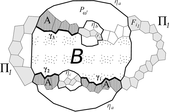
Figure 32: The belt $\mathcal{B}_{l}$ intersecting $P_{\omega^{r}}$

Then $A\cdot B=[\gamma_{1}]+\dots+[\gamma_{q}]$, where $\gamma_{i}$ is an edge path in $P_{\omega^{r}}$ that starts at $\eta_{\alpha_{i-1}}$ and ends at $\eta_{\alpha_{i}}$, $\alpha_{j}\in[s]$, $j=0,\dots,q$, $i=1,\dots,q$, and $\{\alpha_{0},\alpha_{q}\}=\{a,b\}$. This element corresponds to a path connecting $\eta_{a}$ and $\eta_{b}$ in $P_{\omega^{r}}$. Thus we can realize any element from the basis given by Proposition 6.7.

The following simple result is well-known.

Lemma 7.13.

Simplex $\Delta^{3}$ is rigid in the class of all simple $3$-polytopes.

Proof 7.14.

This is equivalent to the fact that any two facets intersect, that is $H^{3}(\mathcal{Z}_{P})=0$.

The following result follows from Theorem 5.7 in [24]. We will give another proof here.

Theorem 7.15.

The polytope $P\neq\Delta^{3}$ is flag if and only if

$$H^{m-2}(\mathcal{Z}_{P})\subset(\widetilde{H}^{*}(\mathcal{Z}_{P}))^{2}.$$

Proof 7.16.

The polytope $P\neq\Delta^{3}$ is not flag if and only if it has a $3$-belt. This corresponds to an element of a basis in $H^{-1,2\omega}(\mathcal{Z}_{P})\simeq H_{1}(P_{\omega},\partial P_{\omega})$, $|\omega|=3$. By the Poincare duality this element corresponds to an element of a basis in $H^{-(m-4),2([m]\setminus\omega)}(\mathcal{Z}_{P})\simeq\widehat{H}_{2}(P_{\omega},\partial P_{\omega})$. The latter element belongs to $H^{m-2}(\mathcal{Z}_{P})$ but does not belong to $(\widetilde{H}^{*}(\mathcal{Z}_{P}))^{2}$.

If the polytope is flag, then it has no $3$-belts, and by Proposition 6.14

$$H^{5}(\mathcal{Z}_{P})=\bigoplus\limits_{|\omega|=4}H^{-3,2\omega}(\mathcal{Z}_{P})=\bigoplus\limits_{|\omega|=4}\widehat{H}_{2}(P_{\omega},\partial P_{\omega}).$$

Hence by the Poincare duality

$$H^{m-2}(\mathcal{Z}_{P})=\bigoplus\limits_{|\omega|=m-4}H_{1}(P_{\omega},\partial P_{\omega}).$$

By Corollary 7.11 we have $H^{m-2}(\mathcal{Z}_{P})\subset(\widetilde{H}^{*}(\mathcal{Z}_{P}))^{2}$.

By Lemma 7.13 the simplex is a rigid polytope. This finishes the proof.

Corollary 7.17.

The property to be a flag polytope is rigid in the class of simple $3$-polytopes.

4 Rigidity of the property to have a $4$-belt

Remind that for any set $\omega=\{i,j\}\subset[m]$ we have

$$H^{-1,2\omega}(\mathcal{Z}_{P})=\widehat{H}_{2}(P_{\omega},\partial P_{\omega})=\begin{cases}\mathbb{Z}\text{ with generator }[F_{i}]=-[F_{j}],&F_{i}\cap F_{j}=\varnothing,\\ 0,&F_{i}\cap F_{j}\neq\varnothing,\end{cases}$$

and

$$H^{3}(\mathcal{Z}_{P})=\bigoplus\limits_{\{i,j\}\colon F_{i}\cap F_{j}=\varnothing}\mathbb{Z}$$

Definition 7.18.

The set $\{F_{i_{1}},\dots,F_{i_{k}}\}$ with $F_{i_{1}}\cap\dots\cap F_{i_{k}}=\varnothing$ is called a nonface of $P$, and the corresponding set $\{i_{1},\dots,i_{k}\}$ – a nonface of $K_{P}$. A nonface minimal by inclusion is called a minimal nonface. Define $N(K)$ to be the set of all minimal nonfaces of the simplicial complex $K$.

For any nonface $\omega=\{i,j\}$ choose a generator $\widetilde{\omega}\in H^{-1,2\omega}(\mathcal{Z}_{P})$.

Proposition 7.19.

The multiplication $H^{3}(\mathcal{Z}_{P})\otimes H^{3}(\mathcal{Z}_{P})\to H^{6}(\mathcal{Z}_{P})$ is trivial if and only if $P$ has no $4$-belts.

Proof 7.20.

For $\omega_{1}=\{i,j\},\omega_{2}=\{p,q\}\in N(K_{P})$, $\omega_{1}\cap\omega_{2}=\varnothing$, the simplicial complex $K_{\omega_{1}\sqcup\omega_{2}}$ has no $2$-simplices; hence it is at most $1$-dimensional and can be considered as a graph. Moreover, this graph has no $3$-cycles. If it has a $4$-cycle, then $K_{\omega_{1}\sqcup\omega_{2}}$ is a boundary of a $4$-gon, $(F_{i},F_{p},F_{j},F_{q})$ is a $4$-belt, and $\widetilde{\omega_{1}}\cdot\widetilde{\omega_{2}}$ is a generator of $H_{1}(P_{\omega_{1}\sqcup\omega_{2}},\partial P_{\omega_{1}\sqcup\omega_{2}})$. If $K_{\omega_{1}\sqcup\omega_{2}}$ has no $4$-cycles, then it has no cycles at all, $H_{1}(P_{\omega_{1}\sqcup\omega_{2}},\partial P_{\omega_{1}\sqcup\omega_{2}})\simeq\widetilde{H}^{1}(K_{\omega_{1}\sqcup\omega_{2}})=0$, and $\widetilde{\omega_{1}}\cdot\widetilde{\omega_{2}}=0$. This proves the statement.

Corollary 7.21.

The property to have a $4$-belt is rigid in the class of all simple $3$-polytopes.

5 Rigidity of flag $3$-polytopes without $4$-belts

First we prove the following technical result, which we will need below.

Proposition 7.22.

(Lemma 3.2, [23]) Let $P$ be a flag $3$-polytope without $4$-belts. Then for any three different facets $\{F_{i},F_{j},F_{k}\}$ with $F_{i}\cap F_{j}=\varnothing$ there exist $l\geqslant 5$ and an $l$-belt $\mathcal{B}_{l}$ such that $F_{i},F_{j}\in\mathcal{B}_{l}$, $F_{k}\notin\mathcal{B}_{l}$, and $F_{k}$ does not intersect at least one of the two connected components of $\mathcal{B}_{l}\setminus\{F_{i},F_{j}\}$.

Remark 7.23.

In [23] only the sketch of the proof is given. It contains several additional assumptions. We give the full prove following the same idea.

Proof 7.24.

From Proposition 7.9 there is an $s$-belt $\mathcal{B}_{1}$, with $F_{i},F_{j}\in\mathcal{B}_{1}\not\ni F_{k}$. We have $\mathcal{B}_{1}=(F_{i},F_{i_{1}},\dots,F_{i_{p}},F_{j},F_{j_{1}},\dots,F_{j_{q}})$, $s=p+q+2$, $p,q\geqslant 1$. According to Lemma 3.9 the belt $\mathcal{B}_{1}$ divides the surface $\partial P\setminus\mathcal{B}_{1}$ into two connected components $\mathcal{P}_{1}$ and $\mathcal{P}_{2}$, both homeomorphic to disks. Consider the component $\mathcal{P}_{\alpha}$ containing ${\rm int}\,F_{k}$. Set $\beta=3-\alpha$. Then either $\partial\mathcal{P}_{\alpha}=\partial F_{k}$, or $\partial\mathcal{P}_{\alpha}\cap\partial F_{k}$ consists of finite set of disjoint edge-segments $\gamma_{1}$, $\dots$, $\gamma_{d}$.

Figure 33: Case 1

Consider the first case. Then $\mathcal{B}_{1}$ surrounds $F_{k}$, and $F_{i}$ and $F_{j}$ are adjacent to $F_{k}$. Consider all facets $\{F_{w_{1}},\dots,F_{w_{r}}\}$ in $\mathcal{W}_{\beta}$ (in the notations of Lemma 3.9), adjacent to facets in $\{F_{i_{1}},\dots,F_{i_{p}}\}$ (see Fig. 33), in the order we meet them while walking round $\partial\mathcal{B}_{1}$ from $F_{i}$ to $F_{j}$. Then $F_{w_{a}}\cap F_{j_{b}}=\varnothing$ for any $a,b$, else $(F_{k},F_{j_{b}},F_{w_{a}},F_{i_{c}})$ is a $4$-belt for any $i_{c}$ with $F_{i_{c}}\cap F_{w_{a}}\neq\varnothing$, since $F_{k}\cap F_{w_{a}}=\varnothing$ (because ${\rm int}\,F_{w_{a}}\subset\mathcal{P}_{\beta}$) and $F_{j_{b}}\cap F_{i_{c}}=\varnothing$. We have a thick path $(F_{i},F_{w_{1}},\dots,F_{w_{r}},F_{j})$. Consider the shortest thick path of the form $(F_{i},F_{w_{s_{1}}},\dots,F_{w_{s_{t}}},F_{j})$. If two facets of this path intersect, then they are successive, else there is a shorter thick path. Thus we have a belt $(F_{i},F_{w_{s_{1}}},\dots,F_{w_{s_{t}}},F_{j},F_{j_{1}},\dots,F_{j_{q}})$ containing $F_{i}$, $F_{j}$, not containing $F_{k}$, and the segment $(F_{w_{s_{1}}},\dots,F_{w_{s_{t}}})$ does not intersect $F_{k}$.

Now consider the second case. We can assume that $F_{i}\cap F_{k}=\varnothing$ or $F_{j}\cap F_{k}=\varnothing$, say $F_{i}\cap F_{k}\neq\varnothing$, else consider the belt $\mathcal{B}_{1}$ surrounding $F_{k}$ and apply the arguments of the first case. Let $\gamma_{a}=(F_{k}\cap F_{u_{a,1}},\dots,F_{k}\cap F_{u_{a,l_{a}}})$. Set $\mathcal{U}_{a}=(F_{u_{a,1}},\dots,F_{u_{a,l_{a}}})$. The segment $(F_{s_{a,1}},\dots,F_{s_{a,t_{a}}})$ of $\mathcal{B}_{1}$ between $\mathcal{U}_{a}$ and $\mathcal{U}_{a+1}$ denote $\mathcal{S}_{a}$. Then $\mathcal{B}_{1}=(\mathcal{U}_{1},\mathcal{S}_{1},\mathcal{U}_{2},\dots,\mathcal{U}_{d},\mathcal{S}_{d})$ for some $d$.

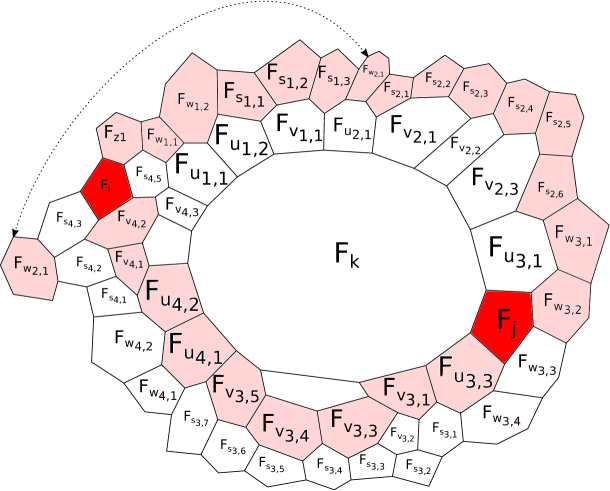
Figure 35: Modified belt

Consider the thick path $W_{a}=(F_{w_{a,1}},\dots,F_{w_{a,r_{a}}})\subset\mathcal{W}_{\beta}$ (see notation in Lemma 3.9) arising while walking round the facets in $\mathcal{W}_{\beta}$ intersecting facets in $\mathcal{U}_{a}$ (see Fig. 35). Then $W_{a}\cap W_{b}=\varnothing$ for $a\neq b$, else $(F_{w},F_{u_{a,j_{1}}},F_{k},F_{u_{b,j_{2}}})$ is a $4$-belt for any $F_{w}\in W_{a}\cap W_{b}$ such that $F_{w}\cap F_{u_{a,j_{1}}}\neq\varnothing$, $F_{w}\cap F_{u_{b,j_{2}}}\neq\varnothing$. Also $F_{w_{a,j_{1}}}\neq F_{w_{a,j_{2}}}$ for $j_{1}\neq j_{2}$. This is true for facets adjacent to the same facet $F_{u_{a,i}}$. Let $F_{w_{a,j_{1}}}=F_{w_{a,j_{2}}}$. If the facets are adjacent to the successive facets $F_{u_{a,i}}$ and $F_{u_{a,i+1}}$, then the flagness condition implies that $j_{1}=j_{2}$ and $F_{w_{a,j_{1}}}$ is the facet in $\mathcal{W}_{\beta}$ intersecting $F_{u_{a,i}}\cap F_{u_{a,i+1}}$. If the facets are adjacent to non-successive facets $F_{u_{a,i}}$ and $F_{u_{a,j}}$, then $(F_{w_{a,j_{1}}},F_{u_{a,i}},F_{k},F_{u_{a,j}})$ is a $4$-belt, which is a contradiction.

Now consider the thick path $\mathcal{V}_{b}=(F_{v_{b,1}},\dots,F_{v_{b,c_{b}}})$ arising while walking round the facets in $\mathcal{W}_{\alpha}$ intersecting facets in $\mathcal{S}_{b}$ (see Fig. 35). Then $\mathcal{V}_{a}\cap\mathcal{V}_{b}=\varnothing$ for $a\neq b$, and $W_{a}\cap\mathcal{V}_{b}=\varnothing$ for any $a,b$, since interiors of the corresponding facets lie in different connected components of $\partial P\setminus(\mathcal{B}_{1}\cup F_{k})$, moreover by the same reason we have $F_{v_{a,j}}\cap F_{v_{b,j}}=\varnothing$ for any $i,j$, and $a\neq b$.

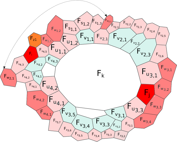
Figure 34: Case 2

Now we will deform the segments $\mathcal{I}=(F_{i_{1}},\dots,F_{i_{p}})$ and $\mathcal{J}=(F_{j_{1}},\dots,F_{j_{q}})$ of the belt $\mathcal{B}_{1}$ to obtain a new belt $(F_{i},\mathcal{I}^{\prime},F_{j},\mathcal{J}^{\prime})$ with $\mathcal{I}^{\prime}$ not intersecting $F_{k}$. First substitute the thick path $W_{a}$ for each segment $\mathcal{U}_{a}\subset\mathcal{I}$ and the thick path $\mathcal{V}_{b}$ for each segment $\mathcal{S}_{b}\subset\mathcal{J}$. Since $F_{s_{a,t_{a}}}\cap F_{w_{a+1,1}}\neq\varnothing$, $F_{w_{a,r_{a}}}\cap F_{s_{a,1}}\neq\varnothing$, $F_{v_{a,c_{a}}}\cap F_{u_{a+1,1}}\neq\varnothing$, and $F_{u_{a,l_{a}}}\cap F_{s_{a,1}}\neq\varnothing$ for any $a$ and $a+1$ considered $\mod d$, we obtain a loop $\mathcal{L}_{1}=(F_{i},\mathcal{I}_{1},F_{j},\mathcal{J}_{1})$ instead of $\mathcal{B}_{1}$.

Since $F_{i}\cap F_{k}=\varnothing$, we have $F_{i}=F_{s_{a_{i},f_{i}}}$ for some $a_{i},f_{i}$. If $F_{j}=F_{s_{a_{j},f_{j}}}$ for some $a_{j},f_{j}$, then we can assume that $a_{i}\neq a_{j}$, else the facets in $\mathcal{I}$ or $\mathcal{J}$ already do not intersect $F_{k}$, and $\mathcal{B}_{1}$ is the belt we need. If $F_{j}=F_{u_{a_{j},f_{j}}}$ for some $a_{j}$ and some $f_{j}>1$, then substitute the thick path $(F_{w_{a_{j},1}},\dots,F_{w_{a_{j},g_{j}}})$, where $g_{j}$ – the first integer with $F_{w_{a_{j},g_{j}}}\cap F_{j}\neq\varnothing$ (then $F_{j}\cap F_{u_{a_{j},f_{j}-1}}\cap F_{w_{a_{j},g_{j}}}$ is a vertex), for the segment $(F_{u_{a_{j},1}},\dots,F_{u_{a_{j},f_{j}-1}})$ to obtain a loop $\mathcal{L}_{2}=(F_{i},\mathcal{I}_{2},F_{j},\mathcal{J}_{1})$ (else set $\mathcal{L}_{2}=\mathcal{L}_{1}$) with facets in $\mathcal{I}_{2}$ not intersecting $F_{k}$. If $f_{j}<l_{a_{j}}$, then $F_{w_{a_{j},g_{j}}}\cap F_{u_{a_{j},f_{j}+1}}=\varnothing$, else $(F_{k},F_{u_{a_{j},f_{j}-1}},F_{w_{a_{j},g_{j}}},F_{u_{a_{j},f_{j}+1}})$ is a $4$-belt. Then $F_{w_{a,l}}\cap F_{u_{a_{j},r}}=\varnothing$ for any $r\in\{f_{j}+1,\dots,l_{a_{j}}\}$ and $a,l$, such that either $a\neq a_{j}$, or $a=a_{j}$, and $l\in\{1,\dots,g_{j}\}$. Hence facets of the segment $(F_{u_{a_{j},f_{j}+1}},\dots,F_{u_{a_{j},l_{a_{j}}}})$ do not intersect facets in $\mathcal{I}_{2}$.

Now a facet $F_{i_{a}^{\prime}}$ of $\mathcal{I}_{2}$ can intersect a facet $F_{j_{b}^{\prime}}$ of $\mathcal{J}_{1}$ only if $F_{i_{a}^{\prime}}=F_{w_{c,h}}$ for some $c,h$, and $F_{j_{b}^{\prime}}=F_{s_{a_{i},l}}$ for $l<f_{i}$, or $F_{j_{b}^{\prime}}=F_{s_{a_{j},l}}$ for $F_{j}=F_{s_{a_{j},f_{j}}}$ and $l>f_{j}$. In the first case take the smallest $l$ for all $c,h$, and the correspondent facet $F_{w_{c,h}}$. Consider the facet $F_{u_{b,g}}=F_{i_{e}}\in\mathcal{I}$ with $F_{u_{b,g}}\cap F_{w_{c,h}}\neq\varnothing$. Then $\mathcal{L}^{\prime}=(F_{s_{a_{i},l}},F_{s_{a_{i},l+1}},\dots,F_{i},F_{i_{1}},\dots,F_{i_{e}},F_{w_{c,h}})$ is a simple loop. If $f_{i}<t_{a_{i}}$, then consider the thick path $\mathcal{Z}_{1}=(F_{z_{1,1}},\dots,F_{z_{1,y_{1}}})$ arising while walking along the boundary of $\mathcal{B}_{1}$ in $\mathcal{W}_{\beta}$ from the facet $F_{z_{1,1}}$ intersecting $F_{i}\cap F_{i_{1}}$ by the vertex, to the facet $F_{z_{1,y_{1}}}$ preceding $F_{w_{a_{i}+1,1}}$. Consider the thick path $\mathcal{X}_{1}=(F_{v_{a_{i},1}},\dots,F_{v_{a_{i},x_{1}}})$ with $x_{1}$ being the first integer with $F_{v_{a_{i},x_{1}}}\cap F_{i}\neq\varnothing$. Consider the simple curve $\eta\subset\partial P$ consisting of segments connecting the midpoints of the successive edges of intersection of the successive facets of $\mathcal{L}^{\prime}$. It divides $\partial P$ into two connected components $\mathcal{E}_{1}$ and $\mathcal{E}_{2}$ with $\mathcal{J}_{1}\setminus(F_{s_{a_{i},l}},\dots,F_{s_{a_{i},f_{i}-1}})$ lying in one connected component $\mathcal{E}_{\alpha}$, and $\mathcal{Z}_{1}$ – in $\mathcal{E}_{\beta}\cup F_{w_{c,h}}$, $\beta=3-\alpha$. Now substitute $\mathcal{X}_{1}$ for the segment $(F_{s_{a_{i},1}},\dots,F_{s_{a_{i},f_{i}-1}})$ of $\mathcal{J}_{1}$. If $f_{i}<t_{a_{i}}$ substitute $\mathcal{Z}_{1}$ for the segment $(F_{s_{a_{i},f_{i}+1}},\dots,F_{s_{a_{i},t_{a_{i}}}})$ of $\mathcal{I}_{2}$ to obtain a new loop $(F_{i},\mathcal{I}_{3},F_{j},\mathcal{J}_{2})$ with facets in $\mathcal{I}_{3}$ not intersecting $F_{k}$. A facet $F_{i_{a}}^{\prime\prime}$ in $\mathcal{I}_{3}$ can intersect a facet $F_{j_{b}}^{\prime\prime}$ in $\mathcal{J}_{2}$ only if $F_{i_{a}^{\prime\prime}}=F_{w_{c^{\prime},h^{\prime}}}$ for some $c^{\prime},h^{\prime}$, $F_{j}=F_{s_{a_{j},f_{j}}}$, and $F_{j_{b}^{\prime\prime}}=F_{s_{a_{j},l}}$ for $l>f_{j}$. The thick path $\mathcal{Z}_{1}$ lies in $\mathcal{E}_{\beta}\cup F_{w_{c,h}}$ and the segment $(F_{j}=F_{s_{a_{j},f_{j}}},\dots,F_{s_{a_{j},t_{a_{j}}}})$ lies in $\mathcal{E}_{\alpha}$; hence intersections of facets in $\mathcal{I}_{3}$ with facets in $\mathcal{J}_{2}$ are also intersections of the same facets in $\mathcal{I}_{2}$ and $\mathcal{J}_{1}$, and $F_{w_{c^{\prime},h^{\prime}}}$ is either $F_{w_{c,h}}$, or lies in $\mathcal{E}_{\alpha}$. We can apply the same argument for $\mathcal{S}_{a_{j}}$ as for $\mathcal{S}_{a_{i}}$ to obtain a new loop $\mathcal{L}_{4}=(F_{i},\mathcal{I}_{4},F_{j},\mathcal{J}_{3})$ with facets in $\mathcal{I}_{4}$ not intersecting $F_{k}$ and facets in $\mathcal{J}_{3}$. Then take the shortest thick path from $F_{i}$ to $F_{j}$ in $F_{i}\cup\mathcal{I}_{4}\cup F_{j}$ and the shortest thick path from $F_{j}$ to $F_{i}$ in $F_{j}\cup\mathcal{J}_{3}\cup F_{i}$ to obtain the belt we need.

Definition 7.25.

An annihilator of an element $r$ in a ring $R$ is defined as

$${\rm Ann}_{R}(r)=\{s\in R\colon rs=0\}$$

Proposition 7.26.

The set of elements in $H^{3}(\mathcal{Z}_{P})$ corresponding to

$$\bigcup\limits_{\{i,j\}\colon F_{i}\cap F_{j}=\varnothing}\{[F_{i}],[F_{j}]\in\widehat{H}_{2}(P_{\{i,j\}},\partial P_{\{i,j\}})\}$$

is rigid in the class of all simple flag $3$-polytopes without $4$-belts.

Proof 7.27.

Since the group $H^{*}(\mathcal{Z}_{P})$ has no torsion, we have the isomorphism $H^{*}(\mathcal{Z}_{P},\mathbb{Q})\simeq H^{*}(\mathcal{Z}_{P})\otimes\mathbb{Q}$ and the embedding $H^{*}(\mathcal{Z}_{P})\subset H^{*}(\mathcal{Z}_{P})\otimes\mathbb{Q}$. For polytopes $P$ and $Q$ the isomorphism $H^{*}(\mathcal{Z}_{P})\simeq H^{*}(\mathcal{Z}_{Q})$ implies the isomorphism over $\mathbb{Q}$. For the cohomology over $\mathbb{Q}$ all theorems about structure of $H^{*}(\mathcal{Z}_{P},\mathbb{Q})$ are still valid. In what follows we consider cohomology over $\mathbb{Q}$. Set $H=H^{*}(\mathcal{Z}_{P},\mathbb{Q})$. We will need the following result.

Lemma 7.28.

For an element

$$\alpha=\sum\limits_{\omega\in N(K_{P}),|\omega|=2}r_{\omega}\widetilde{\omega}\quad\text{with }|\{\omega\colon r_{\omega}\neq 0\}|\geqslant 2$$

we have

$$\dim{\rm Ann}_{H}(\alpha)<\dim{\rm Ann}_{H}(\widetilde{\omega}),\text{ if }r_{\omega}\neq 0.$$

Proof 7.29.

Choose a complementary subspace $C_{\omega}$ to ${\rm Ann}_{H}(\widetilde{\omega})$ in $H$ as a direct sum of complements $C_{\omega,\tau}$ to ${\rm Ann}_{H}(\widetilde{\omega})\cap\widehat{H}_{*}(P_{\tau},\partial P_{\tau})$ in $\widehat{H}_{*}(P_{\tau},\partial P_{\tau})$ for all $\tau\subset[m]\setminus\omega$. Then for any $\beta\in C_{\omega}\setminus\{0\}$ we have $\beta\widetilde{\omega}\neq 0$, which is equivalent to the fact that $\beta=\sum\limits\beta_{\tau}$, $\beta_{\tau}\in C_{\omega,\tau}$, $\tau\subset[m]\setminus\omega$, with $\beta_{\tau_{\beta}}\widetilde{\omega}\neq 0$ for some $\tau_{\beta}\subset[m]\setminus\omega$. Moreover for any $\omega^{\prime}\neq\omega$ with $r_{\omega^{\prime}}\neq 0$ and $\tau\subset[m]\setminus\omega$, $\tau\neq\tau_{\beta}$, we have $\tau_{\beta}\sqcup\omega\notin\{\tau\cup\omega^{\prime},\tau_{\beta}\cup\omega^{\prime},\tau\sqcup\omega\}$; hence $(\beta\cdot\alpha)_{\tau_{\beta}\sqcup\omega}=r_{\omega}\beta_{\tau_{\beta}}\cdot\widetilde{\omega}\neq 0$, and $\beta\alpha\neq 0$. Then $C_{\omega}$ forms a direct sum with ${\rm Ann}(\alpha)$. Now consider some $\omega^{\prime}\neq\omega$, $|\omega^{\prime}|=2$, $r_{\omega^{\prime}}\neq 0$. Let $\omega=\{p,q\}$, $\omega^{\prime}=\{s,t\}$, $q\notin\omega^{\prime}$. By Proposition 7.22 there is an $l$-belt $\mathcal{B}_{l}$ such that $F_{s},F_{t}\in\mathcal{B}_{l}$, $F_{q}\notin\mathcal{B}_{l}$, and $F_{q}$ does not intersect one of the two connected components $B_{1}$ and $B_{2}$ of $\mathcal{B}_{l}\setminus\{F_{s},F_{t}\}$, say $B_{1}$. Take $\xi=[\sum\limits_{i\colon F_{i}\subset B_{1}}F_{i}]\in\widehat{H}_{2}(P_{\tau},\partial P_{\tau}),\,\tau=\{i\colon F_{i}\in\mathcal{B}_{l}\setminus\{F_{s},F_{t}\}\}$,and $[F_{s}]\in\widehat{H}_{2}(P_{\omega^{\prime}},\partial P_{\omega^{\prime}})$. Then $\xi\cdot[F_{s}]$ is a generator in $H_{1}(\mathcal{B}_{l},\partial\mathcal{B}_{l})\simeq\mathbb{Z}$. On the other hand, take $[F_{q}]\in\widehat{H}_{2}(P_{\omega},\partial P_{\omega})$. Then either $F_{p}\in\mathcal{B}_{l}\setminus\{F_{s},F_{t}\}$, and $\xi\cdot\widetilde{\omega}=0$, since $\tau\cap\omega\neq\varnothing$, or $F_{p}\notin\mathcal{B}_{l}\setminus\{F_{s},F_{t}\}$, and $\pm\xi\cdot\widetilde{\omega}=\xi\cdot[F_{q}]=0$, since $F_{q}$ does not intersect $B_{1}$. In both cases $\xi\in{\rm Ann}(\widetilde{\omega})$ and $\xi\cdot\widetilde{\omega^{\prime}}\neq 0$. Then $\xi\cdot\alpha\neq 0$, since $\tau\sqcup\omega^{\prime}\neq\tau\sqcup\omega_{1}$ for $\omega_{1}\neq\omega^{\prime}$. Consider any $\beta=\sum\limits_{\tau\subset[m]\setminus\omega}\beta_{\tau}\in C_{\omega}\setminus\{0\}$. We have $(\beta\cdot\alpha)_{\tau_{\beta}\sqcup\omega}\neq 0$. If $(\xi\cdot\alpha)_{\tau_{\beta}\sqcup\omega}\neq 0$, then since $\xi$ is a homogeneous element, $(\xi\cdot\alpha)_{\tau_{\beta}\sqcup\omega}=r_{\omega_{1}}\xi\cdot\widetilde{\omega_{1}}$ for $\omega_{1}=(\tau_{\beta}\sqcup\omega)\setminus\tau=\{q,r\}$, $r\in[m]$. We have $\xi\cdot\widetilde{\omega_{1}}=\pm\xi\cdot[F_{q}]=0$, since $F_{q}$ does not intersect $B_{1}$. A contradiction. Thus, $((\xi+\beta)\cdot\alpha)_{\tau_{\beta}\sqcup\omega}=(\beta\cdot\alpha)_{\tau_{\beta}\sqcup\omega}\neq 0$; hence $(\xi+\beta)\cdot\alpha\neq 0$, and the space $\langle\xi\rangle\oplus C_{\omega}$ forms a direct sum with ${\rm Ann}_{H}(\alpha)$. This finishes the proof.

Now let us prove Proposition 7.26. Let $\varphi\colon H^{*}(\mathcal{Z}_{P},\mathbb{Z})\to H^{*}(\mathcal{Z}_{Q},\mathbb{Z})$ be an isomorphism of graded rings for flag simple $3$-polytopes $P$ and $Q$ without $4$-belts. Let $\omega\in N(K_{P})$, $|\omega|=2$, and

$$\varphi(\widetilde{\omega})=\alpha=\sum\limits_{\omega^{\prime}\in N(K_{Q}),|\omega^{\prime}|=2}r_{\omega^{\prime}}\widetilde{\omega^{\prime}}\text{ with }|\{\omega^{\prime}\colon r_{\omega^{\prime}}\neq 0\}|\geqslant 2.$$

Then there is some $\omega^{\prime}$ such that $r_{\omega^{\prime}}\neq 0$ and $\varphi^{-1}(\widetilde{\omega^{\prime}})=\alpha^{\prime}=\sum\limits_{\omega^{\prime\prime}\in N(K_{P}),|\omega^{\prime\prime}|=2}r^{\prime}_{\omega^{\prime\prime}}\widetilde{\omega^{\prime\prime}}$ with $r^{\prime}_{\omega}\neq 0$. Now consider all the mappings in cohomology over $\mathbb{Q}$. Since dimension of annihilator of an element is invariant under isomorphisms,Lemma 7.28 gives a contradiction:

$$\dim{\rm Ann}(\widetilde{\omega})=\dim{\rm Ann}(\alpha)<\dim{\rm Ann}(\widetilde{\omega^{\prime}})=\dim{\rm Ann}(\alpha^{\prime})<\dim{\rm Ann}(\widetilde{\omega}).$$

Thus $\varphi(\widetilde{\omega})=r_{\omega^{\prime}}\widetilde{\omega^{\prime}}$ for some $\omega^{\prime}$. Since the isomorphism is over $\mathbb{Z}$, we have $r_{\omega^{\prime}}=\pm 1$. This finishes the proof.

Definition 7.30.

Following [24] and [23] for a graded algebra $A=\bigoplus\limits_{i\geqslant 0}A^{i}$ over the field $k$, and a nonzero element $\alpha\in A$ define a $p$-factorspace $V$ to be a vector subspace in $A^{p}$ such that for any $v\in V\setminus\{0\}$ there exists $u_{v}\in A$ with $vu_{v}=\alpha$. A $p$-factorindex ${\rm ind}_{p}(\alpha)$ is defined to be the maximal dimension of $p$-factorspaces of $\alpha$.

Definition 7.31.

Define $\mathbf{B}_{k}=\bigoplus\limits_{\mathcal{B}_{k}-\text{$k$-belt}}H_{1}(\mathcal{B}_{k},\partial\mathcal{B}_{k})$ to be the subgroup in $H^{k+2}(\mathcal{Z}_{P})$ generated by all elements $\widetilde{\mathcal{B}_{k}}$ corresponding to $k$-belts.

Definition 7.32.

For the rest of the Section let $\{\omega_{i}\}_{i=1}^{N(P)}$ be the set of all missing edges of the complex $K_{P}$ of the polytope $P$.

Proposition 7.33.

Let $P$ be a simple $3$-polytope. Then

1. for any element $\alpha\in H^{k+2}(\mathcal{Z}_{P},\mathbb{Q})$, $4\leqslant k\leqslant m-2$, we have ${\rm ind}_{3}(\alpha)\leqslant\frac{k(k-3)}{2}$, and the equality ${\rm ind}_{3}(\alpha)=\frac{k(k-3)}{2}$ implies $\alpha\in(\mathbf{B}_{k}\otimes\mathbb{Q})\setminus\{0\}$.

2. for any $k$-belt $\mathcal{B}_{k}$, $4\leqslant k\leqslant m-2$, we have ${\rm ind}_{3}(\widetilde{\mathcal{B}_{k}})=\frac{k(k-3)}{2}$;

In particular, the group $\mathbf{B}_{k}\subset H^{k+2}(\mathcal{Z}_{P},\mathbb{Z})$, $4\leqslant k\leqslant m-2$, is $B$-rigid in the class of all simple $3$-polytopes.

Proof 7.34.

(1) We have

$$\alpha=\sum\limits_{\omega}\alpha_{\omega}\in\bigoplus\limits_{|\omega|=k}H_{1}(P_{\omega},\partial P_{\omega},\mathbb{Q})\oplus\bigoplus\limits_{|\omega|=k+1}\widehat{H}_{2}(P_{\omega},\partial P_{\omega},\mathbb{Q}),$$

Let $0\neq\beta=\sum\limits_{i=1}^{N(P)}\lambda_{i}\widetilde{\omega}_{i}$ be the divisor of $\alpha$. Then there exists

$$\gamma=\sum\limits_{\eta}\gamma_{\eta}\in\bigoplus\limits_{|\eta|=k-3}H_{1}(P_{\eta},\partial P_{\eta},\mathbb{Q})\oplus\bigoplus\limits_{|\eta|=k-2}\widehat{H}_{2}(P_{\eta},\partial P_{\eta},\mathbb{Q}),$$

with $\beta\cdot\gamma=\alpha$. Then $\alpha_{\omega}=0$, for all $\omega$ with $|\omega|=k+1$, $\gamma_{\eta}=0$ for all $\eta$ with $|\eta|=k-3$, and $\alpha_{\omega}=\sum\limits_{\omega_{i}\subset\omega}\lambda_{i}\widetilde{\omega_{i}}\cdot\gamma_{\omega\setminus\omega_{i}}=\left(\sum\limits_{\omega_{i}\subset\omega}\lambda_{i}\widetilde{\omega_{i}}\right)\cdot\left(\sum\limits_{\eta\subset\omega,|\eta|=k-2}\gamma_{\eta}\right)$. Thus for any $3$-factorspace $V$ of $\alpha$ and any $\omega$ with $\alpha_{\omega}\neq 0$ the linear mapping

$$\varphi_{\omega}\colon V\to H^{3}(\mathcal{Z}_{P},\mathbb{Q})\colon\beta\to\beta_{\omega}=\sum\limits_{\omega_{i}\subset\omega}\lambda_{i}\widetilde{\omega_{i}}$$

is a monomorphism; hence it is a linear isomorphism of $V$ to the factorspace $\varphi_{\omega}(V)$ of $\alpha_{\omega}$. Let $P_{\omega}=P_{\omega^{1}}\sqcup\dots\sqcup P_{\omega^{s}}$ be the decomposition into the connected components. Then $H_{1}(P_{\omega},\partial P_{\omega})=\bigoplus\limits_{l=1}^{s}H_{1}(P_{\omega^{l}},\partial P_{\omega^{l}})$, and $\alpha_{\omega}=\sum\limits_{l=1}^{s}\alpha_{\omega^{l}}$. Let $\omega_{i}=\{p,q\}$, with $p\in\omega^{a}$, $q\in\omega^{b}$. If $a\neq b$, then $\widetilde{\omega_{i}}\cdot\gamma_{\omega\setminus\omega_{i}}=0$, since $\widetilde{\omega_{i}}=\pm[F_{p}]=\mp[F_{q}]$, and the cohomology class $\widetilde{\omega_{i}}\cdot\gamma_{\omega\setminus\omega_{i}}$ should lie in $H_{1}(P_{\omega^{a}},\partial P_{\omega^{a}})\cap H_{1}(P_{\omega^{b}},\partial P_{\omega^{b}})=0$. Consider $\omega_{i}=\{p,q\}\subset\omega^{a}$. Each connected component of $P_{\omega\setminus\omega_{i}}$ lies in some $P_{\omega^{l}}$. We have $\gamma_{\omega\setminus\omega_{i}}=\sum\limits_{l=1}^{s}\gamma_{\omega^{l}\setminus\omega_{i}}$, where each summand corresponds to the connected components lying in $\omega^{l}\setminus\omega_{i}$. Since $\widetilde{\omega_{i}}\cdot\gamma_{\omega^{l}\setminus\omega_{i}}=0$ for $l\neq a$, we have

$$\sum\limits_{l=1}^{s}\alpha_{\omega^{l}}=\alpha_{\omega}=\left(\sum\limits_{l=1}^{s}\sum\limits_{\omega_{i}\subset\omega^{l}}\lambda_{i}\widetilde{\omega_{i}}+\sum\limits_{\omega_{i}\not\subset\omega^{l}\forall l}\lambda_{i}\widetilde{\omega_{i}}\right)\cdot\left(\sum\limits_{\omega_{i}\subset\omega}\gamma_{\omega\setminus\omega_{i}}\right)=\\ \left(\sum\limits_{l=1}^{s}\sum\limits_{\omega_{i}\subset\omega^{l}}\lambda_{i}\widetilde{\omega_{i}}\right)\cdot\left(\sum\limits_{l=1}^{s}\sum\limits_{\omega_{j}\subset\omega^{l}}\gamma_{\omega^{l}\setminus\omega_{j}}\right)=\sum\limits_{l=1}^{s}\left(\sum\limits_{\omega_{i}\subset\omega^{l}}\lambda_{i}\widetilde{\omega_{i}}\right)\cdot\left(\sum\limits_{\omega_{j}\subset\omega^{l}}\gamma_{\omega^{l}\setminus\omega_{j}}\right);$$

hence for any $\alpha_{\omega^{l}}\neq 0$ the projection $\psi_{l}\colon\sum\limits_{\omega_{i}\subset\omega}\lambda_{i}\widetilde{\omega_{i}}\to\sum\limits_{\omega_{i}\subset\omega^{l}}\lambda_{i}\widetilde{\omega_{i}}$ sends the space $\varphi_{\omega}(V)$ isomorphically to the $3$-factorspace $\psi_{l}\varphi_{\omega}(V)$ of $\alpha_{\omega^{l}}$. Now consider the connected space $P_{\omega^{l}}$.

Let the graph $K^{1}_{\omega^{l}}$ have a hanging vertex $a$. Then the facet $F_{a}$ intersects only one facet among $\{F_{t}\}_{t\in\omega^{l}\setminus\{a\}}$, say $F_{b}$. Then for any $\omega_{i}=\{a,r\}\subset\omega^{l}$ we have $\widetilde{\omega_{i}}\cdot\gamma_{\omega^{l}\setminus\omega_{i}}=\pm[F_{a}]\cdot\gamma_{\omega^{l}\setminus\omega_{i}}$ is equal up to a scalar to the class in $H_{1}(P_{\omega^{l}},\partial P_{\omega^{l}},\mathbb{Q})$ of the single edge $F_{a}\cap F_{b}$ connecting two points on the same boundary cycle of $P_{\omega^{l}}$. Hence $\widetilde{\omega_{i}}\cap\gamma_{\omega^{l}\setminus\omega_{i}}=0$. Thus we have

$$\!\!\!\!\!\!\!\!\!\alpha_{\omega^{l}}=\left(\sum\limits_{\omega_{i}\subset\omega^{l}}\lambda_{i}\widetilde{\omega_{i}}\right)\left(\sum\limits_{\omega_{j}\subset\omega^{l}}\gamma_{\omega^{l}\setminus\omega_{j}}\right)=\left(\sum\limits_{\omega_{i}\subset\omega^{l}\setminus\{a\}}\lambda_{i}\widetilde{\omega_{i}}\right)\left(\sum\limits_{\omega_{j}\subset\omega^{l}\setminus\{a\}}\gamma_{\omega^{l}\setminus\omega_{j}}\right).$$

Hence the mapping $\xi_{a}\colon\sum\limits_{\omega_{i}\subset\omega^{l}}\lambda_{i}\widetilde{\omega_{i}}\to\sum\limits_{\omega_{i}\subset\omega^{l}\setminus\{a\}}\lambda_{i}\widetilde{\omega_{i}}$ sends any nonzero vector in $\psi_{l}\varphi_{\omega}(V)$ to a nozero vector; therefore the $3$-factorspace $\psi_{l}\varphi_{\omega}(V)$ of $\alpha_{\omega^{l}}$ is mapped isomorphically to the $3$-factorspace $\xi_{a}\psi_{l}\varphi_{\omega}(V)\subset\bigoplus\limits_{\omega_{i}\subset\omega^{l}\setminus\{a\}}\widehat{H}_{2}(P_{\omega_{i}},\partial P_{\omega_{i}})$ of $\alpha_{\omega^{l}}$. This space has the dimension at most the number of missing edges in $K^{1}_{\omega^{l}\setminus\{a\}}$. Let $r=|\omega^{l}\setminus\{a\}|$. Since $\alpha_{\omega^{l}}\neq 0$, $r\geqslant 3$. Since $P_{\omega^{l}\setminus\{a\}}$ is connected, the graph $K^{1}_{\omega^{l}\setminus\{a\}}$ has at least $r-1$ edges. Then the number of missing edges is at most $\frac{r(r-1)}{2}-(r-1)=\frac{(r-1)(r-2)}{2}$. Thus we have $\dim V=\dim\xi_{a}\psi_{l}\varphi_{\omega}(V)\leqslant\frac{(r-1)(r-2)}{2}\leqslant\frac{(k-2)(k-3)}{2}<\frac{k(k-3)}{2}$, since $r\leqslant k-1$.

Now let the graph $K^{1}_{\omega^{l}}$ have no hanging vertices. Set $l$ to be the number of its edges and $r=|\omega^{l}|$. We have $r\leqslant k$. Then $\dim V\leqslant\frac{r(r-1)}{2}-l$. Since the graph is connected and has no hanging vertices, $r\geqslant 3$ and $l\geqslant r$. Therefore $\dim V\leqslant\frac{r(r-1)}{2}-r=\frac{r(r-3)}{2}\leqslant\frac{k(k-3)}{2}$. If the equality holds, then $r=k=l$, and $\varphi_{\omega}(V)=\mathbb{Q}\langle\widetilde{\omega_{i}}\colon\omega_{i}\subset\omega\rangle$. Then $K^{1}_{\omega}$ is connected, has no hanging vertices and $l=k=|\omega|$ edges. We have $2k$ is the sum of $k$ vertex degrees of $K^{1}_{\omega}$, each degree being at least $2$. Then each degree is exactly $2$; therefore $K_{\omega}$ is a chordless cycle; hence $P_{\omega}$ is a $k$-belt. This holds for any $\omega$ with $\alpha_{\omega}\neq 0$; hence $\alpha\in(\mathbf{B}_{k}\otimes\mathbb{Q})\setminus\{0\}$.

(2) For a $k$-belt $\mathcal{B}_{j}$, $k\geqslant 4$, the space $\mathbb{Q}\langle\widetilde{\omega_{i}}\colon\omega_{i}\subset\omega(\mathcal{B}_{j})\rangle$ is a $\frac{k(k-3)}{2}$-dimensional $3$-factorspace of $\widetilde{\mathcal{B}_{j}}$. Indeed, for any $\omega_{i}\subset\omega(\mathcal{B}_{j})$ take $\gamma_{i,j}$ to be the fundamental cycle in $\widehat{H}_{2}(P_{\omega(\mathcal{B}_{j})\setminus\omega_{i}},\partial P_{\omega(\mathcal{B}_{j})\setminus\omega_{i}},\mathbb{Q})$. Then $\widetilde{\omega}_{p}\cdot\gamma_{q,j}=\pm\delta_{p,q}\widetilde{\mathcal{B}_{j}}$ for any $\omega_{p},\omega_{q}\subset\omega(\mathcal{B}_{j})$, and for a combination $\tau=\sum_{\omega_{i}\subset\omega(\mathcal{B}_{j})}\lambda_{i}\widetilde{\omega_{i}}$ with $\lambda_{p}\neq 0$ we have $\tau\cdot(\pm\frac{1}{\lambda_{p}}\gamma_{p,j})=\widetilde{\mathcal{B}_{j}}$.

Now for any graded isomorphism $\varphi\colon H^{*}(\mathcal{Z}_{P},\mathbb{Z})\to H^{*}(\mathcal{Z}_{Q},\mathbb{Z})$ we have the graded isomorphism $\widehat{\varphi}\colon H^{*}(\mathcal{Z}_{P},\mathbb{Q})\to H^{*}(\mathcal{Z}_{Q},\mathbb{Q})$ with the embeddings $H^{*}(\mathcal{Z}_{P},\mathbb{Z})\subset H^{*}(\mathcal{Z}_{P},\mathbb{Q})$, and $H^{*}(\mathcal{Z}_{P},\mathbb{Z})\subset H^{*}(\mathcal{Z}_{P},\mathbb{Q})$. For any $\alpha\in H^{k+2}(\mathcal{Z}_{P},\mathbb{Q})$ the isomorphism $\widehat{\varphi}$ induces the bijection between the $3$-factorspaces of $\alpha$ and $\widehat{\varphi}(\alpha)$; hence ${\rm ind}_{3}(\alpha)={\rm ind}_{3}(\widehat{\varphi}(\alpha))$. In particular, for any $k$-belt $\mathcal{B}_{k}$, $4\leqslant k\leqslant m-2$, we have $\frac{k(k-3)}{2}={\rm ind}_{3}(\widetilde{\mathcal{B}_{k}})={\rm ind}_{3}(\widehat{\varphi}(\widetilde{\mathcal{B}_{k}}))$; hence (1) implies that $\widehat{\varphi}(\widetilde{\mathcal{B}_{k}})=\sum_{j}\mu_{j}\widetilde{\mathcal{B}_{k,j}^{\prime}}$ for $k$-belts $\mathcal{B}_{k,j}^{\prime}$ of $Q$. Since $\widehat{\varphi}(\widetilde{\mathcal{B}_{k}})=\varphi(\widetilde{\mathcal{B}_{k}})$, we have $\mu_{j}\in\mathbb{Z}$, $\varphi(\widetilde{\mathcal{B}_{k}})\in\mathbf{B}_{k}(Q)$; hence $\varphi(\mathbf{B}_{k}(P))\subset\mathbf{B}_{k}(Q)$. The same argument for the inverse isomorphism implies that $\varphi(\mathbf{B}_{k}(P))=\mathbf{B}_{k}(Q)$.

Proposition 7.35.

For any $k$, $5\leqslant k\leqslant m-2$, the set

$$\{\pm\widetilde{\mathcal{B}_{k}}\colon\mathcal{B}_{k}\text{ is a $k$-belt }\}\subset H^{k+2}(\mathcal{Z}_{P})$$

is $B$-rigid in the class of flag simple $3$-polytopes without $4$-belts.

Proof 7.36.

Let $P$ and $Q$ be flag $3$-polytopes without $4$-belts, and $\varphi\colon H^{*}(\mathcal{Z}_{P},\mathbb{Z})\to H^{*}(\mathcal{Z}_{Q},\mathbb{Z})$ be a graded isomorphism. From Proposition 7.33 we have $\varphi(\widetilde{\mathcal{B}_{k}})=\sum\limits_{j}\mu_{j}\widetilde{\mathcal{B}_{k,j}^{\prime}}$ for $k$-belts $\mathcal{B}_{k,j}^{\prime}$ of $Q$. Then for any $\omega_{i}\subset\omega(\mathcal{B}_{k})$ we have $\widetilde{\omega_{i}}\gamma_{\omega(\mathcal{B}_{k})\setminus\omega_{i}}=\widetilde{\mathcal{B}_{k}}$ for some $\gamma_{\omega(\mathcal{B}_{k})\setminus\omega_{i}}$. Then $\varphi(\widetilde{\omega_{i}})\varphi(\gamma_{\omega(\mathcal{B}_{k})\setminus\omega_{i}})=\sum\limits_{j}\mu_{j}\widetilde{\mathcal{B}_{k,j}^{\prime}}$.

Lemma 7.37.

Let $\alpha\in H^{k+2}(\mathcal{Z}_{P},\mathbb{Z})$, $4\leqslant k\leqslant m-2$,

$$\alpha=\sum\limits_{\omega}\alpha_{\omega}\in\bigoplus\limits_{|\omega|=k}H_{1}(P_{\omega},\partial P_{\omega},\mathbb{Z})\oplus\bigoplus\limits_{|\omega|=k+1}\widehat{H}_{2}(P_{\omega},\partial P_{\omega},\mathbb{Z}).$$

If $\beta\in\widehat{H}_{2}(P_{\tau},\partial P_{\tau},\mathbb{Z})$, $\tau\neq\varnothing$, divides $\alpha$, then condition $\alpha_{\omega}\neq 0$ implies that $|\omega|=k$, $\tau\subset\omega$, and $\beta$ divides $\alpha_{\omega}$.

Proof 7.38.

Let $\beta\gamma=\alpha$, where $\gamma=\sum\limits_{\eta}\gamma_{\eta}$. Then from the multiplication rule we have $\alpha_{\omega}=0$ for $|\omega|=k+1$, and $\beta\gamma_{\omega\setminus\tau}=\alpha_{\omega}$ for each nonzero $\alpha_{\omega}$.

Proposition 7.26 implies that $\varphi(\widetilde{\omega_{i}})=\pm\widetilde{\omega_{j}^{\prime}}$; therefore by Lemma 7.37 the element $\widetilde{\omega_{j}^{\prime}}$ is a divisor of any $\widetilde{\mathcal{B}_{k,j}^{\prime}}$ with $\mu_{j}\neq 0$. But for a $k$-belt $\mathcal{B}_{k,j}^{\prime}$ the element $\widetilde{\omega_{j}^{\prime}}$ is a divisor if and only if $\omega_{j}^{\prime}\subset\omega(\mathcal{B}_{k,j}^{\prime})$. We see that the isomorphism $\varphi$ maps the set $\{\pm\widetilde{\omega_{i}}\colon\omega_{i}\subset\omega(\mathcal{B}_{k})\}$ bijectively to the corresponding set of any $\mathcal{B}_{k,j}^{\prime}$ with $\mu_{j}\neq 0$. But such a set defines uniquely the $k$-belt; hence we have only one nonzero $\mu_{j}$, which should be equal to $\pm 1$. This finishes the proof.

Proposition 7.39.

For any $k$, $5\leqslant k\leqslant m-2$ the set

$$\{\pm\widetilde{\mathcal{B}_{k}}\colon\mathcal{B}_{k}\text{ is a $k$-belt surrounding a facet}\}\subset H^{k+2}(\mathcal{Z}_{P})$$

is $B$-rigid in the class of flag simple $3$-polytopes without $4$-belts.

Proof 7.40.

Let the $k$-belt $\mathcal{B}_{k}=(F_{i_{1}},\dots,F_{i_{k}})$ surround a facet $F_{j}$ of a flag simple $3$-polytope $P$ without $4$-belts. Consider any facet $F_{l}$, $l\notin\{i_{1},\dots,i_{k},j\}$. If $F_{l}\cap F_{i_{p}}\neq\varnothing$, and $F_{l}\cap F_{i_{q}}\neq\varnothing$, then $F_{i_{p}}\cap F_{i_{q}}\neq\varnothing$, else $(F_{j},F_{i_{p}},F_{l},F_{i_{q}})$ is a $4$-belt. Then $F_{i_{p}}\cap F_{i_{q}}\cap F_{l}$ is a vertex, since $P$ is flag. Then $p-q=\pm 1\mod k$, and $F_{l}\cap F_{i_{r}}=\varnothing$ for any $r\neq\{p,q\}$. Thus either $F_{l}$ does not intersect facets in $\mathcal{B}_{k}$, or it intersects exactly one facet in $\mathcal{B}_{k}$, or it intersects two successive facets in $\mathcal{B}_{k}$ by their common vertex. Consider all elements $\beta\in H^{k+3}(\mathcal{Z}_{P},\mathbb{Z})$ such that $\beta$ is divided by any $\widetilde{\omega_{i}}$ with $\omega_{i}\subset\omega(\mathcal{B}_{k})$. By Lemma 7.37 we have $\beta=\sum\limits_{|\omega|=k+1}\beta_{\omega}$. Moreover, since any $\omega_{i}\subset\omega(\mathcal{B}_{k})$ lies in $\omega$, we have $\omega(\mathcal{B}_{k})\subset\omega$; hence $\omega=\omega(\mathcal{B}_{k})\sqcup\{s\}$ for some $s$. Since $P_{j\sqcup\omega(\mathcal{B}_{k})}$ is contractible, we have $s\notin j\sqcup\omega(\mathcal{B}_{k})$.

Lemma 7.41.

If $F_{l}$ either does not intersect facets in the $k$-belt $\mathcal{B}_{k}$, or intersects exactly one facet in $\mathcal{B}_{k}$, or intersects exactly two successive facets in $\mathcal{B}_{k}$ by their common vertex, then the generator of the group $H_{1}(P_{\omega(\mathcal{B}_{k})\sqcup\{l\}},\partial P_{\omega(\mathcal{B}_{k})\sqcup\{l\}},\mathbb{Z})\simeq\mathbb{Z}$ is divisible by $\widetilde{\omega_{i}}$ for any $\omega_{i}\subset\omega(\mathcal{B}_{k})$.

Proof 7.42.

Let $\omega_{i}=\{i_{p},i_{q}\}$. Since the facets $F_{i_{p}}$ and $F_{i_{q}}$ are not successive in $\mathcal{B}_{k}$, one of the facets $F_{i_{p}}$ and $F_{i_{q}}$ does not intersect $F_{l}$, say $F_{i_{p}}$. The facet $F_{l}$ can not intersect both connected components of $P_{\omega(\mathcal{B}_{k})\setminus\{i_{p},i_{q}\}}$; hence $P_{\omega(\mathcal{B}_{k})\sqcup\{l\}\setminus\{i_{p},i_{q}\}}$ is disconnected. Let $\gamma$ be the fundamental cycle of the connected component intersecting $F_{i_{p}}$. Then $\widetilde{\omega_{i}}\cdot\gamma=\pm[F_{i_{p}}]\gamma$ is a single-edge path connecting two boundary components of $P_{\omega(\mathcal{B}_{k})\sqcup\{l\}}$; hence it is a generator of $H_{1}(P_{\omega(\mathcal{B}_{k})\sqcup\{l\}},\partial P_{\omega(\mathcal{B}_{k})\sqcup\{l\}},\mathbb{Z})$. This finishes the proof.

From Lemma 7.41 we obtain that the are exactly $m-k-1$ linearly independent elements in $H^{k+3}(\mathcal{Z}_{P},\mathbb{Z})$ divisible by all $\widetilde{\omega_{i}}$, $\omega_{i}\subset\omega(\mathcal{B}_{k})$.

Now let $\varphi\colon H^{*}(\mathcal{Z}_{P},\mathbb{Z})\to H^{*}(\mathcal{Z}_{Q},\mathbb{Z})$ be the isomorphims of graded rings for a flag $3$-polytope $Q$ without $4$-belts, and let $\varphi(\widetilde{\mathcal{B}_{k}})=\pm\widetilde{\mathcal{B}_{k}}^{\prime}$ for $\mathcal{B}_{k}^{\prime}=(F_{j_{1}}^{\prime},\dots,F_{j_{k}}^{\prime})$. Assume that $\mathcal{B}_{k}^{\prime}$ does not surround any facet. If there is a facet $F_{l}^{\prime},l\notin\omega(\mathcal{B}_{k}^{\prime})$ such that $F_{l}^{\prime}\cap F_{j_{p}}^{\prime}\neq\varnothing$, $F_{l}^{\prime}\cap F_{j_{q}}^{\prime}\neq\varnothing$, and $F_{j_{p}}^{\prime}\cap F_{j_{q}}^{\prime}=\varnothing$ for some $p,q$, then without loss of generality assume that $p<q$, and $F_{l}^{\prime}\cap F_{j_{t}}^{\prime}=\varnothing$ for all $t\in\{p+1,\dots,q-1\}$. Then $\mathcal{B}_{r}^{\prime}=(F_{l}^{\prime},F_{j_{p}}^{\prime},F_{j_{p+1}}^{\prime},\dots,F_{j_{q}}^{\prime})$ is an $r$-belt for $r=q-p+2\leqslant k$, and there are $\frac{r(r-3)}{2}-(r-3)=\frac{(r-2)(r-3)}{2}$ common divisors of $\widetilde{\mathcal{B}_{r}^{\prime}}$ and $\widetilde{\mathcal{B}_{k}^{\prime}}$ of the form $\widetilde{\omega_{i}^{\prime}}$. We have $\varphi^{-1}(\widetilde{\mathcal{B}_{r}^{\prime}})=\pm\widetilde{\mathcal{B}_{r}}$ for some $r$-belt $\mathcal{B}_{r}$ with $\widetilde{\mathcal{B}_{r}}$ having $\frac{(r-2)(r-3)}{2}$ common divisors of the form $\widetilde{\omega_{i}}$ with $\widetilde{\mathcal{B}_{k}}$. Since $\mathcal{B}_{k}\neq\mathcal{B}_{r}$, there is $F_{u}\in\mathcal{B}_{r}\setminus\mathcal{B}_{k}$; hence $\widetilde{\mathcal{B}_{k}}$ and $\widetilde{\mathcal{B}_{r}}$ have at most $\frac{(r-2)(r-3)}{2}$ common divisors of the form $\widetilde{\omega_{i}}$, and the equality holds if and only if $\mathcal{B}_{r}\setminus\{F_{u}\}\subset\mathcal{B}_{k}$. Then $F_{u}\neq F_{j}$. Let $F_{u}$ follows $F_{v}=F_{i_{s}}$ and is followed by $F_{w}=F_{i_{t}}$ in $\mathcal{B}_{r}$. Then $F_{u}\cap F_{i_{s}}\neq\varnothing$, $F_{u}\cap F_{i_{t}}\neq\varnothing$, and $F_{i_{s}}\cap F_{i_{t}}=\varnothing$. We have the $4$-belt $(F_{j},F_{i_{s}},F_{u},F_{i_{t}})$. A contradiction. Hence any facet $F_{l}^{\prime}$, $l\in[m]\setminus\omega(\mathcal{B}_{k}^{\prime})$ does not intersect two non-successive facets of $\mathcal{B}_{k}^{\prime}$; hence either it does not intersect $\mathcal{B}_{k}^{\prime}$, or intersects in exactly one facet, or intersects exactly two successive facets by their common vertex. Then by Lemma 7.41 we obtain $m-k$ linearly independent elements in $H^{k+3}(\mathcal{Z}_{Q},\mathbb{Z})$ divisible by all $\widetilde{\omega_{i}^{\prime}}$, $\omega_{i}^{\prime}\subset\omega(\mathcal{B}_{k}^{\prime})$. A contradiction. This proves that $\mathcal{B}_{k}^{\prime}$ surrounds a facet.

Proposition 7.43.

Let $\varphi\colon H^{*}(\mathcal{Z}_{P},\mathbb{Z})\to H^{*}(\mathcal{Z}_{Q},\mathbb{Z})$ be an isomorphism of graded rings, where $P$ and $Q$ are flag simple $3$-polytopes without $4$-belts. If $\mathcal{B}_{1}$ and $\mathcal{B}_{2}$ are belts surrounding adjacent facets, and $\varphi(\widetilde{\mathcal{B}_{i}})=\pm\widetilde{\mathcal{B}_{i}^{\prime}}$, $i=1,2$, then the belts $\mathcal{B}_{1}^{\prime}$ and $\mathcal{B}_{2}^{\prime}$ also surround adjacent facets.

Proof 7.44.

The proof follows directly from the following result.

Lemma 7.45.

Let $P$ be a flag simple $3$-polytope without $4$-belts. Let a belt $\mathcal{B}_{1}$ surround a facets $F_{p}$, and a belt $\mathcal{B}_{2}$ surrounds a facet $F_{q}\neq F_{p}$. Then $F_{p}\cap F_{q}\neq\varnothing$ if and only if $\widetilde{\mathcal{B}_{1}}$ and $\widetilde{\mathcal{B}_{2}}$ have exactly one common divisor among $\widetilde{\omega_{i}}$.

Proof 7.46.

If $F_{p}\cap F_{q}\neq\varnothing$, then, since $P$ is flag, $\mathcal{B}_{1}\cap\mathcal{B}_{2}$ consists of two facets which do not intersect. On the other hand, let $F_{p}\cap F_{q}=\varnothing$, and $\{u,v\}\subset\omega(\mathcal{B}_{1})\cap\omega(\mathcal{B}_{2})$ with $F_{u}\cap F_{v}=\varnothing$. Then $(F_{u},F_{p},F_{v},F_{q})$ is a $4$-belt, which is a contradiction.

Now let us prove the main theorem.

Theorem 7.47.

Let $P$ be a flag simple $3$-polytope without $4$-belts, and $Q$ be a simple $3$-polytope. Then the isomorphism of graded rings $\varphi\colon H^{*}(\mathcal{Z}_{P},\mathbb{Z})\simeq H^{*}(\mathcal{Z}_{Q},\mathbb{Z})$ implies the combinatorial equivalence $P\simeq Q$. In other words, any flag simple $3$-polytope without $4$-belts is $B$-rigid in the class of all simple $3$-polytopes.

Proof 7.48.

By Corollaries 7.17 and 7.21 the polytope $Q$ is also flag and has no $4$-belts. Since $P$ is flag, any it’s facet is surrounded by a belt. By Proposition 7.39 for any belt $\mathcal{B}_{k}$ surrounding a facet $\varphi(\widetilde{\mathcal{B}_{k}})=\pm\widetilde{\mathcal{B}_{k}^{\prime}}$ for a belt $\mathcal{B}_{k}^{\prime}$ surrounding a facet.

Lemma 7.49.

Any belt $\mathcal{B}_{k}$ surrounds at most one facet of a flag simple $3$-polytope without $4$-belts.

Proof 7.50.

If a belt $\mathcal{B}_{k}=(F_{i_{1}},\dots,F_{i_{k}})$ surrounds on both sides facets $F_{p}$ and $F_{q}$, then $(F_{i_{1}},F_{p},F_{i_{3}},F_{q})$ is a $4$-belt, which is a contradiction.

From this lemma we obtain that the correspondence $\mathcal{B}_{k}\to\mathcal{B}_{k}^{\prime}$ induces a bijection between the facets of $P$ and the facets of $Q$. Then Proposition 7.43 implies that this bijection is a combinatorial equivalence.

8 Lecture 8. Quasitoric manifolds

1 Finely ordered polytope

Every face of codimension $k$ may be written uniquely as

$$G(\omega)=F_{i_{1}}\cap\ldots\cap F_{i_{k}}$$

for some subset $\omega=\{i_{1},\ldots,i_{k}\}\subset[m]$. Then faces $G(\omega)$ may be ordered lexicographically for each $1\leqslant k\leqslant n$.

By permuting the facets of $P$ if necessary, we may assume that the intersection $F_{1}\cap\ldots\cap F_{n}$ is a vertex $v$. In this case we describe $P$ as finely ordered, and refer to $v$ as the initial vertex, since it is the first vertex of $P$ with respect to the lexicographic ordering.

Up to an affine transformation we can assume that $\boldsymbol{a}_{1}=\boldsymbol{e}_{1},\ldots,\boldsymbol{a}_{n}=\boldsymbol{e}_{n}$.

2 Canonical orientation

We consider $\mathbb{R}^{n}$ as the standard real $n$-dimensional Euclidean space with the standard basis consisting of vectors $\boldsymbol{e}_{j}=(0,\ldots,1,\ldots,0)$ with $1$ on the $j$-th place, for $1\leqslant j\leqslant n$; and similarly for $\mathbb{Z}^{n}$ and $\mathbb{C}^{n}$. The standard basis gives rise to the canonical orientation of $\mathbb{R}^{n}$.

We identify $\mathbb{C}^{n}$ with $\mathbb{R}^{2n}$, sending  $\boldsymbol{e}_{j}$  to   $\boldsymbol{e}_{2j-1}$ and  $i\boldsymbol{e}_{j}$  to  $\boldsymbol{e}_{2j}$  for  $1\leqslant j\leqslant n$. This provides the canonical orientation for $\mathbb{C}^{n}$.

Since $\mathbb{C}$-linear maps from $\mathbb{C}^{n}$ to $\mathbb{C}^{n}$ preserve the canonical orientation, we may also regard an arbitrary complex vector space as canonically oriented.

We consider $\mathbb{T}^{n}$ as the standard $n$-dimensional torus $\mathbb{R}^{n}/\mathbb{Z}^{n}$ which we identify with the product of $n$ unit circles in $\mathbb{C}^{n}$:

$$\mathbb{T}^{n}=\{(e^{2\pi i\varphi_{1}},\ldots,e^{2\pi i\varphi_{n}})\in\mathbb{C}^{n}\},$$

where $(\varphi_{1},\ldots,\varphi_{n})\in\mathbb{R}^{n}$. The torus $\mathbb{T}^{n}$ is also canonically oriented.

3 Freely acting subgroups

Let $H\subset\mathbb{T}^{m}$ be a subgroup of dimension $r\leqslant m-n$. Choosing a basis, we can write it in the form

$$H=\bigl{\{}(e^{2\pi i(s_{11}\varphi_{1}+\dots+s_{1r}\varphi_{r})},\ldots,e^{2\pi i(s_{m1}\varphi_{1}+\dots+s_{mr}\varphi_{r})})\in\mathbb{T}^{m}\bigr{\}},$$

where $\varphi_{i}\in\mathbb{R},\;i=1,\ldots,r$ and $S=(s_{ij})$ is an integer $(m\times r)$-matrix which defines a monomorphism $\mathbb{Z}^{r}\to\mathbb{Z}^{m}$ onto a direct summand. For any subset $\omega=\{i_{1},\ldots,i_{n}\}\subset[m]$ denote by $S_{\widehat{\omega}}$ the ($(m-n)\times r$)-submatrix of $S$ obtained by deleting the rows $i_{1},\ldots,i_{n}$.

Write each vertex $v\in P^{n}$ as $v_{\omega}$ if $v=F_{i_{1}}\cap\ldots\cap F_{i_{n}}$.

Exercise: The subgroup $H$ acts freely on $\mathcal{Z}_{P}$ if and only if for every vertex $v_{\omega}$ the submatrix $S_{\widehat{\omega}}$ defines a monomorphism $\mathbb{Z}^{r}\hookrightarrow\mathbb{Z}^{m-n}$ onto a direct summand.

Corollary 8.1.

The subgroup $H$ of rank $r=m-n$ acts freely on $\mathcal{Z}_{P}$ if and only if for any vertex $v_{\omega}\in P$ we have:

$$\det S_{\widehat{\omega}}=\pm 1.$$

4 Characteristic mapping

Definition 8.2.

An $(n\times m)$-matrix $\varLambda$ gives a characteristic mapping

$$\ell\colon\{F_{1},\ldots,F_{m}\}\longrightarrow\mathbb{Z}^{n}$$

for a given simple polytope $P^{n}$ with facets $\{F_{1},\ldots,F_{m}\}$ if the columns$\ell(F_{j_{1}})=\lambda_{j_{1}},\ldots,\ell(F_{j_{n}})=\lambda_{j_{n}}$ of $\varLambda$ corresponding to any vertex $v_{\omega}$ form a basis for $\mathbb{Z}^{n}$.

Example: For a pentagon $P^{2}_{5}$ we have a matrix $\varLambda\;=\;\begin{pmatrix}1&0&1&0&1\\ 0&1&0&1&1\end{pmatrix}$

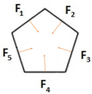
Figure 36: Pentagon with normal vectors

Problem: For any simple $n$-polytope $P$ find all integral $(n\times m)$-matrices

$$\varLambda\;=\;\begin{pmatrix}1&0&\ldots&0&\lambda_{1,n+1}&\ldots&\lambda_{1,m}\\ 0&1&\ldots&0&\lambda_{2,n+1}&\ldots&\lambda_{2,m}\\ \vdots&\vdots&\ddots&\vdots&\vdots&\ddots&\vdots\\ 0&0&\ldots&1&\lambda_{n,n+1}&\ldots&\lambda_{n,m}\end{pmatrix},$$

in which the column $\lambda_{j}=(\lambda_{1,j},\ldots,\lambda_{n,j})$ corresponds to the facet $F_{j},\;j=1,\ldots,m$, and the columns $\lambda_{j_{1}}$, …, $\lambda_{j_{n}}$ corresponding to any vertex$v_{\omega}=F_{j_{1}}\cap\dots\cap F_{j_{n}}$ form a basis for $\mathbb{Z}^{n}$.

Note that there are simple $n$-polytopes, $n\geqslant 4$, admitting no characteristic functions.

Exercise: Let $C^{n}(m)$ be a combinatorial type of a cyclic polytope built as follows: take real numbers $t_{1}<\dots<t_{m}$ and

$$C^{n}(t_{1},\dots,t_{m})={\rm conv}\{(t_{i},t_{i}^{2},\dots,t_{i}^{n}),i=1,\dots,m\}.$$

Prove that

1. the combinatorial type of $C^{n}(t_{1},\dots,t_{m})$ does not depend on $t_{1}<\dots<t_{m}$;

2. the polytope $C^{n}(m)$ is simplicial;

3. for $n\geqslant 4$ any two vertices of $C^{n}(m)$ are connected by an edge;

Conclude that for large $m$ the dual simple polytope $C^{n}(m)^{*}$ admits no characteristic functions.

5 Combinatorial data

Definition 8.3.

The combinatorial quasitoric data $(P,\varLambda)$ consists of an oriented combinatorial simple polytope $P$ and an integer $(n\times m)$-matrix $\varLambda$ with the properties above.

The matrix $\varLambda$ defines an epimorphism

$$\ell\colon\mathbb{T}^{m}\to\mathbb{T}^{n}.$$

The kernel of $\ell$ (which we denote $K(\varLambda)$) is isomorphic to $\mathbb{T}^{m-n}$.

Exercise: The action of $K(\varLambda)$ on $\mathcal{Z}_{P}$ is free due to the condition on the minors of $\varLambda$.

6 Quasitoric manifold with the $(A,\Lambda)$-structure

Construction: The quotient $M=\mathcal{Z}_{P}/K(\varLambda)$ is a $2n$-dimensional smooth manifold with an action of the $n$-dimensional torus $T^{n}=\mathbb{T}^{m}/K(\varLambda)$. We denote this action by $\alpha$. It satisfies the Davis–Januszkiewicz conditions:

1. $\alpha$ is locally isomorphic to the standard coordinatewise representation of $\mathbb{T}^{n}$ in $\mathbb{C}^{n}$,

2. there is a projection $\pi\colon M\to P$ whose fibres are orbits of $\alpha$.

We refer to $M=M(P,\varLambda)$ as the quasitoric manifold associated with the combinatorial data $(P,\varLambda)$.

Let

$$P=\{\boldsymbol{x}\in\mathbb{R}^{n}\colon A\boldsymbol{x}+b\geqslant 0\}.$$

Definition 8.4.

The manifold $M=M(P,\varLambda)$ is called the quasitoric manifold with $(A,\varLambda)$-structure.

Exercise: Suppose the $(n\times m)$-matrix $\varLambda=(I_{n},\,\varLambda_{*})$, where $I_{n}$ is the unit matrix, gives a characteristic mapping

$$\ell\colon\{F_{1},\ldots,F_{m}\}\longrightarrow\mathbb{Z}^{n}$$

Then the matrix $S=\begin{pmatrix}-\varLambda_{*}\\ I_{m-n}\end{pmatrix}$ gives the $(m-n)$-dimensional subgroup

$$H=\bigl{\{}(e^{2\pi i\psi_{1}},\ldots,e^{2\pi i\psi_{m}})\in\mathbb{T}^{m}\bigr{\}},$$

where

$$\psi_{k}=-\sum_{j=n+1}^{m}\lambda_{k,j}\varphi_{j-n},\;k=1,\ldots,n;\;\psi_{k}=\varphi_{k-n},\;k=n+1,\ldots,m,$$

acting freely on $\mathcal{Z}_{P}$.

Example 8.5.

Take $P=\Delta^{2}$. Let us describe the matrices $A$ and $\varLambda$:

$$A=\begin{pmatrix}1&0\\ 0&1\\ a_{31}&a_{32}\end{pmatrix},\qquad\varLambda=\begin{pmatrix}1&0&\lambda_{13}\\ 0&1&\lambda_{23}\end{pmatrix},\qquad a_{31},a_{32},\lambda_{13},\lambda_{23}\in\mathbb{Z}.$$

Since the normal vectors are oriented inside the polytope, $a_{31}<0,\;a_{32}<0$.
Thus, up to combinatorial equivalence, one can take $a_{31}=a_{32}=-1$.
The conditions on the characteristic mapping give

$$\begin{vmatrix}0&\lambda_{13}\\ 1&\lambda_{23}\end{vmatrix}=\pm\,1,\quad\begin{vmatrix}1&\lambda_{13}\\ 0&\lambda_{23}\end{vmatrix}=\pm\,1,\quad\Rightarrow\quad\lambda_{13}=\pm\,1,\quad\lambda_{23}=\pm\,1.$$

Therefore we have 4 structures $(A,\varLambda)$.

Exercise: Let $P=\Delta^{2}$ and $\mathbb{C}P^{2}$ be the complex projective space with
the canonical action of torus $\mathbb{T}^{3}$: $(t_{1},t_{2},t_{3})(z_{1}:z_{2}:z_{3})=(t_{1}z_{1}:t_{2}z_{2}:t_{3}z_{3})$.

1. describe $\mathbb{C}P^{2}$ as $(S^{5}\times_{\mathbb{T}^{3}}\mathbb{T}^{2})$;

2. describe the structure $(A,\varLambda)$ such that $M(A,\varLambda)$ is $\mathbb{C}P^{2}$;

7 A partition of a quasitoric manifold

We have the homeomorphism

$$\mathcal{Z}_{P}\simeq\bigcup_{v_{\omega}-\text{ vertex}}{\mathcal{Z}_{P,v_{\omega}}},$$

where

$$\mathcal{Z}_{P,v_{\omega}}=\prod_{j\in\omega}D^{2}_{j}\times\prod_{j\in[m]\setminus\omega}S^{1}_{j}\subset\mathbb{D}^{2m}.$$

Exercise: $\mathcal{Z}_{P,v_{\omega}}/K(\varLambda)\simeq\mathbb{D}^{2n}_{\omega}$.

Corollary 8.6.

We have the partition:

$$M(P,\varLambda)=\bigcup_{v_{\omega}-\text{ vertex}}\mathbb{D}^{2n}_{\omega}.$$

8 Stably complex structure and characteristic classes

Denote by $\mathbb{C}_{i}$ the space of the 1-dimensional complex representation of the torus $\mathbb{T}^{m}$ induced from the standard representation in $\mathbb{C}^{m}$ by the projection $\mathbb{C}^{m}\to\mathbb{C}_{i}$ onto the $i$th coordinate. Let $\mathcal{Z}_{P}\times\mathbb{C}_{i}\to\mathcal{Z}_{P}$ be the trivial complex line bundle; we view it as an equivariant $\mathbb{T}^{m}$-bundle with the diagonal action of $\mathbb{T}^{m}$. By taking the quotient with respect to the diagonal action of $K=K(\varLambda)$ we obtain a $T^{n}$-equivariant complex line bundle

$$\rho_{i}\colon\mathcal{Z}_{P}\times_{K}\mathbb{C}_{i}\to\mathcal{Z}_{P}/K=M(P,\varLambda)$$ (3)

over the quasitoric manifold $M=M(P,\varLambda)$. Here

$$\mathcal{Z}_{P}\times_{K}\mathbb{C}_{i}=\mathcal{Z}_{P}\times\mathbb{C}_{i}\left/\right.(\boldsymbol{t}\boldsymbol{z},\boldsymbol{t}w)\sim(\boldsymbol{z},w)\text{ for any }\boldsymbol{t}\in K,\boldsymbol{z}\in\mathcal{Z}_{P},w\in\mathbb{C}_{i}.$$

Theorem 8.7.

(Theorem 6.6, [15]) There is an isomorphism of real $T^{n}$-bundles over $M=M(P,\varLambda)$:

$${\mathcal{T}}\!M\oplus\underline{\mathbb{R}}^{2(m-n)}\cong\rho_{1}\oplus\cdots\oplus\rho_{m};$$ (4)

here $\underline{\mathbb{R}}^{2(m-n)}$ denotes the trivial real $2(m-n)$-dimensional $T^{n}$-bundle over $M$.

For the proof see (Theorem 7.3.15, [7]) .

Corollary 8.8.

Let $v_{i}=c_{1}(\rho_{i})\in H^{2}(M(P,\Lambda),\mathbb{Z})$. Then for the total Chern class we have

$$C(M(P,\Lambda))=1+c_{1}+\dots+c_{n}=(1+v_{1})\dots(1+v_{m}),$$

and for the total Pontryagin class we have

$$P(M(P,\Lambda))=1+p_{1}+\dots+p_{\left[\frac{n}{2}\right]}=(1+v_{1}^{2})\dots(1+v_{m}^{2}).$$

9 Cohomology ring of the quasitoric manifold

Theorem 8.9.

[15] We have

$$H^{*}(M(P,\Lambda))=\mathbb{Z}[v_{1},\dots,v_{m}]/(J_{SR}(P)+I_{P,\Lambda}),$$

where $v_{i}=c_{1}(\rho_{i})$, $J_{SR}(P)$ is the Stanley-Reisner ideal generated by monomials $\{v_{i_{1}}\dots v_{i_{k}}\colon F_{i_{1}}\cap\dots\cap F_{i_{k}}=\varnothing\}$, and $I_{P,\Lambda}$ is the ideal generated by the linear forms $\lambda_{i,1}v_{1}+\dots+\lambda_{i,m}v_{m}$ arising from the equality

$$\ell(F_{1})v_{1}+\dots+\ell(F_{m})v_{m}=0.$$

For the proof see (Theorem 7.3.28, [7]).

Corollary 8.10.

If $\Lambda=(I_{n},\Lambda_{*})$, then

$$H^{2}(M(P,\Lambda))=\mathbb{Z}^{m-n}$$

with the generators $v_{n+1},\dots,v_{m}$.

Corollary 8.11.

1. The group $H^{k}(M(P,\Lambda))$ is nontrivial only for $k$ even;

2. $M(P,\Lambda)$ is even dimensional and orientable, hence the group $H_{k}(M(P,\Lambda))$ is nontrivial only for $k$ even;

3. from the universal coefficients formula the abelian groups $H^{*}(M(P,\Lambda))$ and $H_{*}(M(P,\Lambda))$ have no torsion.

Corollary 8.12.

Let $P$ be a flag polytope and $\ell$ be its characteristic function. Then

$$H^{*}(M(P,\Lambda))=\mathbb{Z}[v_{1},\dots,v_{m}]/(J_{SR}+I_{P,\Lambda}),$$

where the ideal $J_{SR}$ is generated by monomials $v_{i}v_{j}$, where $F_{i}\cap F_{j}=\varnothing$, and $I_{P,\Lambda}$ is generated by linear forms $\lambda_{i,1}v_{1}+\dots+\lambda_{i,m}v_{m}$.

Corollary 8.13.

For any $l=1,\dots,n$, the cohomology group $H^{2l}(M(P,\Lambda),\mathbb{Z})$ is generated by monomials $v_{i_{1}}\dots v_{i_{l}}$, $i_{1}<\dots<i_{l}$, corresponding to $(n-l)$-faces $F_{i_{1}}\cap\dots\cap F_{i_{l}}$.

Proof 8.14.

We will prove this by induction on characteristic $\delta=\sum_{p_{i}>1}p_{i}$ of a monomial $v_{i_{1}}^{p_{1}}\dots v_{i_{s}}^{p_{s}}$ with $i_{1}<\dots<i_{s}$. Due to the relations from the ideal $J_{SR}$ nonzero monomials correspond to faces $F_{i_{1}}\cap\dots\cap F_{i_{s}}\neq\varnothing$. If $\delta=0$, then we have the monomial we need. If $\delta>0$, then take a vertex $v$ in $F_{i_{1}}\cap\dots\cap F_{i_{s}}\neq\varnothing$. Let $\Lambda_{v}$ be the submatrix of $\Lambda$ corresponding to the columns $\{j\colon v\in F_{j}\}$. Then by definition of a characteristic function $\det\Lambda_{v}=\pm 1$. By integer elementary transformations of rows of the matrix $\Lambda$ (hence of linear relations in the ideal $I_{P,\Lambda}$) we can make $\Lambda_{v}=E$. Let $p_{k}>1$. The variable $v_{i_{k}}$ can be expressed as a linear combination $v_{i_{k}}=\sum\limits_{j\notin\{i_{1},\dots,i_{s}\}}a_{j}v_{j}$. Then

$$v_{i_{1}}^{p_{1}}\dots v_{i_{s}}^{p_{s}}=\sum\limits_{j\notin\{i_{1},\dots,i_{s}\}}a_{j}v_{i_{1}}^{p_{1}}\dots v_{i_{k}}^{p_{k}-1}\dots v_{i_{s}}^{p_{s}}v_{j},$$

where on the right side we have the sum of monomials with less value of $\delta$. This finishes the proof.

For any $\xi=(i_{1},\ldots,i_{n-1})\subset[m]$ set $\xi_{i}=(\xi,i),\;i\notin\xi$.

Exercise:
1. For any $\xi=(i_{1},\ldots,i_{n-1})\subset[m]$ there are the relations

$$\sum_{j=1}^{m}\varepsilon(\xi_{j})v_{j}=0$$ (5)

where $\varepsilon(\xi_{j})=\det|\ell(F_{i_{1}}),\ldots,\ell(F_{i_{n-1}}),\ell(F_{j})|$.
2. There is a graded ring isomorphism

$$H^{*}(M(P,\Lambda))=\mathbb{Z}[P]/J$$

where $J$ is the ideal generated by the relations (5).

Exercise: For any vertex $v_{\omega}=F_{i_{1}}\bigcap\dots\bigcap F_{i_{n}},\;\omega=(i_{1},\ldots,i_{n})$, there are the relations

$$v_{i_{n}}=-\varepsilon(\xi_{i_{n}})\sum_{j}\varepsilon(\xi_{j})\,v_{j}$$

where $\xi=(i_{1},\ldots,i_{n-1}),\;j\in[m\backslash\xi_{i_{n}}]$.

Exercise: For any vertex $v_{\omega}=F_{i_{1}}\bigcap\dots\bigcap F_{i_{n}},\;\omega=(i_{1},\ldots,i_{n})$, there are the relations

$$v_{i_{n}}^{2}=-\varepsilon(\xi_{i_{n}})\sum_{j}\varepsilon(\xi_{j})\,v_{i_{n}}v_{j}$$

where $j\in[m\backslash\xi_{i_{n}}]$, but $F_{i_{n}}\bigcap F_{j}\neq\emptyset$.

10 Geometrical realization of cycles of quasitoric manifolds

The fundamental notions of algebraic topology were introduced in the classical work by Poincare [37]. Among them there were notions of cycles and homology. Quasitoric manifolds give nice examples of manifolds such that original notions by Poincare obtain explicit geometric realization.

Let $M^{k}$ be a smooth oriented manifold such that the groups $H_{*}(M^{k},\mathbb{Z})$ have no torsion. There is the classical Poincare duality $H_{i}(M^{k},\mathbb{Z})\simeq H^{k-i}(M^{k},\mathbb{Z})$. Moreover, according to the Milnor-Novikov theorem [34, 35, 36] for any cycle $a\in H_{l}(M^{k},\mathbb{Z})$ there is a smooth oriented manifold $N^{l}$ and a continuous mapping $f\colon N^{l}\to M^{k}$ such that $f_{*}[N^{l}]=a$. For the homology groups of any quasitoric manifold there is the following remarkable geometrical interpretation of this result. Note that odd homology groups of any quasitoric manifold are trivial.

Theorem 8.15.

1. The homology group $H_{2n-2}(M(P,\Lambda),\mathbb{Z})$ of the quasitoric manifold $M^{2n}(P,\Lambda)$ is generated by embedded quasitoric manifolds $M^{2n-2}_{i}(P,\Lambda)$, $i=1,\dots,m$, of facets of $P$. The embedding of the manifold $M^{2n-2}_{i}(P,\Lambda)\subset M(P,\Lambda)$ gives the geometric realization of the cycle Poincare dual to the cohomology class $v_{i}\in H^{2}(M(P,\Lambda),\mathbb{Z})$ defined above.

2. For any $i$ the homology group $H_{2i}(M(P,\Lambda),\mathbb{Z})$ is generated by embedded quasitoric manifolds corresponding to all $i$-faces $F_{j_{1}}\cap\dots\cap F_{j_{n-i}}$ of the polytope $P$. These manifolds can be described as complete intersections of manifolds $M^{2n-2}_{j_{1}}(P,\Lambda)$, $\dots$, $M^{2n-2}_{j_{n-i}}(P,\Lambda)$.

The proof of the theorem follows directly from the above results on the cohomology of quasitoric manifolds and geometric interpretation of the Poincare duality in terms of Thom spaces [42].

11 Four colors problem

Classical formulation: Given any partition of a plane into contiguous regions, producing a figure called a map, two regions are called adjacent if they share a common boundary that is not a corner, where corners are the points shared by three or more regions.

Problem: No more than four colors are required to color the regions of the map so that no two adjacent regions have the same color.

The problem was first proposed on October 23, 1852, when Francis Guthrie, while trying to color the map of counties of England, noticed that only four different colors were needed.

The four colors problem became well-known in 1878 as a hard problem when Arthur Cayley suggested it for discussion during the meeting of the London mathematical society.

The four colors problem was solved in 1976 by Kenneth Appel and Wolfgang Haken. It became the first major problem solved using a computer. For the details and the history of the problem see [45]. One of the central topics of this monograph is <<how the problem was solved>>.

Example 8.16.

Platonic solids.
The octahedron can be colored in $2$ colors.
The cube and the icosahedron can be colored into $3$ colors.
The tetrahedron and the dodecahedron can be colored into $4$ colors.

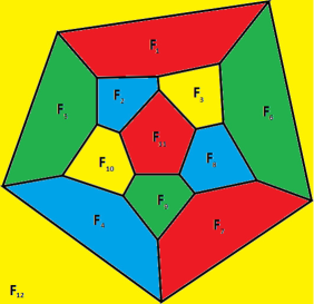
Figure 37: Coloring of the dodecahedron

Exercise: Color all the Archimedean solids.

12 Quasitoric manifolds of $3$-dimensional polytopes

Let $P$ be a simple $3$-polytope. Then $\partial P$ is homeomorphic to the sphere $S^{2}$ partitioned into polygons $F_{1},\dots,F_{m}$. By the four colors theorem there is a coloring $\varphi\colon\{F_{1},\dots,F_{m}\}\to\{1,2,3,4\}$ such that adjacent facets have different colors.

Let $\boldsymbol{e}_{1},\boldsymbol{e}_{2},\boldsymbol{e}_{3}$ be the standard basis for $\mathbb{Z}^{3}$, and $\boldsymbol{e}_{4}=\boldsymbol{e}_{1}+\boldsymbol{e}_{2}+\boldsymbol{e}_{3}$.

Proposition 8.17.

The mapping $\ell\colon\{F_{1},\dots,F_{m}\}\to\mathbb{Z}^{3}\colon\ell(F_{i})=\boldsymbol{e}_{\varphi(F_{i})}$ is a characteristic function.

Corollary 8.18.

• Any simple $3$-polytope $P$ has combinatorial data $(P,\Lambda)$ and the quasitoric manifold $M(P,\Lambda)$;

• Any fullerene has a quasitoric manifold.

Since a fullerene is a flag polytope, the cohomology ring of any its quasitoric manifold is described by Corollary 8.12.

Exercise: Find a $4$-coloring of the barrel (Fig. 38).

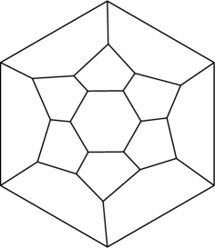
Figure 38: Schlegel diagram of the barrel

9 Lecture 9. Construction of fullerenes

1 Number of combinatorial types of fullerenes

Definition 9.1.

Two combinatorially nonequivalent fullerenes with the same number $p_{6}$ are called combinatorial isomers.

Let $F(p_{6})$ be the number of combinatorial isomers with given $p_{6}$.

From the results by W. Thurston [43] it follows that $F(p_{6})$ grows like $p_{6}^{9}$.

There is an effective algorithm of combinatorial enumeration of fullerenes using supercomputer (Brinkmann-Dress [3], 1997). It gives:

$p_{6}$	0	1	2	3	4	5	6	7	8	$\dots$	75
$F(p_{6})$	1	0	1	1	2	3	6	6	15	$\dots$	46.088.157

We see that for large value of $p_{6}$ the number of combinatorial isomers is very huge. Hence there is an important problem to study different structures on the set of fullerenes.

2 Growth operations

The well-known problem [2, 28] is to find a simple set of operations sufficient to construct arbitrary fullerene from the dodecahedron.

Definition 9.2.

A patch is a disk bounded by a simple edge-cycle on the boundary of a simple $3$-polytope.

Definition 9.3.

A growth operation is a combinatorial operation that gives a new $3$-polytope $Q$ from a simple $3$-polytope $P$ by substituting a new patch with the same boundary and more facets for the patch on the boundary of $P$.

The Endo-Kroto operation [21] (Fig. 39) is the simplest example of a growth operation that changes a fullerene into a fullerene.

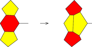
Figure 39: Endo-Kroto operation

It was proved in [2] that there is no finite set of growth operations transforming fullerenes into fullerenes sufficient to construct arbitrary fullerene from the dodecahedron. In [28] the example of an infinite set was found. Our main result is the following (see [10]): if we allow at intermediate steps polytopes with at most one singular face (a quadrangle or a heptagon), then only $9$ growth operations (induced by $7$ truncations) are sufficient.

Exercise: Starting from the Barrel fullerene (see Fig. 38) using the Endo-Kroto operation construct a fullerene with arbitrary $p_{6}\geqslant 2$.

3 $(s,k)$-truncations

First we mention a well-known result about construction of simple $3$-polytopes.

Theorem 9.4.

(Eberhard (1891), Brückner (1900)) A $3$-polytope is simple if and only if it is combinatorially equivalent to a polytope obtained from the tetrahedron by a sequence of vertex, edge and $(2,k)$-truncations.

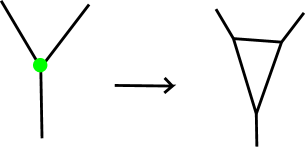
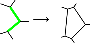
Figure 40: Vertex-, edge- and $(2,k)$-truncations

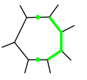
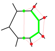
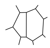
Figure 41: $(3,7)$-truncation

Construction ($(s,k)$-truncation): Let $F_{i}$ be a $k$-gonal face of a simple $3$-polytope $P$.

choose $s$ consequent edges of $F_{i}$;

rotate the supporting hyperplane of $F_{i}$ around the axis passing through the midpoints of adjacent two edges (one on each side);

take the corresponding hyperplane truncation. We call it $(s,k)$-truncation .

Example 9.5.

1. Vertex truncation is a $(0,k)$-truncation.

2. Edge truncation is a $(1,k)$-truncation.

3. The Endo-Kroto operation is a $(2,6)$-truncation.

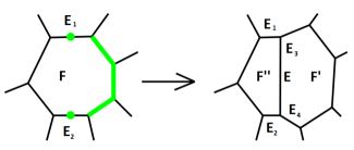
Figure 42: $(s,k)$-truncation

The next result follows from definitions.

Proposition 9.6.

Under the $(s,k)$-truncation of the polytope $P$ its facets that do not contain the edges $E_{1}$ and $E_{2}$ (see Fig. 42) preserve the number of sides.

The facet $F$ is split into two facets: an $(s+3)$-gonal facet $F^{\prime}$ and a $(k-s+1)$-gonal facet $F^{\prime\prime}$, $F^{\prime}\cap F^{\prime\prime}=E$.

The number of sides of each of the two facets adjacent to $F$ along the edges $E_{1}$ and $E_{2}$ increases by one.

Remark 9.7.

We see that $(s,k)$-truncation is a combinatorial operation and is always defined. It is easy to show that the straightening along the edge $E$ on the right side is a combinatorially inverse operation. It is not always defined.

Definition 9.8.

If the facets intersecting $F$ by $E_{1}$ and $E_{2}$ (see Fig. 42) are $m_{1}$- and $m_{2}$-gons respectively, then we also call the corresponding operation an $(s,k;m_{1},m_{2})$-truncation.

For $s=1$ combinatorially $(1,k;m_{1},m_{2})$-truncation is the same operation as $(1,t;m_{1},m_{2})$-truncation of the same edge of the other facet containing it. We call this operation simply a $(1;m_{1},m_{2})$-truncation.

Remark 9.9.

Let $P$ be a flag simple polytope. Then any $(s,k)$-truncation is a growth operation. Indeed, for $s=0$ and $s=k-2$ we have the vertex truncation, which can be considered as the substitution of the corresponding fragment for the three facets containing the vertex. For $0<s<k-2$, since $P$ is flag, the facets $F_{i_{1}}$ and $F_{i_{s+2}}$ intersecting $F$ by edges adjacent to truncated edges do not intersect; hence the union $F_{i_{1}}\cup F\cup F_{i_{s+2}}$ is bounded by a simple edge-cycle (see Fig. 43 on the left). After the $(s,k)$-truncation the union of facets $F^{\prime}\cup F^{\prime\prime}\cup F_{i_{1}}\cup F_{i_{s+2}}$ is bounded by combinatorially the same simple edge-cycle. We describe this operation by the scheme on Fig. 43 on the right.

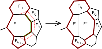
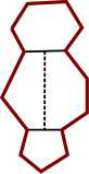
Figure 43: $(s,k)$-truncation as a growth operation

For $s=1$ as mentioned above the edge-truncation can be considered as a $(1,k)$-truncation and a $(1,t)$-truncation for two facets containing the truncated edge: an $s$-gon and a $t$-gon. This gives two different patches, which differ by one facet.

Exercise: Consider the set of $k-s-2$ edges of the face $F$ that are not adjacent to the $s$ edges defining the $(s,k)$-truncation. The polytope $Q^{\prime}$ obtained by the $(k-s-2,k)$-truncation along these edges is combinatorially equivalent to the polytope $Q$. In particular

The $(k-3,k)$-truncation is combinatorially equivalent to the edge truncation;

The $(k-2,k)$-truncation is combinatorially equivalent to the vertex truncation.

Exercise: Let $P$ be a flag $3$-polytope. Then the polytope obtained from $P$ by an $(s,k)$-truncation is flag if and only if $0<s<k-2$.

In [9] the analog of Theorem 9.4 for flag polytopes was proved.

Theorem 9.10.

A simple $3$-polytope is flag if and only if it is combinatorially equivalent to a polytope obtained from the cube by a sequence of edge truncations and $(2,k)$-truncations, $k\geqslant 6$.

4 Construction of fullerenes by truncations

Definition 9.11.

Let $\mathfrak{F}_{-1}$ be the set of combinatorial simple polytopes with all facets pentagons and hexagons except for one singular facet quadrangle.

Let $\mathfrak{F}$ be the set of all fullerenes.

Let $\mathfrak{F}_{1}$ be the set of simple polytopes with one singular facet heptagon adjacent to a pentagon such that either there are two pentagons with the common edge intersecting the heptagon and a hexagon (we will denote this fragment $F_{5567}$, see Fig. 44), or for any two adjacent pentagons exactly one of them is adjacent to the heptagon.

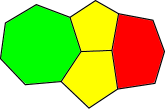
Figure 44: Fragment $F_{5567}$

Set $\mathfrak{F}_{s}=\mathfrak{F}_{-1}\sqcup\mathfrak{F}\sqcup\mathfrak{F}_{1}$ to be se set of singular fullerenes

Theorem 9.12.

Any polytope in $\mathfrak{F}_{s}$ can be obtained from the dodecahedron by a sequence of $p_{6}$ truncations: $(1;4,5)$-, $(1;5,5)$-, $(2,6;4,5)$-, $(2,6;5,5)$-, $(2,6;5,6)$-, $(2,7;5,5)$-, and $(2,7;5,6)$-, in such a way that intermediate polytopes belong to $\mathfrak{F}_{s}$.

More precisely:

1. any polytope in $\mathfrak{F}_{-1}$ can be obtained by a $(1;5,5)$- or $(1;4,5)$-truncation from a fullerene or a polytope in $\mathfrak{F}_{-1}$ respectively;

2. any polytope in $\mathfrak{F}_{1}$ can be obtained by a $(2,6;5,6)$- or $(2,7;5,6)$-truncation from a fullerene or a polytope in $\mathfrak{F}_{1}$ respectively;

3. any fullerene can be obtained by a $(2,6;5,5)$-, $(2,6;4,5)$-, or $(2,7;5,5)$-truncation from a fullerene or a polytope from $\mathfrak{F}_{-1}$ or $\mathfrak{F}_{1}$ respectively.

Figure 45: Scheme of the truncation operations

Proof 9.13.

By Theorems 3.13 and 3.19 any polytope in $\mathfrak{F}_{s}$ has no $3$-belts and the only possible $4$-belt surrounds a quadrangular facet. Hence for any edge the operation of straightening is well-defined.

For (1) we need the following result.

Lemma 9.14.

There is no polytopes in $\mathfrak{F}_{-1}$ with the quadrangle surrounded by pentagons.

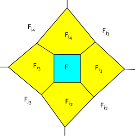
Figure 46: Quadrangle surrounded by pentagons

Proof 9.15.

Let the quadrangle $F$ be surrounded by pentagons $F_{i_{1}}$, $F_{i_{2}}$,$F_{i_{3}}$, and $F_{i_{4}}$ as drawn on Fig. 46. By Theorem 3.19 we have the $4$-belt $\mathcal{B}=(F_{i_{1}},F_{i_{2}},F_{i_{3}},F_{i_{4}})$ surrounding $F$, and there are no other $4$-belts. Let $\mathcal{L}=(F_{j_{1}},F_{j_{2}},F_{j_{3}},F_{j_{4}})$ be a $4$-loop that borders $\mathcal{B}$ along its boundary component different from $\partial F$. Its consequent facets are different. If $F_{j_{1}}=F_{j_{3}}$, then we obtain a $4$-belt $(F,F_{i_{1}},F_{j_{1}},F_{i_{3}})$, which is a contradiction. Similarly $F_{j_{2}}\neq F_{j_{4}}$. Hence $\mathcal{L}$ is a simple $4$-loop. Since it is not a $4$-belt its two opposite facets intersect, say $F_{j_{1}}\cap F_{j_{3}}\neq\varnothing$. Then $F_{j_{1}}\cap F_{j_{2}}\cap F_{j_{3}}$ is a vertex and $F_{j_{2}}$ is a quadrangle. A contradiction. This proves the lemma.

Thus, for any polytope $P$ in $\mathfrak{F}_{-1}$ its quadrangle $F$ is adjacent to some hexagon $F_{i}$ by some edge $E$. Now straighten the polytope $P$ along the edge of $F$ adjacent to $E$ to obtain a new polytope $Q$ with a pentagon instead of $F_{i}$ and a pentagon or a quadrangle instead of the facet $F_{j}$ adjacent to $F$ by the edge of $F$ opposite to $E$. In the first case $Q$ is a fullerene and $P$ is obtained from $Q$ by a $(1;5,5)$-truncation. In the second case $Q\in\mathfrak{F}_{-1}$ and $P$ is obtained from $Q$ by a $(1;4,5)$-truncation. This proves (1).

To prove (2) note that if $P\in\mathfrak{F}_{1}$ contains the fragment $F_{5567}$, then straightening along the common edge of pentagons gives a fullerene $Q$ such that $P$ is obtained from $Q$ by a $(2,6;5,6)$-truncation.

Lemma 9.16.

If $P\in\mathfrak{F}_{1}$ does not contain the fragment $F_{5567}$, then

1. $P$ does not contain fragments on Fig. 47;

2. for any pair of adjacent pentagons any of them does not intersect any other pentagons.

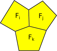
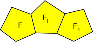
Figure 47: Fragments that can not be present on the polytope in $\mathfrak{F}_{1}$ without the fragment $F_{5567}$

Proof 9.17.

Let $F_{i}$, $F_{j}$, $F_{k}$ be pentagons with a common vertex. Then for the pair $(F_{i},F_{j})$ exactly one pentagon intersects the heptagon $F$, say $F_{i}$. Also for the pair $(F_{j},F_{k})$ exactly one pentagon intersects $F$. This should be $F_{k}$. For the pair $(F_{i},F_{k})$ this is a contradiction.

Let the pentagon $F_{j}$ intersects pentagons $F_{i}$ and $F_{k}$ by non-adjacent edges as shown in Fig. 47 on the right. The heptagon $F$ should intersect exactly one pentagon of each pair $(F_{i},F_{j})$ and $(F_{j},F_{k})$. Then either it intersects $F_{i}$ and $F_{k}$ and does not intersect $F_{j}$, or it intersects $F_{j}$ and does not intersect $F_{i}$ and $F_{k}$. By Theorem 3.13 $P$ has no $3$-belts; hence $F_{i}\cap F_{k}=\varnothing$. In the first case we obtain the $4$-belt $(F,F_{i},F_{j},F_{k})$, which contradicts Theorem 3.19. In the second case $F$ intersects $F_{j}$ by one of the three edges different from $F_{i}\cap F_{j}$ and $F_{j}\cap F_{k}$. But any of these edges intersects either $F_{i}$, or $F_{k}$, which is a contradiction.

Thus we have proved part (1) of the lemma. Let some pentagon of the pair of adjacent pentagons $(F_{i},F_{j})$, say $F_{j}$, intersects some other pentagon $F_{k}$. If the edges of intersection are adjacent in $F_{j}$, then we obtain the fragment on Fig. 47 on the left. Else we obtain the fragment on Fig. 47 on the right. A contradiction. This proves part (2) of the lemma.

Now assume that $P$ does not contain the fragment $F_{5567}$.

Let $(F_{i},F_{j})$ be a pair of two adjacent pentagons with $F_{i}$ intersecting the heptagon $F$. Then by Lemma 9.16 we obtain the fragment on Fig. 48 a). Since by Proposition 2.8 the pair of adjacent facets is surrounded by a belt, the adjacent pentagons do not intersect other pentagons and exactly one of them intersects the heptagon. The straightening along the edge $F_{i}\cap F_{p}$ gives a polytope $Q$ such that $P$ is obtained from $Q$ by a $(2,7;5,6)$-truncation. $Q$ has all facets pentagons and hexagons except for one heptagon adjacent to a pentagon. $Q$ contains the fragment $F_{5567}$; hence it belongs to $\mathfrak{F}_{1}$.

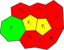
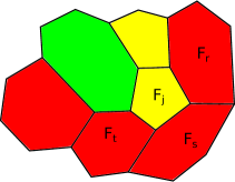
a)	b)

Figure 48: a) facets surrounding the pair of adjacent pentagons; b) the same fragment after the straightening

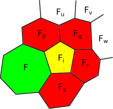
a)	b)

Figure 49: a) facets surrounding a pentagon adjacent to the heptagon; b) the same fragment after the straightening

Now let $P$ have no adjacent pentagons. Consider a pentagon adjacent to the heptagon $F$. Then it is surrounded by a $5$-belt $\mathcal{B}$ consisting of the heptagon and $4$ hexagons (Fig. 49 a). The straightening along the edge $F_{p}\cap F_{i}$ gives a simple polytope $Q$ with the fragment on Fig. 49 b) instead the fragment on Fig. 49 a). The polytope $Q$ has all facets pentagons and hexagons except for one heptagon $F_{p,i}$ adjacent to the pentagon $F_{q}$. Then $P$ is obtained from $Q$ by a $(2,7;5,6)$-truncation. We claim that $Q\in\mathfrak{F}_{1}$. Indeed, if $Q$ has the fragment $F_{5567}$, it is true. If $Q$ has no such fragments consider two adjacent pentagons of $Q$. The polytopes $P$ and $Q$ have the same structure outside the fragments in consideration; hence $Q$ has the same pentagons as $P$ except for $F_{q}$, which appeared instead of $F_{i}$. Also $P$ has all pentagons isolated; hence one of the adjacent pentagons is $F_{q}$. The second pentagon $F_{t}$ should be adjacent to the hexagon $F_{q}$ in $P$; hence it should be one of the facets $F_{u}$, $F_{v}$, or $F_{w}$ on Fig. 49 a). Each of these facets is different from $F$, since they lie outside the $5$-belt $\mathcal{B}$ containing $F$. And in each case the pentagon $F_{t}$ is isolated in $P$ by assumption.

If $F_{t}=F_{u}$, then $F_{v}$ is a hexagon, since $F_{v}\neq F$ and $F_{v}$ is not a pentagon. Then $Q$ contains the fragment $F_{5567}$, which is a contradiction. Thus $F_{u}$ is a hexagon.

If $F_{t}$ is one of the facets $F_{v}$ and $F_{w}$, then the other facet is a hexagon and there are no pairs of adjacent pentagons in $Q$ other than $(F_{q},F_{t})$. Each of the facets $F_{v}$, $F_{w}$ in $Q$ belongs to the $5$-belt surrounding $F_{q}$ together with $F_{p,i}$ and is not successive with it; hence $F_{v}$ and $F_{w}$ do not intersect $F_{p,i}$ in $Q$. Thus $F_{t}\cap F_{p,i}=\varnothing$ and $Q\in\mathfrak{F}_{1}$. This proves (2).

To prove (3) consider a fullerene $P$. If it contains the fragment on Fig. 50 a) then the straightening along the edge $F_{i}\cap F_{j}$ gives a fullerene $Q$ such that $P$ is obtained from $Q$ by a $(2,6;5,5)$-truncation (the Endo-Kroto operation). Let $P$ contain no such fragments.

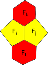
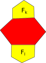
a)	b)

Figure 50: a) Two adjacent pentagons with two hexagons; b) the same fragment after the straightening

If $P$ has two adjacent pentagons, then one of the connected components of unions of pentagons has more than two pentagons. If $P$ is not combinatorially equivalent to the dodecahedron, then each component is a sphere with holes. Consider the connected component with more than one pentagon and a vertex $v$ on its boundary lying in two pentagons $F_{i}$ and $F_{j}$. Then the third face containing $v$ is a hexagon. Since $P$ contains no fragments on Fig. 50 a), the other facet intersecting the edge $F_{i}\cap F_{j}$ by the vertex is a pentagon and we obtain the fragment on Fig. 51 a). Then the straightening along the edge $F_{i}\cap F_{j}$ gives the polytope $Q\in\mathfrak{F}_{-1}$ such that $P$ is obtained from $Q$ by a $(2,6;4,5)$-truncation.

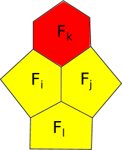
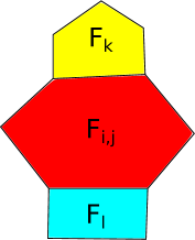
a)	b)

Figure 51: a) Three adjacent pentagons and a hexagon; b) the same fragment after the straightening

If $P$ has no adjacent pentagons, then consider the pentagon $F_{i}$ adjacent to a hexagon $F_{j}$. The straightening along the edge $F_{i}\cap F_{j}$ gives the polytope $Q$ with all facets pentagons and hexagons except for one heptagon $F_{i,j}$ adjacent to a pentagon. $P$ is obtained from $Q$ by a $(2,7;5,5)$-truncation. We claim that $Q\in\mathfrak{F}_{1}$. Indeed, if $Q$ contains the fragment $F_{5567}$, then it is true. Else consider two adjacent pentagons in $Q$. The polytopes $P$ and $Q$ have the same structure outside the fragments on Fig 52; hence $Q$ has the same pentagons as $P$ except for pentagons $F_{k}$ and $F_{l}$, which appeared instead of $F_{i}$. Also $P$ has all pentagons isolated; hence one of the adjacent pentagons is $F_{k}$ or $F_{l}$. We have $F_{k}\cap F_{l}=\varnothing$, else $(F_{k},F_{l},F_{i,j})$ is a $3$-belt. Hence the other adjacent pentagon $F_{t}$ does not belong to $\{F_{k},F_{l}\}$. If $F_{t}$ is adjacent to the heptagon $F_{i,j}$, then in $P$ it is adjacent to $F_{i}$ or $F_{j}$. Since $F_{i}$ is an isolated pentagon, this is impossible. Hence $F_{t}$ should be adjacent to $F_{j}$. Then $F_{t}$ is one of the facets $F_{u}$, $F_{v}$, $F_{w}$ on Fig. 52. Let $F_{t}=F_{u}$. Since $F_{u}$ is an isolated pentagon in $P$, the facet $F_{p}$ is a hexagon on $P$ and on $Q$, since $F_{p}\neq F_{l}$ because $F_{k}\cap F_{l}=\varnothing$. Then we obtain the fragment $F_{5567}$, which is a contradiction. The same argument works for $F_{w}$ instead of $F_{u}$. If $F_{t}=F_{v}$, then $F_{v}\cap F_{k}\neq\varnothing$, or $F_{v}\cap F_{l}\neq\varnothing$, which is impossible, since this gives the $3$-belts $(F_{k},F_{j},F_{v})$, or $(F_{l},F_{j},F_{v})$. Thus, $F_{t}$ does not intersect the heptagon $F_{i,j}$, and $Q\in\mathfrak{F}_{1}$. This finishes the proof of (3) and of the theorem.

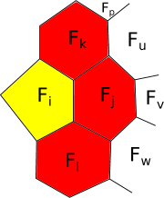
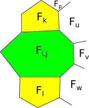
a)	b)

Figure 52: a) Pentagon adjacent to three hexagons; b) the same fragment after the straightening

Remark 9.18.

According to Remark 9.9 the $7$ truncations from Theorem 9.12 give rise to $9$ different growth operations (see Fig. 53):

Each $(1;m_{1},m_{2})$-truncation gives rise to $2$ growth operations:

if the truncated edge belongs to a pentagon, then we have the patch consisting of the pentagon adjacent to an $m_{1}$-gon and an $m_{2}$-gon by non-adjacent edges;

if the truncated edge belongs to two hexagons, then we have the patch consisting of the hexagon adjacent to an $m_{1}$-gon and an $m_{2}$-gon by two edges that are not adjacent and not opposite;

Each of the truncations $(2,6;4,5)$-, $(2,6;5,5)$-, $(2,6;5,6)$-, $(2,7;5,5)$-, and $(2,7;5,6)$- gives rise to one growth operation.

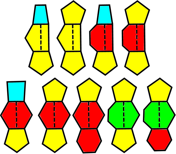
Figure 53: $9$ growth operations induced by $7$ truncations

If we take care of the orientation, then $3$ of the operations have left and right versions.

Acknowledgments

The content of this lecture notes is based on lectures given by the first author at IMS of National University of Singapore in August 2015 during the Program on Combinatorial and Toric Homotopy, and the work originated from the second authors participation in this Program. The authors thank Professor Jelena Grbic (University of Southampton), Professor Jie Wu (National University of Singapore), and IMS for organizing the Program and providing such a nice opportunity.

This work was partially supported by the RFBR grants 14-01-00537 and 16-51-55017, and the Young Russian Mathematics award.

References

- [1] L.J. Billera, C.W. Lee, “A proof of sufficiency of McMullen’s conditions for -vectors of simplicial polytopes”, J. Combin. Theory Ser. A, 31:3 (1981), pp. 237–255.
-
[2]
G.Brinkmann , J.E. Graver, C. Justus, “Numbers of faces in disordered patches”,
J. Math. Chem. 45:2 (2009), pp. 263–278. - [3] G. Brinkmann, A.W.M. Dress, “A constructive enumeration of fullerenes,” J. Algorithms 23 (2), 1997, pp. 345–358.
- [4] W. Bruns, J. Gubeladze, “Polytopes, Rings, and -Theory”, Springer, 2009.
- [5] V.M. Buchstaber and T.E. Panov, “Torus actions and their applications in topology and combinatorics,” AMS University Lectures Series 24, American Mathematical Society, Providence, RI, 2002.
- [6] Victor Buchstaber, “Toric Topology of Stasheff Polytopes,” MIMS EPrint: 2007.232.
- [7] V.M. Buchstaber, T.E. Panov, “Toric Topology,” AMS Math. Surveys and monographs, vol. 204, 2015. 518 pp.
- [8] V.M. Buchstaber, N. Ray “An invitation to toric topology: vertex four of a remarkable tetrahedron”, In Toric topology, M. Harada et al., eds. Contemp. Math., 460, Amer. Math. Soc., Providence, RI, 2008, pp. 1–27.
- [9] V.M. Buchstaber, N. Erokhovets, “Graph-truncations of simple polytopes”, Proc. of Steklov Math Inst, MAIK, Moscow, vol. 289, 2015, pp. 104–133.
- [10] V.M. Buchstaber, N.Yu. Erokhovets, “Construction of fullerenes”, arXiv 1510.02948, 2015.
- [11] V.M. Buchstaber, T.E. Panov, “Algebraic topology of manifolds defined by simple polytopes”, Russian Mathematical Surveys, 1998, 53:3, pp. 623–625.
- [12] V.M. Buchstaber, T.E. Panov, N. Ray, “Spaces of polytopes and cobordism of quasitoric manifolds", Mosc. Math. J., 7:2 (2007), 219–242 , arXiv 0609346.
- [13] H.S.M. Coxeter, “Regular Polytopes”, (3rd edition, 1973), Dover edition, ISBN 0-486-61480-8.
-
[14]
R.F. Curl, “Dawn of the Fullerenes: Experiment and
Conjecture”, Nobel Lecture,
December 7, 1996. - [15] M.Davis, T.Januszkiewicz, “Convex polytopes, Coxeter orbifolds and torus actions", Duke Math. J., 1991. V.62, N2, pp. 417–451.
- [16] M. Deza, M.Dutour Sikiric, M.I. Shtogrin, “Fullerenes and disk-fullerenes,” Russian Math. Surveys, 68:4 (2013), pp. 665–720.
- [17] M.-M. Deza, M. Dutour Sikirič, M.I. Stogrin, “Geometric Structure of Chemistry-Relevant Graphs. Zigzags and Central Circuits”, Forum for Interdisciplinary Mathematics, 1, eds. P.V. Subrahmanyam, B.D. Sharma, J. Matkowski, M. Dutour Sikirič, T.Parthasarathy, Y.P. Chaubey, Springer India, New Dehli, 2015, ISBN: 978-81-322-2448-8 , 211 pp.
- [18] T. Došlić, “On lower bounds of number of perfect matchings in fullerene graphs”, Journal of Mathematical Chemistry 24 (1998), pp. 359–364.
- [19] T. Došlić, “Cyclical edge-connectivity of fullerene graphs and -cages”, Journal of Mathematical Chemistry, 33:2 (2003), pp. 103–112.
- [20] V. Eberhard, “Zur Morphologie der Polyheder”, Leipzig, 1891.
- [21] M. Endo, H.W. Kroto, “Formation of carbon nanofibers", J. Phys. Chem., 96 (1992), pp. 6941–6944.
- [22] N.Yu. Erokhovets, “-belts and edge cycles of simple -polytopes with at most hexagonal facets” (in russian), Far Eastern Mathematical Journal, 15:2 (2015), pp. 197–213.
- [23] F. Fan, J. Ma, X. Wang, “-Rigidity of flag -spheres without -belt", arXiv:1511.03624.
- [24] F. Fan, X. Wang, “Cohomology rings of moment-angle complexes", arXiv:1508.00159.
- [25] J.C. Fisher, “An existence theorem for simple convex polyhedra”, Discrete Math., 7 (1974), pp. 75–97.
- [26] B. Grünbaum, “Some analogs of Eberhard’s theorem on convex polytopes, Isr. J. Math., 6, 1968, pp. 398–411.
- [27] B. Grünbaum, “Convex polytopes” (2nd Edition), Graduate texts in Mathematics 221, Springer-Verlag, New York, 2003.
- [28] M. Hasheminezhad, H. Fleischner, B.D. McKay, “A universal set of growth operations for fullerenes", Chem. Phys. Letters, 464 (2008), 118–121.
- [29] F. Kardoš, R. Skrekovski, “Cyclic edge-cuts in fullerene graphs”, J. Math. Chem, 22 (2008), pp. 121–132.
- [30] F. Kardoš M. Krnc, B. Lužar, R. Skrekovski “Cyclic -edge-cuts in fullerene graphs”, Journal of Mathematical Chemistry, Springer Verlag (Germany). 47:2 (2010), pp. 771–789.
- [31] H. Kroto, “Symmetry, Space, Stars and ”, Nobel Lecture, December 7, 1996.
- [32] K. Kutnar, D. Marušič, “On cyclic edge-connectivity of fullerenes”, Discr. Appl. Math. 156 (2008), pp. 1661–1669.
- [33] E.A. Lord, A.L. Mackay, S. Ranganathan, “New Geometries for New Materials”, Cambridge University Press, 2006.
- [34] John Milnor, “On the cobordism ring and a complex analogue. I", Amer. J. Math. 82 (1960), pp. 505–521.
- [35] Sergei P. Novikov, “Some problems in the topology of manifolds connected with the theory of Thom spaces", Dokl. Akad. Nauk SSSR 132 (1960), pp. 1031–1034 (Russian); Soviet Math. Dokl. 1 (1960), pp. 717–720 (English translation).
-
[36]
Sergei P. Novikov, “Homotopy properties of Thom complexes",
Mat. Sbornik 57
(1962), no. 4, pp. 407–442 (Russian); English translation at http://www.mi.ras.ru/~snovikov/6.pdf. - [37] H. Poincaré, “Analysis situs", Journal de l’École Polytechnique. (2) 1: pp. 1–123, (1895).
- [38] J.P. Serre, “Homologie singuliere des espaces fibres. Applications” (These), Paris et Ann. of Math. 54 (1951), pp. 425–505.
- [39] R.E. Smalley, “Discovering the Fullerenes”, Nobel Lecture, December 7, 1996.
- [40] R.P. Stanley, “The number of faces of simplicial convex polytope”, Adv. in Math., 35:3 (1980), pp. 236–238.
- [41] E. Steinitz, “Über die Eulerschen Polyederrelationen, Archiv für Mathematik und Physik 11 (1906), pp. 86–88.
- [42] René Thom, “Quelques propriétés globales des variétés différentiables", Comment. Math. Helv. 28 (1954), pp. 17–86 (French).
- [43] W. P. Thurston, “Shapes of polyhedra and triangulations of the sphere", Geometry and Topology Monographs, Volume 1 (1998), pp. 511–549.
- [44] V.D. Volodin, “Combinatorics of flag simplicial -polytopes”, Russian Math. Surveys, 70:1 (2015), pp. 168–170; arXiv: 1212.4696.
- [45] R.J. Wilson, “Four colors suffice: how the map problem was solved”, Princeton Univ. Press, Princeton 2014, 199 pp.
- [46] G.M. Ziegler, “Face numbers of -polytopes and -spheres”, Proceedings of the International Congress of Mathematicians (Beijing, China, 2002), III, Higher Ed. Press, Beijing, 2002, pp. 625–634; arXiv: math/0208073.
- [47] G.M. Ziegler, “Lectures on polytopes” (7th Printing), Graduate texts in Mathematics 152, Springer 2007.
Index
- -truncation, 102
- -nanotubes, 31
-
-truncation, 101
- as growth operation, 102
- -truncation, 102
- -colors problem, 96
- -rigidity, 71
- -truncation, 23
- -vector, 7, 10
- -belt, 12
-
-loop, 11
- simple -loop, 12
- -factorindex, 82
- -factorspace, 82
- -vector, 19
- -operation, 21
-
abstract simplicial complex, 58
- geometric realization, 58
- join, 59
- simplex, 58
- admissible mapping, 36
- annihilator, 80
- Archimedean solid, 8
- barrel, 98
- barycentric embedding, 38
- bigraded Betti numbers, 65