A classical and a relativistic law of motion for SN1987A

Abstract

In this paper we derive some first order differential equations which model the classical and the relativistic thin layer approximations in the presence of a circumstellar medium with a density which is decreasing in the distance $z$ from the equatorial plane. The circumstellar medium is assumed to follow a density profile with $z$ of hyperbolic type, power law type, exponential type or Gaussian type. The first order differential equations are solved analytically, or numerically, or by a series expansion, or by Padé approximants. The initial conditions are chosen in order to model the temporal evolution of SN 1987A over 23 years. The free parameters of the theory are found by maximizing the observational reliability which is based on an observed section of SN 1987A.

Keywords:
supernovae: general supernovae: individual (SN 1987A) ISM : supernova remnants

1 Introduction

The theories of the expansion of supernovae (SN) in the circumstellar medium (CSM) are usually built in a spherical framework. Unfortunately, only a few SNs present a spherical expansion, such as SN 1993J , see Marcaide et al. (2009); Martí-Vidal et al. (2011). The more common observed morphologies are barrel or hourglass shapes, see Lopez (2014) for a classification. A possible classification for the asymmetries firstly identifies the center of the explosion and then defines the radius in the equatorial plane, $R_{eq}$, then the radius in the downward direction, $R_{down}$, and then the radius in the upward direction, $R_{up}$, see Zaninetti (2000). The above classification allows introducing a symmetry: $R_{down}$=$R_{up}$ means that the expansion from the equatorial plane along the two opposite polar directions is the same. A second symmetry can be introduced in the framework of spherical coordinates assuming independence from the azimuthal angle. The theories for asymmetric SNs or late supernova remnants (SNRs) have therefore been set up, we select some of them. Possible reasons for the distortion of SNRs have been extensively studied analytically and numerically by Chevalier and Gardner (1974); Bisnovatyi-Kogan et al. (1989); Igumenshchev et al. (1992); Arthur and Falle (1993); Maciejewski and Cox (1999). Two SNRs presenting a barrel morphology were observed and explained in Gaensler (1998). Numerical calculations of the interaction of an SN with an axisymmetric structure with a high density in the equatorial plane were carried out by Blondin et al. (1996).

New laws of motion, assuming that only a fraction of the mass which resides in the surrounding medium is accumulated in the advancing thin layer, were developed both in a classical framework in the presence of an exponential profile, see Zaninetti (2012) or an isothermal self-gravitating disk, see Zaninetti (2013), and both in a relativistic framework in the presence of an isothermal self-gravitating disk, see Zaninetti (2014). We now present some maximum observed velocities in SNs: the maximum velocity for Si II $\lambda$6355 vary in [15000,25000] km s^-1 according to Figure 13 in Silverman et al. (2015) or in [13000,24000] km s^-1 according to Figure 4 in Zhao et al. (2015). These high observed velocities demand a relativistic treatment of the theory. In this paper we introduce, in Section 2, four asymmetric density profiles, in Section 3 we derive the differential equations which model the thin layer approximation for an SN in the presence of four asymmetric types of medium and a relativistic treatment is carried out in Section 4 for two asymmetric types of medium.

2 Preliminaries

This section introduces the spherical coordinates and four density profiles with axial symmetry for the CSM: a hyperbolic profile, a power law profile, an exponential profile and a Gaussian profile.

2.1 Spherical coordinates

A point in Cartesian coordinates is characterized by $x,y$, and $z$. The same point in spherical coordinates is characterized by the radial distance $r\in[0,\infty]$, the polar angle $\theta\in[0,\pi]$, and the azimuthal angle $\varphi\in[0,2\pi]$. Figure 1 presents a section of an asymmetric SN where there can be clearly seen the polar angle $\theta$ and the three observable radii $R_{up}$, $R_{down}$, and $R_{eq}$.

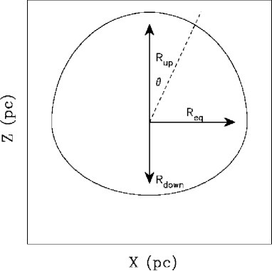
Figure 1: Sketch for an asymmetric SN.

2.2 A hyperbolic profile

The density is assumed to have the following dependence on $z$ in Cartesian coordinates,

$$\rho(z;z_{0},\rho_{0})=\begin{cases}\rho_{0}&\quad\text{if }z\leq z_{0}\\ \rho_{0}\frac{z_{0}}{z}&\quad\text{if }z>z_{0}\\ \end{cases}\quad,$$ (1)

where the parameter $z_{0}$ fixes the scale and $\rho_{0}$ is the density at $z=z_{0}$. In spherical coordinates the dependence on the polar angle is

$$\rho(r;\theta,z_{0},\rho_{0})=\begin{cases}\rho_{0}&\quad\text{if }r\cos(\theta)\leq z_{0}\\ \rho_{0}\frac{z_{0}}{r\cos(\theta)}&\quad\text{if }r\cos(\theta)>z_{0}\\ \end{cases}\quad.$$ (2)

Given a solid angle $\Delta\Omega$ the mass $M_{0}$ swept in the interval $[0,r_{0}]$ is

$$M_{0}=\frac{4}{3}\,\rho_{{0}}\pi\,{r_{{0}}}^{3}\Delta\Omega\quad.$$ (3)

The total mass swept, $M(r;r_{0},z_{0},\alpha,\theta,\rho_{0})$, in the interval $[0,r]$ is

$$M(r;r_{0},z_{0},\alpha,\theta,\rho_{0})=\bigl{(}\frac{4}{3}\,\rho_{{0}}\pi\,{r_{{0}}}^{3}+2\,{\frac{\rho_{{0}}{\it z_{0}}\,\pi\,\left({r}^{2}-{r_{{0}}}^{2}\right)}{\cos\left(\theta\right)}}\bigr{)}\Delta\Omega\quad.$$ (4)

The density $\rho_{0}$ can be obtained by introducing the number density expressed in particles $\mathrm{cm}^{-3}$, $n_{0}$, the mass of hydrogen, $m_{H}$, and a multiplicative factor $f$, which is chosen to be 1.4, see McCray (1987),

$$\rho_{0}=fm_{H}n_{0}\quad.$$ (5)

The astrophysical version of the total swept mass, expressed in solar mass units, $M_{\hbox{$\odot$}}$, is therefore

$$M(r_{pc};z_{0,pc},n_{0},\theta)\approx\frac{0.216\,n_{{0}}{\it z}_{{{\it 0,pc}}}{r_{{{\it pc}}}}^{2}}{cos(\theta)}\Delta\Omega\,M_{\hbox{$\odot$}}\quad,$$ (6)

where $z_{0,pc}$, $r_{0,pc}$ and $r_{0,pc}$ are $z_{0}$, $r_{0}$ and $r$ expressed in pc units.

2.3 A power law profile

The density is assumed to have the following dependence on $z$ in Cartesian coordinates:

$$\rho(z;z_{0},\rho_{0})=\begin{cases}\rho_{0}&\quad\text{if }z\leq z_{0}\\ \rho_{0}(\frac{z_{0}}{z})^{\alpha}&\quad\text{if }z>z_{0}\\ \end{cases}\quad,$$ (7)

where $z_{0}$ fixes the scale. In spherical coordinates, the dependence on the polar angle is

$$\rho(r,\theta,z_{0},\rho_{0})=\begin{cases}\rho_{0}&\quad\text{if }r\cos(\theta)\leq z_{0}\\ \rho_{0}(\frac{z_{0}}{r\cos(\theta)})^{\alpha}&\quad\text{if }r\cos(\theta)>z_{0}\\ \end{cases}$$ (8)

The mass $M_{0}$ swept in the interval $[0,r_{0}]$ in a given solid angle is

$$M_{0}=\frac{4}{3}\,\rho_{{0}}\pi\,{r_{{0}}}^{3}\Delta\Omega\quad.$$ (9)

The total mass swept, $M(r;r_{0},\alpha,\theta,\rho_{0})$, in the interval $[0,r]$ is

$$M(r;r_{0},\alpha,z_{0},\theta,\rho_{0})=\\ \bigg{(}\frac{4}{3}\,\rho_{{0}}\pi\,{r_{{0}}}^{3}-4\,{\frac{{r}^{3}\rho_{{0}}\pi}{\alpha-3}\left({\frac{{\it z_{0}}}{r\cos\left(\theta\right)}}\right)^{\alpha}}+4\,{\frac{\rho_{{0}}\pi\,{r_{{0}}}^{3}}{\alpha-3}\left({\frac{{\it z_{0}}}{r_{{0}}\cos\left(\theta\right)}}\right)^{\alpha}}\bigg{)}\Delta\Omega\quad.$$ (10)

The astrophysical swept mass is

$$M(r_{pc};z_{0,pc},\alpha,n_{0},\theta)\approx\frac{0.432\,n_{{0}}{{\it z}_{{{\it 0,pc}}}}^{\alpha}{r_{{{\it pc}}}}^{-\alpha+3}\left(\cos\left(\theta\right)\right)^{-\alpha}}{3-\alpha}\Delta\Omega\,M_{\hbox{$\odot$}}\quad.$$ (11)

2.4 An exponential profile

The density is assumed to have the following exponential dependence on $z$ in Cartesian coordinates:

$$\rho(z;b,\rho_{0})=\rho_{0}\exp{(-z/b)}\quad,$$ (12)

where $b$ represents the scale. In spherical coordinates, the density is

$$\rho(r;r_{0},b,\rho_{0})=\begin{cases}\rho_{0}&\quad\text{if }r\leq r_{0}\\ \rho_{0}\exp{-\frac{r\cos(\theta)}{b}}&\quad\text{if }r>r_{0}\\ \end{cases}$$ (13)

The total mass swept, $M(r;r_{0},b,\theta,\rho_{0})$, in the interval $[0,r]$ is

$$M(r;r_{0},b,\theta,\rho_{0})=\\ \frac{4}{3}\,\rho_{{0}}\pi\,{r_{{0}}}^{3}-4\,{\frac{b\left({r}^{2}\left(\cos\left(\theta\right)\right)^{2}+2\,rb\cos\left(\theta\right)+2\,{b}^{2}\right)\rho_{{0}}\pi}{\left(\cos\left(\theta\right)\right)^{3}}{{\rm e}^{-{\frac{r\cos\left(\theta\right)}{b}}}}}\\ +4\,{\frac{b\left({r_{{0}}}^{2}\left(\cos\left(\theta\right)\right)^{2}+2\,r_{{0}}b\cos\left(\theta\right)+2\,{b}^{2}\right)\rho_{{0}}\pi}{\left(\cos\left(\theta\right)\right)^{3}}{{\rm e}^{-{\frac{r_{{0}}\cos\left(\theta\right)}{b}}}}}\Delta\Omega\quad.$$ (14)

The astrophysical version expressed in solar masses is

$$M(r;r_{0,pc},b_{pc},\theta,n_{0})=\\ -\frac{1}{\left(\cos\left(\theta\right)\right)^{3}}\biggl{(}0.288\,n_{{0}}(-0.5\,{{\it r}_{{{\it 0,pc}}}}^{3}(\cos(\theta))^{3}+1.5\,{\it b_{pc}}\,{{\rm e}^{-1\,{\frac{r_{{{\it pc}}}\cos(\theta)}{{\it b_{pc}}}}}}{r_{{{\it pc}}}}^{2}(\cos(\theta))^{2}\\ +3.0\,{{\it b_{pc}}}^{2}{{\rm e}^{-1\,{\frac{r_{{{\it pc}}}\cos(\theta)}{{\it b_{pc}}}}}}r_{{{\it pc}}}\cos(\theta)+3.0\,{{\it b_{pc}}}^{3}{{\rm e}^{-1\,{\frac{r_{{{\it pc}}}\cos(\theta)}{{\it b_{pc}}}}}}\\ -1.5\,{\it b_{pc}}\,{{\rm e}^{-1\,{\frac{{\it r}_{{{\it 0,pc}}}\cos(\theta)}{{\it b_{pc}}}}}}{{\it r}_{{{\it 0,pc}}}}^{2}(\cos(\theta))^{2}\\ -3.0\,{{\it b_{pc}}}^{2}{{\rm e}^{-1\,{\frac{{\it r}_{{{\it 0,pc}}}\cos(\theta)}{{\it b_{pc}}}}}}{\it r}_{{{\it 0,pc}}}\cos(\theta)-3.0\,{{\it b_{pc}}}^{3}{{\rm e}^{-1\,{\frac{{\it r}_{{{\it 0,pc}}}\cos(\theta)}{{\it b_{pc}}}}}})\biggr{)}\Delta\Omega\,M_{\hbox{$\odot$}}\quad,$$ (15)

where $b_{pc}$ is the scale expressed in pc.

2.5 A Gaussian profile

The density is assumed to have the following Gaussian dependence on $z$ in Cartesian coordinates:

$$\rho(z;b,\rho_{0})=\rho_{0}{{\rm e}^{-\frac{1}{2}\,{\frac{{z}^{2}}{{b}^{2}}}}}\quad,$$ (16)

where $b$ represents the standard deviation. In spherical coordinates, the density is

$$\rho(r;r_{0},b,\rho_{0})=\begin{cases}\rho_{0}&\quad\text{if }r\leq r_{0}\\ \rho_{0}{{\rm e}^{-\frac{1}{2}\,{\frac{{z}^{2}}{{b}^{2}}}}}&\quad\text{if }r>r_{0}\\ \end{cases}\quad.$$ (17)

The total mass swept, $M(r;r_{0},b,\theta,\rho_{0})$, in the interval $[0,r]$ is

$$M(r;r_{0},b,\theta,\rho_{0})=\frac{4}{3}\,\rho 0\,\pi\,{{\it r_{0}}}^{3}+4\,\rho 0\,\pi\,\Bigl{(}-{\frac{r{b}^{2}}{(\cos(\theta))^{2}}{{\rm e}^{-\frac{1}{2}\,{\frac{{r}^{2}(\cos(\theta))^{2}}{{b}^{2}}}}}}\\ +\frac{1}{2}\,{\frac{{b}^{3}\sqrt{\pi}\sqrt{2}}{(\cos(\theta))^{3}}{\rm erf}(\frac{1}{2}\,{\frac{\sqrt{2}\cos(\theta)r}{b}})}\Bigr{)}-4\,\rho 0\,\pi\,\Bigl{(}-{\frac{{\it r_{0}}\,{b}^{2}}{(\cos(\theta))^{2}}{{\rm e}^{-\frac{1}{2}\,{\frac{{{\it r_{0}}}^{2}(\cos(\theta))^{2}}{{b}^{2}}}}}}\\ +\frac{1}{2}\,{\frac{{b}^{3}\sqrt{\pi}\sqrt{2}}{(\cos(\theta))^{3}}{\rm erf}(\frac{1}{2}\,{\frac{\sqrt{2}\cos(\theta){\it r_{0}}}{b}})}\Bigr{)}\Delta\Omega\quad,$$ (18)

where $\mathop{\mathrm{erf}}(x)$ is the error function, defined by

$$\mathop{\mathrm{erf}\/}\nolimits(x)=\frac{2}{\sqrt{\pi}}\int_{0}^{x}e^{-t^{2}}dt\quad.$$ (19)

The previous formula expressed is solar masses is

$$M(r;r_{0,pc},b_{pc},\theta,n_{0})=\\ \frac{1}{(\cos(\theta))^{3}}\Biggl{(}-1.024\,10^{-7}\,n_{{0}}\Bigl{(}-1.4\,10^{6}\,{{\it r}_{{{\it 0,pc}}}}^{3}(\cos(\theta))^{3}\\ +4.226\,10^{6}\,{{\rm e}^{-0.5\,{\frac{{r_{{{\it pc}}}}^{2}(\cos(\theta))^{2}}{{{\it b_{pc}}}^{2}}}}}r_{{{\it pc}}}{{\it b_{pc}}}^{2}\cos(\theta)\\ -5.297\,10^{6}\,{{\it b_{pc}}}^{3}{\rm erf}(0.707\,{\frac{\cos(\theta)r_{{{\it pcc}}}}{{\it b_{pc}}}})\\ -4.226\,10^{6}\,{{\rm e}^{-0.5\,{\frac{{{\it r}_{{{\it 0,pc}}}}^{2}(\cos(\theta))^{2}}{{{\it b_{pc}}}^{2}}}}}{\it r}_{{{\it 0,pc}}}{{\it b_{pc}}}^{2}\cos(\theta)\\ +5.297\,10^{6}\,{{\it b_{pc}}}^{3}{\rm erf}(0.707\,{\frac{\cos(\theta){\it r}_{{{\it pc}}}}{{\it b_{pc}}}})\Bigr{)}\Biggr{)}\Delta\Omega\,M_{\hbox{$\odot$}}\quad.$$ (20)

3 The classical thin layer approximation

The conservation of the classical momentum in spherical coordinates along the solid angle $\Delta\Omega$ in the framework of the thin layer approximation states that

$$M_{0}(r_{0})\,v_{0}=M(r)\,v\quad,$$ (21)

where $M_{0}(r_{0})$ and $M(r)$ are the swept masses at $r_{0}$ and $r$, and $v_{0}$ and $v$ are the velocities of the thin layer at $r_{0}$ and $r$. This conservation law can be expressed as a differential equation of the first order by inserting $v=\frac{dr}{dt}$:

$$M(r)\,\frac{dr}{dt}-M_{0}\,v_{0}=0\quad.$$ (22)

The above differential equation is independent of the azimuthal angle $\varphi$. The 3D surface which represents the advancing shock of the SN consists of the rotation about the $z$-axis of the curve in the $x-z$ plane defined by the analytical or numerical solution $r(t)$; this is the first symmetry. A second symmetry around the $z=0$ plane allows building the two lobes of the advancing surface. The orientation of the 3D surface is characterized by the Euler angles $(\Theta,\Phi,\Psi)$ and therefore by a total $3\times 3$ rotation matrix, $E$, see Goldstein et al. (2002).

The adopted astrophysical units are pc for length and yr for time; the initial velocity $v_{{0}}$ is expressed in pc yr^-1. The astronomical velocities are evaluated in  km s^-1 and therefore $v_{{0}}=1.02\times 10^{-6}v_{{1}}$ where $v_{{1}}$ is the initial velocity expressed in km s^-1.

3.1 The case of SN  1987A 

The complex structure of SN  1987A  can be classified as a torus only, a torus plus two lobes, and a torus plus 4 lobes, see Racusin et al. (2009). The region connected with the radius of the advancing torus is here identified with our equatorial region, in spherical coordinates, $\theta=\frac{\pi}{2}$. The radius of the torus only as a function of time can be found in Table 2 of Racusin et al. (2009) or Figure 3 of Chiad et al. (2012), see Figure 2 for a comparison of the two different techniques. The radius of the torus only as given by the counting pixels method (Chiad et al. (2012)) shows a more regular behavior and we calibrate our codes in the equatorial region in such a way that at time 23 years the radius is $\frac{0.39}{2}$ pc.

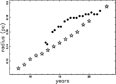
Figure 2: Observed radius of torus only as function of time: full points as in Racusin et al. 2009 and empty stars as in Chiad et al. 2012.

Another useful resource for calibration is a section of SN  1987A  reported as a sketch in Figure 5 of France et al. (2015). This section was digitized and rotated in the $x-z$ plane by $-40^{\,\circ}$, see Figure 3.

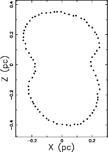
Figure 3: Section of SN  1987A  in the $x-z$ plane adapted by the author from Figure 5 in France et al. (2015).

The above approximate section allows introducing an observational percentage reliability, $\epsilon_{\mathrm{obs}}$, over the whole range of the polar angle $\theta$,

$$\epsilon_{\mathrm{obs}}=100(1-\frac{\sum_{j}|r_{\mathrm{obs}}-r_{\mathrm{num}}|_{j}}{\sum_{j}{r_{\mathrm{obs}}}_{,j}}),$$ (23)

where $r_{\mathrm{num}}$ is the theoretical radius, $r_{\mathrm{obs}}$ is the observed radius, and the index $j$ varies from 1 to the number of available observations, in our case 81. The above statistical method allows fixing the parameters of the theory in a scientific way rather than adopting an “ad hoc” hypothesis.

3.2 Motion with an hyperbolic profile

In the case of a hyperbolic density profile for the CSM as given by Eq. (1), the differential equation which models momentum conservation is

$$\left(\frac{4}{3}\,\rho_{{0}}\pi\,{r_{{0}}}^{3}+2\,{\frac{\rho_{{0}}{\it z_{0}}\,\pi\,\left(-{r_{{0}}}^{2}+\left(r\left(t\right)\right)^{2}\right)}{\cos\left(\theta\right)}}\right){\frac{\rm d}{{\rm d}t}}r\left(t\right)-\frac{4}{3}\,\rho_{{0}}\pi\,{r_{{0}}}^{3}v_{{0}}=0\quad,$$ (24)

where the initial conditions are $r=r_{0}$ and $v=v_{0}$ when $t=t_{0}$. The variables can be separated and the radius as a function of the time is

$$r(t;t_{0},z_{0},v_{0})=\frac{HN}{HD}\quad,$$

where

$$HN=r_{{0}}\sqrt[3]{3}(-2\,\cos(\theta)\sqrt[3]{3}r_{{0}}+(-9\,\cos(\theta)t_{{0}}v_{{0}}\sqrt{{\it z_{0}}}+9\,\cos(\theta)tv_{{0}}\sqrt{{\it z_{0}}}\\ +9\,\cos(\theta)r_{{0}}\sqrt{{\it z_{0}}}\\ -9\,{{\it z_{0}}}^{3/2}+\sqrt{3}\sqrt{\cos(\theta){\it AHN}})^{2/3}+3\,\sqrt[3]{3}{\it z_{0}})$$ (25)

with

$$AHN=27\,\cos(\theta){t}^{2}{v_{{0}}}^{2}{\it z_{0}}-54\,\cos(\theta)tt_{{0}}{v_{{0}}}^{2}{\it z_{0}}+27\,\cos(\theta){t_{{0}}}^{2}{v_{{0}}}^{2}{\it z_{0}}\\ +8\,(\cos(\theta))^{2}{r_{{0}}}^{3}+54\,\cos(\theta)r_{{0}}tv_{{0}}{\it z_{0}}\\ -54\,\cos(\theta)r_{{0}}t_{{0}}v_{{0}}{\it z_{0}}-9\,\cos(\theta){r_{{0}}}^{2}{\it z_{0}}-54\,tv_{{0}}{{\it z_{0}}}^{2}+54\,t_{{0}}v_{{0}}{{\it z_{0}}}^{2}$$ (26)

and

$$HD=3\,\sqrt{z_{{0}}}\sqrt[3]{{\it BHD}}$$ (27)

with

$$BHD=-9\,\cos\left(\theta\right)t_{{0}}v_{{0}}\sqrt{z_{{0}}}+9\,\cos\left(\theta\right)tv_{{0}}\sqrt{z_{{0}}}+9\,\cos\left(\theta\right)r_{{0}}\sqrt{z_{{0}}}\\ -9\,{z_{{0}}}^{3/2}+\sqrt{3}\sqrt{\cos\left(\theta\right){\it AHN}}\quad.$$ (28)

The velocity as a function of the radius $r$ is

$$v(t)=2\,{\frac{{r_{{0}}}^{3}v_{{0}}\cos\left(\theta\right)}{2\,{r_{{0}}}^{3}\cos\left(\theta\right)-3\,{r_{{0}}}^{2}z_{{0}}+3\,{r}^{2}z_{{0}}}}\quad.$$ (29)

Figure 4 displays a cut of SN  1987A  in the $x-z$ plane.

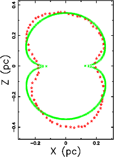
Figure 4: Section of SN  1987A  in the $x-z$ plane with a hyperbolic profile (green points) and observed profile (red stars). The parameters $r_{0}=0.06$ pc, $z_{0}=0.001$ pc, $t=21.86$ yr, $t_{0}=0.1$ yr and $v_{0}\,=25000$ km s^-1 give $\epsilon_{\mathrm{obs}}=92.13\%$.

A rotation around the $z$-axis of the previous section allows building a 3D surface, see Figure 5.

Figure 5: 3D surface of SN  1987A  with parameters as in Figure 4. The three Euler angles are $\Theta=40$, $\Phi=60$ and $\Psi=60$.

3.3 Motion with a power law profile

In the case of a power-law density profile for the CSM as given by Eq. (7), the differential equation which models the momentum conservation is

$$\frac{4}{3}\,\rho_{{0}}\pi\,{r_{{0}}}^{3}v_{{0}}-\bigl{(}\frac{4}{3}\,\rho_{{0}}\pi\,{r_{{0}}}^{3}-4\,{\frac{(r(t))^{3}\rho_{{0}}\pi}{\alpha-3}({\frac{z_{{0}}}{r(t)\cos(\theta)}})^{\alpha}}\\ +4\,{\frac{\rho_{{0}}\pi\,{r_{{0}}}^{3}}{\alpha-3}({\frac{z_{{0}}}{r_{{0}}\cos(\theta)}})^{\alpha}}\bigr{)}{\frac{\rm d}{{\rm d}t}}r(t)=0\quad.$$ (30)

The velocity is

$$v(r;r_{0},v_{0},\theta,\alpha)=\frac{-{r_{{0}}}^{3}v_{{0}}\left(\alpha-3\right)}{3\,\left({\frac{z_{{0}}}{r\cos\left(\theta\right)}}\right)^{\alpha}{r}^{3}-3\,\left({\frac{z_{{0}}}{r_{{0}}\cos\left(\theta\right)}}\right)^{\alpha}{r_{{0}}}^{3}-{r_{{0}}}^{3}\alpha+3\,{r_{{0}}}^{3}}\quad.$$ (31)

We now evaluate the following integral

$$I=\int_{r_{0}}^{r}\frac{1}{v(r;r_{0},v_{0},\theta,\alpha)}dr\quad,$$ (32)

which is

$$I_{p}(r)=3\,{\frac{{r}^{4}}{{r_{{0}}}^{3}v_{{0}}\left(\alpha-3\right)\left(\alpha-4\right)}{{\rm e}^{\alpha\,\ln\left({\frac{z_{{0}}}{r\cos\left(\theta\right)}}\right)}}}\\ +3\,{\frac{r}{v_{{0}}\left(\alpha-3\right)}\left({\frac{z_{{0}}}{r_{{0}}\cos\left(\theta\right)}}\right)^{\alpha}}+{\frac{\alpha\,r}{v_{{0}}\left(\alpha-3\right)}}-3\,{\frac{r}{v_{{0}}\left(\alpha-3\right)}}$$ (33)

The solution of the differential equation (30) can be found solving numerically the following nonlinear equation

$$I(r)-I(r_{0})=t-t_{0}\quad.$$ (34)

More precisely we used the FORTRAN SUBROUTINE ZBRENT from Press et al. (1992) and Figure 6 reports the numerical solution as a cut of SN  1987A  in the $x-z$ plane.

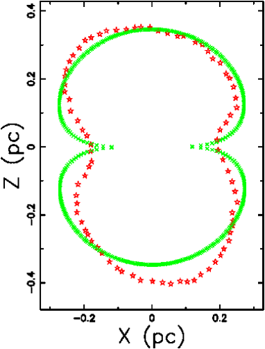
Figure 6: Section of SN  1987A  in the $x-z$ plane with a power law profile (green points) and observed profile (red stars). The parameters $r_{0}=0.05$ pc, $z_{0}=0.002$ pc, $t=21.86$ yr, $t_{0}=0.1$ yr, $\alpha=1.3$, $v_{0}\,=15000$  km s^-1 give $\epsilon_{\mathrm{obs}}=90.76\%$.

3.4 Motion with an exponential profile

In the case of an exponential density profile for the CSM as given by Eq. (12), the differential equation which models momentum conservation is

$$\Bigl{(}\frac{4}{3}\,\rho_{{0}}\pi\,{r_{{0}}}^{3}-4\,{\frac{b((r(t))^{2}(\cos(\theta))^{2}+2\,r(t)b\cos(\theta)+2\,{b}^{2})\rho_{{0}}\pi}{(\cos(\theta))^{3}}{{\rm e}^{-{\frac{r(t)\cos(\theta)}{b}}}}}\\ +4\,{\frac{b({r_{{0}}}^{2}(\cos(\theta))^{2}+2\,r_{{0}}b\cos(\theta)+2\,{b}^{2})\rho_{{0}}\pi}{(\cos(\theta))^{3}}{{\rm e}^{-{\frac{r_{{0}}\cos(\theta)}{b}}}}}\Bigr{)}{\frac{\rm d}{{\rm d}t}}r(t)\\ -\frac{4}{3}\,\rho_{{0}}\pi\,{r_{{0}}}^{3}v_{{0}}=0\quad.$$ (35)

An analytical solution does not exist and we present the following series solution of order 4 around $t_{0}$

$$r(t)=r_{{0}}+\left(t-{\it t_{0}}\right)v_{{0}}-3/2\,{\frac{{v_{{0}}}^{2}\left(t-{\it t_{0}}\right)^{2}}{r_{{0}}}{{\rm e}^{-{\frac{r_{{0}}\cos\left(\theta\right)}{b}}}}}\\ +\frac{1}{2}\,{\frac{{v_{{0}}}^{3}\left(t-{\it t_{0}}\right)^{3}}{{r_{{0}}}^{2}b}{{\rm e}^{-{\frac{r_{{0}}\cos\left(\theta\right)}{b}}}}\left(9\,{{\rm e}^{-{\frac{r_{{0}}\cos\left(\theta\right)}{b}}}}b+r_{{0}}\cos\left(\theta\right)-2\,b\right)}\\ +\mathcal{O}\left(t-t_{0}\right)^{4}\quad.$$ (36)

A second approximate solution can be found by deriving the velocity from (35):

$$v(r;r_{0},v_{0},\theta,b)=\frac{VN}{VD}$$ (37)

where

$$VN=-{r_{{0}}}^{3}v_{{0}}\left(\cos\left(\theta\right)\right)^{3}\quad,$$ (38)

and

$$VD=3\,{{\rm e}^{-{\frac{r\cos(\theta)}{b}}}}(\cos(\theta))^{2}b{r}^{2}-3\,{{\rm e}^{-{\frac{r_{{0}}\cos(\theta)}{b}}}}(\cos(\theta))^{2}{r_{{0}}}^{2}b-(\cos(\theta))^{3}{r_{{0}}}^{3}\\ +6\,{{\rm e}^{-{\frac{r\cos(\theta)}{b}}}}\cos(\theta){b}^{2}r-6\,{{\rm e}^{-{\frac{r_{{0}}\cos(\theta)}{b}}}}\cos(\theta)r_{{0}}{b}^{2}\\ +6\,{{\rm e}^{-{\frac{r\cos(\theta)}{b}}}}{b}^{3}-6\,{{\rm e}^{-{\frac{r_{{0}}\cos(\theta)}{b}}}}{b}^{3}\quad.$$ (39)

Given a function $f(r)$, the Padé approximant, after Padé (1892), is

$$f(r)=\frac{a_{0}+a_{1}r+\dots+a_{p}r^{p}}{b_{0}+b_{1}r+\dots+b_{q}r^{q}}\quad,$$ (40)

where the notation is the same of Olver et al. (2010). The coefficients $a_{i}$ and $b_{i}$ are found through Wynn’s cross rule, see Baker (1975); Baker and Graves-Morris (1996) and our choice is $p=2$ and $q=1$. The choice of $p$ and $q$ is a compromise between precision, high values for $p$ and $q$, and simplicity of the expressions to manage, low values for $p$ and $q$. The inverse of the velocity expressed by the the Padè approximant is

$$(\frac{1}{v(r)})_{2,1}=\frac{N21}{D21}\quad.$$ (41)

where

$$N21=(r-r_{{0}})(9\,{{\rm e}^{-{\frac{r_{{0}}\cos(\theta)}{b}}}}br-9\,{{\rm e}^{-{\frac{r_{{0}}\cos(\theta)}{b}}}}br_{{0}}\\ +2\,\cos(\theta)rr_{{0}}-2\,\cos(\theta){r_{{0}}}^{2}-4\,br+10\,r_{{0}}b)$$ (42)

and

$$D21=2\,v_{{0}}\left(\cos\left(\theta\right)rr_{{0}}-\cos\left(\theta\right){r_{{0}}}^{2}-2\,br+5\,r_{{0}}b\right)$$ (43)

The above result allows deducing a solution $r_{2,1}$ expressed through the Padè approximant

$$r(t)_{2,1}=\frac{B+\sqrt{A}}{9\,{{\rm e}^{-{\frac{r_{{0}}\cos\left(\theta\right)}{b}}}}b+2\,r_{{0}}\cos\left(\theta\right)-4\,b}$$ (44)

where

$$A=\left(\cos\left(\theta\right)\right)^{2}{r_{{0}}}^{2}{t}^{2}{v_{{0}}}^{2}-2\,\left(\cos\left(\theta\right)\right)^{2}{r_{{0}}}^{2}tt_{{0}}{v_{{0}}}^{2}+\left(\cos\left(\theta\right)\right)^{2}{r_{{0}}}^{2}{t_{{0}}}^{2}{v_{{0}}}^{2}\\ -4\,\cos\left(\theta\right)r_{{0}}b{t}^{2}{v_{{0}}}^{2}+8\,\cos\left(\theta\right)r_{{0}}btt_{{0}}{v_{{0}}}^{2}-4\,\cos\left(\theta\right)r_{{0}}b{t_{{0}}}^{2}{v_{{0}}}^{2}\\ +54\,{{\rm e}^{-{\frac{r_{{0}}\cos\left(\theta\right)}{b}}}}r_{{0}}{b}^{2}tv_{{0}}-54\,{{\rm e}^{-{\frac{r_{{0}}\cos\left(\theta\right)}{b}}}}r_{{0}}{b}^{2}t_{{0}}v_{{0}}+6\,\cos\left(\theta\right){r_{{0}}}^{2}btv_{{0}}\\ -6\,\cos\left(\theta\right){r_{{0}}}^{2}bt_{{0}}v_{{0}}+4\,{b}^{2}{t}^{2}{v_{{0}}}^{2}-8\,{b}^{2}tt_{{0}}{v_{{0}}}^{2}+4\,{b}^{2}{t_{{0}}}^{2}{v_{{0}}}^{2}-12\,r_{{0}}{b}^{2}tv_{{0}}\\ +12\,r_{{0}}{b}^{2}t_{{0}}v_{{0}}+9\,{b}^{2}{r_{{0}}}^{2}$$ (45)

and

$$B=r_{{0}}tv_{{0}}\cos\left(\theta\right)-r_{{0}}t_{{0}}v_{{0}}\cos\left(\theta\right)+9\,{{\rm e}^{-{\frac{r_{{0}}\cos\left(\theta\right)}{b}}}}br_{{0}}+2\,\cos\left(\theta\right){r_{{0}}}^{2}\\ -2\,btv_{{0}}+2\,bt_{{0}}v_{{0}}-7\,r_{{0}}b\quad.$$ (46)

Figure 7 compares the numerical solution, the approximate series solution, and the Padé approximant solution.

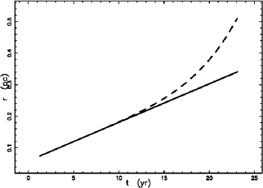
Figure 7: Numerical solution (full line) , power series solution (dashed line) and Padé approximant solution (dot-dash-dot-dash line), which is nearly equal to the numerical solution. The parameters are $r_{0}=0.06$ pc, $t=21.86$ yr, $t_{0}=0.1$ yr, $b=0.011$ pc, $\theta=0$, and $v_{0}\,=12000\ kms^{-1}$.

The above figure clearly shows the limited range of validity of the power series solution. The good agreement between the Padé approximant solution and numerical solution, in Figure 7 the two solutions can not be distinguished, has a percentage error

$$\epsilon=\frac{\big{|}r(t)-r(t)_{2,1}\big{|}}{r(t)}\times 100\quad,$$ (47)

where $r(t)$ is the numerical solution and $r(t)_{2,1}$ is the Padé approximant solution. Figure 8 shows the percentage error as a function of the polar angle $\theta$.

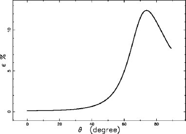
Figure 8: Percentage error of the Padé approximant solution compared to the numerical solution, as a function of the angle $\theta$ and other parameters as in Figure 7.

Figure 9 shows a cut of SN  1987A  in the $x-z$ plane evaluated with the numerical solution.

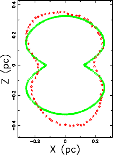
Figure 9: Section of SN  1987A  in the $x-z$ plane with an exponential profile (green points) and observed profile (red stars). The parameters are the same as Figure 7 and $\epsilon_{\mathrm{obs}}=90.66\%$.

3.5 Motion with a Gaussian profile

In the case of a Gaussian density profile for the CSM as given by Eq. (16), the differential equation which models momentum conservation is

$$\bigl{(}\frac{4}{3}\,\rho_{{0}}\pi\,{r_{{0}}}^{3}+4\,\rho_{{0}}\pi\,(-{\frac{r(t){b}^{2}}{(\cos(\theta))^{2}}{{\rm e}^{-\frac{1}{2}\,{\frac{(r(t))^{2}(\cos(\theta))^{2}}{{b}^{2}}}}}}\\ +\frac{1}{2}\,{\frac{{b}^{3}\sqrt{\pi}\sqrt{2}}{(\cos(\theta))^{3}}{\rm erf}(\frac{1}{2}\,{\frac{\sqrt{2}\cos(\theta)r(t)}{b}})})-4\,\rho_{{0}}\pi\,(-{\frac{r_{{0}}{b}^{2}}{(\cos(\theta))^{2}}{{\rm e}^{-\frac{1}{2}\,{\frac{{r_{{0}}}^{2}(\cos(\theta))^{2}}{{b}^{2}}}}}}\\ +\frac{1}{2}\,{\frac{{b}^{3}\sqrt{\pi}\sqrt{2}}{(\cos(\theta))^{3}}{\rm erf}(\frac{1}{2}\,{\frac{\sqrt{2}\cos(\theta)r_{{0}}}{b}})})\bigr{)}{\frac{\rm d}{{\rm d}t}}r(t)\\ -\frac{4}{3}\,\rho_{{0}}\pi\,{r_{{0}}}^{3}v_{{0}}=0\quad.$$ (48)

An analytical solution does not exist and Figure 10 shows a cut of SN  1987A  in the $x-z$ plane evaluated with a numerical solution.

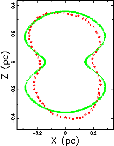
Figure 10: Section of SN  1987A  in the $x-z$ plane with a Gaussian profile (green points) and observed profile (red stars). The parameters $r_{0}=0.07$ pc, $t=21.86$ yr, $t_{0}=0.1$ yr, $b_{0}=0.018$ pc, $v_{0}=13000$ km s^-1 give $\epsilon_{\mathrm{obs}}=90.95\%$.

4 The relativistic thin layer approximation

The conservation of relativistic momentum in spherical coordinates along the solid angle $\Delta\Omega$ in the framework of the thin layer approximation gives

$${\frac{M\left(t;\theta\right)\beta}{\sqrt{1-{\beta}^{2}}}}\Delta\Omega={\frac{M_{{0}}\left(t_{{0}}\right)\beta 0}{\sqrt{1-{\beta 0}^{2}}}}\Delta\Omega\quad.$$ (49)

where $M_{0}(r_{0})$ and $M(r)$ are the swept masses at $r_{0}$ and $r$, $\beta=\frac{v}{c}$ , $\beta_{0}=\frac{v_{0}}{c}$, and $v_{0}$ and $v$ are the velocities of the thin layer at $r_{0}$ and $r$. We have chosen as units pc for distances and yr as time and therefore the speed of light is $c=0.306$ pc yr^-1.

4.1 Relativistic motion with a hyperbolic profile

In the case of a hyperbolic density profile for the CSM as given by Eq. (1), the differential equation which models the momentum conservation is

$$\left(\frac{4}{3}\,\rho_{{0}}\pi\,{r_{{0}}}^{3}+2\,{\frac{\rho_{{0}}{\it z_{0}}\,\pi\,\left(-{r_{{0}}}^{2}+\left(r\left(t\right)\right)^{2}\right)}{\cos\left(\theta\right)}}\right){\frac{\rm d}{{\rm d}t}}r\left(t\right)-\frac{4}{3}\,\rho_{{0}}\pi\,{r_{{0}}}^{3}v_{{0}}=0\quad,$$ (50)

where the initial conditions are $r=r_{0}$ and $v=v_{0}$ when $t=t_{0}$.

4.2 Relativistic motion with a hyperbolic profile

In the case of a hyperbolic density profile for the CSM as given by Eq. (1), the differential equation which models the relativistic momentum conservation is

$$\frac{2\,\rho_{{0}}\pi\,\left(2\,{r_{{0}}}^{3}\cos\left(\theta\right)+3\,{\it z0}\,\left(r\left(t\right)\right)^{2}-3\,{\it z0}\,{r_{{0}}}^{2}\right){\frac{\rm d}{{\rm d}t}}r\left(t\right)}{3\,\cos\left(\theta\right)c\sqrt{1-{\frac{\left({\frac{\rm d}{{\rm d}t}}r\left(t\right)\right)^{2}}{{c}^{2}}}}}-\frac{4\,\rho_{{0}}\pi\,{r_{{0}}}^{3}\beta_{{0}}}{3\,\sqrt{1-{\beta_{{0}}}^{2}}}=0\quad.$$ (51)

The velocity expressed in terms of $\beta$ can be derived from the above equation:

$$\beta=\frac{2\,{r_{{0}}}^{3}\cos\left(\theta\right)\beta_{{0}}}{D}\quad,$$ (52)

where

$$D=\Bigl{(}12\,{r_{{0}}}^{5}{\beta_{{0}}}^{2}{\it z0}\,\cos\left(\theta\right)-12\,{r_{{0}}}^{3}{\beta_{{0}}}^{2}{r}^{2}{\it z0}\,\cos\left(\theta\right)\\ +4\,{r_{{0}}}^{6}\left(\cos\left(\theta\right)\right)^{2}-9\,{r_{{0}}}^{4}{\beta_{{0}}}^{2}{{\it z0}}^{2}\\ +18\,{r_{{0}}}^{2}{\beta_{{0}}}^{2}{r}^{2}{{\it z0}}^{2}-9\,{\beta_{{0}}}^{2}{r}^{4}{{\it z0}}^{2}-12\,{r_{{0}}}^{5}{\it z0}\,\cos\left(\theta\right)\\ +12\,{r_{{0}}}^{3}{r}^{2}{\it z0}\,\cos\left(\theta\right)+9\,{r_{{0}}}^{4}{{\it z0}}^{2}-18\,{r_{{0}}}^{2}{r}^{2}{{\it z0}}^{2}+9\,{r}^{4}{{\it z0}}^{2}\Bigr{)}^{\frac{1}{2}}\quad.$$ (53)

An analytical solution of (51) does not exist, but we present the following series solution of order three around $t_{0}$:

$$r(t)=r_{{0}}+\beta_{{0}}c\left(t-{\it t0}\right)+\frac{3}{2}{\frac{{c}^{2}\left({\beta_{{0}}}^{2}-1\right)z_{{0}}{\beta_{{0}}}^{2}\left(t-{\it t0}\right)^{2}}{{r_{{0}}}^{2}\cos\left(\theta\right)}}+\mathcal{O}\left(t-t_{0}\right)^{3}\quad.$$ (54)

Figure 11 shows the numerical solution for SN  1987A  in the $x-z$ plane.

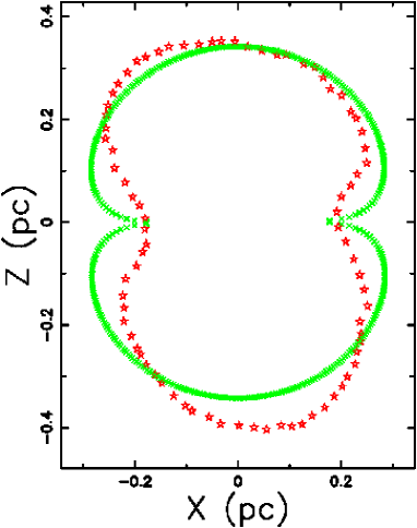
Figure 11: Section of SN  1987A  in the $x-z$ plane with a hyperbolic profile: relativistic case (green points) and observed profile (red stars). The parameters $r_{0}=0.1$ pc, $z_{0}=0.003$ pc, $t=21.86$ yr, $t_{0}=0.1$ yr, $v_{0}\,=78000$ km s^-1, and $\beta_{0}=0.26$ give $\epsilon_{\mathrm{obs}}=88.68\%$.

4.3 Relativistic motion with an exponential profile

In the case of an exponential density profile for the CSM as given by Eq. (12), the differential equation which models the relativistic momentum conservation is

$$\frac{N\,{\frac{\rm d}{{\rm d}t}}r(t)}{3\,\left(\cos\left(\theta\right)\right)^{3}c\sqrt{1-{\frac{\left({\frac{\rm d}{{\rm d}t}}r\left(t\right)\right)^{2}}{{c}^{2}}}}}-\frac{4\,\rho_{{0}}\pi\,{r_{{0}}}^{3}\beta_{{0}}}{3\,\sqrt{1-{\beta_{{0}}}^{2}}}=0\quad,$$ (55)

where

$$N=-4\,\rho_{{0}}\pi\,\Bigl{(}3\,(r(t))^{2}(\cos(\theta))^{2}{{\rm e}^{-{\frac{r(t)\cos(\theta)}{b}}}}b-(\cos(\theta))^{3}{r_{{0}}}^{3}\\ -3\,(\cos(\theta))^{2}{{\rm e}^{-{\frac{r_{{0}}\cos(\theta)}{b}}}}{r_{{0}}}^{2}b+6\,r(t)\cos(\theta){{\rm e}^{-{\frac{r(t)\cos(\theta)}{b}}}}{b}^{2}\\ -6\,\cos(\theta){{\rm e}^{-{\frac{r_{{0}}\cos(\theta)}{b}}}}r_{{0}}{b}^{2}-6\,{{\rm e}^{-{\frac{r_{{0}}\cos(\theta)}{b}}}}{b}^{3}+6\,{{\rm e}^{-{\frac{r(t)\cos(\theta)}{b}}}}{b}^{3}\Bigr{)}\quad.$$ (56)

An analytical solution of (56) does not exist, so we present the following series solution of order three around $t_{0}$:

$$r(t)=\\ r_{{0}}+c\beta_{{0}}\left(t-{\it t0}\right)+\frac{3}{2}\,{\frac{{\beta_{{0}}}^{2}{c}^{2}\left({\beta_{{0}}}^{2}-1\right)\left(t-{\it t0}\right)^{2}}{r_{{0}}}{{\rm e}^{-{\frac{r_{{0}}\cos\left(\theta\right)}{b}}}}}+\mathcal{O}\left(t-t_{0}\right)^{3}\quad.$$ (57)

Figure 12 shows the numerical solution for SN  1987A  in the $x-z$ plane.

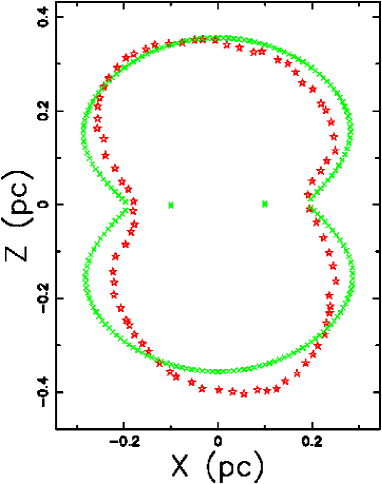
Figure 12: Section of SN  1987A  in the $x-z$ plane with an exponential profile: relativistic case (green points) and observed profile (red stars). The parameters $r_{0}$=0.1 pc, $b=0.02$ pc, $t=21.86$ yr, $t_{0}=0.1$ yr, $v_{0}\,=70000$ km s^-1, and $\beta_{0}=0.233$ give $\epsilon_{\mathrm{obs}}=90.23\%$.

5 Conclusions

Type of medium:

We have selected four density profiles, which decrease with the distance ($z$-axis) from the equatorial plane. The integral which evaluates the swept mass increases in complexity according to the following sequence of density profiles: hyperbolic, power law, exponential, and Gaussian.

Classical thin layer

The application of the thin layer approximation with different profiles produces differential equations of the first order. The solution of the first order differential equation can be analytical in the classical case characterized by a hyperbolic density profile, see (3.2), and numerical in all other cases. We also evaluated the approximation of the solution as a power law series, see (36), or using the Pade approximant, see (44): the differences between the two approximations are outlined in Figure 7.

Relativistic thin layer

The application of the thin layer approximation to the relativistic case produces first order differential equations which can be solved only numerically or as a power series, see (57) and (54).

The astrophysical case

The application of the theory here developed is connected with a clear definition of the advancing SN’s surface in 3D. We have concentrated the analysis on SN  1987A  with the cuts of the advancing surface in the $x-z$ plane when the $z$ axis is in front of the observer. Another choice of the point of view of the observer would complicate the situation, and a comparison between theory and observation then requires the introduction of the three Euler angles which characterize the observer, see the rotated advancing surface of SN  1987A  shown in Figure 5. Is interesting note that the rotation of the observed image with the polar axis aligned with the $z$-direction has been done for the Homunculus nebula, see Figure 4 in Smith (2006), but only an approximate section of the H-$\alpha$ imaging connected with SN  1987A  has been already reported, see Figure 5 in France et al. (2015). A more precise definition of the section of SN  1987A  will help the theoretical determination of the parameters maximizing the observational reliability, $\epsilon_{\mathrm{obs}}$, see 23. Is important note that the observational reliability gives already an acceptable result and $\epsilon_{\mathrm{obs}}$ lies within the interval [88%–92%] for the six models, four classical and two relativistic, here analyzed.

References

- Arthur and Falle (1993) Arthur, S. J. and Falle, S. A. E. G. (1993), “Supernova remnants in plane-stratified media—Predictions for H-alpha-emitting regions,” MNRAS , 261, 681–693.
- Baker (1975) Baker, G. (1975), Essentials of Padé approximants, New York: Academic Press.
- Baker and Graves-Morris (1996) Baker, G. A. and Graves-Morris, P. R. (1996), Padé Approximants, Cambridge: Cambridge University Press.
- Bisnovatyi-Kogan et al. (1989) Bisnovatyi-Kogan, G. S., Blinnikov, S. I., and Silich, S. A. (1989), “Supernova remnants and expanding supershells in inhomogeneous moving medium,” Astrophysics and Space Science , 154, 229–246.
- Blondin et al. (1996) Blondin, J. M., Lundqvist, P., and Chevalier, R. A. (1996), “Axisymmetric Circumstellar Interaction in Supernovae,” ApJ , 472, 257.
- Chevalier and Gardner (1974) Chevalier, R. A. and Gardner, J. (1974), “The Evolution of Supernova Remnants. 11. Models of an Explosion in a Plane-Stratified Medium,” ApJ , 192, 457–464.
- Chiad et al. (2012) Chiad, B. T., Karim, L. M., and Ali, L. T. (2012), “Study the Radial Expansion of SN 1987A Using Counting Pixels Method,” International Journal of Astronomy and Astrophysics, 2, 199–203.
- France et al. (2015) France, K., McCray, R., Fransson, C., Larsson, J., Frank, K. A., Burrows, D. N., Challis, P., Kirshner, R. P., Chevalier, R. A., Garnavich, P., Heng, K., Lawrence, S. S., Lundqvist, P., Smith, N., and Sonneborn, G. (2015), “Mapping High-velocity H and Ly Emission from Supernova 1987A,” ApJ , 801, L16.
- Gaensler (1998) Gaensler, B. M. (1998), “The Nature of Bilateral Supernova Remnants,” ApJ , 493, 781–792.
- Goldstein et al. (2002) Goldstein, H., Poole, C., and Safko, J. (2002), Classical Mechanics, San Francisco: Addison-Wesley.
- Igumenshchev et al. (1992) Igumenshchev, I. V., Tutukov, A. V., and Shustov, B. M. (1992), “Shapes of Supernova Remnants,” Soviet Astronomy, 36, 241.
- Lopez (2014) Lopez, L. A. (2014), “What Shapes Supernova Remnants?” in IAU Symposium, eds. Ray, A. and McCray, R. A., vol. 296 of IAU Symposium, pp. 239–244.
- Maciejewski and Cox (1999) Maciejewski, W. and Cox, D. P. (1999), “Supernova Remnant in a Stratified Medium: Explicit, Analytical Approximations for Adiabatic Expansion and Radiative Cooling,” ApJ , 511, 792–797.
- Marcaide et al. (2009) Marcaide, J. M., Martí-Vidal, I., Alberdi, A., and Pérez-Torres, M. A. (2009), “A decade of SN 1993J: Discovery of radio wavelength effects in the expansion rate,” A&A , 505, 927–945.
- Martí-Vidal et al. (2011) Martí-Vidal, I., Marcaide, J. M., Alberdi, A., Guirado, J. C., Pérez-Torres, M. A., and Ros, E. (2011), “Radio emission of SN1993J: The complete picture. I. Re-analysis of all the available VLBI data,” A&A , 526, A142+.
- McCray (1987) McCray, R. A. (1987), “Coronal interstellar gas and supernova remnants,” in Spectroscopy of Astrophysical Plasmas, ed. A. Dalgarno & D. Layzer, Cambridge: Cambridge University Press, pp. 255–278.
- Olver et al. (2010) Olver, F. W. J., Lozier, D. W., Boisvert, R. F., and Clark, C. W. (2010), NIST Handbook of Mathematical Functions, Cambridge: Cambridge University Press.
- Padé (1892) Padé, H. (1892), “Sur la représentation approchée d’une fonction par des fractions rationnelles,” Ann. Sci. Ecole Norm. Sup., 9, 193.
- Press et al. (1992) Press, W. H., Teukolsky, S. A., Vetterling, W. T., and Flannery, B. P. (1992), Numerical Recipes in FORTRAN. The Art of Scientific Computing, Cambridge: Cambridge University Press.
- Racusin et al. (2009) Racusin, J. L., Park, S., Zhekov, S., Burrows, D. N., Garmire, G. P., and McCray, R. (2009), “X-ray Evolution of SNR 1987A: The Radial Expansion,” ApJ , 703, 1752–1759.
- Silverman et al. (2015) Silverman, J. M., Vinkó, J., Marion, G. H., Wheeler, J. C., Barna, B., Szalai, T., Mulligan, B. W., and Filippenko, A. V. (2015), “High-velocity features of calcium and silicon in the spectra of Type Ia supernovae,” MNRAS , 451, 1973–2014.
- Smith (2006) Smith, N. (2006), “The Structure of the Homunculus. I. Shape and Latitude Dependence from H2 and Fe II Velocity Maps of eta Carinae,” ApJ , 644, 1151–1163.
- Zaninetti (2000) Zaninetti, L. (2000), “Large scale structures and synchrotron emission. I. Asymmetric supernova remnants,” A&A , 356, 1023–1030.
- Zaninetti (2012) — (2012), “On the spherical–axial transition in supernova remnants,” Astrophysics and Space Science, 337, 581–592.
- Zaninetti (2013) — (2013), “Three dimensional evolution of SN 1987A in a self-gravitating disk,” International Journal of Astronomy and Astrophysics, 3, 93–98.
- Zaninetti (2014) — (2014), “The Relativistic Three-Dimensional Evolution of SN 1987A,” International Journal of Astronomy and Astrophysics, 4, 359–364.
- Zhao et al. (2015) Zhao, X., Wang, X., Maeda, K., Sai, H., Zhang, T., Zhang, J., Huang, F., Rui, L., Zhou, Q., and Mo, J. (2015), “The Silicon and Calcium High-velocity Features in Type Ia Supernovae from Early to Maximum Phases,” ApJS , 220, 20.