TIFR/TH/16-37

Exact Growth of Entanglement and Dynamical Phase Transition in Global Fermionic Quench

Shruti Paranjape, and Nilakash Sorokhaibam

Department of Theoretical Physics

Tata Institute of Fundamental Research, Mumbai 400005, India.

Abstract

Critical quantum quench of free Dirac fermions in an infinite system is examined carefully. A much broader analysis, with more emphasis on free scalar fields, has been done in [1]. For specially prepared squeezed states of the massive theory, quenched states obtained are Calabrese-Cardy(CC) states and generalized Calabrese-Cardy(gCC) states with higher-spin charges. Exact time dependence of correlators are computed showing thermalization explicitly. We also calculate the exact monotonic growth of entanglement entropy in CC states. In case of gCC states, for a particular charge, we show that there is a dynamical phase transition from monotonic to non-monotonic entanglement entropy growth when the effective chemical potential is increased beyond a critical value.

1 Introduction and Summary

Thermalization in unitary quantum field theories has been a topic of great significance. Using AdS/CFT correspondence, it has also been linked to black hole formation [2, 3]. One of the current views of thermalization is that of the thermalization of a finite subsystem, in which the conjugate subsystem is considered the heat bath. In other words, it is the thermalization observed by an observer who has access to only a subsystem of the full system. It can also be considered as if the ‘fine-grained’ observables are spatially widely separated bilocal or higher point observables. Starting from a pure state, in the high energy (high effective temperature) limit, the final thermal entropy observed by such an observer is actually the entanglement entropy of the subsystem with its conjugate. Obviously, the pure state has to be a time-dependent state. Closely related to thermalization(equilibration in general), the study of time-dependent states after a quantum quench has also been of great interest[4, 5]. Quantum quench is the process in which the parameters of the Hamiltonian of a system in a certain state are changed with time. After the quantum quench, in the long time limit, if the subsystem of our interest looks like a thermal ensemble, in the sense that the expectation values of observables in the finite subsystem have the same expectation values as in a thermal ensemble, then we say that the system has thermalized. In this paper, we will be mainly considering quantum quench as the preparation of the time-dependent states of our interest.

We will also restrict ourself to critical quantum quenches, in which the final Hamiltonian is a critical Hamiltonian, i.e., the corresponding theory is a conformal field theory (CFT). More specifically, we will be considering free fermions in which starting from a certain state in the massive theory, the mass is set to zero gradually or suddenly. In more general theories, starting from the ground state of a gapped theory, it has been proposed [6, 7] that the state obtained after the critical quench is a Calabrese-Cardy(CC) state which has the form $e^{-\kappa_{2}H}|B\rangle$, where $\kappa_{2}$ is a scale given by the initial gap and the other scales of the quench process, $H$ is the Hamiltonian of the CFT and $|B\rangle$ is a conformally invariant boundary state. It has been shown that such a state thermalizes to a thermal ensemble with temperature $T=1/\beta=1/(4\kappa_{2})$. This result has also been generalised to the case in which the final theory has other conserved charges of local currents [8]. The corresponding ansatz for the state after quench from ground state is a generalized Calabrese-Cardy(gCC) states which have the form $e^{-\kappa_{2}H-\kappa_{4}W_{4}-\kappa_{6}W_{6}-...}|D\rangle$ where again the parameters $\kappa_{2},\kappa_{4},\kappa_{6},\cdots$ are given by the initial gap and other scales in the quench process, e.g. $\delta t=1/\rho$ the time taken to set the mass to zero, and $W_{4},W_{6},\cdots$ are the conserved charges of local currents. In this case also, it has been shown that the state thermalizes into a generalized Gibb’s Ensemble(GGE) with the density matrix $e^{-\beta H-\mu_{4}W_{4}-\mu_{6}W_{6}-...}$ where the corresponding temperature and chemical potentials are $T=1/\beta=1/(4\kappa_{2})$, $\mu_{4}=4\kappa_{4}$, $\mu_{6}=4\kappa_{6},\cdots$.

The gCC state ansatz has been shown to be true for mass quenches in free scalar and free fermion theories in a recent paper(MPS) [1]. Starting from the ground state of the massive theories, the quenched states obtained are of the gCC form with infinite number of charges $W_{2n}$ with $n\in\mathbb{N}$ ($W_{2}=H$). For the scalar theory, it was also found that naively taking the sudden limit when the mass profile is taken to be a step function, the final state is non-normalizable. For massless free scalar theory, $W_{2n}=\sum|k|^{2n-1}d^{\dagger}_{k}d_{k}$, where $d^{\dagger}_{k}$ and $d_{k}$ are the bosonic annihilation and creation operators. It was also shown that starting from specially prepared squeezed states of the massive scalar theory, CC state and gCC state with finite number of charges can also be created. By calculating correlators, thermalization of these states were explicitly shown.

In this paper, we find similar results for the fermionic mass quench. In the sudden limit, starting from the ground state, we observe that the final state has divergent energy density, $W_{4},W_{6},\cdots$. Again, as in the case of scalar fields in MPS, starting from specially prepared squeezed states using the sudden quench limit, we can prepare CC state and gCC state with a finite number of charges of our choice. For the CC state and the gCC state with finite number of charges, we calculate correlators and explicitly show thermalization to thermal ensemble and GGE respectively.

Among the other calculable quantities, entanglement entropy(EE) is the most interesting one. The EE growth has been calculated(mostly numerically) in many dynamical systems, see for e.g. [6, 11, 12, 13, 14, 15, 16]. It has also been extensively examined in holographic systems [17, 18, 19, 20, 21]. Recently, non-monotonic EE growth consisting of an initial dip around the quench time has also been observed in a holographic set-up in [22].

Since our final theory consists of only massless Dirac fermions, so using bosonization, we could calculate EE in some of our time-dependent states. We are interested in EE of a single interval only. For CC states, we find that EE grows monotonically. The asymptotic time limit is given by the well-known expression from CFT in a thermal ensemble, $S_{A}=\frac{c}{3}\log(\sinh(\frac{\pi r}{\beta}))$, where for Dirac fermions $c=1$ and the effective temperature $1/\beta=1/4\kappa$. In case of gCC states, we are not able to calculate EE with the charges of the usual fermionic bilinear $\mathcal{W}_{1+\infty}$ currents. But we are able to calculate the EE with the fermionic charge corresponding to the bosonic charges $W_{2n}=\sum|k|^{2n-1}d^{\dagger}_{k}d_{k}$. These are the charges of bosonic bilinear $\mathcal{W}_{2n}$ currents for $n>1$. For such gCC states with the $W_{4}$ charge, we found a dynamical phase transition in which EE grows non-monotonically when the effective chemical potential $\mu_{4}$ is greater than a critical value. Below this critical value, the EE growth is strictly monotonic.

In summary, the key results of the present work are:

1. For ground state quench, similar to the scalar quench, a naive sudden quench limit gives divergent conserved charges. Calculation of the correlators show equilibration explicitly. But the long distance and time and ultimately the stationary limit is significantly different from thermalization to a thermal ensemble. This is the same manifestation of the UV/IR mixing found in MPS.

2. Starting from appropriately prepared squeezed states of the massive theory, we can prepare CC and gCC states with specific $W_{2n}$ charges using quench. Calculation of correlators in CC state and gCC states explicitly show thermalization to thermal ensemble and GGE respectively. Here again, for gCC state, the long time and long distance limit of the correlators have significant dependence on the chemical potentials. This is again another avatar of the UV/IR mixing.

3. For CC state, we are able to calculate the growth of entanglement entropy of a single interval explicitly in analytic form. The EE growth is strictly monotonically increasing for CC state. The stationary limit is, as expected, the entanglement entropy of a single interval in thermal ensemble.

4. We also calculate the EE growth of a single interval in gCC state with $W_{4}$ charge of the $\mathcal{W}_{2n}$ representation of fermion corresponding to the $\mathcal{W}_{2n}$ bilinear bosonic representation. We find dynamical phase transition in which the EE growth is monotonically increasing upto a critical value of $\kappa_{4}$. Beyond the critical value, the EE growth is non-monotonic.

The outline of the paper is as follows:

In section 2, we solve the Dirac equation with time-dependent mass and from explicit solutions for a specific mass profile, we calculate the Bogoliubov coefficients for the transformation between the massive and massless modes. In section 3, we find the final state after the quench starting from the ground state and a few squeezed states of our interest. In sections 4 and 5, we calculate energy density and some correlators in the different quenched states that we obtained. The EE growth of a single subsystem in CC state is explicitly calculated in section 6. In section 7, we show the dynamical phase transition in the EE growth of a subsystem in a particular gCC state. Section 8 contains some discussions. The appendix contains details that we have omitted in the main sections.

2 Free Dirac fermions with time-dependent mass

The action for Dirac fermions with time-dependent mass is

$$S=-\int dx^{2}\left[i\bar{\Psi}\gamma^{\mu}\partial_{\mu}\Psi-m(t)\bar{\Psi}\Psi\right]\$$ (1)

The equation of motion (EOM) is

$$\left[i\gamma^{0}\partial_{t}-i\gamma^{1}\partial_{x}-m(t)\right]\Psi(x,t)=0\$$ (2)

and we are interested in the solvable mass profile[23, 24]

$$m(t)=m[1-\tanh(\rho t)]/2\$$ (3)

$m$ is the initial mass and $\rho$ is the only scale of the quench process. $\rho\to\infty$ is the sudden limit in which the mass is set to zero suddenly - much faster than any other length scale in the theory. It is easier to solve (2) in the Dirac basis in which $\gamma_{0}$ is diagonal. Since the system is translation invariant in the spatial $x$-direction, the solution ansatz is

$$\Psi(x,t)=\left[\gamma^{0}\partial_{t}-\gamma^{1}\partial_{x}-im(t)\right]e^{\pm ikx}\Phi(t)\$$ (4)

Substitution in the EOM gives,

$$\left[\partial^{2}_{t}+k^{2}+m(t)^{2}-i\gamma^{0}\dot{m}(t)\right]e^{\pm ikx}\Phi(t)=0\$$

where $\dot{m}(t)=\partial_{t}m(t)$.

$\Phi(t)$ is solved in the eigenbasis of $\gamma^{0}$. For the two eigenvalues of $\gamma^{0}$ (1 and -1), the two solutions $\phi_{+}(t)$ and $\phi_{-}(t)$ are given by,

$$\left[\partial^{2}_{t}+k^{2}+m(t)^{2}-i\dot{m}(t)\right]\phi_{+}(t)=0$$

$$\left[\partial^{2}_{t}+k^{2}+m(t)^{2}+i\dot{m}(t)\right]\phi_{-}(t)=0\$$ (5)

where $\Phi(t)=\begin{bmatrix}\phi_{+}(t)&\phi_{-}(t)\end{bmatrix}^{\text{T}}$. The eigenstates of $\gamma^{0}$ are $u_{0}=\begin{bmatrix}1\\ 0\end{bmatrix}$ and $v_{0}=\begin{bmatrix}0\\ 1\end{bmatrix}$, they are the spinors in the rest frame.

For the mass profile (3), there are two important bases of solutions in which we are interested in. The first one is the ‘in’ basis in which the two independent solutions of the second order linear differential equations become different single frequency modes in the $t\to-\infty$ limit. In other words, one solution becomes the negative energy mode and the other solution becomes the positive energy mode. Similarly, there is also an ‘out’ basis of solutions in which one solution becomes the negative energy mode and the other becomes the positive energy mode in the $t\to\infty$ limit. Accordingly, we will also have different ‘in’ and ‘out’ creation and annihilation operators. Consider the solutions of (5) in the two bases to be

$$\phi_{\pm}(t,k)=\phi_{in,\pm p}(t,k)+\phi_{in,\pm m}(t,k)$$ (6)

$$\phi_{\pm}(t,k)=\phi_{out,\pm p}(t,k)+\phi_{out,\pm m}(t,k)\$$ (7)

where the limits are

$$\lim_{t\to-\infty}\phi_{in,\pm p}(t,k)=e^{-i\omega_{in}t},\quad\lim_{t\to-\infty}\phi_{in,\pm m}(t,k)=e^{i\omega_{in}t}$$

$$\lim_{t\to\infty}\phi_{out,\pm p}(t,k)=e^{-i\omega_{out}t},\quad\lim_{t\to\infty}\phi_{out,\pm m}(t,k)=e^{i\omega_{out}t}\$$

where ‘p’ means positive energy and ‘m’ means negative energy. The above solutions are the same but written in two different bases for simplicity in the appropriate time limits, they are related by Bogoliubov transformations.
But from (5), we see that the equations of $\phi_{+}$ and $\phi_{-}$ are the complex conjugates of each other, so

$$\phi_{in,+p}(t,k)=\phi^{*}_{in,-m}(t,k),\quad\phi_{in,+m}(t,k)=\phi^{*}_{in,-p}(t,k)$$ (8)

$$\phi_{out,+p}(t,k)=\phi^{*}_{out,-m}(t,k),\quad\phi_{out,+m}(t,k)=\phi^{*}_{out,-p}(t,k)\$$ (9)

The Bogoliubov transformations are

$$\phi_{in,+p}(t,k) = \alpha^{\prime}_{+}(k)\phi_{out,+p}(t,k)+\beta^{\prime}_{+}(k)\phi_{out,+m}(t,k)$$ (10)

$$= \alpha^{\prime}_{+}(k)\phi_{out,+p}(t,k)+\beta^{\prime}_{+}(k)\phi^{*}_{out,-p}(t,k)$$

$$\phi_{in,-p}(t,k) = \alpha^{\prime}_{-}(k)\phi_{out,-p}(t,k)+\beta^{\prime}_{-}(k)\phi_{out,-m}(t,k)$$ (11)

$$= \alpha^{\prime}_{-}(k)\phi_{out,-p}(t,k)+\beta^{\prime}_{-}(k)\phi^{*}_{out,+p}(t,k)\$$

where $\alpha^{\prime}_{\pm}(k)$ an $\beta^{\prime}_{\pm}(k)$ are actually functions of $|k|$, since the equations of motion have only $k^{2}$ terms.

Now, suppressing the basis labels ‘in’ and ‘out’ since they apply to both bases, we write the $u_{0}$ part of $\Psi(x,t)$ as (upto normalization)

$$\tilde{U}(x,t;k)=\left[\gamma^{0}\partial_{t}+\gamma^{1}\partial_{x}-im(t)\right]e^{ikx}\phi_{+p}(t)\begin{bmatrix}1\\ 0\end{bmatrix}\$$ (12)

And the $v_{0}$ part of $\Psi(x,t)$ as

$$\tilde{V}(x,t;k) = \left[\gamma^{0}\partial_{t}+\gamma^{1}\partial_{x}-im(t)\right]e^{-ikx}\phi_{-m}(t)\begin{bmatrix}0\\ 1\end{bmatrix}$$ (13)

$$= \left[\gamma^{0}\partial_{t}+\gamma^{1}\partial_{x}-im(t)\right]e^{-ikx}\phi^{*}_{+p}(t)\begin{bmatrix}0\\ 1\end{bmatrix}\$$

We can define the spinors as (upto normalization)

$$\tilde{u}(t,k) = \frac{1}{e^{ikx}\phi_{+p}(t)}\tilde{U}(x,t;k)$$

$$\tilde{v}(t,k) = \frac{1}{e^{-ikx}\phi_{-m}(t)}\tilde{V}(x,t;k)\$$

With proper normalization, the final Dirac fermion mode expansion is

$$\Psi(x,t) = \int\frac{dk}{2\pi}\frac{1}{\sqrt{2\omega}}\left[a_{k}U(x,t;k)+b^{\dagger}_{k}V(x,t;k)\right]$$ (14)

$$= \int\frac{dk}{2\pi}\frac{1}{\sqrt{2\omega}}\left[a_{k}u(t;k)e^{ikx}\phi_{+p}(t)+b^{\dagger}_{k}v(t;k)e^{-ikx}\phi_{-m}(t)\right]\$$

2.1 Bogoliubov transformation of oscillators

The initial mass is taken to be $\lim_{t\to-\infty}m(t)=m$. It is convenient to take the final mass $\lim_{t\to\infty}m(t)$ to be some $m_{out}$, because of the spinor convention (in P&S), although we are interested in $m_{out}=0$.

With time-dependent mass, as mentioned above, the spinors are functionals of $m(t)$, but their normalizations are constants or else they will not solve the Dirac equations. So, we have to differentiate between ‘in’ spinors and ‘out’ spinors. Taking this into account, the mode expansion of $\Psi(x,t)$ starting from ‘in’ basis to ‘out’ basis is

$$\Psi(x,t) = \int\frac{dk}{2\pi}\frac{1}{\sqrt{2\omega_{in}}}\left[a_{in,k}u_{in}(k,m)\phi_{in,+p}(t,k)e^{ikx}+b^{\dagger}_{in,k}v_{in}(k,m)\phi^{*}_{in,+p}(t,k)e^{-ikx}\right]$$

$$= \int\frac{dk}{2\pi}\frac{1}{\sqrt{2\omega_{in}}}\Huge{[}\{\alpha^{\prime}_{+}(k)a_{in,k}u_{in}(k,m)\phi_{out,+p}(t,k)+b^{\dagger}_{in,-k}v_{in}(-k,m)\beta^{\prime*}_{+}(k)\phi_{out,-p}(t,k)\}e^{ikx}$$

$$\quad+\{\alpha^{\prime*}_{+}(k)b^{\dagger}_{in,k}v_{in}(k,m)\phi^{*}_{out,+p}(t,k)+a_{in,-k}u_{in}(-k,m)\beta^{\prime}_{+}(k)\phi^{*}_{out,-p}(t,k)\}e^{-ikx}\huge{]}$$

where we have used the facts that the $k$ integral is from $-\infty$ to $\infty$ and $\alpha^{\prime}_{\pm}$, $\beta^{\prime}_{\pm}$ and $\phi_{\pm p}$ are functions of $|k|$. In $t\to\infty$ limit, $m(t)\to m_{out}$, so,

$$\lim_{t\to\infty}\Psi(x,t) = \int\frac{dk}{2\pi}\frac{1}{\sqrt{2\omega_{out}}}\sqrt{\frac{\omega_{out}}{\omega_{in}}}\huge{[}\{\alpha^{\prime}_{+}(k)a_{in,k}u_{in}(k,m_{out})+b^{\dagger}_{in,-k}v_{in}(-k,m_{out})\beta^{\prime*}_{+}(k)\}e^{-ik\cdot x}$$

$$\quad+\{\alpha^{\prime*}_{+}(k)b^{\dagger}_{in,k}v_{in}(k,m_{out})+a_{in,-k}u_{in}(-k,m_{out})\beta^{\prime}_{+}(k)\}e^{ik\cdot x}\huge{]}\$$

Comparing with the mode expansion in the ‘out’ solution basis in the same limit $t\to\infty$,

$$\lim_{t\to\infty}\Psi(x,t) = \int\frac{dk}{2\pi}\frac{1}{\sqrt{2\omega_{out}}}\left[a_{out,k}u_{out}(k,m_{out})\phi_{out,+p}(t,k)e^{ikx}+b^{\dagger}_{out,k}v_{out}(k,m_{out})\phi^{*}_{out,+p}(t,k)e^{-ikx}\right]\$$

we get the Bogoliubov transformations of the creation and annihilation operators.

$$a_{out,k} = \alpha_{+}(k)a_{in,k}+b^{\dagger}_{in,-k}\,\chi(k,m_{out})\beta^{*}_{+}(k)$$ (16)

$$b^{\dagger}_{out,k} = \alpha^{*}_{+}(k)b^{\dagger}_{in,k}+a_{in,-k}\,\tilde{\chi}(k,m_{out})\beta_{+}(k)\$$ (17)

where $\alpha_{+}(k)=\sqrt{\frac{\omega_{out}(\omega_{out}+m_{out})}{\omega_{in}(\omega_{in}+m_{in})}}\,\alpha^{\prime}_{+}$ and $\beta_{+}(k)=\sqrt{\frac{\omega_{out}(\omega_{out}+m_{out})}{\omega_{in}(\omega_{in}+m_{in})}}\,\beta^{\prime}_{+}(k)$. Using (LABEL:norspinor)

$$\chi(k,m_{out}) = \frac{1}{2m_{out}}\sqrt{\frac{\omega_{in}+m_{in}}{\omega_{out}+m_{out}}}\,\bar{u}_{out}(k,m_{out},\omega_{out})v_{in}(-k,m_{out},-\omega_{out})$$ (18)

$$= \text{sgn}(k)\qquad\qquad\text{when}\quad m_{out}\to 0\$$

where we have to be careful that $v_{in}(k,m_{out})$ is a functional of the accompanying mode, which is $\sim e^{-i\omega_{out}t}$ in the above case. Similarly, with $m_{out}\to 0$,

$$\tilde{\chi}(k) = -\frac{1}{2m_{out}}\sqrt{\frac{\omega_{in}+m_{in}}{\omega_{out}+m_{out}}}\,\bar{v}(k,m_{out},\omega_{out})u(-k,m_{out},\omega_{out})=\text{sgn}(k)\$$ (19)

taking into account the normalization of $\bar{v}_{out}v_{out}=-2m_{out}$. Inverting (16) and (17), we get

$$a_{in,k} = \alpha^{*}_{+}(k)a_{out,k}-\text{sgn}(k)\beta^{*}_{+}(k)b^{\dagger}_{out,-k}$$ (20)

$$b^{\dagger}_{in,-k} = \alpha_{+}(k)b^{\dagger}_{out,-k}+\text{sgn}(k)\beta_{+}(k)a_{out,k}\$$ (21)

From here on, we will suppress the subscript ‘out’ on creation and annihilation operators, so $a_{out,k}=a_{k}$, similarly for $b_{out,k}$ and their Hermitian conjugates. Also, since $\chi(k)$ and $\tilde{\chi}(k)$ are simple sign functions, with a slight abuse of the nomenclature, we will call $\alpha_{+}(k)$ and $\beta_{+}(k)$ as the Bogoluibov coefficients. Moreover, $\chi(k)^{2}$ and $\tilde{\chi}(k)^{2}$ are identically equal to 1. So, the fermionic anti-commutation relations of the ‘in’ and ‘out’ operators constraint the Bogoluibov coefficients as

$$|\alpha_{+}(k)|^{2}+|\beta_{+}(k)|^{2}=1\$$ (22)

2.2 Explicit solutions

In the ‘in’ basis, for our choice of mass profile, the solutions are

$$\phi_{in,+p} = e^{-it\left(\omega+m\right)}\left(e^{-2\rho t}+1\right)^{-\frac{im}{2\rho}}\ _{2}F_{1}\left(\frac{i\left(|k|-m-\omega\right)}{2\rho},-\frac{i\left(|k|+m+\omega\right)}{2\rho};1-\frac{i\omega}{\rho};-e^{2t\rho}\right)$$

$$\phi_{in,-m} = e^{it\left(\omega-m\right)}\left(e^{-2\rho t}+1\right)^{-\frac{im}{2\rho}}\ _{2}F_{1}\left(\frac{i\left(-|k|-m+\omega\right)}{2\rho},\frac{i\left(|k|-m+\omega\right)}{2\rho};\frac{i\omega}{\rho}+1;-e^{2t\rho}\right)\$$

where $\omega=\sqrt{k^{2}+m^{2}}$. While in the ‘out’ basis, the solutions are

$$\phi_{out,+p} = e^{-i|k|t}\left(e^{-2\rho t}+1\right)^{-\frac{im}{2\rho}}\ _{2}F_{1}\left(\frac{i|k|-im+i\omega}{2\rho},\frac{i|k|-im-i\omega}{2\rho};1+\frac{i|k|}{\rho};-e^{-2\rho t}\right)$$

$$\phi_{out,-m} = e^{i|k|t}\left(e^{-2\rho t}+1\right)^{-\frac{im}{2\rho}}\ _{2}F_{1}\left(\frac{-i|k|-im+i\omega}{2\rho},\frac{-i|k|-im-i\omega}{2\rho};1-\frac{i|k|}{\rho};-e^{-2\rho t}\right)\$$

Using the properties of confluent hypergeometric functions ${}_{2}F_{1}$ given in [25], the Bogoliubov coefficients of the frequency modes as defined in (10) are

$$\alpha^{\prime}_{+} = \frac{\Gamma\left(-\frac{i|k|}{\rho}\right)\Gamma\left(1-\frac{i\omega}{\rho}\right)}{\Gamma\left(-\frac{i\left(|k|+m+\omega\right)}{2\rho}\right)\Gamma\left(1+\frac{-i|k|+im-i\omega}{2\rho}\right)}$$ (23)

$$\beta^{\prime}_{+} = \frac{\Gamma\left(\frac{i|k|}{\rho}\right)\Gamma\left(1-\frac{i\omega}{\rho}\right)}{\Gamma\left(1-\frac{i\left(-|k|-m+\omega\right)}{2\rho}\right)\Gamma\left(-\frac{i\left(-|k|+m+\omega\right)}{2\rho}\right)}$$ (24)

In the sudden limit($\rho\to\infty$). the Bogoliubov coefficients of the frequency modes are

$$\alpha^{\prime}_{+}(k) = \frac{|k|+m_{in}+\sqrt{k^{2}+m^{2}}}{2|k|}$$ (25)

$$\beta^{\prime}_{+}(k) = \frac{|k|-m_{in}-\sqrt{k^{2}+m^{2}}}{2|k|}\$$ (26)

As mentioned above, for a quench starting from the ground state of the massive theory, the naive sudden limit gives a non-normalizable state in the massless theory [1]. The problem arises only for a quench starting from the ground state. In case the quench is starting from squeezed states of our interest, the naive sudden limit given above works well. As defined in (16) and (17), the Bogoluibov coefficients of the oscillator modes differ from $\alpha^{\prime}_{+}(k)$ and $\beta^{\prime}_{+}(k)$ by an overall factor.

$$\alpha_{+} = \sqrt{1-\frac{m}{\sqrt{k^{2}+m^{2}}}}\frac{\Gamma\left(-\frac{i|k|}{\rho}\right)\Gamma\left(1-\frac{i\omega}{\rho}\right)}{\Gamma\left(-\frac{i\left(|k|+m+\omega\right)}{2\rho}\right)\Gamma\left(1+\frac{-i|k|+im-i\omega}{2\rho}\right)}$$ (27)

$$\beta_{+} = \sqrt{1-\frac{m}{\sqrt{k^{2}+m^{2}}}}\frac{\Gamma\left(\frac{i|k|}{\rho}\right)\Gamma\left(1-\frac{i\omega}{\rho}\right)}{\Gamma\left(1-\frac{i\left(-|k|-m+\omega\right)}{2\rho}\right)\Gamma\left(-\frac{i\left(-|k|+m+\omega\right)}{2\rho}\right)}$$ (28)

In the sudden limit, they are

$$\alpha_{+}(k) = \sqrt{1-\frac{m}{\sqrt{k^{2}+m^{2}}}}\,\frac{|k|+m+\sqrt{k^{2}+m^{2}}}{2|k|}$$ (29)

$$\beta_{+}(k) = \sqrt{1-\frac{m}{\sqrt{k^{2}+m^{2}}}}\,\frac{|k|-m-\sqrt{k^{2}+m^{2}}}{2|k|}\$$ (30)

For completeness, the expressions of $\alpha^{\prime}_{-}$ and $\beta^{\prime}_{-}$ in (11) for our particular quench protocol are

$$\alpha^{\prime}_{-} = \frac{\Gamma\left(-\frac{i\left|k\right|}{\rho}\right)\Gamma\left(1-\frac{i\omega}{\rho}\right)}{\Gamma\left(-\frac{i\left(\left|k\right|-m+\omega\right)}{2\rho}\right)\Gamma\left(1-\frac{i\left(\left|k\right|+m+\omega\right)}{2\rho}\right)}$$ (31)

$$\beta^{\prime}_{-} = \frac{\Gamma\left(\frac{i\left|k\right|}{\rho}\right)\Gamma\left(1-\frac{i\omega}{\rho}\right)}{\Gamma\left(\frac{i\left(\left|k\right|+m-\omega\right)}{2\rho}\right)\Gamma\left(1-\frac{i\left(-\left|k\right|+m+\omega\right)}{2\rho}\right)}$$ (32)

3 Quenched states

3.1 From ground state

Starting from the ground state of the massive theory $|\Psi\rangle=|0,in\rangle$, using Eq (20), the state in terms of ‘out’ operators is given by

$$a_{in,k}|\Psi\rangle=0\quad \Rightarrow\left[\alpha^{*}_{+}(k)a_{k}-\text{sgn}(k)\beta^{*}_{+}(k)b^{\dagger}_{-k}\right]|\Psi\rangle=0$$

$$\Rightarrow|\Psi\rangle=e^{\sum_{k}\text{sgn(k)}\gamma(k)a^{\dagger}_{k}b^{\dagger}_{-k}}|0\rangle$$ (33)

where $$\quad\gamma(k)=\frac{\alpha^{*}_{+}(k)}{\beta^{*}_{+}(k)}\$$ (34)

where we have taken $|0\rangle$ to be the ground state of ‘out’ oscillators. Using the Baker-Campbell-Hausdorff(BCH) formula derived in appendix (E), the above state can be written in gCC form. For the particular mass profile (3), $\alpha_{+}(k)$ and $\beta_{+}(k)$ are given in (27) and (28). The gCC form which was first obtained in MPS is

$$|\Psi\rangle=e^{-\kappa_{2}H-\kappa_{4}W_{4}-\kappa_{6}W_{6}-...}|D\rangle\$$ (35)

where

$$\kappa_{2}=\frac{1}{2m}+\frac{\pi^{2}m}{12\rho^{2}}+\frac{1}{m}\mathcal{O}\left(\frac{m}{\rho}\right)^{3},\quad\kappa_{4}=-\frac{1}{12m^{3}}+\frac{\pi^{2}}{24m\rho^{2}}+\frac{1}{m^{3}}\mathcal{O}\left(\frac{m}{\rho}\right)^{3},$$

$$\kappa_{6}=\frac{3}{80m^{5}}-\frac{\pi^{2}}{96m^{3}\rho^{2}}+\frac{1}{m^{5}}\mathcal{O}\left(\frac{m}{\rho}\right)^{3},...\$$ (36)

and $|D\rangle$ is the Dirichelet state and the explicit expression is in Appendix C. It should be noted that since the mass does not go to zero at any finite time, the above state should is only valid in sufficiently long time limit and the correction due to the non-vanishing mass is $\mathcal{O}(e^{-\rho t})$.

3.2 From squeezed states: CC state and gCC states

We could start with specially prepared squeezed states so that after the quench, the states become CC states or gCC states. Here, we will consider only the simple case of sudden quench ($\rho\to\infty$). For our aim of creating a CC state or a gCC state, finite ‘$\rho$’ quenches are an unnecessary complication.

We start with a squeezed state of ‘in’ modes

$$|S\rangle=\exp\left(\sum_{k=-\infty}^{\infty}f(k)a^{\dagger}_{in,k}b^{\dagger}_{in,-k}\right)|0,in\rangle\$$ (37)

where unlike $\gamma(k)$, $f(k)$ need not be an even function of $k$, but $|f(k)|^{2}$ is an even function of $k$.

It is easier to work with $|S\rangle$ as an operator relation. $|S\rangle$ can also be defined as

$$\tilde{a}_{k}|S\rangle=\tilde{b}_{k}|S\rangle=0\ \text{and} \left\{\tilde{a}_{k},\tilde{a}^{\dagger}_{k^{\prime}}\right\}=\left\{\tilde{b}_{-k},\tilde{b}^{\dagger}_{-k^{\prime}}\right\}=\delta(k-k^{\prime})\$$ (38)

where the new operators in terms of the out modes using (20) and (21) are

$$\tilde{a}_{k} =\frac{1}{\sqrt{(1+|f(k)|^{2})}}a_{in,k}-\frac{f(k)}{\sqrt{(1+|f(k)|^{2})}}b^{\dagger}_{in,-k}$$

$$=A^{*}(k)a_{out,k}-\text{sgn}(k)B^{*}(k)b_{out,-k}$$

$$\tilde{b}_{-k} =\frac{1}{\sqrt{(1+|f(k)|^{2})}}b_{in,-k}+\frac{f(k)}{\sqrt{(1+|f(k)|^{2})}}a^{\dagger}_{in,k}$$

$$=A^{*}(k)b_{out,-k}+\text{sgn}(k)B^{*}(k)a^{\dagger}_{out,k}\$$ (39)

where $A(k)$ and $B(k)$ are the Bogoliubov coefficients for the transformation from ‘tilde’ operators to ‘out’ operators and are given by

$$A(k)=\frac{\alpha_{+}(k)-\text{sgn}(k)\beta_{+}^{*}(k)f^{*}(k)}{\sqrt{(1+|f(k)|^{2})}},\quad B(k)=\frac{\beta_{+}(k)+\text{sgn}(k)\alpha_{+}^{*}(k)f^{*}(k)}{\sqrt{(1+|f(k)|^{2})}}$$ (40)

$$|A(k)|^{2}+|B(k)|^{2}=1\$$ (41)

Now using the BCH formula (133) from appendix (E),

$$|S\rangle=\exp\left\{-\sum_{k}\tilde{\kappa}(k)\left(a^{\dagger}_{out,k}a_{out,k}+b^{\dagger}_{out,k}b_{out,k}\right)\right\}|D\rangle$$ (42)

$$\text{where}\quad\tilde{\gamma}(k)=\frac{B^{*}(k)}{A^{*}(k)},\quad\text{and}\quad\tilde{\kappa}(k)=-\frac{1}{2}\log(\tilde{\gamma}(k))\$$

For a CC state, i.e., so that $|S\rangle$ in eqn (42) is $e^{-\kappa_{2}H}|D\rangle$, $f(k)$ should be tuned as

$$f(k)=\frac{\left(\sqrt{k^{2}+m^{2}}+m\right)\cosh(\kappa_{2}k)-k\sinh(\kappa_{2}k)}{\left(\sqrt{k^{2}+m^{2}}+m\right)\sinh(\kappa_{2}k)+k\cosh(\kappa_{2}k)}\$$ (43)

Starting with

$$f(k)=\frac{k-k\,e^{2\left|k\right|\left(\kappa_{2}+\kappa_{4}k^{2}\right)}+\text{sgn}(k)\left(\sqrt{k^{2}+m^{2}}+m\right)\left(e^{2\left|k\right|\left(\kappa_{2}+\kappa_{4}k^{2}\right)}+1\right)}{\left|k\right|\left(e^{2\left|k\right|\left(\kappa_{2}+\kappa_{4}k^{2}\right)}+1\right)+\left(\sqrt{k^{2}+m^{2}}+m\right)\left(e^{2\left|k\right|\left(\kappa_{2}+\kappa_{4}k^{2}\right)}-1\right)}\$$ (44)

we get a gCC state of the form $e^{-\kappa_{2}H-\kappa_{4}W_{4}}|D\rangle$, where as mentioned earlier, $W_{4}$ is the conserved charge of the $\mathcal{W}_{4}$ current of free Dirac fermions. Note that $f(k)$ are odd functions of $k$. For future reference, we can invert Eq (39) and we write down the ‘in’ and ‘out’ operators in terms of the ‘tilde’ operators.

$$a_{in,k}=\frac{1}{\sqrt{(1+|f(k)|^{2})}}\tilde{a}_{k}+\frac{f(k)}{\sqrt{(1+|f(k)|^{2})}}\tilde{b}^{\dagger}_{-k}$$ (45)

$$b^{\dagger}_{in,-k}=\frac{1}{\sqrt{(1+|f(k)|^{2})}}\tilde{b}^{\dagger}_{-k}-\frac{f^{*}(k)}{\sqrt{(1+|f(k)|^{2})}}\tilde{a}_{k}$$ (46)

$$a_{out,k}=A(k)\tilde{a}_{k}+\text{sgn}(k)B^{*}(k)\tilde{b}^{\dagger}_{-k}$$ (47)

$$b^{\dagger}_{out,-k}=A^{*}(k)\tilde{b}^{\dagger}_{-k}-\text{sgn}(k)B(k)\,\tilde{a}_{k}\$$ (48)

4 Energy density

In the post-quench theory, the occupation number is given by

$$\hat{N}_{k}=a_{k}^{\dagger}a_{k}+b_{k}^{\dagger}b_{k}\$$ (49)

using the Bogoliubov transformations (47) and (48) and definition of $|\tilde{0}\rangle$ in (38), the expectation value of the occupation number is given by

$$N_{k} = \lim_{t\to\infty}\langle\tilde{0}|a_{k}^{\dagger}a_{k}+b_{k}^{\dagger}b_{k}|\tilde{0}\rangle$$ (50)

$$= B^{*}(k)B(k)\langle\tilde{0}|\tilde{b}_{-k}^{\dagger}\tilde{b}_{-k}|\tilde{0}\rangle+B^{*}(-k)B(-k)\langle\tilde{0}|\tilde{a}_{-k}^{\dagger}\tilde{a}_{-k}|\tilde{0}\rangle+...$$

$$= B^{*}(k)B(k)+B^{*}(-k)B(-k)\$$

The expression of $B(k)$ is given in (40). For ground state, we have to use $f(k)=0$ in the expression of $B(k)$. So, energy density of the post-quench state is given by

$$E=\int_{-\infty}^{\infty}\frac{dk}{2\pi}|k|\left[B^{*}(k)B(k)+B^{*}(-k)B(-k)\right]\$$ (51)

Ground state quench

For ground state quench, the occupation number is given by

$$N_{k} = \lim_{t\to\infty}\langle 0,in|\hat{N}_{k}|0,in\rangle=|\beta_{+}(k)|^{2}+|\beta_{+}(-k)|^{2}\$$

Since $\alpha_{+}(k)$ and $\beta_{+}(k)$ are even functions of $k$. Using (22), (34) and (134), we have

$$|\beta_{+}(k)|^{2}=\frac{|\gamma(k)|^{2}}{1+|\gamma(k)|^{2}},\qquad|\gamma(k)|^{2}=e^{-4\kappa(k)}\$$ (52)

Hence, the occupation number in the ground state in the asymptotically long time limit is given by

$$N_{k}=\frac{2}{e^{4\kappa(k)}+1}\$$ (53)

This is the occupation number in a GGE defined as

$$\text{Tr}\,e^{-\sum_{k}4\kappa(k)\hat{N}_{k}}=\text{Tr}e^{-4\kappa_{2}H-4\kappa_{4}W_{4}-\kappa_{6}W_{6}-\cdots}\$$ (54)

where the $\kappa$’s are given in (36). Using the expressions of $\beta_{+}(k)$ from (28), the explicit expression of the occupation number is

$$N_{k} = \text{csch}\left(\frac{\pi k}{\rho}\right)\left(\cosh\left(\frac{\pi m}{\rho}\right)-\cosh\left(\frac{\pi\left(k-\sqrt{k^{2}+m^{2}}\right)}{\rho}\right)\right)\text{csch}\left(\frac{\pi\sqrt{k^{2}+m^{2}}}{\rho}\right)$$

$$\xrightarrow{\rho\to\infty} 1-\frac{k}{\sqrt{k^{2}+m^{2}}}\$$

It is interesting that in $m\to\infty$ limit, $N_{k}\to 1$, not 2. This is because $\lim_{\rho\to\infty}|\alpha_{+}(k)|^{2}=1/2$ and we have the constraint $|\alpha_{+}(k)|^{2}+|\beta_{+}(k)|^{2}=1$.
For arbitrary $\rho$, the energy density cannot be calculated in closed form. In the sudden limit $\rho\to\infty$, the energy density diverges as $\log(\Lambda)$ where $\Lambda$ is the UV cutoff. Hence, all other $W$ charges also diverge in the sudden limit. Hence, naively taking $\rho\to\infty$ produce a non-renormalizable state. So, the sudden limit has to be taken as in MPS where $m/\Lambda\to 0$ while $m/\rho\to\epsilon^{+}$. Simply put, the quench rate parameter $\rho$ should be much small than the UV cut-off.

Squeezed state quench: CC and gCC states

For CC state given by (43), the expectation value of occupation number is given by

$$N_{k}=\frac{2}{1+e^{4\kappa_{2}\left|k\right|}}\$$ (55)

This is the occupation number of fermions in a thermal ensemble of temperature $1/\beta=1/4\kappa_{2}$. The enengy density is

$$E=\int_{-\infty}^{\infty}\frac{dk}{2\pi}N_{k}=\frac{\pi}{96\kappa_{2}^{2}}\$$ (56)

Similarly, for gCC state given by (44), the expectation value of occupation number is given by

$$N_{k}=\langle gCC|\hat{N}_{k}|gCC\rangle=\frac{2}{1+e^{4\kappa_{2}\left|k\right|+4\kappa_{4}\left|k\right|^{3}}}\$$ (57)

This is same as the occupation number of fermions in a generalised Gibbs ensemble of temperature $1/\beta=4\kappa_{2}$ and chemical potential $\mu_{4}=4\kappa_{4}$ of $W_{4}$ charge. The enengy density cannot be calculated in closed form.

5 Correlation functions

Since our theory is a free theory, all the observables can be explicitly calculated. In the following subsections we calculate $\langle\psi^{\dagger}(r,t)\psi(0,t)\rangle$ correlation functions for the three different states obtained above. The quench process cannot differentiate between holomorphic dof(‘left-movers’) and anti-holomorphic dof(‘right-movers’), so $\langle\bar{\psi}^{\dagger}(0,t)\bar{\psi}(r,t)\rangle$ is equal to $\langle\psi^{\dagger}(r,t)\psi(0,t)\rangle$ and they are time independent quantities. We also calculated $\langle\bar{\psi}^{\dagger}(r,t)\psi(0,t)\rangle$ which has non-trivial time-dependence. Also as expected, $-\langle\psi^{\dagger}(0,t)\bar{\psi}(r,t)\rangle$ is the complex conjugate of $\langle\bar{\psi}^{\dagger}(r,t)\psi(0,t)\rangle$. Since, we are calculating equal-time correllation functions, so for example for $\langle\psi^{\dagger}(r,t)\psi(0,t)\rangle$, we would rather be calculating $\frac{1}{2}\langle\psi^{\dagger}(r,t)\psi(0,t)-\psi(0,t)\psi^{\dagger}(r,t)\rangle$.
Using the Bogoluibov transformations (47) and (48) in the chiral mode expansions (116) and (117) we get

$$\psi(w) =\int_{0}^{\infty}\frac{dk}{2\pi}\Big{[}A(k)\tilde{a}_{k}e^{-ikw}+\text{sgn}(k)B^{*}(k)\tilde{b}^{\dagger}_{-k}e^{-ikw}+A^{*}(-k)\tilde{b}^{\dagger}_{k}e^{ikw}+\text{sgn}(k)B(-k)\tilde{a}_{-k}e^{ikw}\Big{]}$$ (58)

$$\bar{\psi}(\bar{w}) =\int^{\infty}_{0}\frac{dk}{2\pi}\Big{[}A(-k)\tilde{a}_{-k}e^{-ik\bar{w}}-\text{sgn}(k)B^{*}(-k)\tilde{b}^{\dagger}_{k}e^{-ik\bar{w}}-A^{*}(k)\tilde{b}^{\dagger}_{-k}e^{ik\bar{w}}+\text{sgn}(k)B(k)\tilde{a}_{k}e^{ik\bar{w}}\Big{]}\$$ (59)

where $w=t-x$ and $\bar{w}=t+x$. For the ground state quench, $f(k)=0,\,\tilde{a}_{k}=a_{in,k},\,\tilde{b}=b_{in,k}$ and $|\tilde{0}\rangle=|0,in\rangle$.
For a general $f(k)$ corresponding to some $|\tilde{0}\rangle$, the correlation functions are

$$\langle\tilde{0}|\psi^{\dagger}(0,t)\psi(r,t)|\tilde{0}\rangle = \frac{1}{2}\int_{0}^{\infty}\frac{dk}{2\pi}\left[(2|B(k)|^{2}-1)e^{ikr}-(2|B(-k)|^{2}-1)e^{-ikr}\right]$$ (60)

$$\langle\tilde{0}|\bar{\psi}^{\dagger}(0,t)\psi(r,t)|\tilde{0}\rangle = -\int_{0}^{\infty}\frac{dk}{2\pi}\left[\text{sgn}(k)A^{*}(-k)B(-k)e^{ik(2t-r)}+\text{sgn}(k)A(k)B^{*}(k)e^{-ik(2t-r)}\right]$$

where we have used (41) to write $A(k)$ in terms of $B(k)$ in the first equation.

Ground state quench:

Taking careful limit, for ground state quench, we have

$$\langle 0,in|\psi^{\dagger}(0,t)\psi(r,t)|0,in\rangle =-\frac{1}{2}\int_{-\infty}^{\infty}\frac{dk}{2\pi}\frac{\left|k\right|}{\sqrt{k^{2}+m^{2}}}$$ (62)

$$=\frac{1}{4}m\left[\boldsymbol{L}_{-1}(mr)-I_{1}(mr)\right]$$

$$\xrightarrow{m\to\infty}\frac{1}{2\pi mr^{2}}+\frac{3}{2\pi m^{3}r^{4}}+O\left(\frac{1}{m^{4}}\right)$$

$$\langle\tilde{0}|\bar{\psi}^{\dagger}(0,t)\psi(r,t)|\tilde{0}\rangle =\int_{0}^{\infty}\frac{dk}{2\pi}\,\frac{i\,\text{sgn}(k)\,m\sin(k(2t-r))}{\sqrt{k^{2}+m^{2}}}$$ (63)

$$=-\frac{im}{4}\,\left[\text{sgn}(r-2t)I_{0}(m(r-2t))-\boldsymbol{L}_{0}(m(r-2t))\right]$$

$$\xrightarrow[t>r/2]{m\to\infty}\frac{i}{2\pi(2t-r)}+\frac{i}{2\pi m^{2}(2t-r)^{3}}+O\left(\frac{1}{m^{4}}\right)\$$

where $I_{\nu}(x)$ is Modified Bessel Function of the First Kind and $\boldsymbol{L}_{\nu}(x)$ is Modified Struve Function.

Quenched squeezed state - CC state:

For CC state, all the calculations are done in $|S_{CC}\rangle$ defined as the state (37) with the expression of $f(k)$ given in (43).

$$\langle CC|\psi^{\dagger}(0,t)\psi(r,t)|CC\rangle = -i\int_{0}^{\infty}\frac{dk}{2\pi}\,\tanh(2\kappa_{2}|k|)\sin(kr)$$ (64)

$$= -i\int_{0}^{\infty}\frac{dk}{2\pi}\,\sin(kr)\left[\frac{1}{e^{4\kappa_{2}|k|}+1}-\frac{1}{2}\right]$$ (65)

$$= -\frac{i\,\text{csch}\left(\frac{\pi r}{4\kappa_{2}}\right)}{8\kappa_{2}}$$ (66)

$$\langle CC|\bar{\psi}^{\dagger}(0,t)\psi(r,t)|CC\rangle = -i\int_{0}^{\infty}\frac{dk}{2\pi}\,\text{sech}(2k\kappa_{2})\cos(k(2t-r))$$ (67)

$$= -\frac{i\,\text{sech}\left(\frac{\pi(2t-r)}{4\kappa_{2}}\right)}{8\kappa_{2}}\$$ (68)

These are exactly what have been calculated using BCFT techniques [26]. It is evident from (65) that $\psi^{\dagger}\psi$ expectation value is already the thermal expectation value at temperature $T=1/\beta=1/(4\kappa_{2})$, i.e., it is already thermalized.

Quenched squeezed state - gCC state with $W_{4}$:

Similarly, for gCC state, all the calculations are done in $|S_{fCC}\rangle$ defined as the state (37) with the expression of $f(k)$ given in (44).

$$\langle\psi^{\dagger}(0,t)\psi(r,t)\rangle_{gCC} = -i\int_{0}^{\infty}\frac{dk}{2\pi}\,\tanh\left(2\kappa_{2}|k|+2\kappa_{4}|k|^{3}\right)\,\sin(kr)$$ (69)

$$= -i\int_{0}^{\infty}\frac{dk}{2\pi}\,\sin(kr)\left[\frac{1}{e^{4\kappa_{2}|k|+4\kappa_{4}|k|^{3}}+1}-\frac{1}{2}\right]$$ (70)

$$\langle\bar{\psi}^{\dagger}(r,t)\psi(0,t)\rangle_{gCC} = -i\int_{0}^{\infty}\frac{dk}{2\pi}\,\text{sech}(2\kappa_{2}k+2\kappa_{4}k^{3})\cos(k(2t-r))\$$ (71)

Again, it is evident from (70) that $\psi^{\dagger}\psi$ expectation value is already thermalized into the expectation value in a GGE with $T=1/\beta=1/4\kappa_{2}$ and $\mu=4\kappa_{4}$. A possible way of evaluating these integrals (which yield no closed form answer) is via the residue theorem. The integrands in both cases, have poles at the solutions of $2\kappa_{2}k+2\kappa_{4}k^{3}=\frac{2n+1}{2}i\pi$, where $n\in\mathbb{Z}$. These poles and their residues have been treated in detail in [1]. The sum of residues is still an infinite sum which cannot be performed. In the perturbative regime ($\kappa_{4}/\kappa_{2}^{3}<<1$), we see that our correlators match the general form presented in [8] with $h=1/2$ as expected.

As expected form MPS, here in the fermionic theory also we see the UV/IR mixing. For the ground state quench, all the charges affect the long distance and long time limit of the correlators. This is explicit seen in the case of gCC state with $W_{4}$ charge only. The long time and large distance limit or the correlators are very much dependent upon $k_{4}$, although a naive Wilsonian RG argument would show that $k_{4}$ is an irrelevant coupling.

6 Exact Growth of Entanglement in CC state

We will consider only a finite single interval or subsystem A, with its endpoints at $(w_{1},\bar{w}_{1})$ and $(w_{2},\bar{w}_{2})$ in light-cone coordinates, or $(0,t)$ and $(r,t)$ in space and time coordinates. Using the replica trick ([27], [28]), the $n\textsuperscript{th}$ Rényi entropy $S_{n}(A)$ of the interval is given by the logarithm of the expectation value of twist and antitwist operators inserted at the end-points.

$$S_{n}(A)=\frac{1}{1-n}\log\langle\Psi(t)|\mathcal{T}_{n}(w_{1},\bar{w}_{1})\tilde{\mathcal{T}}_{n}(w_{2},\bar{w}_{2})|\Psi(t)\rangle\$$ (72)

The entanglement entropy(EE) $S_{A}$ is given by $\lim_{n\to 1}S_{n}(A)$. We can diagonalize the twist operators and write them as products of twist fields. Hence,

$$\mathcal{T}_{n}(w,\bar{w})=\prod_{k=-(n-1)/2}^{k=(n-1)/2}\mathcal{T}_{k,n}(w,\bar{w}),\quad\tilde{\mathcal{T}}_{n}(w,\bar{w})=\prod_{k=-(n-1)/2}^{k=(n-1)/2}\tilde{\mathcal{T}}_{k,n}(w,\bar{w})\$$ (73)

In CC state, in Heisenberg picture, the quantity of our interest is

$$Z_{k}=\langle D_{f}|e^{-\kappa_{2}H_{f}}\mathcal{T}_{k,n}(0,t)\tilde{\mathcal{T}}_{k,n}(r,t)e^{-\kappa_{2}H_{f}}|D_{f}\rangle\$$ (74)

The subscript ‘f’ means we are working in the fermionic theory and the subscript ‘b’ would mean we are working in the bosonic theory. To find the exact expression of the entanglement entropy of a spatial region in our free fermionic CFT, we will use the method using bosonization described in [29]. Moreover, as shown in Appendix(D), Dirichlet state $|D_{f}\rangle$ in fermionic theory corresponds to a Dirichlet state in the bosonic theory $|D_{b}\rangle$ and $H_{f}$ corresponds to $H_{b}$. So, we get

$$Z_{k} = \langle D_{b}|e^{-\kappa_{2}H_{b}}e^{i\sqrt{4\pi}\frac{k}{n}\left(\phi(0,t)-\phi(r,t)\right)}e^{-\kappa_{2}H_{b}}|D_{b}\rangle\$$ (75)

This is a free scalar theory in a strip geometry with Dirichlet boundary conditions and operator insertions at $(0,t)$ and $(r,t)$. It can be calculated explicitly

$$\log\left[Z_{k}\right] = -4\pi\,\frac{2k^{2}}{n^{2}}\left(\langle\phi(0,t)\phi(0,t)\rangle-\langle\phi(0,t)\phi(r,t)\rangle\right)\$$ (76)

The $n\textsuperscript{th}$ Rényi entropy of interval A is given by

$$S_{n}(A) = -4\pi\frac{1}{1-n}\sum_{k=-(n-1)/2}^{k=(n-1)/2}\frac{2k^{2}}{n^{2}}\left(\langle\phi(0,t)\phi(0,t)\rangle-\langle\phi(0,t)\phi(r,t)\rangle\right)$$ (77)

$$= 4\pi\,\frac{n+1}{6n}\,\left(\langle\phi(0,t)\phi(0,t)\rangle-\langle\phi(0,t)\phi(r,t)\rangle\right)\$$

Taking $n\to 1$ limit, we get the entanglement entropy,

$$S_{A}=4\pi\,\frac{1}{3}\,\left(\langle\phi(0,t)\phi(0,t)\rangle-\langle\phi(0,t)\phi(r,t)\rangle\right)\$$ (78)

Remark on winding number: While the free boson considered in MPS [1] is the uncompactified free boson, the boson in (75) is a compactified free boson. So, Hamiltonian of the compactifed boson has zero mode terms but the winding number is not important for our analysis. In the large system size limit($L\to\infty$), the zero modes vanished. Even if we are taking the limiting case of a finite size system, the zero momentum modes do not play any role in our calculation. Using the mode expansion of the boson $\phi(w,\bar{w})=\varphi(w)+\bar{\varphi}(\bar{w})$ in [30],

$$\varphi(w) = Q+\frac{P}{2L}\,w+\sum_{n>0}\frac{1}{\sqrt{4\pi n}}\left(d_{n}e^{-inw}+d^{\dagger}_{n}e^{inw}\right)$$ (79)

$$\bar{\varphi}(\bar{w}) = \bar{Q}+\frac{\bar{P}}{2L}\,\bar{w}+\sum_{n>0}\frac{1}{\sqrt{4\pi n}}\left(d_{-n}e^{-in\bar{w}}+d^{\dagger}_{-n}e^{in\bar{w}}\right)\$$ (80)

First, $Q$ and $\bar{Q}$ are cancelled identically in (75). Moreover, by bosonization formulae [30, 31],

$$P =\sqrt{4\pi}N_{f} \bar{P} =\sqrt{4\pi}\bar{N}_{f}$$ (81)

$$N_{f} =J_{0}=-\sum_{k=0}^{\infty}\left[a^{\dagger}_{k}a_{k}-b^{\dagger}_{k}b_{k}\right] \bar{N}_{f} =\bar{J}_{0}=-\sum_{k=0}^{\infty}\left[a^{\dagger}_{-k}a_{-k}-b^{\dagger}_{-k}b_{-k}\right]\$$ (82)

But for our particular CC state, from (131), $N_{f}|CC_{f}\rangle=0$ and $\bar{N}_{f}|CC_{f}\rangle=0$. Now, $P$ and $\bar{P}$ commute with all the other bosonic creation and annihilation operators of non-zero momentum, hence they don’t play any role in the calculation of (75). If we still keep the system size finite, the winding number would be important to interpret the stationary limit as a thermal ensemble. But we must take the $L\to\infty$ limit, if we want to examine the stationary limit. In other words, $L$ is the largest length scale in our theory and time $t<<L$.

The bosonic propagator in CC state has been calculated in [1]. It is given by

$$\langle CC|\phi(0,t)\phi(r,t)|CC\rangle=-\frac{1}{8\pi}\log\left(\frac{2\sinh^{2}\left(\frac{\pi r}{4\kappa_{2}}\right)}{\cosh\left(\frac{\pi r}{2\kappa_{2}}\right)+\cosh\left(\frac{\pi t}{\kappa_{2}}\right)}\right)\$$ (83)

$r\to 0$ gives the UV divergence of scalar field theory in 2D spacetime. The $n\textsuperscript{th}$ Rényi entropy and entanglement entropy of interval A in CC state is given by

$$S_{n}(A) = \frac{n+1}{12n}\,\left[\log\left(\frac{\sinh^{2}\left(\frac{\pi r}{4\kappa_{2}}\right)\left(1+\cosh\left(\frac{\pi t}{\kappa_{2}}\right)\right)}{\cosh\left(\frac{\pi r}{2\kappa_{2}}\right)+\cosh\left(\frac{\pi t}{\kappa_{2}}\right)}\right)-\lim_{\epsilon\to 0+}2\log(\epsilon)-\log\left(\frac{\pi^{2}}{16\kappa_{2}^{2}}\right)\right]$$

$$S_{A} = \frac{1}{3}\,\left[\frac{1}{2}\log\left(\frac{\sinh^{2}\left(\frac{\pi r}{4\kappa_{2}}\right)\left(1+\cosh\left(\frac{\pi t}{\kappa_{2}}\right)\right)}{\cosh\left(\frac{\pi r}{2\kappa_{2}}\right)+\cosh\left(\frac{\pi t}{\kappa_{2}}\right)}\right)-\lim_{\epsilon\to 0+}\log(\epsilon)-\frac{1}{2}\log\left(\frac{\pi^{2}}{16\kappa_{2}^{2}}\right)\right]\$$ (85)

Taking the stationary limit $t\to\infty$ gives the entanglement entropy of A in a thermal ensemble at temperature $T=1/\beta=1/(4\kappa_{2})$.

$$S_{A} = \frac{1}{3}\,\left[\log\left(\sinh\left(\frac{\pi r}{4\kappa_{2}}\right)\right)-\lim_{\epsilon\to 0+}\log(\epsilon)-\frac{1}{2}\log\left(\frac{\pi^{2}}{16\kappa_{2}^{2}}\right)\right]\$$ (86)

This exactly matches the thermal value which has been calculated using CFT techniques [28]. It is fixed only by the temperature, the central charge of the CFT($c=1$ for dirac fermion), and ‘$r$’ the length of the interval.

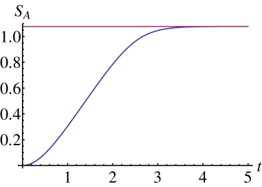
(a) Low effective temperature, $\kappa_{2}=1$

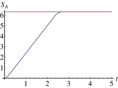
(b) High effective temperature, $\kappa_{2}=0.2$

Figure 1: Entanglement entropy growth of an interval(r=5) in CC state.

Taking the high temperature limit $\kappa_{2}\to 0$, we get the extensive thermal entropy formula $S_{therm}=\frac{1}{3}\frac{\pi r}{\beta}$.

Besides the thermalization, the most interesting aspect of figure (1) is that the entanglement entropy grows monotonically. The first derivative of $S_{A}$ w.r.t. time is

$$\left<\frac{\partial S_{A}}{\partial t}\right>_{CC} = \frac{\pi\sinh^{2}\left(\frac{\pi r}{4\kappa_{2}}\right)\tanh\left(\frac{\pi t}{2\kappa_{2}}\right)}{3\kappa_{2}\left[\cosh\left(\frac{\pi r}{2\kappa_{2}}\right)+\cosh\left(\frac{\pi t}{\kappa_{2}}\right)\right]}$$ (87)

$$= \frac{\pi}{12\kappa_{2}}\left[2\tanh\left(\frac{\pi t}{2\kappa_{2}}\right)-\tanh\left(\frac{\pi(r+2t)}{4\kappa_{2}}\right)+\tanh\left(\frac{\pi(r-2t)}{4\kappa_{2}}\right)\right]\$$ (88)

From the first expression, as a function of time $t>0$, it is clear that there are no finite zero. Hence, the EE growth of CC state is always monotonically increasing. Also note that in the high effective temperature limit $\kappa_{2}\to 0$, the approach to thermal value is sharper. In the limiting case, from the second expression, it is clear that the thermalization time is

$$t=\frac{r}{2}\$$ (89)

which has also been calculated using BCFT techniques in [6].

It would be interesting to check the monotonicity of EE growth in gCC states. Unfortunately, even for the free fermions with explicit twist operators, the entanglement entropy in gCC state with $W_{4}$ charge cannot be explicitly calculated. The bilinear fermionic $\mathcal{W}_{4}(w)$ current when bosonized gives $\phi^{4}$ terms[10], so the bosonized theory is an intereacting theory.

7 Non-Monotonic EE Growth and Dynamical Phase Transition

Although we could not calculate EE in gCC state with $W_{4}$ charge of the fermionic bilinear $\mathcal{W}_{4}$ current, we can still calculate entanglement entropy explicitly with the fermionic charge corresponding to the bosonic charge $W_{4}(w)=\sum_{k}|k|^{3}d^{\dagger}_{k}d_{k}$, where $d^{\dagger}_{k}$ and $d_{k}$ are the bosonic annihilation and creation operators. As mentioned above, the zero modes do not play any role. Refermionization of the bosonic bilinear $\mathcal{W}_{4}$ is done in Appendix F. So, the fermionic state that we are considering is

$$|\Psi\rangle=\text{e}^{-\kappa_{2}H_{f}-\kappa_{4}\tilde{W}_{4}}|D_{f}\rangle\$$ (90)

where the expression for $\tilde{W}_{4}$ is given in (137).

Again, the Rényi and entanglement entropies are given by the expression (77) and (78). The scalar propagator with the bosonic $W_{4}$ charge has also been calculated in MPS.

$$\langle\phi(0,t)\phi(r,t)\rangle=\int_{-\infty}^{\infty}\frac{dk}{8\pi}\frac{e^{ikr}}{k}\left[\coth\left(2k\left(\kappa_{2}+\kappa_{4}k^{2}\right)\right)-\cos(2kt){\rm cosech}\left(2k\left(\kappa_{2}+\kappa_{4}k^{2}\right)\right)\right]\$$ (91)

The momentum integral cannot be done explicitly. But we still can plot the entanglement entropy numerically. Figure (2) are the plots of EE growth with ‘small’ and ‘large’ values of $\kappa_{4}$. As expected, the entanglement entropy reaches an equilibrium quickly.

(a) Monotonic behavior, $\kappa_{4}=0.01$

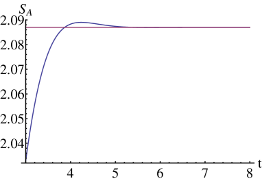
(b) Non-monotonic behaviour, $\kappa_{4}=0.30$

Figure 2: Entanglement entropy growth of an interval(r=5) for different choice of $\kappa_{4}$ and $\kappa_{2}=1$.

The most interesting aspect of Figure (2) is the non-monotonic growth of EE in the gCC state with ‘large’ $\kappa_{4}$. As in case of CC state, to study the monotonic or non-monotonic behaviour of $S_{A}$, the more appropriate quantity is not $S_{A}$ but rather $\frac{\partial S_{A}}{\partial t}$, the expression also simplifies tremendously.

$$\left<\frac{\partial S_{A}}{\partial t}\right>_{gCC} = \frac{1}{3}\int_{-\infty}^{\infty}\,dk\,(1-e^{ikr})\text{cosech}(2\kappa_{2}k+2\kappa_{4}k^{3})\sin(2kt)$$ (92)

$$= \frac{1}{3}\int_{-\infty}^{\infty}\,dk\,(1-\cos(kr))\text{cosech}(2\kappa_{2}k+2\kappa_{4}k^{3})\sin(2kt)\$$

Unfortunately, the above integral still cannot be done in closed form. The objective is to find finite positive real zeroes of the above expression as a function of time $t$. But, calculating zeroes of Fourier transforms, unless it can be done in closed form, is notoriously hard, the most famous example being the Riemann hypothesis.

The most interesting question that can be asked in Figure (2) is whether even a small infinitesimal $\kappa_{4}$, although not visible in the numerical plot, gives rise to the non-monotonic EE growth or whether the non-monotonic behaviour starts from a sharp finite value of $\kappa_{4}$. If it is the second case, then it is a dynamical phase transition. In other words, the question is whether (92) has finite zeroes as a function of time even for an infinitesimal $\kappa_{4}$ or do the finite zeroes appear for $\kappa_{4}$ greater than a critical value.

We found that the non-monotonic behaviour starts abruptly at a critical value of $\kappa_{4}=16\kappa_{2}^{3}/27\pi^{2}$, i.e., it is a dynamical phase transition. In terms of the effective temperature and chemical potential in the stationary limit, $\beta=4\kappa_{2}$ and $\mu_{4}=4\kappa_{4}$, the critical value is $\mu_{4}=\beta^{3}/27\pi^{2}$.

Althought the integral (92) cannot be done in closed form, we can take advantage of the fact that for our question we do not need to know the precise zeroes. Using contour integration, the integral is given by the sum of residues of the poles given by $2\kappa_{2}k+2\kappa_{4}k^{3}=in\pi$ where $n\in\mathbb{Z}-\{0\}$. $n=0$ is not a pole of (92). The expressions of the poles(from MPS) are

$$k_{1} = \frac{-2\ 6^{2/3}\kappa_{2}+\sqrt[3]{6}\left(\sqrt{48\kappa_{2}^{3}-81\pi^{2}\kappa_{4}n^{2}}+9i\pi\sqrt{\kappa_{4}}n\right)^{2/3}}{6\sqrt[3]{\sqrt{3}\sqrt{\kappa_{4}^{3}\left(16\kappa_{2}^{3}-27\pi^{2}\kappa_{4}n^{2}\right)}+9i\pi\kappa_{4}^{2}n}}$$ (93)

$$k_{2} = \frac{4\sqrt[3]{-6}\kappa_{2}+i\left(\sqrt{3}+i\right)\left(\sqrt{48\kappa_{2}^{3}-81\pi^{2}\kappa_{4}n^{2}}+9i\pi\sqrt{\kappa_{4}}n\right)^{2/3}}{2\ 6^{2/3}\sqrt[3]{\sqrt{3}\sqrt{\kappa_{4}^{3}\left(16\kappa_{2}^{3}-27\pi^{2}\kappa_{4}n^{2}\right)}+9i\pi\kappa_{4}^{2}n}}$$ (94)

$$k_{3} = -\frac{\sqrt[3]{-1}\left(2\sqrt[3]{-6}\kappa_{2}+\left(\sqrt{48\kappa_{2}^{3}-81\pi^{2}\kappa_{4}n^{2}}+9i\pi\sqrt{\kappa_{4}}n\right)^{2/3}\right)}{6^{2/3}\sqrt{\kappa_{4}}\sqrt[3]{\sqrt{48\kappa_{2}^{3}-81\pi^{2}\kappa_{4}n^{2}}+9i\pi\sqrt{\kappa_{4}}n}}\$$ (95)

Out of the three poles, only one is perturbative. In $\kappa_{4}\to 0$ series expansion, the other two start with $\mathcal{O}(\frac{1}{\sqrt{\kappa_{4}}})$. One of the three poles is always imaginary for arbitrary $n$ and arbitrary positive $\kappa_{4}$.

There are three important ingredients for the proof of the dynamical phase transition:

1. All three $n^{\text{th}}$ poles become purely imaginary when $16\kappa_{2}^{3}-27\pi^{2}\kappa_{4}n^{2}$ is negative, or $\kappa_{4}$ is greater than $16\kappa_{2}^{3}/27\pi^{2}n^{2}$, we will call this the $n^{\text{th}}$ critical value $\kappa_{4c,n}$,

   $$\kappa_{4c,n} =\frac{16\kappa_{2}^{3}}{27\pi^{2}n^{2}}\$$ (96)

   Below this value, the residues of the $n^{\text{th}}$ poles are exponential decaying functions of time $t$, with no oscillatory factor. Obviously, ($n=\pm 1$) critical value $\kappa_{4c}$ is larger than $\kappa_{4c,n}$ for $|n|>1$. With $\kappa$ scaled to $1$, $\kappa_{4c}$ is $16\kappa_{2}^{3}/27\pi^{2}\sim 0.0600422$.

2. With $\kappa_{4}$ less than $(n=\pm 1)$ critical value, the sum of the residues of ($n=\pm 1$) poles is larger than the sum of the residues of all the other ($|n|>1$) poles. Hence, the behaviour of the first poles of $n=\pm 1$ dictate the behaviour of the integral (92) when $\kappa_{4}<16\kappa_{2}^{3}/27\pi^{2}$.

3. Above this critical value, for each $n$, two of the poles have real parts while one of them, say $k_{1}$, is imaginary. The poles are

   $$k_{1}=-2i\,\text{sgn}(n)\,b,\qquad k_{2}=a+i\,\text{sgn}(n)\,b,\qquad k_{3}=-a+i\,\text{sgn}(n)\,b$$ (97)

   $$a=\frac{B^{2/3}-2\sqrt[3]{6}\kappa_{2}}{2\ 2^{2/3}\sqrt[6]{3}\sqrt[3]{B}\sqrt{\kappa_{4}}},\qquad b=\frac{B^{2/3}+2\sqrt[3]{6}\kappa_{2}}{2\ 6^{2/3}\sqrt[3]{B}\sqrt{\kappa_{4}}}$$

   $$B=\sqrt{81\pi^{2}\kappa_{4}n^{2}-48\kappa_{2}^{3}}+9\pi|n|\sqrt{\kappa_{4}}\$$

   where we have to take the real roots of the radicals. $k_{1}$’s have the largest imaginary parts and the exponential decay of their residues as a function of time are faster while the other poles $k_{2}$ and $k_{3}$ have comparatively large magnitudes and ocsillations. In the total integral, the contributions of the imaginary poles $k_{1}$’s cannot compete with the contributions of the oscillating poles. Lastly, it would be a very special arrangment if all ocsillating terms conspire to give a non-oscillatory sum. Hence, the total integral is oscillatory as a function of time and the EE growth is non-monotonic.

For future reference, we also note that the expansion of the real part ‘$a$’ in (97) around the $n^{\text{th}}$ critical value $\kappa_{4c,n}$ is

$$a=\frac{\sqrt[3]{\pi}\sqrt[3]{|n|}\sqrt{\kappa_{4}-\kappa_{4c,n}}}{2^{2/3}\sqrt{3}\kappa_{4c,n}^{5/6}}-\frac{35\left(\sqrt[3]{\pi}\sqrt[3]{|n|}\right)(\kappa_{4}-\kappa_{4c,n})^{3/2}}{54\left(2^{2/3}\sqrt{3}\kappa_{4c,n}^{11/6}\right)}\\ +\frac{1001\sqrt[3]{\pi}\sqrt[3]{|n|}(\kappa_{4}-\kappa_{4c,n})^{5/2}}{1944\ 2^{2/3}\sqrt{3}\kappa_{4c,n}^{17/6}}+\mathcal{O}(\kappa_{4}-\kappa_{4c,n})^{7/2}$$ (98)

For all our calculations below, we have scaled $\kappa_{2}$ to be 1. The first point is clear from figure (3). The real parts of ($n=\pm 1$) poles vanish at $\kappa_{4}\sim 0.060$, which is the critical value found above. The critical value of $(n=\pm 2$) poles is $\kappa_{4}\sim 0.015$.

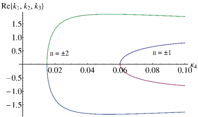
Figure 3: Real parts of poles of $n\in\{\pm 1,\pm 2\}$ as a function of $\kappa_{4}$ with $\kappa_{2}$ scaled to $1$.

Below the critical value, we will show that the total contributions from $n=\pm 1$ poles is larger than the sum of all residues of $|n|>1$ poles. We will concentrate on the late time period, $t>r/2$. For $e^{i2kt}$ of $\sin(2kt)$ factor in (92), the contour is closed upward encircling the upper half plane, and for $e^{-i2kt}$, the contour is closed downward encircling the lower half plane. From the expansion of ${\rm cosech}\left(2\kappa_{4}\left(k-k_{1}\right)\left(k-k_{2}\right)\left(k-k_{3}\right)+i\pi n\right)$ around $k_{1}$, the contribution from $k_{1}$ poles for arbitrary $n$ are the real parts of

$$P_{n}(k_{1}) =2\pi iR_{1}(k_{1})=\frac{(-1)^{n}}{6\kappa_{4}(k_{1}-k_{2})(k_{1}-k_{3})}\,\left(e^{i2k_{1}t}-\frac{e^{ik_{1}(r+2t)}+e^{ik_{1}(-r+2t)}}{2}\right)\; \text{if}\;\text{Im}[k_{1}]>0$$

$$Q_{n}(k_{1}) =-2\pi iR_{2}(k_{1})=\frac{(-1)^{n}}{6\kappa_{4}(k_{1}-k_{2})(k_{1}-k_{3})}\,\left(e^{-i2k_{1}t}-\frac{e^{ik_{1}(r-2t)}+e^{-ik_{1}(r+2t)}}{2}\right)\; \text{if}\;\text{Im}[k_{1}]<0$$

where $R_{1}$ and $R_{2}$ denote the residues. Similarly, cyclic replacements of $k_{1}$ with $k_{2}$ and $k_{3}$ give the contributions of $k_{2}$ and $k_{3}$ poles. For the poles in the lower half of the complex plane, since the contour is anticlockwise, $Q_{n}$ have an extra minus sign in the residue. We will call the contributions to the integral form $n=\pm 1$ poles as $I_{0}(t)$ and the contributions of the $|n|>1$ poles as $I_{1}(t)$. The other parameters ($\kappa_{4}$, $r$ and $\kappa$ which is already scaled to 1) are suppressed.

As a first visual evidence, Figure (4) is the comparison of numerical integration of (92) and $I_{0}(t)$. It is evident that the residues of ($n=\pm 1$) poles dominate the contour integration. We have chosen $\kappa_{4}=0.0600420$ which is very close to the critical value. As mentioned above, with this choice, all the poles except the $n=\pm 1$ poles give ocsillating residues as a function of time. Although it is not very conspicuous, it is also evident from the graph that $I_{1}(t)$ is oscillating around $I_{0}(t)$, the value of the numerical integration is above the $I_{0}(t)$ curve in some regions and below in other regions of time $t$.

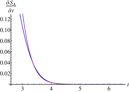
Figure 4: Comparison of numerical integration of $\left<\partial{S_{A}}/\partial t\right>_{gCC}$ (blue curve) and $I_{0}(t)$ (purple curve) as a function of time $t$. The parameters are $\kappa_{4}=0.0600420$, $r=5$.

The numerical integration is unreliable in the long time limit. So, to complete our argument, we will calculate an upper bound of $I_{1}(t)$ and compare it with $I_{0}(t)$ for a specific time $t$. The choice of the parameters are

$$\kappa=1,\;\kappa_{4}=0.0600420,\;r=5,\;t=4r=20,\$$ (101)

With these parameters, the $n=1$ and $n=-1$ poles are

$$k_{1} =2.3538234i k_{2} =2.3585719i k_{3} =-4.7123954i ;\;n =1$$ (102)

$$k_{1} =4.7123954i k_{2} =-2.3538234i k_{3} =-2.3585719i ;\;n =-1\$$ (103)

and $I_{0}(t)$ is given by

$$I_{0}(t)|_{t=20} = P(k_{1})|_{n=1}+P(k_{2})|_{n=1}+Q(k_{3})|_{n=1}+P(k_{1})|_{n=-1}+Q(k_{2})|_{n=-1}+Q(k_{3})|_{n=-1}$$ (104)

$$= 6.646589\times 10^{-35}\$$

We can show that $I_{1}(t)|_{t=20}$ is less than $I_{0}(t)|_{t=20}$. The first few poles are

$$k_{1} =5.5495551i k_{2} =2.5383386-2.7747775i k_{3} =-2.5383386-2.7747775i ;\;n =-3$$

$$k_{1} =5.1737935i, k_{2} =1.8496206-2.5868967i k_{3} =-1.8496206-2.5868967i ;\;n =-2$$

$$k_{1} =-5.1737935i k_{2} =-1.8496206+2.5868967i k_{3} =1.8496206+2.5868967i ;\;n =2$$

$$k_{1} =-5.54955505i k_{2} =-2.5383386+2.7747775i k_{3} =2.5383386+2.7747775i ;\;n =3\$$

The residues of these ($|n|>1$) poles cannot be summed up into a closed form, as that would amount to doing the integral in closed form. We are interested in an upper bound. The residues of two of the three poles of every ($|n|>1$) have an oscillation factor. As we saw, even each residue has a separate 3-6 real oscillating terms as a function of time. So, we can represent the sum of the modulus (absolute value of the amplitude) of the oscillating terms of the three residues for each $n$, by a bigger function which has the analytic sum from $|n|>1$ to infinity. And if the sum is less $I_{0}(t)$, then $I_{0}(t)$ dominates the contribution from all the other poles.

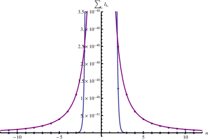
Figure 5: Comparison of sum of modulus of residues of ($|n|>1$) poles with the approximating function $f(n)=10^{-39}/n^{2}$. The dots are the discrete $n$ values of the corresponding functions.

Figure (5) are the plots of the sum of the moduli separately for the oscillating terms of the three residues as a function of $n$ and the approximating function $f(n)=10^{-39}/n^{2}$. Now, we have

$$\sum_{-\infty}^{n=-2}\frac{10^{-39}}{n^{2}}+\sum_{n=2}^{\infty}\frac{10^{-39}}{n^{2}}=1.289868\times 10^{-39}\$$ (105)

This is much less than $I_{0}(t)|_{t=20}$ in (104) and is of the order of $10^{-5}$ of $I_{0}(t)|_{t=20}$. So, the non-oscillating $I_{0}(t)$ dominates $I_{1}(t)$, the contribution from the other poles. Hence, below $\kappa_{4}=16\kappa_{2}^{3}/27\pi^{2}$, the EE growth is monotonic.

Visually from figure (4), $t=3.7$ is a time-slice where the difference between $I_{0}(t)$ and the numerical integration has a local maxima. At this time slice, repeating the above exercise, $I_{0}(t)|_{t=3.7}=0.109727$ and repeating the same exercise of estimating the upper bound of $I_{1}(t)|_{t=3.7}$ with the same parameters as (101) except the change in $t$, we get a good upper bound to be $0.0064493$ which is less than $I_{0}(t)|_{t=3.7}$ and is of the order of $60\%$ of $I_{0}(t)|_{t=3.7}$. So, the approximation of the full integral by $I_{0}(t)$ gets better with increasing time. In the long time limit, we can effectively take the only time-dependence to be the time-dependence of $I_{0}(t)$. It is worth mentioning here that even $(n=\pm 1)$ pole calculations take into account $\kappa_{4}$ non-perturbatively, since two of the poles of each $n$ are non-perturbative in $\kappa_{4}$.

As listed above as one of the main points, above the critcal value, each $n$ has an imaginary pole but the other two poles have real parts and also have larger magnitudes so the total residue of the three poles of each $n$ is oscillatory. It would also be a very special arrangement if all the oscillatory contributions of each $n$ conspire to give a non-oscillatory $\partial S_{A}/\partial t$. Hence, we conclude that the EE growth is non-monotonic above the critical value.

Near the critical point $(\kappa_{4}-\kappa_{4c})\to 0^{+}$, we can try to estimate an upper bound of the time upto which the EE growth is monotonic. The upper bound is half of the longest time period. Using the leading term in expansion of ‘$a$’ from (98) and the expressions of the residues (LABEL:I1) and (LABEL:I2), the lowest frequency($|n|=1$) gives the upper bound as

$$\frac{\sqrt[3]{\pi}\sqrt{\kappa_{4}-\kappa_{4c}}}{2^{2/3}\sqrt{3}\kappa_{4c}^{5/6}}(2t-r)=\pi\quad\Rightarrow\quad t=\frac{(2\pi)^{2/3}\sqrt{3}\kappa_{4c}^{5/6}}{2\sqrt{\kappa_{4}-\kappa_{4c}}}+\frac{r}{2}\;\sim\;\frac{2.95\,\kappa_{4c}^{5/6}}{\sqrt{\kappa_{4}-\kappa_{4c}}}\$$ (106)

where finite ‘$r$’ can be neglected in the limit $(\kappa_{4}-\kappa_{4c})\to 0^{+}$.

The critical value in terms the effective temperature $\beta=4\kappa_{2}$ and chemical potential $\mu_{4}=4\kappa^{4}$ in the stationary limit is

$$\mu_{4}=\frac{\beta^{3}}{27\pi^{2}}\$$ (107)

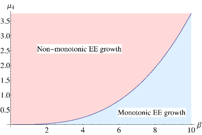
Figure 6: The critical curve $\mu_{4}=\beta^{3}/27\pi^{2}$ in terms of the effective temperature and chemical potential in the stationary limit and the phase diagram.

For the early times $t<r/2$, in the residue calculations (LABEL:I1) and (LABEL:I2), we have to replace the sign of the exponents with $r-2t$ so the magnitudes of the exponentials decreases as time increases. Upto the critical value of $\kappa_{4}$, the EE growth is always monotonic for this time period.

7.1 Turning on other charges

We could also calculate the EE growth of gCC states with other charges of the fermionic theory corresponding to bosonic bilinear $W_{2n}=\sum|k|^{2n-1}d^{\dagger}_{k}d_{k}$ where $n=3,4,5,...$. Repeating the exercise of quenching tuned squeezed states of scalar field theory in MPS, the propagator with these charges are simply given by

$$\langle\phi(0,t)\phi(r,t)\rangle=\int\frac{dk}{4\pi}\frac{e^{ikr}}{k}\left(\coth\left(2\kappa_{2}k+\sum_{n=2}^{\infty}\kappa_{2n}k^{2n-1}\right)\right.\\ \left.-\cos(2kt){\rm cosech}\left(2\kappa_{2}k+\sum_{n=2}^{\infty}\kappa_{2n}k^{2n-1}\right)-1\right)$$ (108)

Substituting this propagator in the general formula (77) and (78) give the Rényi entropy and entanglement entropy. The first derivative of EE w.r.t. time is

$$\left<\frac{\partial S_{A}}{\partial t}\right>_{gCC}=\frac{1}{3}\int_{-\infty}^{\infty}\,dk\,(1-\cos(kr))\text{cosech}\left(2\kappa k+\sum_{n=2}^{\infty}\kappa_{2n}k^{2n-1}\right)\sin(2kt)\$$ (109)

We believe the dynamics will be much richer with these other charges, with much more complex phase diagrams which can be in a $n-1$ dimensional space. But the general poles analysis cannot be done in these cases because the poles will be given by quintic and higher order equations. Considering gCC states with $W_{4}$ and $W_{6}$ charges, the numerical plots of EE growth looks the same as (2) where by trial and error method, some parameter subspace gives monotonic growth and some subspaces do not give monotonic growth. Considering $n=\pm 1$, the poles are given by $2\kappa_{2}k+2\kappa_{4}k^{3}+2\kappa_{6}k^{5}=i\pi$. For $\kappa_{2}=1$ and $\kappa_{4}=0.06$, numerically we find two interesting parameter subspaces of $\kappa_{6}$. The first one is when all the poles become imaginary when $\kappa_{4}$ is decreased.

$$k_{1}=2.0887597\,\text{sgn}(n)\,i,\quad k_{2}=2.9527785\,\text{sgn}(n)\,i,\quad k_{3}=-6.5425830\,\text{sgn}(n)\,i,$$

$$k_{4}=-6.6158300\,\text{sgn}(n)\,i,\quad k_{5}=8.1168748\,\text{sgn}(n)\,i\qquad\text{for}\qquad\kappa_{6}=0.0007249$$ (110)

$$k_{1}=-0.0076887-6.5788763\,\text{sgn}(n)\,i,\quad k_{2}=2.0887456\,\text{sgn}(n)\,i,\quad k_{3}=2.9528549\,\text{sgn}(n)\,i,$$

$$k_{4}=8.1161520\,\text{sgn}(n)\,i,\quad k_{5}=0.0076887-6.5788763\,\text{sgn}(n)\,i\qquad\text{for}\qquad\kappa_{6}=0.0007250\$$ (111)

This looks like the same transition if $n=\pm 1$ dominates, but the poles with real parts have large imaginary part also, so they would be highly damped. The other case is

$$k_{1}=-0.8215058+1.9681831\,\text{sgn}(n)\,i,\quad k_{2}=-5.2389645\,\text{sgn}(n)\,i,\quad k_{3}=-5.2472000\,\text{sgn}(n)\,i,$$

$$k_{4}=6.5497983\,\text{sgn}(n)\,i,\quad k_{5}=0.8215058+1.9681831\,\text{sgn}(n)\,i\qquad\text{for}\qquad\kappa_{6}=0.0019179$$ (112)

$$k_{1}=-0.8215060+1.9681836\,\text{sgn}(n)\,i,\quad k_{2}=-0.0040372-5.2430724\,\text{sgn}(n)\,i,$$

$$k_{3}=6.5497775\,\text{sgn}(n)\,i,\quad k_{4}=0.0040372-5.2430724\,\text{sgn}(n)\,i,$$

$$k_{5}=0.8215060+1.9681836\,\text{sgn}(n)\,i\qquad\text{for}\qquad\kappa_{6}=0.0019180\$$ (113)

for the smaller $\kappa_{4}$, although two of the poles have real parts, they have to compete with the three imaginary poles. So, this could also be phase transition.

8 Discussion

In this paper, we have examined free fermionic mass quench. We find that the ground state quench equilibrates but not to a thermal ensemble. Starting from specially prepared squeezed states, we get CC and gCC states with fermionic bilinear $W_{2n}$ charges. Calculation of correlators in CC and gCC states explicitly shows thermalization to thermal emsemble and GGE respectively.

For CC state, we calculate EE growth exactly. The EE growth is strictly monotonically increasing. For gCC state with a particular charge, we find dynamical phase transition in which the EE growth is monotonic upto a critical value of the effective chemical potential. In the pure state, the effective chemical potential is the coupling constant of the current corresponding to the charge. Above the critical value, the EE growth is non-monotonic. It would be interesting to reproduce our result in large $c$ holographic CFTs and examine what it would mean for Black hole physics.

Appendix A Conventions

$$\eta_{\mu\nu}=\begin{bmatrix}1&0\\ 0&-1\end{bmatrix},\quad\partial_{\mu}=(\partial_{t},\partial_{x}),\quad\gamma^{\mu}\partial_{\mu}=\gamma^{0}\partial_{t}-\gamma^{1}\partial_{x},$$

$$w=t-x,\quad\bar{w}=t+x,\quad\partial=\frac{\partial}{\partial w}=\frac{1}{2}\left(\frac{\partial}{\partial t}-\frac{\partial}{\partial x}\right),\quad\bar{\partial}=\frac{\partial}{\partial\bar{w}}=\frac{1}{2}\left(\frac{\partial}{\partial t}+\frac{\partial}{\partial x}\right)$$

$$\gamma^{0}_{d}=\begin{bmatrix}1&0\\ 0&-1\end{bmatrix},\quad\gamma^{1}_{d}=\begin{bmatrix}0&1\\ -1&0\end{bmatrix},\quad\text{in Dirac basis}.$$

$$S=\frac{1}{\sqrt{2}}\begin{bmatrix}1&-1\\ 1&1\end{bmatrix},\gamma^{0}_{c}=S\gamma^{0}_{d}S^{-1}=\begin{bmatrix}0&1\\ 1&0\end{bmatrix},\quad\gamma^{1}_{c}=S\gamma^{1}_{d}S^{-1}=\begin{bmatrix}0&1\\ -1&0\end{bmatrix},\quad\text{in chiral basis.}$$

$$\left\{a_{k},a^{\dagger}_{k^{\prime}}\right\}=2\pi\,\delta(k-k^{\prime}),\quad\left\{b_{k},b^{\dagger}_{k^{\prime}}\right\}=2\pi\,\delta(k-k^{\prime}),\,\text{other anticommutators are zero.}$$

$$\left\{a_{n},a^{\dagger}_{n^{\prime}}\right\}=\delta(n-n^{\prime}),\quad\left\{b_{n},b^{\dagger}_{n^{\prime}}\right\}=\delta(n-n^{\prime}),\,\text{other anticommutators are zero.}\$$

We will use $k=\frac{2\pi n}{L}$ for continuum limit($L\to\infty$) and $n$ for quantization in a finite box of size L, where $n=n^{\prime}+1/2$ and $n^{\prime}\in\mathbb{Z}$.

Appendix B Spinors and transformation to chiral basis:

Taking constant mass $m$, we can easily find the boosted spinors, $u(k,m)$ and $v(k,m)$. For constant $m$, $\phi_{+p}(t)=e^{-i\omega t}$ and $\phi_{-m}(t)=e^{i\omega t}$. So from (4),

$$U(x,t) = \left[\gamma^{0}\partial_{t}-\gamma^{1}\partial_{x}-im\right]e^{-i\omega t+ikx}\begin{bmatrix}1\\ 0\end{bmatrix}=i\begin{bmatrix}-(\omega+m)\\ k\end{bmatrix}e^{-ik\cdot x}$$

$$V(x,t) = \left[\gamma^{0}\partial_{t}-\gamma^{1}\partial_{x}-im\right]\begin{bmatrix}0\\ 1\end{bmatrix}e^{ik\cdot x}=i\begin{bmatrix}k\\ -(\omega+m)\end{bmatrix}e^{ik\cdot x}\$$

Hence, upto normalizations fixed by inner products, the boosted spinors are

$$u(k,m)=i\begin{bmatrix}-(\omega+m)\\ k\end{bmatrix},\quad v(k,m)=i\begin{bmatrix}k\\ -(\omega+m)\end{bmatrix}\$$

We have the adjoint spinors as,

$$\bar{u}(k,m) = u^{\dagger}(k,m)\gamma^{0}=-i\begin{bmatrix}-(\omega+m)&k\end{bmatrix}\begin{bmatrix}1&0\\ 0&-1\end{bmatrix}=i\begin{bmatrix}-(\omega+m)&-k\end{bmatrix}$$

$$\bar{v}(k,m) = v^{\dagger}(k,m)\gamma^{0}=-i\begin{bmatrix}k&-(\omega+m)\end{bmatrix}\begin{bmatrix}1&0\\ 0&-1\end{bmatrix}=i\begin{bmatrix}k&(\omega+m)\end{bmatrix}\$$

Now borrowing Peskin & Schroeder(P&S) conventions of spinors, we want to fix the inner products $\bar{u}(k,m)u(k,m)=2m$ and $\bar{v}(k,m)v(k,m)=-2m$,

$$\bar{u}(k,m)u(k,m) = \begin{bmatrix}-(\omega+m)&-k\end{bmatrix}\begin{bmatrix}-(\omega+m)\\ k\end{bmatrix}=2m(\omega+m)$$

$$\bar{v}(k,m)v(k,m) = \begin{bmatrix}k&(\omega+m)\end{bmatrix}\begin{bmatrix}k\\ -(\omega+m)\end{bmatrix}=-2m(\omega+m)\$$

So the normalized spinors are

$$u(k,m) = \frac{1}{\sqrt{(\omega+m)}}\begin{bmatrix}(\omega+m)\\ -k\end{bmatrix},\quad v(k,m)=\frac{1}{\sqrt{(\omega+m)}}\begin{bmatrix}k\\ -(\omega+m)\end{bmatrix}$$

$$\bar{u}(k,m) = \frac{1}{\sqrt{(\omega+m)}}\begin{bmatrix}(\omega+m)&k\end{bmatrix},\quad\bar{v}(k,m)=\frac{1}{\sqrt{(\omega+m)}}\begin{bmatrix}k&(\omega+m)\end{bmatrix}$$

The spinors with time-dependent mass $m(t)$ are obtained by just substituting $m(t)$ in the place of ‘$m$’ only inside the matrices, which is clearly seen from (12) and (13). The normalization cannot be changed to time-dependent mass else the spinors won’t be solutions of the corresponding Dirac equation.

The transformation to chiral basis is accomplished by using the transformation matrix $S=\frac{1}{\sqrt{2}}\begin{bmatrix}1&-1\\ 1&1\end{bmatrix}$. The mode expansion as in P&S is

$$\Psi(x,t) = \int\frac{dk}{2\pi}\frac{1}{\sqrt{2\omega}}\left[a_{k}u(k,m)e^{-ik\cdot x}+b^{\dagger}_{k}v(k,m)e^{ik\cdot x}\right]$$

$$= \int\frac{dk}{2\pi}\frac{1}{\sqrt{2\omega}}\left[a_{k}\frac{1}{\sqrt{(\omega+m)}}\begin{bmatrix}(\omega+m)\\ -k\end{bmatrix}e^{-ik\cdot x}+b^{\dagger}_{k}\frac{1}{\sqrt{(\omega+m)}}\begin{bmatrix}k\\ -(\omega+m)\end{bmatrix}e^{ik\cdot x}\right]$$

$$\xrightarrow{m\to 0} \int\frac{dk}{2\pi}\frac{1}{\sqrt{2}}\left[a_{k}\begin{bmatrix}1\\ -\text{sgn}(k)\end{bmatrix}e^{-ik\cdot x}+b^{\dagger}_{k}\begin{bmatrix}\text{sgn}(k)\\ -1\end{bmatrix}e^{ik\cdot x}\right]$$

$$= \int\frac{dk}{2\pi}\frac{1}{\sqrt{2}}\begin{bmatrix}a_{k}e^{-ik\cdot x}+\text{sgn}(k)b^{\dagger}_{k}e^{ik\cdot x}\\ -\text{sgn}(k)a_{k}e^{-ik\cdot x}-b^{\dagger}_{k}e^{ik\cdot x}\end{bmatrix}\$$

In the chiral basis,

$$\Psi_{c}(x,t) = S\cdot\Psi(x,t)=\frac{1}{\sqrt{2}}\begin{bmatrix}1&-1\\ 1&1\end{bmatrix}\cdot\int\frac{dk}{2\pi}\frac{1}{\sqrt{2}}\begin{bmatrix}a_{k}e^{-ik\cdot x}+\text{sgn}(k)b^{\dagger}_{k}e^{ik\cdot x}\\ -\text{sgn}(k)a_{k}e^{-ik\cdot x}-b^{\dagger}_{k}e^{ik\cdot x}\end{bmatrix}$$ (115)

$$= \int_{-\infty}^{\infty}\frac{dk}{2\pi}\frac{1}{2}\begin{bmatrix}(1+\text{sgn}(k))(a_{k}e^{-ik\cdot x}+b^{\dagger}_{k}e^{ik\cdot x})\\ (1-\text{sgn}(k))(a_{k}e^{-ik\cdot x}-b^{\dagger}_{k}e^{ik\cdot x})\end{bmatrix}\$$

Writing this as $\psi(x,t)$ and $\bar{\psi}(x,t)$,

$$\psi(x,t) = \int_{0}^{\infty}\frac{dk}{2\pi}(a_{k}e^{-ik\cdot x}+b^{\dagger}_{k}e^{ik\cdot x})$$ (116)

$$\bar{\psi}(x,t) = \int_{-\infty}^{0}\frac{dk}{2\pi}(a_{k}e^{-ik\cdot x}-b^{\dagger}_{k}e^{ik\cdot x})\$$ (117)

Appendix C Fermionic Boundary State

The action (1) with $m(t)=0$ in the chiral basis is

$$S =-\int dx^{2}\,\left[i\bar{\Psi}\gamma^{\mu}\partial_{\mu}\Psi+\Psi\gamma^{\mu}\partial_{\mu}\bar{\Psi}\right]$$

$$=-\frac{i}{2}\int dwd\bar{w}\left(\psi^{\dagger}\bar{\partial}\psi+\bar{\psi}^{\dagger}\partial\bar{\psi}+\psi\bar{\partial}\psi^{\dagger}+\bar{\psi}\partial\bar{\psi}^{\dagger}\right)\$$

On varying the action and collecting terms, we get the following

$$\delta S=\int d^{2}x\left(\delta\psi^{\dagger}\bar{\partial}\psi+\delta\psi\bar{\partial}\psi^{\dagger}+\delta\bar{\psi}^{\dagger}\partial\bar{\psi}+\delta\bar{\psi}\partial\bar{\psi}^{\dagger}\right)$$ (118)

Given a boundary at $t=0$, it will also have certain boundary terms, which we want to be zero.

$$\left.\psi^{\dagger}\delta\psi+\psi\delta\psi^{\dagger}+\bar{\psi}^{\dagger}\delta\bar{\psi}+\bar{\psi}\delta\bar{\psi}^{\dagger}\right|_{t=0}=0$$ (119)

We impose this as an operator equation on the boundary state $\left|B\right>$. The condition for a boundary state can be achieved via two identifications

$$\psi=i\bar{\psi}^{\dagger},\quad\text{and}\quad\psi^{\dagger}=i\bar{\psi}$$ (120)

$$\psi=-\bar{\psi},\quad\text{and}\quad\psi^{\dagger}=\bar{\psi}^{\dagger}\$$ (121)

Now we impose the boundary conditions at $t=0$ in terms of the mode expansions (116) and (117):

1. The boundary condition of (120) gives $a_{k}\mp ia_{-k}^{\dagger}=0$ for $k>0$ and $b_{k}\mp ib_{-k}^{\dagger}=0$ for $k<0$. Similarly, the second condition is $a_{k}\pm ia_{-k}^{\dagger}=0$ for $k<0$ and $b_{k}\pm ib_{-k}^{\dagger}=0$ for $k>0$. Combining the separate conditions, we get $a_{k}\mp i\,\text{sgn}(k)a^{\dagger}_{-k}=0$ and $b_{k}\pm i\,\text{sgn}(k)b_{-k}^{\dagger}=0$. Hence, the boundary state corresponding to the first identification is

   $$\left|N\right>=\exp\left(\sum\limits_{k}\ i\operatorname{sgn}(k)(a^{\dagger}_{k}a^{\dagger}_{-k}-b^{\dagger}_{k}b^{\dagger}_{-k})\right)\left|0\right>$$ (122)

2. The boundary condition (121) is $a_{k}\mp\text{sgn}(k)b_{-k}^{\dagger}=0$ for $k>0$, $a_{k}\pm b_{-k}^{\dagger}=0$ for $k<0$ and $b_{k}\pm a_{-k}^{\dagger}=0$ for $k<0$ and $b_{k}\mp a_{-k}^{\dagger}=0$ for $k>0$. The boundary state for the first identification is

   $$\left|D\right>=\exp\left(\sum\limits_{k}\operatorname{sgn}(k)a^{\dagger}_{k}b^{\dagger}_{-k}\right)\left|0\right>$$ (123)

From the action $S$, we can find the non-zero components of the energy-momentum tensor $T=T_{ww}$ and $\bar{T}=T_{\bar{w}\bar{w}}$, and the components of the $U(1)$ current are $J_{w}=J$ and $J_{\bar{w}}=\bar{J}$,

$$T=\frac{i}{2}\left(\psi^{\dagger}\partial\psi+\psi\partial\psi^{\dagger}\right) \bar{T} =\frac{i}{2}\left(\bar{\psi}^{\dagger}\bar{\partial}\bar{\psi}+\bar{\psi}\bar{\partial}\bar{\psi}^{\dagger}\right)$$ (124)

$$J=\psi^{\dagger}\psi \bar{J} =\bar{\psi}^{\dagger}\bar{\psi}\$$ (125)

The boundary conditions (120) and (121) satisfy the condition

$$T(w)|_{t=0} =\bar{T}(\bar{w})|_{t=0},\qquad\text{on the cylinder.}$$ (126)

$$\text{or},\quad\left(z^{2}T_{zz}(z)\right)|_{z(t=0)} =\left(\bar{z}^{2}\bar{T}_{\bar{z}\bar{z}}(\bar{z})\right)|_{\bar{z}(t=0)},\qquad\text{on the plane.}\$$ (127)

where $z=e^{2\pi(t-ix)/L}$ and $\bar{z}=e^{2\pi(t+ix)/L}$. Thus $\left|N\right>$ and $\left|D\right>$ are conformal invariant boundary states. It is also worth noting that the boundary conditions also satisfy

$$J(w)|_{t=0} =-\bar{J}(\bar{w})|_{t=0},\qquad\text{on the cylinder.}$$ (128)

$$\text{or},\quad\left(zJ_{z}(z)\right)|_{z(t=0)} =\left(\bar{z}\bar{J}_{\bar{z}}(\bar{z})\right)|_{\bar{z}(t=0)},\qquad\text{on the plane.}\$$ (129)

Considering the zero modes in the cylinder, it means that the above boundary states are not charged. With $Q=J_{0}+\bar{J}_{0}$,

$$Q|N\rangle=0,\qquad Q|D\rangle=0\$$ (130)

Besides, specially for the state $|D\rangle$, $(J_{0}-\bar{J}_{0})|D\rangle=0$. Hence

$$J_{0}|D\rangle=0\qquad\bar{J}_{0}|D\rangle=0\$$ (131)

Appendix D Bosonised Boundary State

Consider a Dirichlet boundary state $\varphi\left|D\right>=-\bar{\varphi}\left|D\right>$. Using the bosonised fermions :

$$\psi =e^{-i\frac{\sqrt{\pi}}{4}\bar{P}}:e^{-i\sqrt{4\pi}\varphi(w)}: \psi^{\dagger} =e^{i\frac{\sqrt{\pi}}{4}\bar{P}}:e^{i\sqrt{4\pi}\varphi(w)}:$$

$$\bar{\psi} =e^{-i\frac{\sqrt{\pi}}{4}P}:e^{i\sqrt{4\pi}\bar{\varphi}(\bar{w})}: \bar{\psi}^{\dagger} =e^{i\frac{\sqrt{\pi}}{4}P}:e^{-i\sqrt{4\pi}\bar{\varphi}(\bar{w})}:\$$

To translate the boson Dirichlet condition into the fermionic one, we get

$$\psi\left|D\right> = e^{-i\frac{\sqrt{\pi}}{4}\bar{P}}:e^{-i\sqrt{4\pi}\varphi}:|D\rangle$$

$$= e^{-\frac{\pi}{2}[Q,P]}e^{-i\frac{\sqrt{\pi}}{4}\bar{P}}e^{-i\frac{\sqrt{\pi}}{4}P}:e^{-i\sqrt{4\pi}\varphi}:\left|D\right>$$

$$= e^{-\frac{\pi}{2}[Q,P]}e^{-i\frac{\sqrt{\pi}}{4}\bar{P}}e^{-i\frac{\sqrt{\pi}}{4}P}:e^{i\sqrt{4\pi}\bar{\varphi}}:\left|D\right>$$

$$= e^{\frac{\pi}{2}([Q,P]-[\bar{P},\bar{Q}])}\ \bar{\psi}\left|D\right>$$

$$= e^{-i\pi}\ \bar{\psi}\left|D\right>=-\bar{\psi}\left|D\right>\$$

where we have used the relation $e^{x}\,e^{y}=e^{y+[x,y]+...}\,e^{x}$ and $[Q,P]=[\bar{Q},\bar{P}]=i$. We have also used (131) which gives $P|D\rangle=J_{0}|D\rangle=0$ and $\bar{P}|D\rangle=\bar{J}_{0})|D\rangle=0$.

Similarly, we can show that $(\psi^{\dagger}-\bar{\psi}^{\dagger})\left|D\right>$, $(\psi-i\bar{\psi}^{\dagger})\left|N\right>$ and $(\psi^{\dagger}-i\bar{\psi})\left|N\right>$ vanish, where $\left|N\right>$ is defined by $(\varphi-\bar{\varphi})\left|N\right>=0$ which is the Neumann boundary condition for scalar fields.

Appendix E Baker-Campbell-Hausdorff(BCH) formula

Although we are interested in the ‘out’ massless oscillators, the BCH formula is valid for both massive and massless oscillators. So, we will suppress the ‘in’ or ‘out’ identification of the oscillators. Starting from

$$|\Psi\rangle=\exp\left(\sum_{k}\text{sgn}(k)\gamma(k)a^{\dagger}_{k}b^{\dagger}_{-k}\right)|0\rangle\$$ (132)

we wish to obtain an expression of the form

$$\left|\psi\right>=\exp\left(-\sum\limits_{k}\kappa(k)(a^{\dagger}_{k}a_{k}+b^{\dagger}_{k}b_{k})\right)\exp\left(\sum_{k}\operatorname{sgn}(k)a^{\dagger}_{k}b^{\dagger}_{-k}\right)\left|0\right>$$ (133)

Commuting $\exp\left(-\sum\limits_{k}\kappa(k)(a^{\dagger}_{k}a_{k}+b^{\dagger}_{k}b_{k})\right)$   through   $\exp\left(\sum\limits_{k}\operatorname{sgn}(k)a^{\dagger}_{k}b^{\dagger}_{-k}\right)$, we get

$$\exp\left(\sum\limits_{k}\operatorname{sgn}(k)e^{-2\kappa(k)}a^{\dagger}_{k}b^{\dagger}_{-k}\right)\left|0\right>$$

Thus,

$$\text{sgn}(k)\gamma(k)=e^{-2\kappa(k)}\operatorname{sgn}(k)$$ (134)

$$\Rightarrow \kappa(k)=-\frac{1}{2}\log(\gamma(k))\$$

Appendix F Refermionization of bosonic bilinear $\mathcal{W}_{4}$

The bosonic(real scalar) bilinear $\mathcal{W}_{4}$ current [9, 10] is

$$\mathcal{W}_{4}(w)=2\partial\phi\partial^{3}\phi-3\partial^{2}\phi\partial^{2}\phi\$$ (135)

Using U(1) current relation $J=\psi^{\dagger}\psi=\frac{i}{\sqrt{4\pi}}\,\partial\phi$ and normal ordering gives the refermionized $\mathcal{W}_{4}$ current. Because of the fermionic anti-commutation relation most of the four fermion terms drop out and the only four fermion term that survives is $\partial\psi^{\dagger}\partial\psi\psi^{\dagger}\psi$. Finally, the expression is

$$\mathcal{\tilde{W}}_{4}(w)=\frac{7i}{6}\,\psi^{\dagger}\partial^{3}\psi+\frac{3i}{2}\,\partial^{2}\psi^{\dagger}\partial\psi-\frac{3i}{2}\,\partial\psi^{\dagger}\partial^{2}\psi-\frac{7i}{6}\,\partial^{3}\psi^{\dagger}\psi-2\,\partial\psi^{\dagger}\partial\psi\psi^{\dagger}\psi\$$ (136)

And the corresponding charge is

$$\tilde{W}_{4}=\frac{1}{4\pi}\left(\frac{14}{3}\int_{-\infty}^{\infty}\frac{dk}{2\pi}\,|k|^{3}\left[a^{\dagger}_{k}a_{k}+b^{\dagger}_{k}b_{k}\right]\right.$$

$$\quad+2\int_{-\infty}^{\infty}\frac{dk_{1}dk_{2}dk_{3}dk_{4}}{(2\pi)^{4}}\,|k_{1}||k_{2}|\left[a^{\dagger}_{k_{1}}a_{k_{2}}a^{\dagger}_{k_{3}}a_{k_{4}}\delta(k_{1}-k_{2}+k_{3}-k_{4})+a^{\dagger}_{k_{1}}a_{k_{2}}b_{k_{3}}b^{\dagger}_{k_{4}}\delta(k_{1}-k_{2}-k_{3}+k_{4})\right.$$

$$\qquad\qquad-a^{\dagger}_{k_{1}}b^{\dagger}_{k_{2}}b_{k_{3}}a_{k_{4}}\delta(k_{1}+k_{2}-k_{3}-k_{4})-b_{k_{1}}a_{k_{2}}a^{\dagger}_{k_{3}}b^{\dagger}_{k_{4}}\delta(-k_{1}-k_{2}+k_{3}+k_{4})$$

$$\qquad\qquad+\left.b_{k_{1}}b^{\dagger}_{k_{2}}a^{\dagger}_{k_{3}}a_{k_{4}}\delta(-k_{1}+k_{2}+k_{3}-k_{4})+b_{k_{1}}b^{\dagger}_{k_{2}}b_{k_{3}}b^{\dagger}_{k_{4}}\delta(-k_{1}+k_{2}-k_{3}+k_{4})\right]\Bigg{)}\$$ (137)

References

• [1] G. Mandal, S. Paranjape, and N. Sorokhaibam, Thermalization in 2D critical quench and UV/IR mixing, arXiv:1512.0218.
• [2] S. Bhattacharyya and S. Minwalla, Weak Field Black Hole Formation in Asymptotically AdS Spacetimes, JHEP 0909 (2009) p. 034, [arXiv:0904.0464].
• [3] P. M. Chesler and L. G. Yaffe, Horizon formation and far-from-equilibrium isotropization in supersymmetric Yang-Mills plasma, Phys. Rev. Lett. 102 (2009) p. 211601, [arXiv:0812.2053].
• [4] A. Polkovnikov, K. Sengupta, A. Silva, and M. Vengalattore, Nonequilibrium dynamics of closed interacting quantum systems, Rev.Mod.Phys. 83 (2011) p. 863, [arXiv:1007.5331].
• [5] C. Gogolin and J. Eisert, Equilibration, thermalisation, and the emergence of statistical mechanics in closed quantum systems, tech. rep., arXiv:1503.07538, Mar., 2015.
• [6] P. Calabrese and J. L. Cardy, Evolution of entanglement entropy in one-dimensional systems, J.Stat.Mech. 0504 (2005) p. P04010, [cond-mat/0503393].
• [7] P. Calabrese and J. L. Cardy, Time-dependence of correlation functions following a quantum quench, Phys. Rev. Lett. 96 (2006) p. 136801, [cond-mat/0601225].
• [8] G. Mandal, R. Sinha, and N. Sorokhaibam, Thermalization with chemical potentials, and higher spin black holes, JHEP 08 (2015) p. 013, [arXiv:1501.0458].
• [9] I. Bakas and E. Kiritsis, Bosonic Realization of a Universal $W$ Algebra and $Z$(infinity) Parafermions, Nucl. Phys. B343 (1990) pp. 185–204. [Erratum: Nucl. Phys.B350,512(1991)].
• [10] C. Pope, Lectures on W algebras and W gravity, hep-th/9112076.
• [11] P. Calabrese and J. Cardy, Entanglement and correlation functions following a local quench: a conformal field theory approach, Journal of Statistical Mechanics: Theory and Experiment 10 (Oct., 2007) p. 4, [arXiv:0708.3750].
• [12] M. Fagotti and P. Calabrese, Evolution of entanglement entropy following a quantum quench: Analytic results for the $xy$ chain in a transverse magnetic field, Phys. Rev. A 78 (Jul, 2008) p. 010306.
• [13] J. Schachenmayer, B. P. Lanyon, C. F. Roos, and A. J. Daley, Entanglement growth in quench dynamics with variable range interactions, Phys. Rev. X 3 (Sep, 2013) p. 031015.
• [14] M. Ghasemi Nezhadhaghighi and M. A. Rajabpour, Entanglement dynamics in short and long-range harmonic oscillators, Phys. Rev. B90 (2014), no. 20 p. 205438, [arXiv:1408.3744].
• [15] A. Nahum, J. Ruhman, S. Vijay, and J. Haah, Quantum Entanglement Growth Under Random Unitary Dynamics, arXiv:1608.0695.
• [16] J. S. Cotler, M. P. Hertzberg, M. Mezei, and M. T. Mueller, Entanglement Growth after a Global Quench in Free Scalar Field Theory, arXiv:1609.0087.
• [17] J. Abajo-Arrastia, J. Aparicio, and E. Lopez, Holographic Evolution of Entanglement Entropy, JHEP 11 (2010) p. 149, [arXiv:1006.4090].
• [18] T. Hartman and J. Maldacena, Time Evolution of Entanglement Entropy from Black Hole Interiors, JHEP 1305 (2013) p. 014, [arXiv:1303.1080].
• [19] P. Caputa, G. Mandal, and R. Sinha, Dynamical Entanglement Entropy with Angular Momentum and U(1) Charge, JHEP 1311 (2013) p. 052, [arXiv:1306.4974].
• [20] H. Liu and S. J. Suh, Entanglement growth during thermalization in holographic systems, Phys.Rev. D89 (2014) p. 066012, [arXiv:1311.1200].
• [21] S. Kundu and J. F. Pedraza, Spread of entanglement for small subsystems in holographic CFTs, arXiv:1602.0593.
• [22] X. Bai, B.-H. Lee, L. Li, J.-R. Sun, and H.-Q. Zhang, Time Evolution of Entanglement Entropy in Quenched Holographic Superconductors, JHEP 04 (2015) p. 066, [arXiv:1412.5500].
• [23] A. Duncan, Explicit Dimensional Renormalization of Quantum Field Theory in Curved Space-Time, Phys. Rev. D17 (1978) p. 964.
• [24] S. R. Das, D. A. Galante, and R. C. Myers, Universality in fast quantum quenches, JHEP 1502 (2015) p. 167, [arXiv:1411.7710].
• [25] M. Abramowitz and I. Stegun, Handbook of Mathematical Functions. Dover Publications, 1965.
• [26] P. Calabrese and J. Cardy, Time Dependence of Correlation Functions Following a Quantum Quench, Physical Review Letters 96 (Apr., 2006) p. 136801, [cond-mat/0601225].
• [27] C. Holzhey, F. Larsen, and F. Wilczek, Geometric and renormalized entropy in conformal field theory, Nucl. Phys. B424 (1994) pp. 443–467, [hep-th/9403108].
• [28] P. Calabrese and J. L. Cardy, Entanglement entropy and quantum field theory, J. Stat. Mech. 0406 (2004) p. P06002, [hep-th/0405152].
• [29] H. Casini, C. D. Fosco, and M. Huerta, Entanglement and alpha entropies for a massive Dirac field in two dimensions, J. Stat. Mech. 0507 (2005) p. P07007, [cond-mat/0505563].
• [30] D. Senechal, An Introduction to bosonization, in CRM Workshop on Theoretical Methods for Strongly Correlated Fermions Montreal, Quebec, Canada, May 26-30, 1999, 1999. cond-mat/9908262.
• [31] J. von Delft and H. Schoeller, Bosonization for beginners: Refermionization for experts, Annalen Phys. 7 (1998) pp. 225–305, [cond-mat/9805275].