A Linear-Time Variational Integrator
for Multibody Systems

Abstract

We present an efficient variational integrator for simulating multibody systems. Variational integrators reformulate the equations of motion for multibody systems as discrete Euler-Lagrange (DEL) equation, transforming forward integration into a root-finding problem for the DEL equation. Variational integrators have been shown to be more robust and accurate in preserving fundamental properties of systems, such as momentum and energy, than many frequently used numerical integrators. However, state-of-the-art algorithms suffer from $O(n^{3})$ complexity, which is prohibitive for articulated multibody systems with a large number of degrees of freedom, $n$, in generalized coordinates. Our key contribution is to derive a quasi-Newton algorithm that solves the root-finding problem for the DEL equation in $O(n)$, which scales up well for complex multibody systems such as humanoid robots. Our key insight is that the evaluation of DEL equation can be cast into a discrete inverse dynamic problem while the approximation of inverse Jacobian can be cast into a continuous forward dynamic problem. Inspired by Recursive Newton-Euler Algorithm (RNEA) and Articulated Body Algorithm (ABA), we formulate the DEL equation individually for each body rather than for the entire system, such that both inverse and forward dynamic problems can be solved efficiently in $O(n)$. We demonstrate scalability and efficiency of the variational integrator through several case studies.

1 Introduction

We address the problem of accurately and efficiently simulating the dynamics of complex multibody systems, often referred to as the forward dynamics problem. Existing state-of-the-art approaches use the Lagrangian formalism, expressing the difference between kinetic and potential energy (the Lagrangian) in generalized coordinates, and derive the Euler-Lagrange second-order differential equations from them via the principle of least action. The state of the system at any time $t$ is then obtained by integrating these differential equations from initial conditions.

However, the long-term conservation of conserved quantities like energy and momentum of the system remains a key open challenge. In particular, discrete-time simulations, even with advanced algorithms for solving differential equations, eventually produce alarming and physically implausible behaviors, even for simple dynamical systems like $N$-link pendulums, due to the accumulation of numerical errors.

To address this problem, Marsden and West [1] introduced the discrete Lagrangian, which approximates the integral of the Lagrangian over a small time interval. They then derived its variation via the principle of least action, creating the discrete Euler-Lagrange (DEL) equations. They also showed that variational integrators based on the DEL formulation were symplectic (energy-conserving) and crucially decoupled energy behavior from step size [1, 2].

Unfortunately, despite their benefits for stability, variational integrators suffer from computational complexity. Variational integrators transform the integration of the equations of motion into a root-finding problem for the DEL equation. This introduces complexity in three places as most nonlinear root-finding algorithms require: (1) the evaluation of the DEL equation, (2) computation of their gradient (Jacobian), and (3) the inversion of the gradient. Although there exist efficient algorithms for evaluating the DEL equation, they do not use generalized coordinates but instead treat each link as a free-body and apply constraint forces to enforce joints [3, 4, 5]. This becomes especially complicated with branching multi-body systems and joint constraints.

Recently Johnson and Murphey [6] proposed a scalable variational integrator that represents the DEL equation in generalized coordinates. By representing the multibody system as a tree structure in generalized coordinates, they showed that the DEL equation, as well as the gradient and Hessian of the Lagrangian, can be calculated recursively. However, the complexity of their algorithm is $O(n^{2})$ for evaluating the DEL equation, and $O(n^{3})$ for computing the Jacobian. When coupled with traditional root-finders, e.g., Newton’s method, that require the inverse of the Jacobian, this adds an approximately $O(n^{3})$ complexity for matrix inversion.

In this paper, we introduce a new variational integrator for multibody dynamic systems. The primary contribution is an $O(n)$ algorithm which solves the root-finding problem for the DEL equation. Our key insight is that the evaluation of DEL can be cast into a discrete inverse dynamics problem [7, 8] while the root updating can be cast into a continuous forward dynamics problem. Both inverse and forward dynamics problems can be solved efficiently in $O(n)$ using a recursive Lie group formulation of the dynamics [9, 10, 11, 12].

Inspired by Recursive Newton-Euler Algorithm (RNEA) and Articulated Body Algorithm (ABA), we formulate the DEL equation individually for each body rather than for the entire system. By taking advantage of the recursive relations between body links, it becomes possible to evaluate the DEL function using a discrete inverse dynamics algorithm in linear-time. The same recursive representation is applied to update the root using an impulse-based forward dynamics algorithm. Together with these two algorithms, we propose an $O(n)$ quasi-Newton method specialized for finding the root of DEL equation, resulting in a Linear-Time Variational Integrator.

We compare our method with the state-of-the-art variational integrator in generalized coordinates [6]. The results show that, for the same computation method of root updating, the performance of our recursive evaluation of the DEL equation (linear-time DEL algorithm) is 15 times faster for a system with 10 degrees of freedom (DOFs) and 32 times faster for 100 DOFs. For the same evaluation method of the DEL equation (i.e., linear-time DEL algorithm), our results show that the performance of our new quasi-Newton method is 3.8 times faster for a system with 10 DOFs, and 53 times faster for 100 DOFs. Further analysis shows that for higher DOF systems, the impulse-based Jacobian approximation becomes increasingly more effective compared to our linear-time DEL algorithm.

2 Background

Our work is built on the concepts of discrete mechanics and variational integrators. In this section, we will briefly describe the standard formulation of discrete mechanics [6], followed by a reformulation using the Lie group representation for the Special Euclidean group $\mathsf{SE}(3)$ of rigid body motions [11].

2.1 Variational Integrators in Generalized Coordinates

We begin with the definition of Lagrangian, $L(\mathbf{q},\dot{\mathbf{q}})\in\mathbb{R}$, the difference between the total kinetic energy and the total potential energy of a system characterized by generalized coordinates $\mathbf{q}\in\mathbb{R}^{n}$ where $n$ denotes the degrees of freedom of the system. For continuous-time systems, the principle of least action states that the system will follow the trajectory that minimizes the action integral $\int_{t_{1}}^{t_{2}}L(\mathbf{q}(t),\dot{\mathbf{q}}(t))dt$.

However, when we simulate the mechanical system on a computer, the mechanical system takes discrete time steps rather than following the continuous trajectory. Loosely speaking, the idea of discrete mechanics is that the system will follow the discretized trajectory that minimizes the approximated action integral defined on the discretized trajectory. If we discretize a continuous trajectory $\mathbf{q}(t)$ into a sequence of configurations $\mathbf{q}^{0},\mathbf{q}^{1},\cdots,\mathbf{q}^{N}$, we can define a discrete Lagrangian that approximates the integral of $L(\mathbf{q}(t),\dot{\mathbf{q}}(t))$ over a short interval $\Delta t$:

$$L_{d}(\mathbf{q}^{k},\mathbf{q}^{k+1})\approx\int_{k\Delta t}^{(k+1)\Delta t}L(\mathbf{q}(t),\dot{\mathbf{q}}(t))dt.$$ (1)

Using the discrete Lagrangian, we can define the action sum $\sum_{k=0}^{N-1}L_{d}(\mathbf{q}^{k},\mathbf{q}^{k+1})$ as an approximation of the action integral. Minimizing the action sum with respect to $\{\mathbf{q}^{k}\}$ ($k=1,2,\cdots,N-1$), we arrive at the discrete Euler-Lagrange (DEL) equation:

$$D_{2}L_{d}(\mathbf{q}^{k-1},\mathbf{q}^{k})+D_{1}L_{d}(\mathbf{q}^{k},\mathbf{q}^{k+1})=0,$$ (2)

where $D_{i}:\mathbb{R}\rightarrow\mathbb{R}^{n}$ denotes differential operator with respect to the $i$-th parameter of the function, and the differentials of $L_{d}$ can be analytically computed [6]. Note that the boundary configurations $q^{0}$ and $q^{N}$ are not varied.

Instead of numerically integrating the Euler-Lagrange equation to simulate the trajectory, discrete mechanics solves a root-finding problem to obtain the next configuration. Specifically, given two previous configurations $\mathbf{q}^{k-1}$ and $\mathbf{q}^{k}$, we solve the next configuration $\mathbf{q}^{k+1}$ by finding the root of the following function:

$$f(\mathbf{q}^{k+1})=D_{2}L_{d}(\mathbf{q}^{k-1},\mathbf{q}^{k})+D_{1}L_{d}(\mathbf{q}^{k},\mathbf{q}^{k+1})=0.$$ (3)

The superior energy behavior of variational integrators compared to the traditional integrators like Euler and Runge-Kutta methods have been shown using a discrete version of Noether’s theorem [1]. One geometric interpretation of variational integrators is that the DEL equation plays the role of constraints, enforcing the discrete system to evolve on the constraint manifold such that $f(\mathbf{q}^{k+1})=0$, i.e., satisfying the least action principle on the approximated action. In that sense, the process of root-finding can be seen as a feedback controller to find the physically correct configuration for the next time step, with the DEL equation being used by the feedback law to indicate how far away the given configuration is from the manifold. Traditional integrators do not have such indicators, only account for the rate of change based on the current state, which leads to the numerical error accumulation.

This nonlinear, high-dimensional, continuous root-finding problem can be solved efficiently by Newton’s method, provided that the partial derivatives of $f$, $J_{f}(\mathbf{q})$ (i.e., the Jacobian matrix), can be evaluated:

Algorithm 1 Newton’s Method for Solving DEL Equation

1:Initial Guess $\mathbf{q}_{0}$

2:do

3:     Evaluate $f(\mathbf{q}^{k+1})$ $\triangleright$ $O(n^{2})$ time

4:     if $\|f(\mathbf{q}^{k+1})<\epsilon\|$     return $\mathbf{q}^{k+1}$

5:     Update $\mathbf{q}^{k+1}\leftarrow\mathbf{q}^{k+1}-\left[J_{f}(\mathbf{q}^{k+1})\right]^{-1}f(\mathbf{q}^{k+1})$ $\triangleright$ $O(n^{3})$ time

6:while num_iteration $<$ max_iteration

To avoid the computation of the Jacobian and its inversion, various quasi-Newton methods can be applied to approximate $\left[J_{f}(\mathbf{q}^{k+1})\right]^{-1}$. In Section 3.2, we introduce a linear-time algorithm to approximate the product of $\left[J_{f}(\mathbf{q}^{k+1})\right]^{-1}$ and $f(\mathbf{q}^{k+1})$ for finding the root of DEL equation.

2.2 Variational Integrators in $\mathsf{SE}(3)$

The linear-time root-finding algorithm we will introduce in the next section leverages the idea of reformulating DEL equation for each rigid body rather than for the entire system. We begin with the expression of the DEL equation in $\mathsf{SE}(3)$ for a single rigid body.

The configuration of the rigid body can be represented by matrices of the form:

$$T=\begin{bmatrix}R&p\\ 0&1\end{bmatrix}\in\mathsf{SE}(3),$$ (4)

where $R\in\mathsf{SO}(3)$ is a $3\times 3$ rotation matrix, and $p\in\mathbb{R}^{3}$ is a position vector. The spatial velocity of the rigid body $V=(w,v)\in\mathfrak{se}(3)$ or twist can be represented in six-dimensional vector or $4\times 4$ matrix form:

$$V=\begin{pmatrix}w\\ v\end{pmatrix},~{}~{}[V]=\begin{bmatrix}\hat{w}&v\\ 0&0\end{bmatrix},$$ (5)

where $w\in\mathfrak{so}(3)$ and $v\in\mathbb{R}^{3}$ denote the angular velocity and linear velocity, respectively, and $\hat{w}$ is the $3\times 3$ skew symmetric matrix for $w$ such that $\hat{w}^{T}=-\hat{w}$. In this paper, we use brackets $[\cdot]$ to denote matrix representations.

The Lagrangian of a rigid body can be compactly expressed using the Lie group representation ([9, 13]) in the space of $\mathsf{SE}(3)$:

$$L(T,V)=\frac{1}{2}V^{T}GV-P(T),$$ (6)

where $P:\mathsf{SE}(3)\rightarrow\mathbb{R}$ is the potential energy. $G$ is the spatial inertia matrix that has the following structure:

$$G=\begin{bmatrix}\mathcal{I}&0\\ 0&mI\end{bmatrix}\in\mathbb{R}^{6\times 6},$$ (7)

where $\mathcal{I}$ is the inertia matrix, $m$ is the mass, and $I$ is $3\times 3$ identity matrix when the center of mass is at the origin of the body frame.

Analogous to Equation (1), the discrete Lagrangian for a single rigid body can be expressed as

$$L_{d}(T^{k},T^{k+1})\approx\int_{k\Delta t}^{(k+1)\Delta t}L(T,V)dt.$$ (8)

In this paper, we use the trapezoidal quadrature approximation for the discrete Lagrangian of the single body system as

$$L_{d}(T^{k},T^{k+1})\triangleq\frac{\Delta t}{2}L(T^{k},V^{k})+\frac{\Delta t}{2}L(T^{k+1},V^{k}),$$ (9)

where the average velocity $V^{k}$ can be defined as

$$V^{k}=\frac{1}{\Delta t}\log(\Delta T^{k}),$$ (10)

with the log map $\log:\mathsf{SE}(3)\rightarrow\mathfrak{se}(3)$, the inverse of the exponential map $\exp:\mathfrak{se}(3)\rightarrow\mathsf{SE}(3)$ [11, 13], and $\Delta T^{k}=\left.T^{k}\right.^{-1}T^{k+1}$, the displacement of the rigid body’s configuration during the discrete times of $t_{k}$ and $t_{k+1}$.

To derive the DEL equation for a single rigid body in $\mathsf{SE}(3)$, we need to take the variational calculus on $V^{k}$ with respect to $T^{k}$ and $T^{k+1}$. This requires the derivative of log map defined as

$$\left(\frac{\partial}{\partial T}\log(T)\right)[W] =\text{{d}log}_{V}\left([W]\exp(-[V])\right),$$ (11)

where $V=\log(T)$, and $W\in\mathfrak{se}(3)$ is an arbitrary twist, and $\text{{d}log}_{V}:\mathfrak{se}(3)\rightarrow\mathfrak{se}(3)$ is the inverse of the right trivialized tangent $\text{{d}exp}_{V}:\mathfrak{se}(3)\rightarrow\mathfrak{se}(3)$ as an linear operator [11, 14]:

$$\text{{d}log}_{V}(W) =\sum_{j=0}^{\infty}\frac{B_{j}}{j!}\text{ad}_{V}^{j}(W).$$ (12)

The Lie bracket operator $\text{ad}_{V}{}:\mathfrak{se}(3)\rightarrow\mathfrak{se}(3)$ is defined as $\text{ad}_{V}(W)=[V][W]-[W][V]$. $\text{{d}log}_{V}$ can be alternatively represented in matrix form as

$$[\text{{d}log}_{V}]=\sum_{j=0}^{\infty}\frac{B_{j}}{j!}[\text{ad}_{V}]^{j},~{}~{}~{}~{}[\text{ad}_{V}]=\begin{bmatrix}\hat{w}&0\\ \hat{v}&\hat{w}\end{bmatrix},$$ (13)

where $B_{j}$ are the Bernoulli numbers ($B_{0}=1,B_{1}=-1/2,B_{2}=1/6,B_{3}=0,\dots$) [15].

Using Equation (10) and (11), we can now express the variation of ${V^{k}}$ as

$$\delta V^{k}=\frac{1}{\Delta t}\text{{d}log}_{\Delta tV^{k}}\left(-\left.T^{k}\right.^{-1}\delta T^{k}+\text{Ad}_{\exp(\Delta t[V^{k}])}\left(\left.T^{k+1}\right.^{-1}\delta T^{k+1}\right)\right),$$ (14)

where $\delta T^{k}$ and $\delta T^{k+1}$ are variations, and $\text{Ad}_{T}:\mathfrak{se}(3)\rightarrow\mathfrak{se}(3)$ is the adjoint action of $T\in\mathsf{SE}(3)$ on $V\in\mathfrak{se}(3)$ defined as $\text{Ad}_{T}V=T[V]T^{-1}$. The adjoint action can be regarded as an linear operator in the $6\times 6$ matrix form of:

$$[\text{Ad}_{T}]=\begin{bmatrix}R&0\\ \hat{p}R&R\end{bmatrix}.$$ (15)

By the least action principle with Equation (9), (10), and (14), we can derive the DEL equation for a single rigid body in $\mathsf{SE}(3)$, which is the well known discrete reduced Euler-Poincaré equations [11, 16]:

$$D_{2}L_{d}(T^{k-1},T^{k})+D_{1}L_{d}(T^{k},T^{k+1})=0~{}~{}\in\mathbb{R}^{6},$$ (16a)

where

$$D_{2}L_{d}(T^{k-1},T^{k}) =-[\text{Ad}_{\exp(\Delta t[V^{k-1}])}]^{T}\left[\text{{d}log}_{\Delta tV^{k-1}}\right]^{T}GV^{k-1}+\frac{\Delta t}{2}\left.T^{k}\right.^{*}P(T^{k})$$ (16b)

$$D_{1}L_{d}(T^{k},T^{k+1}) =\left[\text{{d}log}_{\Delta tV^{k}}\right]^{T}GV^{k}+\frac{\Delta t}{2}\left.T^{k}\right.^{*}P(T^{k}).$$ (16c)

By Lagrange-d’Alembert principle, Equation (16a) can be straightforwardly extended to a forced system [11]:

$$D_{2}L_{d}(T^{k-1},T^{k})+D_{1}L_{d}(T^{k},T^{k+1})+F^{k}=0,$$ (17)

where $F^{k}\in\mathfrak{se^{*}}(3)$ is the integral of the virtual work performed by the force over the time interval $\Delta t$.

3 Linear-Time Variational Integrator

(a) Displacement of body $i$’s configuration

(b) Impulses acting on body $i$

Figure 1: Recurrence relationships of configuration displacement and impulses

We introduce a new linear-time variational integrator which, at each time instance $t_{k}$, solves for the root of Equation (3). Our variational integrator consists of two linear-time algorithms for evaluating the DEL equation and updating the root, which, as shown in Algorithm 1, determine the time complexity of the root-finding algorithm. We first derive the DEL equation for multibody systems in a recursive manner, resulting a linear-time procedure to evaluate the function $f(\mathbf{q})$. Next, we introduce an impulse-based dynamics algorithm, which is also linear-time, to estimate the next configuration. Replacing Line 3 and Line 5 in Algorithm 1 with these two algorithms, we present a new linear-time quasi-Newton root-finding method for finding the root of DEL equation.

3.1 Linear-Time Evaluation of the DEL Equation

If we view the function $f(\mathbf{q})=\mathbf{0}$ as a dynamic constraint that enforces the equation of motion, any nonzero value of $f(\mathbf{q})$ indicates the residual impulse that violates the equation of motion. As such, evaluating $f(\mathbf{q})$ can be considered a discrete inverse dynamics problem which solves the residual impulse of the system given $\mathbf{q}^{k-1}$, $\mathbf{q}^{k}$, and $\mathbf{q}^{k+1}$. We derive a recursive DEL equation using similar formulation as recursive Newton-Euler algorithm (RNEA) [7, 8], which solves the inverse dynamics for continuous systems in linear time with respect to the degrees of freedom of the system.

Assuming that the multibody system can be represented as a tree-structure where each body has at most one parent and an arbitrary number of children, connected by joints, our goal is to expand Equation (17) to account for the dynamics of entire tree-structure.

We begin with the recursive definition for a rigid body’s configuration and the displacement of the configuration. Let us denote $\{0\}$ as an inertial frame which is stationary in the space, $\{i\}$ as body frame of $i$-th body in the tree structured system, and $\{\lambda(i)\}$ as a body frame of the parent of the $i$-th body. The configuration of a body in the system can be represented as

$$T_{i}^{k} =T_{\lambda(i)}^{k}T_{\lambda(i),i}^{k},$$ (18)

where $T_{i}^{k}$ and $T_{\lambda(i)}^{k}$ denote the transformations from the inertial frame to $\{i\}$ and $\{\lambda(i)\}$, respectively, while $T_{\lambda(i),i}^{k}$ denotes the relative transformation from $\{\lambda(i)\}$ to $\{i\}$ represented as a function of the $i$-th joint configuration $\mathbf{q}_{i}^{k+1}$. From Equation (18), the configuration displacement of a rigid body can be written as

$$\Delta T_{i}^{k}=\left.T_{\lambda(i),i}^{k}\right.^{-1}\Delta T_{\lambda(i)}^{k}T_{\lambda(i),i}^{k+1}.$$ (19)

Fig. 1 (a) gives a geometric interpretation of the recurrence relationship of the configuration displacements between $\Delta T_{i}^{k}$ and $\Delta T_{\lambda(i)}^{k}$.

Plugging Equation (19) into Equation (10), we can obtain the average velocity of $i$-th rigid body as $V_{i}^{k}=\frac{1}{\Delta t}\log(\Delta T_{i}^{k})$. Unlike the continuous velocity of $i$-th body $V_{i}=S_{i}\dot{\mathbf{q_{i}}}$ where $S_{i}$ is the joint Jacobian [13], the equation for the average velocity is implicit with respect to $\mathbf{q}^{k+1}$ due to the log map. The use of log map, with $\text{{d}log}_{V}$, is the key reason that makes the DEL equation implicit with respect to $\mathbf{q}^{k+1}$.

For a rigid body in a multibody system, the impulse term $F^{k}$ in Equation (17) includes the impulse transmitted from the parent link $F_{i}^{k}$, impulses transmitting to the child links $F_{c}^{k}$, and other external impulses $F_{i}^{\text{ext},k}$ applied by the environment as (Fig. 1 (b)):

$$F^{k}=F_{i}^{k}-\sum_{c\in\sigma(i)}\text{Ad}^{*}_{\left.T_{i,c}^{k}\right.^{-1}}{F_{c}^{k}}+F_{i}^{\text{ext},k}.$$ (20)

Note that $F_{i}^{k}$ is expressed in the $i$-body coordinates so the coordinate frame transformation is required for $F_{c}^{k}$ as $\left[\text{Ad}_{\left.T_{i,c}^{k}\right.^{-1}}\right]^{T}{F_{c}^{k}}$.

Plugging these forces into Equation (17) and using the definitions in Equation (16b) and (16c), we express the equations of motion for the i-th body as

$$F_{i}^{k} =\mu_{i}^{k}-\left[\text{Ad}_{\exp(\Delta t[V_{i}^{k-1}])}\right]^{T}{\mu_{i}^{k-1}}+\sum_{c\in\sigma(i)}\left[\text{Ad}_{\left.T_{i,c}^{k}\right.^{-1}}\right]^{T}{F_{c}^{k}}-F_{i}^{\text{ext},k}$$ (21a)

$$\mu_{i}^{k} =\left[\text{{d}log}_{\Delta tV_{i}^{k}}\right]^{T}G_{i}V_{i}^{k},$$ (21b)

where $\mu_{i}^{k}$ is the discrete momentum of body $i$ and $\sigma(i)$ denotes the set of child bodies to body $i$. The required generalized impulse of joint $i$ to achieve the motion $q^{k+1}$ is simply the projection of $F_{i}^{k}$ onto the joint Jacobian as $S_{i}^{T}F_{i}^{k}$ where $S_{i}\in\mathbb{R}^{6\times n_{i}}$ is the $i$-th joint Jacobian [13]. The residual impulse then can be obtained by subtracting the joint impulses, $Q_{i}^{k}$, such as joint actuation or joint friction, from the required impulse:

$$f_{i}=S_{i}^{T}F_{i}^{k}-Q_{i}^{k}~{}~{}~{}~{}\in\mathbb{R}^{n_{i}}.$$ (22)

Algorithm 2 summarizes the recursive procedure, which we call discrete recursive Newton-Euler algorithm (DRNEA). DRNEA consists a forward pass from the root of the tree structure to the leaf nodes and a backward pass in the reverse order. The forward pass computes the velocity of each body while the backward pass computes force transmitted between joints. By exploiting the recursive relationship between a parent body and its child bodies, the computation for each pass is $O(n)$, where $n$ is the number of rigid body links in the system assuming the degree of freedom of each joint is one.

Algorithm 2 Discrete recursive Newton-Euler algorithm (DRNEA)

1:for $i=1\to n$ do

2:     $T_{\lambda(i),i}^{k+1}=\text{function of }q_{i}^{k+1}$

3:     $\Delta T_{i}^{k}=\left.T_{\lambda(i),i}^{k}\right.^{-1}\Delta T_{\lambda(i)}^{k}T_{\lambda(i),i}^{k+1}$

4:     $V_{i}^{k}=\frac{1}{\Delta t}\log\left(\Delta T_{i}^{k}\right)$

5:end for

6:for $i=n\to 1$ do

7:     $\mu_{i}^{k}=\left[\text{{d}log}_{\Delta tV_{i}^{k}}\right]^{T}G_{i}V_{i}^{k}$

8:     $F_{i}^{k}=\mu_{i}^{k}-\left[\text{Ad}_{\exp(\Delta t[V_{i}^{k-1}])}\right]^{T}{\mu_{i}^{k-1}}-F_{i}^{\text{ext},k}+\sum_{c\in\sigma(i)}\left[\text{Ad}_{\left.T_{i,c}^{k}\right.^{-1}}\right]^{T}{F_{c}^{k}}$

9:     $f_{i}=S_{i}^{T}F_{i}^{k}-Q_{i}^{k}$

10:end for

For clarity, the mathematical symbols used in DRNEA are listed below.

• $i$: index of the $i$-th body.

• $\lambda(i)$: index of the parent body of the $i$-th body.

• $\sigma(i)$: set of indices of the child bodies of the $i$-th body.

• $q_{i}^{k}\in\mathbb{R}^{n_{i}}$: generalized coordinates of the $i$-th joint which connects the $i$-th body with its parent body where $n_{i}$ denotes the dimension of the coordinates.

• $Q_{i}\in\mathbb{R}^{n_{i}}$: generalized force exerted by the $i$-th joint.

• $T_{\lambda(i),i}\in\mathsf{SE}(3)$: relative transformation matrix from the $\{\lambda(i)\}$ to $\{i\}$.

• $V_{i}^{k}\in\mathfrak{se}(3)$: the spatial average velocity of the $i$-th body, expressed in {i} at time step $k$

• $S_{i}^{k}\in\mathbb{R}^{6\times{n_{i}}}$: Jacobian of $T_{\lambda(i),i}$ expressed in $\{i\}$.

• $G_{i}\in\mathbb{R}^{6\times 6}$: the spatial inertia of the $i$-th body, expressed in $\{i\}$.

• $F_{i}^{k}\in\mathfrak{se^{*}}(3)$: the spatial impulse transmitted to the $i$-th body from its parent through the connecting joint, expressed in $\{i\}$.

• $F_{i}^{\text{ext},k}\in\mathfrak{se^{*}}(3)$: the spatial impulse acting on the $i$-th body, expressed in $\{i\}$.

3.2 Linear-Time Root Updating

Besides function evaluation, Newton-like methods also require the update of Jacobian to estimate the root, which is usually the computation bottleneck in each iteration. Here we describe a recursive impulse-based method to efficiently update the root in linear-time.

Let us denote the current iteration in Newton’s method as $l$ and the current estimate of the configuration at next time step as $\mathbf{q}_{(l)}^{k+1}$. Evaluating the forced DEL equation (17) gives the residual impulse, $f(\mathbf{q}_{(l)}^{k+1})=\mathbf{e}_{(l)}$, in the system. If the magnitude of $\mathbf{e}_{(l)}$ is zero or less than the tolerance, $\mathbf{q}_{(l)}^{k+1}$ is the next configuration that satisfies the forced DEL equation. Otherwise, $\mathbf{e}_{(l)}$ can be regarded as the residual impulse needed to result in $\mathbf{q}_{(l)}^{k+1}$ at the next time step. If we apply the negative residual force, $-\mathbf{e_{(l)}}/\Delta t$, to the system, we should arrive at a configuration closer to the root of $f(\mathbf{q}^{k+1})$. Applying such a force to the system can be done by continuous forward dynamics in linear-time [8].

Given the approximation of $\dot{\mathbf{q}}^{k}$ as $\frac{1}{\Delta t}\left(\mathbf{q}^{k}-\mathbf{q}^{k-1}\right)$, the continuous forward dynamics equation can be used to evaluate the generalized acceleration:

$$\ddot{\mathbf{q}}^{k}=M^{-1}(\mathbf{q}^{k})\left(-C(\mathbf{q}^{k},\dot{\mathbf{q}}^{k})\dot{\mathbf{q}}^{k}+Q\right),$$ (23)

where $M(\mathbf{q}^{k})$ is the mass matrix and $C(\mathbf{q}^{k},\dot{\mathbf{q}}^{k})$ is the Coriolis force in generalized coordinates. $Q$ indicates the sum of other external and internal forces applied to the system in generalized coordinates.

Using the 2nd order central difference to approximate $\mathbf{q}^{k+1}=\Delta t^{2}\ddot{\mathbf{q}}^{k}+2\mathbf{q}^{k}-\mathbf{q}^{k-1}$, we can apply the negative residual force to improve the estimate of root:

$$\mathbf{q}_{(l+1)}^{k+1}=\Delta t^{2}M^{-1}(\mathbf{q}^{k})\left(-C(\mathbf{q}^{k},\dot{\mathbf{q}}^{k})\dot{\mathbf{q}}^{k}+Q-\sum_{m=0}^{l}\frac{\mathbf{e}_{(m)}}{\Delta t}\right)+2\mathbf{q}^{k}-\mathbf{q}^{k-1}.$$ (24)

Consolidating the quantities on the RHS of Equation (24) gives the update rule for $\mathbf{q}^{k+1}$:

$$\mathbf{q}_{(l+1)}^{k+1} =\mathbf{q}_{(l)}^{k+1}-\Delta tM^{-1}(\mathbf{q}_{(l)}^{k})\mathbf{e}_{(l)},$$ (25)

where $\Delta tM^{-1}(\mathbf{q}_{(l)}^{k})\mathbf{e}_{(l)}$ can be evaluated in $O(n)$ using recursive impulse-based dynamics (ABI algorithm: articulated body inertia algorithm) introduced by Featherstone [8]. Specifically, ABI is a forward dynamics algorithm which computes Equation (23). If we set $\dot{\mathbf{q}}\equiv\mathbf{0}$ (to eliminate the Coriolis force) and $Q\equiv\Delta t\mathbf{e}_{(l)}$, ABI will return exactly $\Delta tM^{-1}(\mathbf{q}_{(l)}^{k})\mathbf{e}_{(l)}$.

Comparing to the Newton’s method in Algorithm 1, the inverse of Jacobian matrix is approximated by the inverse mass matrix multiplied by $\Delta t$. We name this algorithm RIQN (Recursive Impulse-based Quasi-Newton method) and summarize it in Algorithm 3.

Algorithm 3 Recursive Impulse-based Quasi-Newton method (RIQN)

1:Initial Guess $\mathbf{q}_{0}^{k+1}$

2:do

3:     Use DRNEA to evaluate $\mathbf{e}\leftarrow f(\mathbf{q}^{k+1})$ $\triangleright$ $O(n)$ time

4:     if $\|\mathbf{e}<\epsilon\|$     return $\mathbf{q}^{k+1}$

5:     Use ABI to compute $\Delta tM^{-1}(\mathbf{q}^{k})\mathbf{e}$ $\triangleright$ $O(n)$ time

6:     Update $\mathbf{q}^{k+1}\leftarrow\mathbf{q}^{k+1}-\Delta tM^{-1}(\mathbf{q}^{k})\mathbf{e}$

7:while  num_iteration $<$ max_iteration

3.3 Initial Guess

Similar to other Newton-like methods, our algorithm requires the initial guess to be sufficiently close to the solution. We propose three different ways to produce an initial guess for RIQN.

• IG1: Directly use the current configuration as the initial guess of the next configuration: $\mathbf{q}_{(0)}^{k+1}=\mathbf{q}^{k}$.

• IG2: Apply explicit Euler integration, $\mathbf{q}_{(0)}^{k+1}=\mathbf{q}^{k}+\Delta t~{}\dot{\mathbf{q}}^{k}$, where $\dot{\mathbf{q}}^{k}$ is approximated by $\frac{1}{\Delta t}\left(\mathbf{q}^{k}-\mathbf{q}^{k-1}\right)$.

• IG3: Compute the acceleration via the equations of motion, $\ddot{\mathbf{q}}^{k}=M^{-1}\left(-C+Q)\right)$, and apply semi-implicit Euler integration to integrate velocity, $\dot{\mathbf{q}}^{k+1}=\dot{\mathbf{q}}^{k}+\Delta t~{}\ddot{\mathbf{q}}^{k}$, followed by position, $\mathbf{q}_{(0)}^{k+1}=\mathbf{q}^{k}+\Delta t~{}\dot{\mathbf{q}}^{k+1}$.

4 Experimental Results

In this section, we describe the implementation of the proposed algorithms, RIQN and DRNEA, and verify the algorithms in terms of efficiency and scalability by comparing them to the state-of-are algorithms through case studies. We used fixed time step of 1 millisecond for all the experiments.

4.1 Implementation

The algorithms introduced by this paper and several state-of-art algorithms were implemented on top of DART [17, 18], which is an ${C\nolinebreak[4]\raisebox{1.72218pt}{\tiny\bf++}}$ open source dynamics library for multibody systems. All of the simulations were performed on a Intel Core i7-4970K @ 4.00 GHz desktop computer.

All the source code of the implementations is available at the GitHub repository.

4.2 Energy Conservation

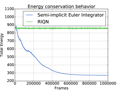
Figure 2: (a) Serial chain of $N$-bodies connected by revolute joints, (b) Energy conservation behavior over simulation frames

We first show that our linear-time variational integrator inherits the energy conservation property, which is one of the important features of variational integrators. We simulate a serial chain that consists of $N$-bodies connected by revolute joints (Fig. 2 (a)) with RIQN (variational integrator) and semi-implicit Euler method, which is an easy-to-implement standard method. In this experiment, we use a 10-body serial chain with no joint actuation nor external forces except for the gravity. The total energy (kinetic energy + potential energy) of this passive system should remain constant.

Fig. 2 (b) shows the energy evolution of the serial chain over simulation frames for both integration methods. RIQN does not artificially dissipate the energy while the Euler method does.

4.3 Performance Comparisons

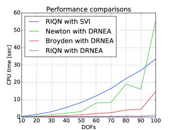
(a) Performance comparisons

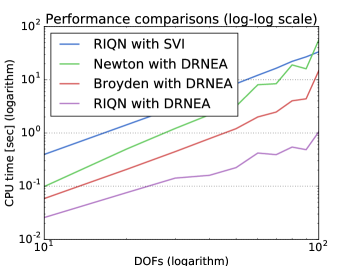
(b) Performance comparisons (logarithm)

Figure 3: Absolute computation time versus DOFs for the various root-finding methods.

The major factors that affect on the computational time of variational integrator are (1) evaluation of DEL equation and (2) the evaluation of Jacobian inverse. We consider various of the root-finding algorithm that are combination of methods for (1) and (2).

For (1), we compare our DRNEA to the scalable variational integrator (SVI) [6]. For (2), we compare the proposed RIQN to Newton’s method and Broyden method (quasi-Newton method) [19].

Newton’s method requires the (exact) Jacobian of the DEL equation. When combining with DRNEA, for a fair comparison we also derive a recursive algorithm to evaluate the derivatives of the DEL equation with respect to $\mathbf{q}^{k+1}$. Please see the Appendix for the algorithm.

For all the root-finding methods, we measure computation time of serial chain forward dynamics simulations for 10k frames. To reveal the scalability of the methods, we vary the number of bodies of the serial chain (Fig. 3). RIQN method with DRNEA shows the best performance. We also noticed that, for the same method for (2), DRNEA shows better performance than SVI. Further analyses show that the impulse-based Jacobian approximation contributes more than our linear-time DEL algorithm for the higher DOFs systems.

4.4 Convergence

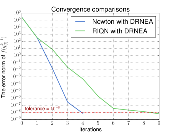
(a)

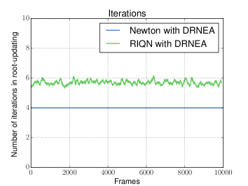
(b)

Figure 4: (a) Convergence rate comparison for Newton’s method and RIQN (b) Iteration numbers over simulation frames. Newton’s method: mean = 4, $\sigma=0.0$. RIQN: mean = 5.69, $\sigma=1.16$

We consider the convergent rate of RIQN comparing to Newton’s method. We inspect the convergence of error $f(\mathbf{q}_{(l)}^{k+1})=\mathbf{e}$ during the iterations in solving the DEL equation for one simulation time step. For quantitatively visible convergence, we use the zero configurations as the initial guess $\mathbf{q}_{0}^{k+1}=0$ instead of the proposed initial guesses in Section 3.3.

Fig. 4(a) shows that under the tolerance RIQN converges more slowly than Newton’s method. This observation is expected because Newton’s method has a quadratic convergence rate which is in theory faster than that of Quasi-Newton methods. However, in Section 4.3, we observed that the absolute computation time of the proposed method (DRNEA+RIQN) showed the best performance.

Fig. 4(b) shows the average iteration numbers per each simulation step in the root-finding process. As expected, Newton’s method requires less iteration numbers than RIQN.

5 Conclusion

We introduced a novel linear-time variational integrator for simulating multibody dynamic systems. At each simulation time step, the integrator solves a root-finding problem for the DEL equation using our quasi-Newton algorithm, RIQN, which consists of two primary contributions:

• DRNEA: Based on the variational integrator on Lie group and inspired by RNEA, we derived an $O(n)$ recursive algorithm that evaluates DEL equations of tree-structured multibody systems. Unlike the previous work, which formulates and solves the DEL equation for the entire system, in our approach the DEL equation for each body is solved recursively.

• Root updating: By leveraging existing forward dynamic algorithm for multibody systems, we introduced an $O(n)$ impulse-based dynamic algorithm to estimate the configuration at next time step.

We evaluated our linear-time variational integrator on a n-DOF open chain system and compared the results with existing state-of-art algorithms. The results show that, for the same computation method of root updating, the performance of our recursive evaluation of the DEL equation (linear-time DEL algorithm) is 15 times faster for a system with 10 degrees of freedom (DOFs) and 32 times faster for 100 DOFs. For the same evaluation method of the DEL equation (i.e., linear-time DEL algorithm), our results show that the performance of our new quasi-Newton method is 3.8 times faster for a system with 10 DOFs, and 53 times faster for 100 DOFs. Further analysis shows that for higher DOF systems, the impulse-based Jacobian approximation becomes increasingly more effective compared to our linear-time DEL algorithm.

One of the future directions is to apply the linear-time variational integrator on constrained dynamic systems. This paper demonstrates the performance gain on multibody systems with joint constraints, but does not address other types of constrains, such as contacts or closed-loop chains. The standard way to handle constraints in a dynamic system is to solve the DEL equations and constraints simultaneously using Lagrangian multipliers [1, 2]. To preserve the performance gain achieved by RIQN, one possible extension to constrained systems is to solve constraint force using the similar idea of impulse-based forward dynamics [8, 20].

Our current implementation of RIQN can be improved by using variable time step size. Although the variational integrator allows for larger time step size than other numerical integrators for the same accuracy, the variable time step size can still be exploited to achieve further stability and time performance. However, naively changing the time step size can have negative impact on the qualitative behavior of a simulation [15, 21]. Previous work has shown that additional constraints are needed when using the scheme of variable time step size. Integrating this line of work to our linear-time variational integrator can be a fruitful future research direction.

Appendix: Derivative of DRNEA

Algorithm 4 Derivative of DRNEA for computing $\frac{\partial{f(\mathbf{q}^{k+1})}}{\partial{\mathbf{q}^{k+1}}}\in\mathbb{R}^{n\times n}$

1:for $j=1\to n$ do

2:     for $i=1\to n$ do

3:         $\frac{\partial{T_{\lambda(i),i}^{k+1}}}{\partial{q_{j}^{k+1}}}=T_{\lambda(i),i}^{k+1}[S_{i}]\delta_{ij}$ $\triangleright$ $\delta_{ij}=\begin{cases}1,&\text{if }i=j\\ 0,&\text{otherwise}\end{cases}$

4:         $\frac{\partial{\Delta T_{i}^{k}}}{\partial{q_{j}^{k+1}}}=\left.T_{\lambda(i),i}^{k}\right.^{-1}\frac{\partial{\Delta T_{\lambda(i)}^{k}}}{\partial{q_{j}^{k+1}}}T_{\lambda(i),i}^{k+1}+\Delta T_{i}^{k}[S_{i}]\delta_{ij}$

5:         $\left[\frac{\partial{V_{i}^{k}}}{\partial{q_{j}^{k+1}}}\right]=\frac{1}{\Delta t}\text{{d}log}_{\Delta tV_{i}^{k}}\left(\frac{\partial{\Delta T_{i}^{k}}}{\partial{q_{j}^{k+1}}}\exp\left(-\Delta t[V_{i}^{k}]\right)\right)$

6:     end for

7:     for $i=n\to 1$ do

8:         $\frac{\partial{\mu_{i}^{k}}}{\partial{q_{j}^{k+1}}}=\frac{\partial{}}{\partial{q_{j}^{k+1}}}\left[\text{{d}log}_{\Delta tV_{i}^{k}}\right]^{T}G_{i}V_{i}^{k}+\left[\text{{d}log}_{\Delta tV_{i}^{k}}\right]^{T}G_{i}\frac{\partial{V_{i}^{k}}}{\partial{q_{j}^{k+1}}}$

9:         $\frac{\partial{F_{i}^{k}}}{\partial{q_{j}^{k+1}}}=\frac{\partial{\mu_{i}^{k}}}{\partial{q_{j}^{k+1}}}+\sum_{c\in\sigma(i)}\left[\text{Ad}_{\left(T_{i,c}^{k}\right)^{-1}}\right]^{T}\frac{\partial{F_{c}^{k}}}{\partial{q_{j}^{k+1}}}-\frac{\partial{F_{i}^{\text{ext},k}}}{\partial{q_{j}^{k+1}}}$

10:         $\frac{\partial{f(q^{k+1})}}{\partial{q_{j}^{k+1}}}=S_{i}^{T}\frac{\partial{F_{i}^{k}}}{\partial{q_{j}^{k+1}}}-\frac{\partial{Q_{i}^{k}}}{\partial{q_{j}^{k+1}}}$ $\triangleright$ $j$-th column of $\frac{\partial{f(\mathbf{q}^{k+1})}}{\partial{\mathbf{q}^{k+1}}}$

11:     end for

12:end for

References

- [1] Marsden, J.E., West, M.: Discrete mechanics and variational integrators. Acta Numerica 2001 10 (2001) 357–514
- [2] West, M.: Variational integrators. PhD thesis, California Institute of Technology (2004)
- [3] Betsch, P., Leyendecker, S.: The discrete null space method for the energy consistent integration of constrained mechanical systems. part ii: Multibody dynamics. International journal for numerical methods in engineering 67(4) (2006) 499–552
- [4] Leyendecker, S., Marsden, J.E., Ortiz, M.: Variational integrators for constrained dynamical systems. ZAMM-Journal of Applied Mathematics and Mechanics/Zeitschrift für Angewandte Mathematik und Mechanik 88(9) (2008) 677–708
- [5] Leyendecker, S., Ober-Blöbaum, S., Marsden, J.E., Ortiz, M.: Discrete mechanics and optimal control for constrained systems. Optimal Control Applications and Methods 31(6) (2010) 505–528
- [6] Johnson, E.R., Murphey, T.D.: Scalable variational integrators for constrained mechanical systems in generalized coordinates. Robotics, IEEE Transactions on 25(6) (2009) 1249–1261
- [7] Luh, J.Y., Walker, M.W., Paul, R.P.: On-line computational scheme for mechanical manipulators. Journal of Dynamic Systems, Measurement, and Control 102(2) (1980) 69–76
- [8] Featherstone, R.: Rigid body dynamics algorithms. Springer (2014)
- [9] Park, F.C., Bobrow, J.E., Ploen, S.R.: A lie group formulation of robot dynamics. The International Journal of Robotics Research 14(6) (1995) 609–618
- [10] Lee, T.: Computational geometric mechanics and control of rigid bodies. ProQuest (2008)
- [11] Kobilarov, M.B., Marsden, J.E.: Discrete geometric optimal control on lie groups. Robotics, IEEE Transactions on 27(4) (2011) 641–655
- [12] Kobilarov, M., Crane, K., Desbrun, M.: Lie group integrators for animation and control of vehicles. ACM Transactions on Graphics (TOG) 28(2) (2009) 16
- [13] Murray, R.M., Li, Z., Sastry, S.S.: A mathematical introduction to robotic manipulation. CRC press (1994)
- [14] Bou-Rabee, N., Marsden, J.E.: Hamilton–pontryagin integrators on lie groups part i: Introduction and structure-preserving properties. Foundations of Computational Mathematics 9(2) (2009) 197–219
- [15] Hairer, E., Lubich, C., Wanner, G.: Geometric numerical integration: structure-preserving algorithms for ordinary differential equations. Volume 31. Springer Science & Business Media (2006)
- [16] Fan, T., Murphey, T.: Structured linearization of discrete mechanical systems on lie groups: A synthesis of analysis and control. In: 2015 54th IEEE Conference on Decision and Control (CDC), IEEE (2015) 1092–1099
- [17] Liu, C.K., Stillman, M., Lee, J., Grey, M.X.: DART - Dynamic Animation and Robotics Toolkit. (2011 (accessed October 30, 2016)) http://dartsim.github.io.
- [18] Liu, C.K., Jain, S.: A short tutorial on multibody dynamics. Technical Report GIT-GVU-15-01-1, Georgia Institute of Technology, School of Interactive Computing (08 2012)
- [19] Broyden, C.G.: A class of methods for solving nonlinear simultaneous equations. Mathematics of computation 19(92) (1965) 577–593
- [20] Mirtich, B., Canny, J.: Impulse-based simulation of rigid bodies. In: Proceedings of the 1995 symposium on Interactive 3D graphics, ACM (1995) 181–ff
- [21] Kharevych, L.: Geometric interpretation of physical systems for improved elasticity simulations. PhD thesis, Citeseer (2009)