Two-color above threshold ionization of atoms and ions in XUV Bessel beams and combined with intense laser light

Abstract

The two-color above-threshold ionization (ATI) of atoms and ions is investigated for a vortex Bessel beam in the presence of a strong near-infrared (NIR) light field. While the photoionization is caused by the photons from the weak but extreme ultra-violet (XUV) vortex Bessel beam, the energy and angular distribution of the photoelectrons and their sideband structure are affected by the plane-wave NIR field. We here explore the energy spectra and angular emission of the photoelectrons in such two-color fields as a function of the size and location of the target atoms with regard to the beam axis. In addition, analogue to the circular dichroism in typical two-color ATI experiments with circularly polarized light, we define and discuss seven different dichroism signals for such vortex Bessel beams that arise from the various combinations of the orbital and spin angular momenta of the two light fields. For localized targets, it is found that these dichroism signals strongly depend on the size and position of the atoms relative to the beam. For macroscopically extended targets, in contrast, three of these dichroism signals tend to zero, while the other four just coincide with the standard circular dichroism, similar as for Bessel beams with small opening angle. Detailed computations of the dichroism are performed and discussed for the $4s$ valence-shell photoionization of Ca⁺ ions.

I Introduction

Studies on non-perturbative multiphoton processes in intense laser pulses have rapidly advanced during recent years and helped to explore the inner-atomic motion of electrons at femto- and attosecond timescales Corkum and Krausz (2007); Krausz and Ivanov (2009); Pazourek et al. (2015). For example, such multiphoton ionization and inner-shell processes have not only been observed for noble gases Gilbertson et al. (2010); Feist et al. (2009) but also for molecules Haessler et al. (2010), surfaces and elsewhere Cavalieri et al. (2007); Krüger et al. (2012). Today, these studies enable one to generate quite routinely attosecond pulses by high-order harmonic generation Sansone et al. (2006); Popmintchev et al. (2012); Calegari et al. (2016), or to control the above-threshold ionization (ATI) Milošević et al. (2006); Wittmann et al. (2009).

In typical ATI experiments, an electron is released from an atom or molecule by absorbing one or several photons from a near-infrared (NIR) laser field more than required energetically in order to overcome the ionization threshold. The ATI energy spectra of the photoelectrons therefore exhibit a series of peaks, just separated by the NIR photon energy, while the relative strength of these peaks may depend significantly on the intensity and temporal structure of the incident laser pulses. These ATI spectra are thus quite in contrast to the photoelectron spectra as obtained by just weak high-frequency (XUV) radiation, where the absorption of a single photon is sufficient to eject a bound electron and where the single photoline (for each possible final state of the photoion) is usually well described by perturbation theory. In two-color ATI, such a XUV field is often combined with intense NIR laser pulses in order to investigate the ionization of sub-valence electrons: While, under these circumstances, the NIR field alone is not sufficient to ionize the atoms or molecules efficiently, it is intense enough to stimulate the absorption or emission of one or several additional NIR photons by the outgoing electron. This non-perturbative interaction of the electrons with both, the XUV and NIR fields then leads to the well-known ’sidebands’ that typically occur as satellites to the normal photolines Ehlotzky (2001); Radcliffe et al. (2012). Such sidebands were first observed in the two-color ATI of noble gases as well as in laser-assisted Auger processes Muller et al. (1986); Schins et al. (1994); Glover et al. (1996); Meyer et al. (2006, 2008, 2010). More recently, these sidebands have been applied in pump-probe photoelectron spectroscopy Helml et al. (2014) or in imaging the molecular orbitals of $\rm H_{2}O$, $\rm O_{2}$ and $\rm N_{2}$ Leitner et al. (2015).

Apart from the temporal structure of the XUV and NIR pulses, the intensity of the sidebands depends of course also on the relative orientation and linear polarization of these fields O’Keeffe et al. (2004); Guyétand et al. (2005). This orientation dependence has been explored especially by Meyer and coworkers Meyer et al. (2008) for the angular distribution of the sidebands in the photoionization of helium. Later, it was shown theoretically Kazansky et al. (2012) that the two-color ATI sideband spectra are rather sensitive also with regard to the circular polarization of both, the XUV and NIR light, and an asymmetry in the photoelectron spectra was found, if the circular polarization of one of the field is changed from same to the opposite direction, a phenomenon that is termed today as circular dichroism in two-color ATI. This circular dichroism, that is associated with some flip of the spin-angular momentum (SAM) of the incident light field, has recently been utilized, e.g., for measuring the polarization state of an ultra-violet free electron laser Kazansky et al. (2011, 2012); Mazza et al. (2014). For molecules, in addition, the question has been raised how two-color ATI spectra are affected by the molecular symmetry and the polarization of the incident radiation Guyétand et al. (2008); Lux et al. (2012).

In this work, we investigate the two-color ATI process if the usual plane-wave XUV field is replaced by a vortex (Bessel) beam, also known as ’twisted light’, that carries not only SAM but also orbital angular momentum (OAM). Indeed, the study of such OAM light has attracted much recent interest for the manipulation of microparticles Molina-Terriza et al. (2007), for investigating fundamental interactions Stock et al. (2015); Quinteiro et al. (2015); Surzhykov et al. (2015); Schmiegelow et al. (2016); Radwell et al. (2015), and for multiplexing in telecommunication Bozinovic et al. (2013); Krenn et al. (2014), to name a few. In particular, we here explore the energy spectra and angular emission of photoelectrons ejected by a vortex Bessel beam in the presence of strong NIR light, and how these photoelectron spectra depend on the size and location of the target (atoms) with regard to the axis of the vortex beam. We assume an XUV Bessel beam that is energetic enough to photoionize the atom, while the plane-wave NIR field affects the sideband structure as well as the energy and angular distribution of the photoelectrons. Analogously to the circular dichroism from above, we define and discuss moreover seven possible dichroism signals which arise from different combinations of the orbital and spin angular momenta of the two light fields involved. For localized targets, we find that these dichroism signals sensitively depend on the size and position of the atoms relative to the beam axis. For macroscopically extended targets, in contrast, three of these signals tend to zero, while the other four just approach the (standard) circular dichroism. To discuss these finding, detailed computations of the dichroisms are performed and discussed for the $4s$ valence-shell photoionization of Ca⁺ ions.

In the next section, we shall first evaluate the transition amplitude and photoionization probability for the two-color ATI within the strong-field approximation (SFA), if a vortex Bessel beam interacts with an atom in the presence of a strong, plane-wave NIR field. Note that atomic units are used throughout the paper. Details about the twisted XUV Bessel beam are given in Subsection II.2, while the choice of targets is explained in Subsection II.4. The possible dichroism signals for such a two-color field are defined in Section II.5 . Emphasize is placed here especially on the influence of a localized versus macroscopically extended target in exploring the sensitivity of the dichroism with regard to the target size. Detailed calculations of the photoelectron spectra and the various dichroism signals are presented and discussed later in Section III. Finally, conclusions are given in Section IV.

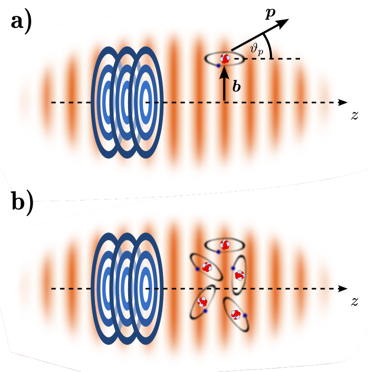
Figure 1: Scheme for the two-color ATI of an atom by an XUV vortex beam (blue) and in the presence of a strong NIR field (orange). The atoms are assumed to be either a) localized with regard to the common beam axis or b) equally distributed over the cross section of the XUV Bessel beam.

II Theoretical Background

II.1 Two-color ATI in Strong-Field Approximation

We here explore the two-color ATI of atoms (and ions) if they interact with a weak XUV vortex beam and an intense plane-wave NIR field. In particular, we assume an (almost) monochromatic XUV vortex beam, as for instance generated by free-electron lasers (FEL), and which is energetic enough to ionize the target atom. Although quite strong, moreover, we suppose some NIR laser pulse with many optical cycles so that it can be described as a monochromatic plane-wave. Together, these two assumptions ensure that the ’sideband regime’ holds Radcliffe et al. (2012), in which photoelectrons are expected not only at the given photoline but also at energies that differ by one or several energy quanta of the the NIR field. Moreover, both fields are supposed to propagate along a common beam axis that is taken also as the quantization axis ($z$-axis). Finally, the atomic target is either a microscopic target of trapped atoms or ions, localized at some position $\boldsymbol{b}$ in the $xy$-plane perpendicular to the beam axis, cf. Ref. Schmiegelow et al. (2016) and Fig. 1a, or as macroscopic and uniformly distributed target over the cross section of the twisted XUV beam (Fig. 1b).

After their interaction with the two-color field, the photoelectrons leave the interaction region with the asymptotic (canonical) momentum $\boldsymbol{p}$ as measured at the detectors. Below, we shall analyze the angular and momentum distribution of these electrons as a function of the polar angle $\vartheta_{p}$ of the momentum, i.e. with regard to the common beams axis, as well as for different azimuth angles $\varphi_{p}$ [as defined by the impact vector $\boldsymbol{b}\,=\,(b,\varphi_{p}=0,z=0)$ of the target atom]. In particular, we aim to understand how the photoelectron distributions are affected by the OAM of the XUV beam and by relative changes in either the SAM and/or OAM of the two-color fields.

Within the SFA, the transition amplitude $\mathcal{T}$ for the two-color ATI of a single active electron, being initially in the bound state $|\phi_{0}\rangle$, reads as

$$\mathcal{T}(\boldsymbol{p}) =-i\int_{-\infty}^{\infty}\!{\mathrm{d}}t\,\left\langle\Psi^{(V)}_{\boldsymbol{q}(t)}\left|\,\boldsymbol{\hat{p}}\cdot\boldsymbol{A}_{X}(\boldsymbol{r})\,\vphantom{\Psi^{(V)}_{\boldsymbol{q}(t)}}\right|\phi_{0}\right\rangle\;e^{i\,(E_{B}-\omega_{X})t}\,,$$ (1)

where $E_{B}$ is the binding energy of the active electron and $\boldsymbol{A}_{X}(\boldsymbol{r})$ the vector potential of the XUV Bessel beam with frequency $\omega_{X}$. We shall describe the details of this vector potential in the next subsection. In the SFA, moreover, the final (continuum) state of the electron is typically described by a Volkov state $\left\langle\Psi^{(V)}_{\boldsymbol{q}(t)}\right|=\left\langle\boldsymbol{q}(t)\right|\,e^{-iS_{V}(t)}$ (in length gauge), which neglects the effect of the parent ion upon the motion of the liberated electron, and where $\left\langle\boldsymbol{q}(t)\right|$ describes the plane-wave electron wave function with the kinetic momentum $\boldsymbol{q}(t)=\boldsymbol{p}-\boldsymbol{A}_{L}(t)$. In the presence of an external NIR field $\boldsymbol{A}_{L}(t)$, this kinetic momentum is different from the conserved canonical momentum $\boldsymbol{p}$ which is measured at the detector, eventually. Finally, the phase of the Volkov wavefunction is given by Volkov (1935)

$$S_{V}(t) =\int_{t}^{\infty}\!{\mathrm{d}}t^{\prime}\,\frac{\boldsymbol{q}(t)^{2}}{2}=\frac{1}{2}\int_{t}^{\infty}\!{\mathrm{d}}t^{\prime}\,\left[\boldsymbol{p}-\boldsymbol{A}_{L}(t^{\prime})\right]^{2}\,.$$ (2)

While we have employed the length gauge for the strong assisting NIR laser field $\boldsymbol{A}_{L}$, we still use the interaction operator with the high-frequency XUV vortex field $\boldsymbol{A}_{X}$ in the velocity gauge form because of the complex spatial structure of $\boldsymbol{A}_{X}(\boldsymbol{r})$.

II.2 Characterization of twisted Bessel beams

So-called twisted or vortex (light) beams are known to carry, in addition their possible polarization or SAM, also an orbital angular momentum (OAM) owing to their helical phase fronts. Typically, twisted beams show a very characteristic annular intensity distribution with zero intensity on the beam axis. This zero intensity line is called the vortex line of the field and it embodies a phase singularity. In the XUV frequency region, twisted light beams have been generated recently by means of undulators Hemsing et al. (2013); Bahrdt et al. (2013) or by using high-harmonic generation Zürch et al. (2012); Gariepy et al. (2014); Hernández-García et al. (2013). Experimentally, such twisted beams can be prepared in different modes with regard to the (components of the) angular momenta that are conserved for some given beam. In the further analysis, we shall assume Bessel beams that are obtained as non-paraxial solutions of the vector Helmholtz equation, and which are classified here by the wave vector components $k_{z}$ and $\varkappa$ [with $\varkappa=|\boldsymbol{k}_{\perp}|$ and $\boldsymbol{k}\>\equiv\>(\boldsymbol{k}_{\perp},k_{z})^{T}\>=\>(\varkappa,\varphi_{k},k_{z})$], the topological charge $m$ as well as the helicity $\Lambda_{X}$.

Here, we shall restrict ourselves to the representation of the vector potential of these Bessel beams in terms of plane waves and how we can distinguish between their spin-angular (polarization) and orbital angular momenta. Following Refs. Jentschura and Serbo (2011); Ivanov and Serbo (2011); Matula et al. (2013), we can write the vector potential

$$\boldsymbol{A}_{X}(\boldsymbol{r}) =\int\!\frac{\mathrm{d}^{2}\boldsymbol{k}_{\perp}}{(2\pi)^{2}}\>a_{\varkappa m}(\boldsymbol{k}_{\perp})\>e^{i\boldsymbol{k}\cdot\boldsymbol{r}}\,\boldsymbol{\varepsilon}_{\boldsymbol{k}\Lambda_{X}}\,,$$ (3)

as a superposition of plane waves with wave vectors $\boldsymbol{k}=(\boldsymbol{k}_{\perp},k_{z})^{T}$ and the Fourier coefficients

$$a_{\varkappa m}(\boldsymbol{k}_{\perp}) =\sqrt{\frac{2\pi}{\varkappa}}\>(-i)^{m}e^{im\varphi_{k}}\>\delta(k_{\perp}-\varkappa)\,,$$ (4)

and where $\vartheta_{k}=\arctan\varkappa/k_{z}$ is the so-called cone opening angle. Like in the atomic case, the (quantum) number $m$ determines the projection of the OAM or the so-called topological charge and $\boldsymbol{\varepsilon}_{\boldsymbol{k}\Lambda_{X}}$ the polarization (vector) of the plane-wave components. Obviously, the polarization vector must depend explicitly not only on the helicity $\Lambda_{X}$ of the plane-wave components, but also on the angles $\vartheta_{k}$ and $\varphi_{k}$,

$$\boldsymbol{\varepsilon}_{\boldsymbol{k}\Lambda_{X}} =\frac{e^{i\Lambda_{X}\varphi_{k}}}{\sqrt{2}}\left(\begin{matrix}\cos\vartheta_{k}\cos\varphi_{k}-i\Lambda_{X}\sin\varphi_{k}\\ \cos\vartheta_{k}\sin\varphi_{k}+i\Lambda_{X}\cos\varphi_{k}\\ -\sin\vartheta_{k}\end{matrix}\right)\,,$$ (5)

due to the transversality condition $\boldsymbol{k}\cdot\boldsymbol{\varepsilon}_{\boldsymbol{k}\Lambda_{X}}\>=\>0$. Indeed, this definition of the polarization vector $\boldsymbol{\varepsilon}_{\boldsymbol{k}\Lambda_{X}}$ ensures that, in the limit of small opening angles $\vartheta_{k}\to 0$, we obtain the usual polarization vectors for circularly polarized plane waves

$$\boldsymbol{\varepsilon}_{\boldsymbol{k}\Lambda_{X}}\stackrel{{\scriptstyle\vartheta_{k}\to 0}}{{\to}}\frac{1}{\sqrt{2}}\>(1,i\Lambda_{X},0)^{T}\,.$$ (6)

It can be shown Matula et al. (2013) that the polarization vector $\boldsymbol{\varepsilon}_{\boldsymbol{k}\Lambda_{X}}$ from Eq. (5) is an eigenvector also of the $z$-component $\hat{J}_{z}\,=\,\hat{L}_{z}+\hat{S}_{z}$ of the total angular momentum operator with eigenvalues $m_{J}=\Lambda_{X}$: $\>\hat{J}_{z}\>\boldsymbol{\varepsilon}_{\boldsymbol{k}\Lambda_{X}}\,=\,\Lambda_{X}\>\boldsymbol{\varepsilon}_{\boldsymbol{k}\Lambda_{X}}$. With this definition of $\boldsymbol{\varepsilon}_{\boldsymbol{k}\Lambda_{X}}$, the Bessel beam (3) is constructed as an eigenfunction of the total angular momentum projection $\hat{J}_{z}$ with eigenvalue $m_{J}=m+\Lambda_{X}$ :

$$\hat{J}_{z}\boldsymbol{A}_{X}(\boldsymbol{r})=(m+\Lambda_{X})\boldsymbol{A}_{X}(\boldsymbol{r})\,.$$

For the sake of completeness, let us write here the vector potential of the XUV Bessel beam explicitly in cylindrical co-ordinates

$$\boldsymbol{A}_{X}(\boldsymbol{r})=\sum_{m_{s}=-1,0,1}\boldsymbol{\eta}_{m_{s}}\>\sqrt{\frac{\varkappa}{2\pi}}\>c_{m_{s}}\>e^{ik_{z}z}\>i^{\Lambda_{X}-m_{s}}\\[2.84544pt] \times\>e^{i(m+\Lambda_{X}-m_{s})\varphi}\>J_{m+\Lambda_{X}-m_{s}}(\varkappa r_{\perp})\,.$$ (7)

In this expression, $\boldsymbol{\eta}_{0}=(0,0,1)$ and $\boldsymbol{\eta}_{\pm 1}=(1,\pm i,0)/\sqrt{2}$ denote the (spherical) unit vectors, and the coefficients are $c_{0}=-(\sin\vartheta_{k})/\sqrt{2}$ and $c_{\pm 1}=(\cos\vartheta_{k}\pm\Lambda_{X})/2$, respectively. As seen from Eq. (7), a Bessel beam consist of three terms with topological charges $m+\Lambda_{X}$ and $m+\Lambda_{X}\pm 1$. The relative weight of these terms depend on the opening angle $\vartheta_{k}$, and only the one with the topological charge $m$ remains non-zero for paraxial beams, i.e. if $\vartheta_{k}\ll 1$ .

II.3 Transition amplitude for a well-localized atom in a XUV Bessel beam

We can use the vector potential of the XUV Bessel beam, Eq. (3), to evaluate the transition amplitude (1) for the two-color ATI of atoms and ions and for the emission of photoelectrons with well-defined asymptotic momentum $\boldsymbol{p}$. To do so, we also need to specify the position of the atom with regard to the beam axis, i.e. in terms of an impact parameter vector $\boldsymbol{b}\>\equiv\>(b,\varphi_{b}=0,b_{z}=0)$. If $\boldsymbol{r}$ denotes the electronic coordinate with respect to the atomic nucleus, that is the center of the atomic potential, we have to replace $\boldsymbol{r}\,\to\,\boldsymbol{b}+\boldsymbol{r}$ in the electron-photon interaction operator. We therefore see that, for vortex beams, the transition amplitude generally depends on the location of the atom within the beam, as indicated by the subscript $\boldsymbol{b}$ in the notation of the transition amplitude:

$$\mathcal{T}_{\boldsymbol{b}}(\boldsymbol{p}) =\int\!\frac{\mathrm{d}^{2}\boldsymbol{k}_{\perp}}{(2\pi)^{2}}\>a_{\varkappa m}(\boldsymbol{k}_{\perp})\>e^{i\boldsymbol{k}\cdot\boldsymbol{b}}\>\mathcal{T}^{\rm pw}({\boldsymbol{p},\boldsymbol{k}})\,.$$ (8)

It is readily expressed as a superposition of typical SFA plane-wave amplitudes

$$\mathcal{T}^{\rm pw}(\boldsymbol{p},\boldsymbol{k})=-i\int\!{\mathrm{d}}t\,\boldsymbol{q}(t)\cdot\boldsymbol{\varepsilon}_{\boldsymbol{k}\Lambda_{X}}\,e^{i(E_{B}-\omega_{X})t-iS_{V}(t)}\\ \times\,\left\langle\boldsymbol{q}(t)\left|\>e^{i\,\boldsymbol{k}\cdot\boldsymbol{r}}\>\right|\phi_{0}\right\rangle\,,$$ (9)

just weighted by the Fourier coefficients $a_{\varkappa m}(\boldsymbol{k}_{\perp})$ of the Bessel beam and the given phase factor $e^{i\boldsymbol{b}\cdot\boldsymbol{k}}$. An analogue superposition of plane-wave amplitudes was found also for the single-photon ionization by light from a vortex beam Surzhykov et al. (2015), and this remains true when adding an assisting laser field, at least within the SFA. Let us mention finally that all the time-dependence resides in the plane-wave amplitudes $\mathcal{T}^{\rm pw}(\boldsymbol{p},\boldsymbol{k})$.

II.3.1 Time-dependence of the Volkov phase: Sideband structure

To obtain and describe the (well-known) sideband structures in the energy spectrum of the emitted photoelectrons in the two-color ATI, we next need to specify the vector potential of the strong NIR laser pulse that enters the plane-wave amplitude $\mathcal{T}^{\rm pw}(\boldsymbol{p},\boldsymbol{k})$. For the strong laser pulse, we here apply the vector potential

$$\boldsymbol{A}_{L}(t) =A_{L}\left(\begin{matrix}\cos\omega_{L}t\\[2.84544pt] \Lambda_{L}\sin\omega_{L}t\\[2.84544pt] 0\end{matrix}\right)\,,$$ (10)

of a plane wave with laser frequency $\omega_{L}$, helicity $\Lambda_{L}$ and field amplitude $A_{L}$. In the plane-wave amplitude of Eq. (9), moreover, we can cast the Volkov phase factor into the form

$$e^{-iS_{V}(t)}=e^{i(\frac{p^{2}}{2}+U_{p})t}\sum_{\ell={-\infty}}^{\infty}J_{\ell}(\alpha_{L})e^{-i\ell(\omega_{L}t-\Lambda_{L}\varphi_{p})}$$ (11)

by applying the Jacobi-Anger expansion Watson (1922), and where $\alpha_{L}=(A_{L}\,p\sin\vartheta_{p})/\omega_{L}$ just refers to the amplitude of the classical oscillation of an electron in the laser field, while $U_{p}\,=\,A_{L}^{2}/2$ is the ponderomotive potential.

With this reformulation of the Volkov phase factor in Eq. (11), the (strong-field) transition amplitude $\mathcal{T}^{\rm pw}(\boldsymbol{p},\boldsymbol{k})$ therefore becomes

$$\mathcal{T}^{\rm pw}(\boldsymbol{p},\boldsymbol{k}) =-i\sum_{\ell}J_{\ell}(\alpha_{L})\>e^{i\ell\Lambda_{L}\varphi_{p}}\,\int\!{\mathrm{d}}t\>e^{i(\frac{p^{2}}{2}+U_{p}+E_{B}-\omega_{X}-\ell\omega_{L})t}\>\boldsymbol{q}(t)\cdot\boldsymbol{\varepsilon}_{\boldsymbol{k}\Lambda_{X}}\>\left\langle\boldsymbol{q}(t)\left|\,e^{i\boldsymbol{k}\cdot\boldsymbol{r}}\,\right|\phi_{0}\right\rangle\,.$$ (12)

To further simplify this amplitude we next have to analyze the scalar product between the kinetic momentum $\boldsymbol{q}(t)$ of the electron and the polarization vector of the twisted light $\boldsymbol{\varepsilon}_{\boldsymbol{k}\Lambda_{X}}$ in the following subsection.

Before we shall continue, let us note, that the summations in Eqs. (11) and (12) formally runs from $\ell=-\infty\ldots\infty$. In practice, however, just a finite number of sidebands, $\ell_{\mathrm{min}}\leq\ell\leq\ell_{\mathrm{max}}$, can be resolved experimentally, while the magnitude of these sidebands decays exponentially beyond these cut-off values. These cut-off values can be determined by either a saddle point analysis of the Volkov phase Lewenstein et al. (1994); Zhang et al. (2013); Seipt et al. (2015, 2016) or by just making use of the properties of the Bessel functions Watson (1922). From the prior analysis, we have found these cut-off values as

$$\ell_{\mathrm{max/min}}=\frac{A_{L}^{2}\sin^{2}\vartheta_{p}}{\omega_{L}}\pm\sqrt{\frac{A_{L}^{4}\sin^{4}\vartheta_{p}}{\omega_{L}^{2}}+2\frac{A_{L}^{2}\sin^{2}\vartheta_{p}}{\omega_{L}}\>(\omega_{X}-E_{B}-U_{p})}\,,$$ (13)

and where the upper/lower sign refer to the max/min values.

II.3.2 Angular dependence of the photoelectron emission in the transition amplitude

The angular distribution of the photoelectrons emitted in the two-color ATI process is mainly determined by the scalar product $\boldsymbol{q}(t)\cdot\boldsymbol{\varepsilon}_{\boldsymbol{k}\Lambda_{X}}$ in the plane-wave amplitudes (12). This scalar product becomes maximum when the kinetic momentum of the photelectron $\boldsymbol{q}(t)\,=\,\boldsymbol{p}-\boldsymbol{A}_{L}(t)$ is, at the moment of the ionization, parallel to the polarization vector of the XUV field. We remember that this kinetic momentum $\boldsymbol{q}(t)$ differs from the conserved canonical momentum $\boldsymbol{p}$ as long as the electron is inside the laser pulse.

Plane Waves:

Here, let us first (re-)consider the scalar product $\boldsymbol{q}(t)\cdot\boldsymbol{\varepsilon}_{\boldsymbol{k}\Lambda_{X}}$ for the case of circularly polarized plane waves Kazansky et al. (2012). If the XUV pulse propagates for instance along the $z$-direction, $\boldsymbol{k}=k\boldsymbol{e}_{z}$, we can apply the plane-wave limit of the XUV polarization vector from Eq. (6) and readily obtain for the scalar product

$$\boldsymbol{q}(t)\cdot\boldsymbol{\varepsilon}_{\boldsymbol{k}\Lambda_{X}} =\frac{p}{\sqrt{2}}\sin\vartheta_{p}e^{i\Lambda_{X}\varphi_{p}}-\frac{A_{L}}{\sqrt{2}}e^{i\Lambda_{X}\Lambda_{L}\omega_{L}t}\,.$$ (14)

Moreover, if we combine this expression with Eq. (12), the plane-wave transition amplitude reads as

$$\mathcal{T}^{\rm pw}(\boldsymbol{p},\boldsymbol{k}=k\boldsymbol{e}_{z}) =-i\sum_{\ell}\mathcal{F}_{\ell}(\Lambda_{L},\Lambda_{X})\,e^{i(\ell\Lambda_{L}+\Lambda_{X})\varphi_{p}}\>\int\!{\mathrm{d}}t\,e^{i(\frac{p^{2}}{2}+U_{p}+E_{B}-\omega_{X}-\ell\omega_{L})t}\left\langle\boldsymbol{q}(t)\left|\,e^{i\boldsymbol{k}\cdot\boldsymbol{r}}\,\right|\phi_{0}\right\rangle\,,$$ (15)

where the sideband amplitudes

$$\mathcal{F}_{\ell}(\Lambda_{L},\Lambda_{X}) =\frac{1}{\sqrt{2}}\Big{(}J_{\ell}(\alpha_{L})p\sin\vartheta_{p}-A_{L}J_{\ell+\Lambda_{L}\Lambda_{X}}(\alpha_{L})\Big{)}\,$$ (16)

describe the strength and the angular distribution of the photoelectrons of the $\ell$-th sideband (ATI-peak). In order to arrive at Eqs. (15) and (16), we have shifted the summation variable $\ell$ in the second term of Eq. (16).

From the sideband amplitude (16), we immediately find: (i) Only the central photoline ($\ell=0$) occurs with the typical $\mathbb{P}(\vartheta_{p})\propto\sin^{2}\vartheta_{p}$ angular dependence if the laser field vanishes, i.e. for $A_{L}\to 0$ and $\alpha_{L}\to 0$. Moreover, (ii) the second term of $\mathcal{F}_{\ell}$ in Eq. (16) contains the product $\Lambda_{L}\,\Lambda_{X}$ of the spin angular momenta (helicities) of the XUV and the NIR laser fields in the order of the Bessel function $J$. Therefore, the angular distribution of the photoelectrons differ from each other if $\Lambda_{X}$ and $\Lambda_{L}$ have either equal or opposite signs. Indeed, it is the sign of $\Lambda_{L}\,\Lambda_{X}$ that leads to the circular dichroism in the two-color photoionization of atoms by plane-wave radiation Kazansky et al. (2012); Mazza et al. (2014).

XUV Bessel beams:

Of course, the same scalar product in the plane-wave amplitude (12) becomes much more complex for a vortex beam (3) since it now depends explicitly on the direction of the momentum vector $\boldsymbol{k}\>=\>\boldsymbol{k}(\vartheta_{k},\varphi_{k})$ of the plane-wave components, forming a cone in momentum space. Using expression (5), this product can be evaluated as [compare with Eq. (14)]

$$\boldsymbol{q}(t)\cdot\boldsymbol{\varepsilon}_{\boldsymbol{k}\Lambda_{X}}=\frac{p}{\sqrt{2}}\>\left[\sin\vartheta_{p}e^{i\Lambda_{X}\varphi_{p}}\>-\>2\sin\vartheta_{p}\sin^{2}\frac{\vartheta_{k}}{2}\cos(\varphi_{p}\>-\>\varphi_{k})e^{i\Lambda_{X}\varphi_{k}}\>-\>\cos\vartheta_{p}\sin\vartheta_{k}e^{i\Lambda_{X}\varphi_{k}}\right]\\[4.26773pt] -\frac{A_{L}}{\sqrt{2}}\>\left[e^{i\Lambda_{X}\Lambda_{L}\omega_{L}t}\>-\>\sin^{2}\frac{\vartheta_{k}}{2}\left(e^{i\omega_{L}t}\,e^{i(\Lambda_{X}-\Lambda_{L})\varphi_{k}}+e^{-i\omega_{L}t}\,e^{i(\Lambda_{X}+\Lambda_{L})\varphi_{k}}\right)\right]\,.$$ (17)

If we substitute this expression into Eq. (9), the transition amplitude for the two-color ATI of an atom at position $\boldsymbol{b}$ by a XUV Bessel beam can be written as the superposition (8) of the plane-wave transition amplitudes

$$\mathcal{T}^{\rm pw}(\boldsymbol{p},\boldsymbol{k}) =-i\sum_{\ell}\mathcal{F}_{\ell}(\vartheta_{k},\varphi_{k};\Lambda_{X},\Lambda_{L})\>e^{i(\ell\Lambda_{L}+\Lambda_{X})\varphi_{p}}\>\int\!{\mathrm{d}}t\>e^{i(\frac{p^{2}}{2}+U_{p}+E_{B}-\omega_{X}-\ell\omega_{L})t}\,\left\langle\boldsymbol{q}(t)\left|\>e^{i\boldsymbol{k}\cdot\boldsymbol{r}}\>\right|\phi_{0}\right\rangle\,,$$ (18)

and with the modified sideband amplitudes

$$\mathcal{F}_{\ell}(\vartheta_{k},\varphi_{k};\Lambda_{X},\Lambda_{L})=J_{\ell}(\alpha_{L})\frac{p}{\sqrt{2}}\left[\sin\vartheta_{p}\>-\>2\sin\vartheta_{p}\sin^{2}\frac{\vartheta_{k}}{2}\cos(\varphi_{k}\>-\>\varphi_{p})e^{i\Lambda_{X}(\varphi_{k}-\varphi_{p})}\>-\>\cos\vartheta_{p}\sin\vartheta_{k}e^{i\Lambda_{X}(\varphi_{k}-\varphi_{p})}\right]\\[4.26773pt] -\frac{A_{L}}{\sqrt{2}}\left[J_{\ell+\Lambda_{X}\Lambda_{L}}(\alpha_{L})\>-\>\sin^{2}\frac{\vartheta_{k}}{2}\left\{J_{\ell+1}(\alpha_{L})e^{i(\Lambda_{X}-\Lambda_{L})(\varphi_{k}-\varphi_{p})}\>+\>J_{\ell-1}(\alpha_{L})e^{i(\Lambda_{X}+\Lambda_{L})(\varphi_{k}-\varphi_{p})}\right\}\right]\,,$$ (19)

which now depends on the particular direction of the wave vector $\boldsymbol{k}$.

II.3.3 Analytical time integration of the two-color ATI transition amplitude

The plane-wave transition amplitude (18) still contains a time integration which cannot be performed in general. However, this time integral can be solved analytically if we assume a sufficiently weak assisting NIR laser field, $A_{L}\ll p$, so that the kinetic momentum $\boldsymbol{q}(t)$ of the photoelectron can be reasonably well approximated by the canonical momentum $\boldsymbol{p}$ in the atomic matrix. This then results also in time-independent atomic matrix elements Kazansky et al. (2010, 2012). In the dipole approximation, moreover, we can approximate these matrix elements by

$$\left\langle\boldsymbol{q}(t)\left|\,e^{i\boldsymbol{k}\cdot\boldsymbol{r}}\,\right|\phi_{0}\right\rangle\>\simeq\>\langle\boldsymbol{p}|\phi_{0}\rangle\,,$$ (20)

which is valid almost everywhere apart from the region close to the vortex line. For $\boldsymbol{b}\,=\,0$, in contrast, the integral over the transverse momentum $\boldsymbol{k}_{\perp}$ in (8) vanishes when the electric-dipole approximation is employed, and the leading contribution to the twisted-wave amplitude $\mathcal{T}_{\boldsymbol{b}\simeq 0}(\boldsymbol{p})$ will then arise from higher-order multipoles Surzhykov et al. (2015); Schmiegelow et al. (2016).

With these assumptions about the NIR field, we can perform the time integration in the plane-wave amplitude (18)

$$\int\!{\mathrm{d}}t\,e^{it(\frac{p^{2}}{2}+U_{p}+E_{B}-\omega_{X}-\ell\omega_{L})}\\ =2\pi\,\delta(p^{2}/2+U_{p}+E_{B}-\omega_{X}-\ell\omega_{L})\,.$$ (21)

Here, the delta function ensures the energy conservation in this two-color interaction process and shows that the kinetic energy of the photoelectrons becomes discrete for sufficiently weak fields. In each of these sidebands of the main photo line (that arise from the ionization by the XUV pulse), the modulus of the electron momenta is constant, $|\boldsymbol{p}|=p\to p_{\ell}=\sqrt{2(\omega_{X}+\ell\omega_{L}-E_{B}-U_{p})}$, while these electrons may still exhibit an (angular) distribution as function $\vartheta_{p}$ and $\varphi_{p}$. Using expression (21), the transition amplitude for two-color ATI of an atom at position $\boldsymbol{b}$ by a XUV Bessel beam now becomes

$$\mathcal{T}_{\boldsymbol{b}}(\boldsymbol{p}) =2\pi\sum_{\ell}\>\delta(p^{2}/2+U_{p}+E_{B}-\omega_{X}-\ell\omega_{L})\>\mathcal{T}^{(\ell)}\,,$$ (22)

and where

$$\mathcal{T}^{(\ell)} =\langle\boldsymbol{p}_{\ell}|\phi_{0}\rangle\>\int\!\frac{\mathrm{d}^{2}\boldsymbol{k}_{\perp}}{(2\pi)^{2}}\,e^{i\boldsymbol{k}\cdot\boldsymbol{b}}\,a_{\varkappa m}(\boldsymbol{k}_{\perp})\mathcal{F}_{\ell}(\vartheta_{k},\varphi_{k};\Lambda_{X},\Lambda_{L})$$ (23)

are often referred to as partial amplitudes. As seen from expression (23), the angular distribution of the photoelectrons is now determined by a convolution of the sideband amplitudes $\mathcal{F}_{\ell}$ with the Fourier coefficients of the vortex Bessel beam $a_{\varkappa m}(\boldsymbol{k}_{\perp})$ from Eq. (4) and a phase factor that just contains the impact vector $\boldsymbol{b}$. Indeed, the expressions (22) and (23) are one of our major results of this work, although they still describe the transition amplitude for a single atom at some (fixed) position $\boldsymbol{b}$ with regard to the beam axis.

II.4 Photoionization probability of localized and macroscopically extended targets

We can use the two-color ATI amplitude (22) to express the photoionization probability (per unit time) for an atom at position $\boldsymbol{b}$ within a vortex beam by

$$\mathbb{P}_{\boldsymbol{b}}(\boldsymbol{p}) =\frac{1}{T}\left|\mathcal{T}_{\boldsymbol{b}}(\boldsymbol{p})\right|^{2}$$

$$=2\pi\sum_{\ell}\delta(p^{2}/2+U_{p}+E_{B}-\omega_{X}-\ell\omega_{L})\mathbb{P}^{(\ell)}_{\boldsymbol{b}}(\boldsymbol{p})\,,$$ (24)

if $T$ denotes here the interaction time of the atom with the two-color field, and if we make use of the usual interpretation of the delta function $\delta(0)=T/2\pi$ in the second line. Expression (24) shows that the photoionization probability is a sum of partial probabilities

$$\mathbb{P}^{(\ell)}_{\boldsymbol{b}}(\boldsymbol{p})=\left|\mathcal{T}^{(\ell)}\right|^{2}$$ (25)

that describe the individual sidebands in the photoelectron spectrum. The partial probabilities (25) still refer, as before, to a single atom at impact vector $\boldsymbol{b}$ with regard to the beam axis. To further analyze and compare the photoelectron spectra and angular distribution with those obtained experimentally, we need to know (or assume) also the distribution of atoms in the overall cross section of the Bessel beam.

II.4.1 Macroscopically extended targets

If, for example, the twisted Bessel beam interacts with a homogeneous and (infinitely in the cross section of the beam) extended target of atoms, we have to average the partial photoionization probabilities $\mathbb{P}^{(\ell)}_{\boldsymbol{b}}(\boldsymbol{p})$ from Eq. (25) incoherently over all impact vectors $\boldsymbol{b}$,

$$\mathbb{P}^{(\ell)}({\boldsymbol{p}})=\int\!{\mathrm{d}}^{2}\boldsymbol{b}\;\>\mathbb{P}^{(\ell)}_{\boldsymbol{b}}(\boldsymbol{p})\,,$$ (26)

in order to obtain the partial photoionization probabilities, and the same is true for the total photoionization probability (24). Using Eqs. (23) and (25), we then obtain

$$\mathbb{P}^{(\ell)}(\boldsymbol{p}) =|\langle\boldsymbol{p}_{\ell}|\phi_{0}\rangle|^{2}\int\!\frac{\mathrm{d}^{2}\boldsymbol{k}_{\perp}}{(2\pi)^{2}}\,\frac{{\mathrm{d}}^{2}\boldsymbol{k}^{\prime}_{\perp}}{(2\pi)^{2}}\,{\mathrm{d}}^{2}\boldsymbol{b}\;\>a^{*}_{\varkappa m}(\boldsymbol{k}^{\prime}_{\perp})\>a_{\varkappa m}(\boldsymbol{k}_{\perp})\>e^{i\boldsymbol{b}\cdot(\boldsymbol{k}-\boldsymbol{k}^{\prime})}\>\mathcal{F}_{\ell}^{*}(\vartheta_{k^{\prime}},\varphi_{k^{\prime}}{;\Lambda_{X},\Lambda_{L}})\>\mathcal{F}_{\ell}(\vartheta_{k},\varphi_{k}{;\Lambda_{X},\Lambda_{L}})\,.$$ (27)

Since the impact vector occurs here only in the exponential, $e^{i\boldsymbol{b}\cdot(\boldsymbol{k}-\boldsymbol{k}^{\prime})}$, the integration over $\boldsymbol{b}$ just gives rise to a delta function in momentum space, and the partial photoionization probability of sideband $\ell$ becomes

$$\mathbb{P}^{(\ell)}(\boldsymbol{p}) =|\langle\boldsymbol{p}_{\ell}|\phi_{0}\rangle|^{2}\,\int\frac{{\mathrm{d}}\varphi_{k}}{2\pi}\>|\mathcal{F}_{\ell}(\vartheta_{k},\varphi_{k};\Lambda_{X},\Lambda_{L})|^{2}\,.$$ (28)

Employing the expression for the sideband amplitude (19), we can now, furthermore, perform the integral over the azimuthal angle $\varphi_{k}$ and finally obtain for the partial photoionization probability

$$\mathbb{P}^{(\ell)}(\boldsymbol{p})=|\langle\boldsymbol{p}_{\ell}|\phi_{0}\rangle|^{2}\left\{\frac{p^{2}_{\ell}}{2}J_{\ell}^{2}\left[\sin^{2}\vartheta_{p}\left(1-2\sin^{2}\frac{\vartheta_{k}}{2}+2\sin^{4}\frac{\vartheta_{k}}{2}\right)\>+\>\cos^{2}\vartheta_{p}\sin^{2}\vartheta_{k}\right]\right.\\[4.26773pt] \;-\;p_{\ell}\sin\vartheta_{p}A_{L}J_{\ell}\>\left[J_{\ell+\Lambda_{X}\Lambda_{L}}\left(1-2\sin^{2}\frac{\vartheta_{k}}{2}\right)\>+\>(J_{\ell+1}+J_{\ell-1})\sin^{4}\frac{\vartheta_{k}}{2}\right]\\[4.26773pt] \left.+\frac{A_{L}^{2}}{2}\left[J_{\ell+\Lambda_{X}\Lambda_{L}}^{2}\left(1-2\sin^{2}\frac{\vartheta_{k}}{2}\right)\>+\>(J_{\ell+1}^{2}+J_{\ell-1}^{2})\sin^{4}\frac{\vartheta_{k}}{2}\right]\right\}\;.$$ (29)

Obviously, this probability depends on the cone opening angle $\vartheta_{k}$ of the (vortex) Bessel beam, while it is independent of the topological charge $m$ for a macroscopically extended target.

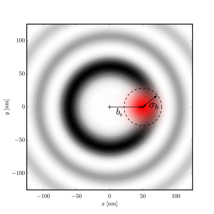
Figure 2: Illustration of a localized atomic target of size $\sigma_{b}$ that is displaced by the impact vector $b_{0}$ with regard to the center of the vortex beam.

II.4.2 Localized targets

Another (localized) target refers to a small cloud of atoms that is centered around the impact vector $\boldsymbol{b}_{0}$ in a plane perpendicular to the beam axis. We here assume a normalized Gaussian distribution of target atoms

$$\rho(\boldsymbol{b})=\frac{1}{\sqrt{2\pi}\sigma_{b}}\exp\left\{-\frac{(\boldsymbol{b}-\boldsymbol{b}_{0})^{2}}{2\sigma_{b}^{2}}\right\}\,$$ (30)

where $\sigma_{b}$ denotes the (r.m.s.) size of the target, cf. Fig. 2. Without loss of generality, moreover, we may assume that the impact vector $\boldsymbol{b}_{0}=b_{0}\boldsymbol{e}_{x}$ defines the $x$-axis and, hence, the angle $\varphi_{p}$ in the angular distribution of the photoelectrons below (and with the $z$-axis along the beam). For such a localized target with distribution $\rho(\boldsymbol{b})$, the partial photoionization probability becomes

$$\mathbb{P}^{(\ell)}_{\rho}(\boldsymbol{p}) =\int\!{{\mathrm{d}}^{2}\boldsymbol{b}}\,\rho(\boldsymbol{b})\>\mathbb{P}_{\boldsymbol{b}}^{(\ell)}(\boldsymbol{p})\,,$$ (31)

and where the integration over the target distribution below will be performed numerically.

II.5 Dichroism in two-color fields

In the previous section, we saw how the partial photoionization probabilities (25), (29) and (31) describe the yield of photoelectrons for a given sideband, as a function of the two emission angles $\vartheta_{p}$ and $\varphi_{p}$ for different kinds of targets. Of course, these probabilities also depend on the spin- and orbital angular momenta of the incident XUV and assisting NIR laser fields. To further understand how the coupling of these angular momenta affects the relative photoionization probabilities, we may resort to different kinds of dichroism signals as often used in describing the interaction of light with atoms, molecules and solids Kazansky et al. (2011); Mazza et al. (2014); Lux et al. (2012).

II.5.1 Circular dichroism for plane-waves

Let us start from the (atomic) circular dichroism which has been frequently used in characterizing the photoelectron emission if both, the XUV and the assisting NIR fields are described by plane waves. For two plane waves, as shown in Sect. II.3.2, the two-color ATI amplitude (15) and, hence, the corresponding photoionization probability only depends on the product of the two spin angular momentum (SAM) projections, i.e. the helicities of the XUV and laser photons. While there are four possible combinations of these helicities, only two $\Lambda_{X}\Lambda_{L}\>=\>\pm 1$ are distinguishable from each other. For the interaction of atoms with two plane waves, we can therefore define just one dichroism signal,

$$\mathrm{CD}=\frac{\mathbb{P}({\boldsymbol{p}};\Lambda_{X},\Lambda_{L})\;-\;\mathbb{P}(\boldsymbol{p};\Lambda_{X},-\Lambda_{L})}{\mathbb{P}(\boldsymbol{p};\Lambda_{X},\Lambda_{L})\>+\>\mathbb{P}(\boldsymbol{p};\Lambda_{X},-\Lambda_{L})}\,,$$ (32)

commonly known also as circular dichroism Kazansky et al. (2012), and which is a function of the photoelectron emission angles $\vartheta_{p}$ and $\varphi_{p}$, respectively. This circular dichroism can be defined uniquely for each sideband as long as the incident light beams are sufficiently monochromatic.

Table 1: Definition of the seven dichroism signals for the two-color ionization of atoms by a vortex (Bessel) beam and a plane-wave laser field.

Dichroism due to a flip of …		Definition
the helicity of the assisting NIR laser field.		$\displaystyle\mathcal{D}^{(\Lambda_{L})}$	$=$	$\frac{\mathbb{P}(\boldsymbol{p},m,\Lambda_{X},\Lambda_{L})-\mathbb{P}(\boldsymbol{p},m,\Lambda_{X},-\Lambda_{L})}{\mathbb{P}(\boldsymbol{p},m,\Lambda_{X},\Lambda_{L})+\mathbb{P}(\boldsymbol{p},m,\Lambda_{X},-\Lambda_{L})}$
the helicity of the XUV photons.		$\displaystyle\mathcal{D}^{(\Lambda_{X})}$	$=$	$\frac{\mathbb{P}(\boldsymbol{p},m,\Lambda_{X},\Lambda_{L})-\mathbb{P}(\boldsymbol{p},m,-\Lambda_{X},\Lambda_{L})}{\mathbb{P}(\boldsymbol{p},m,\Lambda_{X},\Lambda_{L})+\mathbb{P}(\boldsymbol{p},m,-\Lambda_{X},\Lambda_{L})}$
the projection of the orbital angular momentum.		$\displaystyle\mathcal{D}^{(m)}$	$=$	$\frac{\mathbb{P}(\boldsymbol{p},m,\Lambda_{X},\Lambda_{L})-\mathbb{P}(\boldsymbol{p},-m,\Lambda_{X},\Lambda_{L})}{\mathbb{P}(\boldsymbol{p},m,\Lambda_{X},\Lambda_{L})+\mathbb{P}(\boldsymbol{p},-m,\Lambda_{X},\Lambda_{L})}$
the helicity and the orbital angular momentum of the XUV Bessel beam. This is equivalent to just a flip of the projection of the total angular momentum.		$\displaystyle\mathcal{D}^{(m\Lambda_{X})}$	$=$	$\frac{\mathbb{P}(\boldsymbol{p},m,\Lambda_{X},\Lambda_{L})-\mathbb{P}(\boldsymbol{p},-m,-\Lambda_{X},\Lambda_{L})}{\mathbb{P}(\boldsymbol{p},m,\Lambda_{X},\Lambda_{L})+\mathbb{P}(\boldsymbol{p},-m,-\Lambda_{X},\Lambda_{L})}$
the helicities of both the laser and XUV photons. For two plane waves this dichroism signal is always zero because of the symmetry.		$\displaystyle\mathcal{D}^{(\Lambda_{X}\Lambda_{L})}$	$=$	$\frac{\mathbb{P}(\boldsymbol{p},m,\Lambda_{X},\Lambda_{L})-\mathbb{P}(\boldsymbol{p},m,-\Lambda_{X},-\Lambda_{L})}{\mathbb{P}(\boldsymbol{p},m,\Lambda_{X},\Lambda_{L})+\mathbb{P}(\boldsymbol{p},m,-\Lambda_{X},-\Lambda_{L})}$
the projection of the orbital angular momentum of the Bessel beam and of the helicity of the laser field.		$\displaystyle\mathcal{D}^{(m\Lambda_{L})}$	$=$	$\frac{\mathbb{P}(\boldsymbol{p},m,\Lambda_{X},\Lambda_{L})-\mathbb{P}(\boldsymbol{p},-m,\Lambda_{X},-\Lambda_{L})}{\mathbb{P}(\boldsymbol{p},m,\Lambda_{X},\Lambda_{L})+\mathbb{P}(\boldsymbol{p},-m,\Lambda_{X},-\Lambda_{L})}$
all three projections of the angular momenta simultaneously.		$\displaystyle\mathcal{D}^{(m\Lambda_{X}\Lambda_{L})}$	$=$	$\frac{\mathbb{P}(\boldsymbol{p},m,\Lambda_{X},\Lambda_{L})-\mathbb{P}(\boldsymbol{p},-m,-\Lambda_{X},-\Lambda_{L})}{\mathbb{P}(\boldsymbol{p},m,\Lambda_{X},\Lambda_{L})+\mathbb{P}(\boldsymbol{p},-m,-\Lambda_{X},-\Lambda_{L})}$

II.5.2 Dichroism signals for (vortex) Bessel beams

For vortex Bessel beams, the photoionization probability depends not only on the SAM of the XUV ($\Lambda_{X}=\pm 1$) and laser beams ($\Lambda_{L}=\pm 1$) but also on the orbital angular momentum $\pm m$ of the XUV photons. With three angular momenta, we can form eight combinations of $(m,\Lambda_{X},\Lambda_{L})$ by just changing the sign of one or more of these quantum numbers. This enables us to define seven different dichroism signals for the two-color ionization of atoms by a vortex and a plane-wave beam since one of the combinations, $\mathbb{P}(\boldsymbol{p},|m|,\Lambda_{X}=+1,\Lambda_{L}=+1)$, should occur as reference. For example, the dichroism that is associated with a flip of the projection of the orbital angular momentum $\pm m$ is easily defined by

$$\mathcal{D}^{(m)} =\frac{\mathbb{P}(\boldsymbol{p},m,\Lambda_{X},\Lambda_{L})\>-\>\mathbb{P}(\boldsymbol{p},-m,\Lambda_{X},\Lambda_{L})}{\mathbb{P}(\boldsymbol{p},m,\Lambda_{X},\Lambda_{L})\>+\>\mathbb{P}(\boldsymbol{p},-m,\Lambda_{X},\Lambda_{L})}\,.$$ (33)

Very similarly, we can define all the other dichroism signals as associated with some flip in the helicity and/or OAM quantum numbers, and which are displayed explicitly in Table 1 . As for the circular dichroism, all these (seven) dichroism signals generally depend for a localized target on the photoelectron emission angles $\vartheta_{p}$ and $\varphi_{p}$ as well as on the particular sideband $\ell$.

For sufficiently extended targets ($\sigma_{b}\varkappa\gg 1$), however, the photoionization probability and, hence, the dichroism signals above become independent of the (projection of the) orbital angular momentum or topological charge, $m$. This can be seen for instance from the analytical expression for the photoionization probability for infinitely extended targets (29), which is independent of $m$. For large targets, therefore, all the dichroism signals will depend just on the product $\Lambda_{X}\>\Lambda_{L}$ of the two helicities and, thus, all signals with $\Lambda_{X}\>\Lambda_{L}\>=\>+1$ must vanish in this limit, $\mathcal{D}^{(\Lambda_{X}\Lambda_{L})}=\mathcal{D}^{(m\Lambda_{X}\Lambda_{L})}=\mathcal{D}^{(m)}=0$. Moreover, all other signals with $\Lambda_{X}\>\Lambda_{L}\>=\>-1$ then coincide with the usual circular dichroism, $\mathcal{D}^{(\Lambda_{L})}=\mathcal{D}^{(\Lambda_{X})}=\mathcal{D}^{(m\Lambda_{X})}=\mathcal{D}^{(m\Lambda_{L})}$, cf. Eq. (32). For extended targets, a nonzero dichroism signal can be observed only if just one of the helicities $\Lambda_{X}$ or $\Lambda_{L}$ is changed.

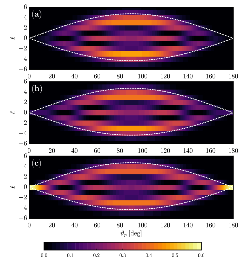
Figure 3: (Color online). Contourplot of the two-color ATI photoionization probability $\mathbb{P}^{(\ell)}(\vartheta_{p})$ as function of the emission angle $\vartheta_{p}$ and the sideband number $\ell$, i.e. the net number of absorbed or emitted laser photons by the outgoing photoelectrons. Results, encoded by colors (gray scale), are given for an infinitely extended target and are shown for (a) a plane-wave XUV beam as well as (b,c) a XUV Bessel beam with cone opening angles $\vartheta_{k}=0.2$ rad and $\vartheta_{k}=0.5$ rad, respectively. All these probabilities are independent of the topological charge $m$ of the Bessel beams because of the target size. The calculations were performed for the XUV frequency $\omega_{X}=3\,{\rm a.u.}=$81.6\text{\,}\mathrm{eV}$$ as well as for an assisting NIR laser field with frequency $\omega_{L}={0.05}\,{\rm a.u.}=$1.36\text{\,}\mathrm{eV}$$ and amplitude $A_{L}=0.1$ of the vector potential.

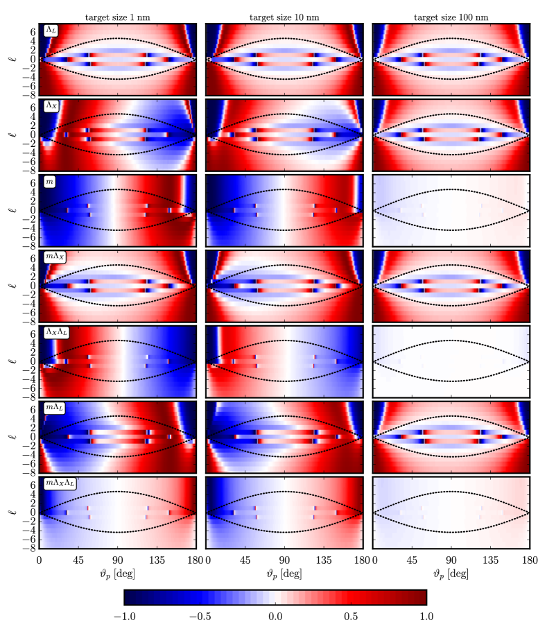
Figure 4: (Color online). Contourplot of the dichroism as function of the emission angle $\vartheta_{p}$ and the sideband number $\ell$ of the emitted electrons. Results are shown for the seven dichroism signals from Table  1 (rows 1-7), encoded by colors, and for the three target sizes $\sigma_{b}=$1\text{\,}\mathrm{nm}$$ (left column), $\sigma_{b}=$10\text{\,}\mathrm{nm}$$ (middle column) and $\sigma_{b}=$100\text{\,}\mathrm{nm}$$ (right column), respectively. The photoelectrons are observed at the azimuthal angle $\varphi_{p}=$90\text{\,}\mathrm{\SIUnitSymbolDegree}$$ with respect to the impact vector $b_{0}=$30\text{\,}\mathrm{nm}$$ as center of the target. All calculations were performed for a Bessel beam with photon energy $\omega_{X}={3}\,{\rm a.u.}=$81.6\text{\,}\mathrm{eV}$$, opening angle $\vartheta_{k}=0.2$ and orbital angular momentum projection $m=4$. The black dotted curves indicate the cut-off values of the number of sidebands as given analytically by Eq. (13).

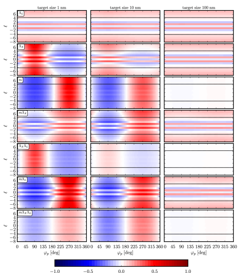
Figure 5: (Color online). The same as figure 4 but as function of the azimuthal angle $\varphi_{p}$ and for a Bessel beams with photon energy $\omega_{X}={5}\,{\rm a.u.}=$136\text{\,}\mathrm{eV}$$. Here, the photoelectrons are observed under the polar angle $\vartheta_{p}=$45\text{\,}\mathrm{\SIUnitSymbolDegree}$$ with regard to the beam axis and for a impact parameter $b_{0}=$25\text{\,}\mathrm{nm}$$.

III Results and Discussion

In the last section, we have analyzed the transition amplitude and photoionization probability for the two-color ATI of atoms by a vortex (Bessel) beam and combined with an intense plane-wave (NIR) laser field. Emphasize was placed here on the evaluation of this amplitude and the sideband structure of the central photoline due to the interaction of the emitted electrons with the NIR field. We also introduced various dichroism signals by flipping the projections of the spin and orbital angular momenta of the involved fields in order to quantify the dependence of the photoionization probability upon the angular momentum properties of the incident light beams.

As discussed above, the two-color ATI probability crucially depends for Bessel beams also on the size of the atomic target. To better understand the influence of this target size, detailed computations were performed for the photoionization of the $4s$ valence electron of Ca⁺ ions with binding energy $E_{B}=$11.7\text{\,}\mathrm{eV}$={0.43}\,{\rm a.u.}$. Simple core-Hartree wave functions in a screened potential have been applied to calculate all the necessary (one-electron) atomic matrix elements Fritzsche (2012), cf. (20).

In Fig. 3, we display the two-color ATI probability $\mathbb{P}^{(\ell)}(\vartheta_{p})$ as function of the emission angle $\vartheta_{p}$ (horizontal axis) and the sideband number $\ell$ (vertical axis). The sideband $\ell$ gives directly the net number of laser photons from the NIR field that are either absorbed or emitted by the outgoing photoelectrons. The ATI probabilities are encoded by colors and are shown for an infinitely extended target. Results are compared for the two-color ATI by a plane-wave XUV beam (upper panel) as well as for a XUV Bessel beam with cone opening angles $\vartheta_{k}=0.2$ rad (middle panel) and $\vartheta_{k}=0.5$ rad (lower panel), respectively. In these computations, we applied a XUV beam with the rather high frequency $\omega_{X}=3\,{\rm a.u.}=$81.6\text{\,}\mathrm{eV}$$ and for a NIR laser field with $\omega_{L}={0.05}\,{\rm a.u.}=$1.36\text{\,}\mathrm{eV}$$ and amplitude $A_{L}=0.1$. As seen from Fig. 3, the photoelectron distributions exhibit an almond-like shape for which the largest number of sidebands occurs at $\vartheta_{p}\,\simeq\,$90\text{\,}\mathrm{\SIUnitSymbolDegree}$$, while only the main photoline ($\ell=0$) is seen along the beam axis, i.e. for $\vartheta=$0\text{\,}\mathrm{\SIUnitSymbolDegree}$$ and $180\text{\,}\mathrm{\SIUnitSymbolDegree}$. This shape of the photoelectron distributions is well predicted also by the semiclassical cutoffs, Eq. (13), as indicated by the white dotted curves in the figures.

For the two-color ATI by a plane-wave XUV beam, the calculated photoelectron distribution agrees qualitatively well with the calculations by Kazansky and coworkers Kazansky et al. (2012). While no photoelectrons are seen in this case along the axis for plane-waves [cf. Fig. 3 a], this changes in the case of a twisted Bessel XUV beams in Figs. 3 b,c. For such Bessel beams, the photoionization probabilities along the beam axis increases with the cone opening angle $\vartheta_{k}$. We note that the plane-wave result is of course recovered in the paraxial approximation for $\vartheta_{k}\to 0$.

To analyze the localization effects of the target, we use the different dichroism signals as defined in Section II.5 and Table 1. Figure 4, for example, shows these dichroism signals as function of the emission angle $\vartheta_{p}$ and sideband number $\ell$ of the emitted electrons, and with the magnitude of the signals encoded by colors in the (seven) rows of the figure. We here applied a Bessel beam of the same frequency $\omega_{X}=$81.6\text{\,}\mathrm{eV}$$ and opening angle $\vartheta_{k}=0.2$ as in Fig. 3, and with the projection of the angular momentum $m=4$. Detailed computations are carried out for the three target sizes $\sigma_{b}=$1\text{\,}\mathrm{nm}$$ (left column), $\sigma_{b}=$10\text{\,}\mathrm{nm}$$ (middle column) and $\sigma_{b}=$100\text{\,}\mathrm{nm}$$ (right column), and for photoelectrons that are observed at the azimuthal angle $\varphi_{p}=$90\text{\,}\mathrm{\SIUnitSymbolDegree}$$ with regard to the impact vector $\boldsymbol{b}_{0}=b_{0}\,\boldsymbol{e}_{x}$ with $b_{0}=$30\text{\,}\mathrm{nm}$$ as the center of the target. While all the dichroism signals are quite different from each other for a small target (left column) and, hence, sensitive to the particular localization of the target, these differences become less pronounced as the target size increases. For target sizes (much) larger than the typical width of the rings in the Bessel beam, moreover, the dichroism signals approach the two limits: They either vanish identically if the product of the helicities of the two-color field is positive, $\Lambda_{X}\>\Lambda_{L}\>=\>+1$ [cf. the right panels of rows 3, 5 and 7], or these signals coincide with the known circular dichroism for $\Lambda_{X}\>\Lambda_{L}\>=\>-1$ [cf. the right panels of rows 1, 2, 4, and 6]. Let us note also that the (usual) circular dichroism signal in row 1 appears to be rather insensitive to the size of the target. In fact, these dichroism signals do not depend much on the details of the applied matrix elements as, in the electric-dipole approximation, the prefactor in Eq. (23) cancel in the ratio that is formed by any dichroism. Finally, the black dotted curves indicate the cut-off values of the number of sidebands as given analytically by Eq. (13). That means, while we can calculate a dichroism signal also outside the almond-shaped area, its measurement might be challenging since the photoionization probability is very small in these regions, cf. Fig. 3.

Due to the phase of the XUV Bessel beam, a localization of the target affects not only the (polar) angular emission of the photoelectrons but may results also in a non-trivial azimuthal distribution. Therefore, Fig. 5 shows the same as Fig. 4 but here as function of the azimuthal angle $\varphi_{p}$ and for a Bessel beams with slightly higher photon energy $\omega_{X}={5}\,{\rm a.u.}=$136\text{\,}\mathrm{eV}$$ and for a target centered at $b_{0}=$25\text{\,}\mathrm{nm}$$. In this figure, the photoelectrons are assumed to be observed under the polar angle $\vartheta_{p}=$45\text{\,}\mathrm{\SIUnitSymbolDegree}$$ with regard to the beam axis. An azimuthal anisotropy of the ATI probabilities is found for the localized targets as it was obtained before for the azimuthal distribution of photoelectrons Matula et al. (2013). This anisotropy of the ionization probabilities occurs of course also in the dichroism signals, while no azimuthal dependence appears for the usual circular dichroism (first row). As for the polar-angle dependence in Fig. 4, all dichroism signals become either zero or simply approach the circular dichroism for sufficiently large targets.

IV Summary and Conclusions

In this work, we investigated the two-color ATI of atoms and ions if light from a weak XUV Bessel beam is combined with a strong NIR laser field. While the emission of photoelectron occurs due to the weak XUV beam, the energy and angular distribution of the photoelectrons is affected by the plane-wave NIR field due to a net absorption or emission of one or several laser photons. Thus, the interaction of the atoms with such a two-color field results in sidebands to the normal photoline which are affected not only by the intensity and temporal structure of the NIR field but also by the location and extent of the atomic target as well as by the spin and orbital angular momenta of the two fields involved.

Emphasis in our analysis has been placed upon the energy spectra and angular emission of the photoelectrons as well as on the asymmetry in the photoelectron spectra if some of the SAM or OAM components of the fields are flipped relative to each other. For a XUV Bessel beam and a plane-wave NIR field, seven different dichroism signals can be defined. These signals differ for localized target but become either zero or coincide with the usual circular dichroism for macroscopically extended targets, similar as for Bessel beams with small opening angle. Our investigation of two-color strong field ATI with XUV vortex Bessel beams and the discussion of the seven different dichroism signals opens up avenues for future investigations of the interaction of atomic and molecular targets with twisted light in the high-intensity regime.

V Acknowledgments

This work was supported by the DFG priority programme 1840, ”Quantum Dynamics in Tailored Intense Fields”.

References

- Corkum and Krausz (2007) P. B. Corkum and Ferenc Krausz, “Attosecond science,” Nat. Phys. 3, 381 (2007).
- Krausz and Ivanov (2009) F. Krausz and M. Ivanov, “Attosecond physics,” Rev. Mod. Phys. 81, 163–234 (2009).
- Pazourek et al. (2015) R. Pazourek, S. Nagele, and J. Burgdörfer, “Attosecond chronoscopy of photoemission,” Rev. Mod. Phys. 87, 765–802 (2015).
- Gilbertson et al. (2010) S. Gilbertson, M. Chini, X. Feng, S. Khan, Y. Wu, and Z. Chang, “Monitoring and controlling the electron dynamics in helium with isolated attosecond pulses.” Phys. Rev. Lett. 105, 263003 (2010).
- Feist et al. (2009) J. Feist, S. Nagele, R. Pazourek, E. Persson, B. I. Schneider, L. A. Collins, and J. Burgdörfer, “Probing electron correlation via attosecond XUV pulses in the two-photon double ionization of helium.” Phys. Rev. Lett. 103, 063002 (2009).
- Haessler et al. (2010) S. Haessler, J. Caillat, W. Boutu, C. Giovanetti-Teixeira, T. Ruchon, T. Auguste, Z. Diveki, P. Breger, A. Maquet, B. Carré, R. Taïeb, and P. Salières, “Attosecond imaging of molecular electronic wavepackets,” Nat. Phys. 6, 200–206 (2010).
- Cavalieri et al. (2007) A. L. Cavalieri, N. Müller, Th. Uphues, V. S. Yakovlev, A. Baltuška, B. Horvath, B. Schmidt, L. Blümel, R. Holzwarth, S. Hendel, M. Drescher, U. Kleineberg, P. M. Echenique, R. Kienberger, F. Krausz, and U. Heinzmann, “Attosecond spectroscopy in condensed matter,” Nature 449, 1029–1032 (2007).
- Krüger et al. (2012) M. Krüger, M. Schenk, M. Förster, and P. Hommelhoff, “Attosecond physics in photoemission from a metal nanotip,” J. Phys. B At. Mol. Opt. Phys. 45, 074006 (2012).
- Sansone et al. (2006) G. Sansone, E. Benedetti, F. Calegari, C. Vozzi, L. Avaldi, R. Flammini, L. Poletto, P. Villoresi, C. Altucci, R. Velotta, S. Stagira, S. De Silvestri, and M. Nisoli, “Isolated Single-Cycle Attosecond Pulses,” Science 314, 443 (2006).
- Popmintchev et al. (2012) T. Popmintchev, M.-C. Chen, D. Popmintchev, P. Arpin, S. Brown, S. Ališauskas, G. Andriukaitis, T. Balčiunas, O. D. Mücke, A. Pugzlys, A. Baltuška, B. Shim, S. E. Schrauth, A. Gaeta, C. Hernández-García, L. Plaja, A. Becker, A. Jaron-Becker, M. M. Murnane, and H. C. Kapteyn, “Bright Coherent Ultrahigh Harmonics in the keV X-ray Regime from Mid-Infrared Femtosecond Lasers,” Science 336, 1287 (2012).
- Calegari et al. (2016) F. Calegari, G. Sansone, S. Stagira, C. Vozzi, and M. Nisoli, “Advances in attosecond science,” J. Phys. B At. Mol. Opt. Phys. 49, 062001 (2016).
- Milošević et al. (2006) D. B. Milošević, G. G. Paulus, D. Bauer, and W. Becker, “Above-threshold ionization by few-cycle pulses,” J. Phys. B 39, R203 (2006).
- Wittmann et al. (2009) T. Wittmann, B. Horvath, W. Helml, M. G. Schätzel, X. Gu, A. L. Cavalieri, G. G. Paulus, and R. Kienberger, “Single-shot carrier-envelope phase measurement of few-cycle laser pulses,” Nat. Phys. 5, 357–362 (2009).
- Ehlotzky (2001) F. Ehlotzky, “Atomic phenomena in bichromatic laser fields,” Phys. Rep. 345, 175 (2001).
- Radcliffe et al. (2012) P. Radcliffe, M. Arbeiter, W. B. Li, S. Düsterer, H. Redlin, P. Hayden, P. Hough, V. Richardson, J. T. Costello, T. Fennel, and M. Meyer, “Atomic photoionization in combined intense XUV free-electron and infrared laser fields,” New J. Phys. 14, 043008 (2012).
- Muller et al. (1986) H. G. Muller, H. B. van Linden van den Heuvell, and M. J. van der Wiel, “Dressing of continuum states and MPI of Xe in a two-colour experiment,” J. Phys. B At. Mol. Phys. 19, L733 (1986).
- Schins et al. (1994) J. M. Schins, P. Breger, P. Agostini, R. C. Constantinescu, H. G. Muller, G. Grillon, A. Antonetti, and A. Mysyrowicz, “Observation of laser-assisted Auger decay in argon.” Phys. Rev. Lett. 73, 2180–2183 (1994).
- Glover et al. (1996) T. E. Glover, R. W. Schoenlein, A. H. Chin, and C. V. Shank, “Observation of laser assisted photoelectric effect and femtosecond high order harmonic radiation.” Phys. Rev. Lett. 76, 2468–2471 (1996).
- Meyer et al. (2006) M. Meyer, D. Cubaynes, P. O’Keeffe, H. Luna, P. Yeates, E. T. Kennedy, J. T. Costello, P. Orr, R. Taïeb, A. Maquet, S. Düsterer, P. Radcliffe, H. Redlin, A. Azima, E. Plönjes, and J. Feldhaus, “Two-color photoionization in xuv free-electron and visible laser fields,” Phys. Rev. A 74, 011401 (2006).
- Meyer et al. (2008) M. Meyer, D. Cubaynes, D. Glijer, J. Dardis, P. Hayden, P. Hough, V. Richardson, E. T. Kennedy, J. T. Costello, P. Radcliffe, S. Düsterer, A. Azima, W. B. Li, H. Redlin, J. Feldhaus, R. Taïeb, A. Maquet, A. N. Grum-Grzhimailo, E. V. Gryzlova, and S. I. Strakhova, “Polarization control in two-color above-threshold ionization of atomic helium.” Phys. Rev. Lett. 101, 193002 (2008).
- Meyer et al. (2010) M. Meyer, D. Cubaynes, V. Richardson, J. T. Costello, P. Radcliffe, W. B. Li, S. Düsterer, S. Fritzsche, A. Mihelic, K. G. Papamihail, and P. Lambropoulos, “Two-photon excitation and relaxation of the 3d-4d resonance in atomic Kr.” Phys. Rev. Lett. 104, 213001 (2010).
- Helml et al. (2014) W. Helml, A. R. Maier, W. Schweinberger, I. Grguraš, P. Radcliffe, G. Doumy, C. Roedig, J. Gagnon, M. Messerschmidt, S. Schorb, C. Bostedt, F. Grüner, L. F. DiMauro, D. Cubaynes, J. D. Bozek, Th. Tschentscher, J. T. Costello, M. Meyer, R. Coffee, S. Düsterer, A. L. Cavalieri, and R. Kienberger, “Measuring the temporal structure of few-femtosecond free-electron laser X-ray pulses directly in the time domain,” Nature Photonics 8, 950–957 (2014).
- Leitner et al. (2015) T. Leitner, R. Taïeb, M. Meyer, and P. Wernet, “Probing photoelectron angular distributions in molecules with polarization-controlled two-color above-threshold ionization,” Phys. Rev. A 91, 063411 (2015).
- O’Keeffe et al. (2004) P. O’Keeffe, R. López-Martens, J. Mauritsson, A. Johansson, A. L’Huillier, V. Véniard, R. Taïeb, A. Maquet, and M. Meyer, “Polarization effects in two-photon nonresonant ionization of argon with extreme-ultraviolet and infrared femtosecond pulses,” Phys. Rev. A 69, 051401 (2004).
- Guyétand et al. (2005) O. Guyétand, M. Gisselbrecht, A. Huetz, P. Agostini, R. Taïeb, V. Véniard, A. Maquet, L. Antonucci, O. Boyko, C. Valentin, and D. Douillet, “Multicolour above-threshold ionization of helium: quantum interference effects in angular distributions,” J. Phys. B At. Mol. Opt. Phys. 38, L357–L363 (2005).
- Kazansky et al. (2012) A. K. Kazansky, A. V. Grigorieva, and N. M. Kabachnik, “Dichroism in short-pulse two-color XUV plus IR multiphoton ionization of atoms,” Phys. Rev. A 85, 053409 (2012).
- Kazansky et al. (2011) A. K. Kazansky, A. V. Grigorieva, and N. M. Kabachnik, “Circular dichroism in laser-assisted short-pulse photoionization.” Phys. Rev. Lett. 107, 253002 (2011).
- Mazza et al. (2014) T. Mazza, M. Ilchen, A. J. Rafipoor, C. Callegari, P. Finetti, O. Plekan, K. C. Prince, R. Richter, M. B. Danailov, A. Demidovich, G. De Ninno, C. Grazioli, R. Ivanov, N. Mahne, L. Raimondi, C. Svetina, L. Avaldi, P. Bolognesi, M. Coreno, P. O’Keeffe, M. Di Fraia, M. Devetta, Y. Ovcharenko, Th. Möller, V. Lyamayev, F. Stienkemeier, S. Düsterer, K. Ueda, J. T. Costello, A. K. Kazansky, N. M. Kabachnik, and M. Meyer, “Determining the polarization state of an extreme ultraviolet free-electron laser beam using atomic circular dichroism,” Nat. Commun. 5, 3648 (2014).
- Guyétand et al. (2008) O. Guyétand, M. Gisselbrecht, A. Huetz, P. Agostini, R. Taïeb, A. Maquet, B. Carré, P. Breger, O. Gobert, D. Garzella, J.-F. Hergott, O. Tcherbakoff, H. Merdji, M. Bougeard, H. Rottke, M. Böttcher, Z. Ansari, and P. Antoine, “Evolution of angular distributions in two-colour, few-photon ionization of helium,” J. Phys. B At. Mol. Opt. Phys. 41, 051002 (2008).
- Lux et al. (2012) Ch. Lux, M. Wollenhaupt, T. Bolze, Q. Liang, J. Köhler, C. Sarpe, and Th. Baumert, “Circular Dichroism in the Photoelectron Angular Distributions of Camphor and Fenchone from Multiphoton Ionization with Femtosecond Laser Pulses,” Angew. Chemie Int. Ed. 51, 5001–5005 (2012).
- Molina-Terriza et al. (2007) G. Molina-Terriza, J. P. Torres, and L. Torner, “Twisted photons,” Nat. Phys. 3, 305–310 (2007).
- Stock et al. (2015) S. Stock, A. Surzhykov, S. Fritzsche, and D. Seipt, “Compton scattering of twisted light: Angular distribution and polarization of scattered photons,” Phys. Rev. A 92, 013401 (2015), arXiv:1505.00313 .
- Quinteiro et al. (2015) G. F. Quinteiro, D. E. Reiter, and T. Kuhn, “Formulation of the twisted-light–matter interaction at the phase singularity: The twisted-light gauge,” Phys. Rev. A 91, 033808 (2015).
- Surzhykov et al. (2015) A. Surzhykov, D. Seipt, V. G. Serbo, and S. Fritzsche, “Interaction of twisted light with many-electron atoms and ions,” Phys. Rev. A 91, 013403 (2015).
- Schmiegelow et al. (2016) Ch. T. Schmiegelow, J. Schulz, H. Kaufmann, T. Ruster, U. G. Poschinger, and F. Schmidt-Kaler, “Transfer of optical orbital angular momentum to a bound electron,” Nature Communications 7, 12998 (2016).
- Radwell et al. (2015) N. Radwell, T. W. Clark, B. Piccirillo, S. M. Barnett, and S. Franke-Arnold, “Spatially dependent electromagnetically induced transparency.” Phys. Rev. Lett. 114, 123603 (2015).
- Bozinovic et al. (2013) N. Bozinovic, Y. Yue, Y. Ren, M. Tur, P. Kristensen, H. Huang, A. E. Willner, and S. Ramachandran, “Terabit-Scale Orbital Angular Momentum Mode Division Multiplexing in Fibers,” Science 340, 1545 (2013).
- Krenn et al. (2014) M. Krenn, R. Fickler, M. Fink, J. Handsteiner, M. Malik, T. Scheidl, R. Ursin, and A. Zeilinger, “Communication with spatially modulated light through turbulent air across Vienna,” New J. Phys. 16, 113028 (2014).
- Volkov (1935) D. M. Volkov, “Über eine Klasse von Lösungen der Diracschen Gleichung,” Z. Phys. 94, 250 (1935).
- Hemsing et al. (2013) E. Hemsing, A. Knyazik, M. Dunning, D. Xiang, A. Marinelli, C. Hast, and J. B Rosenzweig, “Coherent optical vortices from relativistic electron beams,” Nat. Phys. 9, 549 (2013).
- Bahrdt et al. (2013) J. Bahrdt, K. Holldack, P. Kuske, R. Müller, M. Scheer, and P. Schmid, “First Observation of Photons Carrying Orbital Angular Momentum in Undulator Radiation,” Phys. Rev. Lett. 111, 034801 (2013).
- Zürch et al. (2012) M. Zürch, C. Kern, P. Hansinger, A. Dreischuh, and Ch. Spielmann, “Strong-field physics with singular light beams,” Nat. Phys. 8, 743 (2012).
- Gariepy et al. (2014) G. Gariepy, J. Leach, K. T. Kim, T. J. Hammond, E. Frumker, R. W. Boyd, and P. B. Corkum, “Creating High-Harmonic Beams with Controlled Orbital Angular Momentum,” Phys. Rev. Lett. 113, 153901 (2014).
- Hernández-García et al. (2013) C. Hernández-García, A. Picón, J. San Román, and L. Plaja, “Attosecond Extreme Ultraviolet Vortices from High-Order Harmonic Generation,” Phys. Rev. Lett. 111, 083602 (2013).
- Jentschura and Serbo (2011) U. D. Jentschura and V. G. Serbo, “Generation of High-Energy Photons with Large Orbital Angular Momentum by Compton Backscattering,” Phys. Rev. Lett. 106, 013001 (2011).
- Ivanov and Serbo (2011) I. P. Ivanov and V. G. Serbo, “Scattering of twisted particles: Extension to wave packets and orbital helicity,” Phys. Rev. A 84, 033804 (2011).
- Matula et al. (2013) O. Matula, A. G. Hayrapetyan, V. G. Serbo, A. Surzhykov, and S. Fritzsche, “Atomic ionization of hydrogen-like ions by twisted photons: angular distribution of emitted electrons,” J. Phys. B 46, 205002 (2013).
- Note (1) Note the different definition of the vector in Matula et al. (2013) which furnishes a different interpretation of the quantum number as the TAM eigenvalue of the Bessel beam, but without any physical consequences.
- Note (2) Strictly speaking, the orbital quantum number here refers to the dominant component of the three possible projections of the orbital angular momentum, and it coincides with the true OAM only in the paraxial limit .
- Watson (1922) G. N. Watson, A treatise on the theory of Bessel functions (Cambridge University Press, 1922).
- Lewenstein et al. (1994) M. Lewenstein, Ph. Balcou, M. Y. Ivanov, A. L’Huillier, and P. B. Corkum, “Theory of high-harmonic generation by low-frequency laser fields,” Phys. Rev. A 49, 2117 (1994).
- Zhang et al. (2013) K. Zhang, J. Chen, X.-L. Hao, P. Fu, Z.-C. Yan, and B. Wang, “Terracelike structure in the above-threshold-ionization spectrum of an atom in an IR+XUV two-color laser field,” Phys. Rev. A 88, 043435 (2013).
- Seipt et al. (2015) D. Seipt, S. G. Rykovanov, A. Surzhykov, and S. Fritzsche, “Narrowband inverse Compton scattering x-ray sources at high laser intensities,” Phys. Rev. A 91, 033402 (2015).
- Seipt et al. (2016) D. Seipt, A. Surzhykov, S. Fritzsche, and B. Kämpfer, “Caustic structures in x-ray Compton scattering off electrons driven by a short intense laser pulse,” New J. Phys. 18, 023044 (2016).
- Kazansky et al. (2010) A. K. Kazansky, I. P. Sazhina, and N. M. Kabachnik, “Angle-resolved electron spectra in short-pulse two-color XUV + IR photoionization of atoms,” Phys. Rev. A 82, 033420 (2010).
- Fritzsche (2012) S. Fritzsche, “The RATIP program for relativistic calculations of atomic transition, ionization and recombination properties,” Comput. Phys. Commun. 183, 1525 (2012).