Where is the Goldmine? Finding Promising Business Locations through Facebook Data Analytics

Abstract

If you were to open your own cafe, would you not want to effortlessly identify the most suitable location to set up your shop? Choosing an optimal physical location is a critical decision for numerous businesses, as many factors contribute to the final choice of the location. In this paper, we seek to address the issue by investigating the use of publicly available Facebook Pages data—which include user “check-ins”, types of business, and business locations—to evaluate a user-selected physical location with respect to a type of business. Using a dataset of 20,877 food businesses in Singapore, we conduct analysis of several key factors including business categories, locations, and neighboring businesses. From these factors, we extract a set of relevant features and develop a robust predictive model to estimate the popularity of a business location. Our experiments have shown that the popularity of neighboring business contributes the key features to perform accurate prediction. We finally illustrate the practical usage of our proposed approach via an interactive web application system.

1 Introduction

Motivation. Location is a crucial factor of retail success, as 94% of retail sales are still transacted in physical stores [24]. To increase the chance of success for their stores, business owners require not only the knowledge of where their potential customers are, but also their surrounding competitors and complementary businesses. From the property owners’ standpoint, it is also important to assess the potential success values of their property locations so as to determine the appropriate businesses to lease the locations to and for the right amounts. However, assessing and picking a store location is a cumbersome task for both business and property owners.

To carry out the above tasks well, many factors need to be taken into account, each of which requires gathering and analyzing the relevant data. Traditionally, business and property owners conduct surveys to assess the value of store locations [3]. Such surveys, however, are costly and do not scale up well. With fast changing environments (e.g., neighborhood rental, local population size, composition, etc.) and emergence of new business locations, one also needs to continuously reevaluate the value of store locations.

Fortunately, in the era of social media and mobile apps, we have an abundance of online user-generated data, which capture both activities of users in social media as well as offline activities at physical locations. Facebook is one of the world’s largest social media platforms, with more than 1 billion active users everyday [21]. From the business standpoint, the massive availability of user, location, and other behavioral data in Facebook is attractive, and has changed the way people do businesses. For instance, many small/medium business owners are now setting up Facebook Pages to: (i) allow customers to find their businesses on Facebook; (ii) connect with customers via “likes” and “check-ins”; (iii) reach out to more customers through advertising their business pages on Facebook; and (iv) conduct analytics of their pages to get a deeper understanding of their customers and marketing activities.

Consumers are also adapting both their online and offline behaviors to the introduction of Facebook Pages for businesses. Other than “liking” businesses on their Facebook Pages, they can do a “check-in” whenever they physically visit the respective business stores. Facebook Pages have turned many offline signals into online behavior that can be analyzed for business insights. In particular, features such as “likes” and “check-ins” can be used as indicators of popularity, and by extension, success. Similarly, Instagram, Twitter, and Foursquare also have variants of these quantitative signals that can be retrieved from their geotagged photos, tweets, and tips. These data allow us to study the dynamics of brick-and-mortar stores and discover meaningful patterns and insights that will help retail and property owners make better decisions.

Objective. In this work, we make use of data collected from Facebook Pages to answer important research questions such as: “Where should an owner set up his physical retail store at, so as to optimize the store’s popularity?”, “What are the important factors influencing a store’s popularity?”, and “Is there a “local” effect, whereby businesses can benefit from the presence of more popular/established neighbors?” To this end, we propose a new location analytics framework that operates on top of Facebook Pages data. The centerpiece of our current framework is the following prediction task: Given a target location that a business/property owner wants to hypothetically set his/her store at, how can we extract the relevant data of businesses within the vicinity of the target location and use them to estimate the popularity of the target location?

As an illustration, Figure 1 shows a visualization of our web application system that realizes our location analytics framework. For the system’s input, a business/property owner first drops a blue pin on the map that indicates the hypothetical location of his/her new store. Our system then retrieves the relevant information about the area nearby, which are also occupied by the existing businesses as indicated by the red pins. Based on these inputs, the system extracts a set of features and invokes a machine learning algorithm to predict the “check-in” score for the target location, which in turn serves as an indicator for the potential popularity of that location.

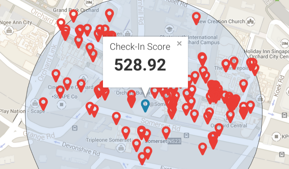
Figure 1: Prediction of “check-ins” based on the location indicated by the blue pin. The red pins represent nearby existing businesses.

Contributions. In this paper, we show how publicly available Facebook Pages data can be analyzed and used to predict the potential popularity of a business location. To our best knowledge, this is the first work that demonstrates the feasibility of using Facebook data for business location analytics and, in particular, for aiding business and property owners to evaluate the value of a store location. It is also worth noting that our work presents a fine-grained approach that allows the business/property owners to estimate the popularity of any point on the city map. Our approach can be easily extended to predict multiple points simultaneously as well. We summarize our main contributions as follows:

• We present a new study on business location analytics using Facebook Pages data. Specifically, we conduct detailed analyses on 20,877 Facebook Pages of food-related businesses in Singapore, which constitute one of the largest business types in the city with generally healthy visitor traffic. Based on the analyses, we identify key features that can be used to extract insights, as well as suitable metric for business popularity.

• We develop a location analytics framework that includes a rich feature extraction module as well as a fast and accurate predictive model based on gradient boosting machine (GBM) [8]. Unlike the previous close work on optimal store placement [13] that outputs a ranked list of discretized areas (circles) with fixed radius, our approach is much more fine-grained. That is, our model can estimate on the fly the popularity of any arbitrary point on the map—which can be the location of an existing or a new/hypothetical business—without needing the locations to be discretized a priori.

• Based on our (trained) predictive model, we analyze the contribution of key features that are crucial in predicting the popularity of a retail business—at both chunk (i.e., a group of features) and individual feature levels. In particular, we discover that distance-dependent features such as the total “check-ins” of businesses within certain radius are of utmost importance. We then provide an in-depth investigation on whether businesses, particularly smaller ones, benefit from the existence of other popular businesses within its vicinity.

• To concretely realize our idea, we have built an interactive web application that allows a business/property owner to drop a pin on the map and obtain a predicted “check-in” score for that location. The application is available at http://research.larc.smu.edu.sg/bizanalytics/.

Paper outline. Section 2 first provides an overview of related works. In Section 3, we describe the Singapore Facebook Pages data we use in our experiments. We subsequently elaborate our proposed location analytics approach in Section 4. Section 5 presents our experimental setup, followed by the results and analyses in Section 6. We present our web application prototype in Section 7, and finally conclude the paper in Section 8.

2 Related Work

Our work can be viewed as a new type of location analytics [11], which is an emerging area related to business intelligence (BI) [2]. In recent years, organizations have relied on BI tools to delve into their data and reveal key insights that can aid their decision-making processes. With these tools, businesses have been able to make informed decisions based on what happened and when — typically pertaining to sales figures and supplier transactions. Lately, there is an important trend for organizations to address the question of where. Conventional BI systems, however, lack location-related analytics capabilities, and thus do not consider geographic and demographic factors crucial for consumer analysis, e.g., where to set up stores, warehouses, or marketing campaigns.

Previously, combining separate BI and location-based approaches such as geographic information systems (GIS), was privileged only to large enterprises such as oil/gas-exploration companies, transportation companies, or government agencies [2]. These technologies involve costly data acquisition processes and specialized labor skills. Moreover, their integration requires complex and time-consuming implementation. A recent survey by ESRI and IT Media firm TechTarget [4] discovered that many organizations now believe that it is important to look at business data in a geographical context. Today, location-based data are abundant, thanks to the large volumes of user traces available from social media (such as Foursquare and Facebook) as well as mobile devices. However, many organizations are still unaware of the value of location-based data and struggle to put them to effective use.

Using data from social media to understand the dynamics of a society has always been a popular research theme, particularly, in recommending a new location to a user. For example, Facebook researchers Chang and Sun [1] analyzed Facebook users’ “check-ins” data to develop models that predict where users will “check-in” next. They were able to predict user-to-user friendships (i.e., friend recommendation) just by the “check-in” data alone. Gao et al. [9] explored the use of Foursquare “check-ins” and temporal effects for the task of location-recommendation; subsequently, the data were also used to predict a user’s location [10].

Recent works on social media-based location analytics largely focus on detecting events and predicting user mobility patterns, although their use for BI applications are still limited so far. For instance, Li et al. [14] presented a machine learning method to discover and profile the user’s location based on their following network and tweet contents. Noulas et al. [17] used Foursquare data to study the problem of predicting the next venue a mobile user will visit, by exploiting transitions between types of venues, mobility flows between venues, and spatio-temporal patterns of user “check-ins”. Also based on Foursquare data, Karamshuk et al. [13] demonstrated the power of geographic (e.g., types and density of nearby places) and user mobility (e.g., transitions between venues or incoming flow of users) features in predicting the best placement of retail stores. In a similar vein, Georgiev et al. [12] conducted a study to predict the rise and decline of popularity of the local retail shops during the 2012 London Olympic Games. Most recently, Zhang et al. [25] extracted traffic and human mobility features from Manhattan restaurants data and studied how static and dynamic factors affect the economic outcome of local businesses in the city.

Our approach. Our work differs from all the above studies in several ways. Firstly, to our best knowledge, our work is the first to explore the use of Facebook data in business-location analytics. With 1.55 billion monthly active users and 50 million business pages [21], Facebook can provide a more comprehensieve database of crowdsourced locations than other platforms (by comparison, Foursquare only has 55 million monthly active users and 1.3 million business pages [22]). Secondly, instead of recommending places for users to establish retail stores or analyze on how unique events will affect businesses,we predict the popularity score of a user-selected venue, giving the user more freedom to choose anywhere he/she wants to set up his/her business. Thirdly, among all the works, Karamshuk et al.’s [13] is the closest to ours. But the key difference is that their work discretized the city into multiple circles with fixed radius and treated the issue as a “ranking problem”, i.e., producing a ranked list of discretized circles. In contrast, we view it as a “prediction problem” and provides a much more fine-grained approach of estimating the popularity of any point on the map. Our method also works robustly on a range of radius values, instead of relying on a single predefined radius as in [13].

3 Facebook Pages Dataset

In this section, we first provide an overview of the data that we collected from Facebook, and then describe the important attributes found in the data. We then conduct a simple analysis on the two popularity measures—“check-ins” and “likes”—to determine the better metric for quantifying the popularity of a business.

3.1 Data Harvesting

In this paper, we focus our studies on food-related businesses found in the Facebook of Singapore. We choose food because it constitutes one of the largest business types in Singapore with generally healthy visitor traffic (“check-ins” and “likes”). The food-related businesses were defined based on a manually-curated list that consists of $133$ food-related categories of business, such as those containing the words “restaurant”, “pub”, “bar”, etc. In particular, we consider food-related businesses in Singapore Facebook Pages that explicitly specify latitute-longitude coordinates, and these coordinates must be within the physical boundaries of Singapore. Using Facebook’s Graph API [6], we obtained a total of 82,566 business profiles within Singapore boundaries, of which we categorically filtered 20,877 (25.2%) profiles that are food-related. All business data were analyzed in aggregate, and no personally-identifiable information was used.

Figure 2 shows an example of one such business profile, Wimbly Lu Chocolates, with important attributes (highlighted in bold) such as: (i) ID, (ii) category (i.e., the primary-category), (iii) category list (i.e., the sub-categories), (iv) “check-in” count, (v) “like” count, and (vi) location (including latitude and longitude). Figure 3 shows the corresponding Facebook Page of the business profile.

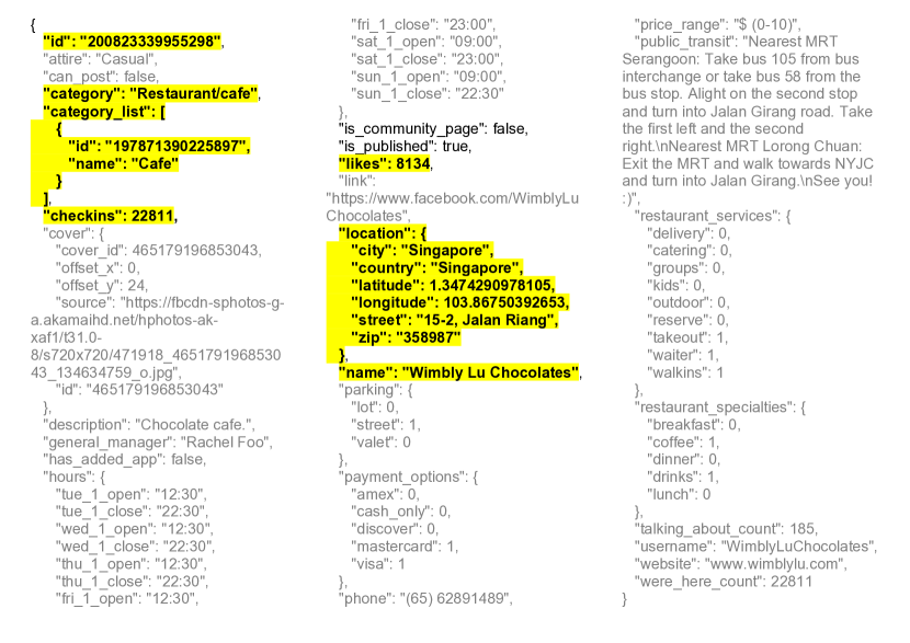
Figure 2: Facebook Graph API provides a JSON-formatted data of a business. Shown here is the Facebook Page of the Wimbly Lu Chocolates cafe in Singapore. Source: %Source:␣\href{https://graph.facebook.com/200823339955298/}{\texttt{https://graph.facebook.com/200823339955298/}}}https://graph.facebook.com/200823339955298/

Figure 3: The Facebook page of Wimbly Lu Chocolates that shows key popularity metrics such as 8.131 “likes” and 22K “check-ins”.

Table 1: Top 25 categories of food-businesses, their expected “check-ins”, and those that perform better than the expectation.

Categories	Businesses	Total “check-ins”	Expected “check-ins”	% of Businesses that have “check-ins”
	count		per business	above the expected “check-ins”
Food & Restaurant	6,758	5,771,148	853.97	13.36%
Restaurant	5,233	8,195,356	1,566.09	16.09%
Cafe	3,126	3,799,849	1,215.56	19.10%
Shopping Mall	3,101	5,772,105	1,861.37	15.90%
Coffee Shop	2,959	2,395,000	809.40	13.99%
Fast Food Restaurant	2,840	3,447,999	1,214.08	19.12%
Food & Grocery	1,449	1,055,175	728.21	6.21%
Bakery	1,338	394,982	295.20	11.58%
Chinese Restaurant	1,157	2,376,432	2,053.96	23.16%
Food Stand	1,099	1,454,820	1,323.77	10.92%
Bar	956	3,234,860	3,383.74	20.08%
Japanese Restaurant	922	1,297,228	1,406.97	22.02%
Train Station	879	429,740	488.90	26.17%
Nightlife	744	866,619	1,164.81	10.62%
Movie Theater	717	1,015,632	1,416.50	9.09%
Cafeteria	661	421,774	638.08	11.20%
Seafood Restaurant	629	1,786,933	2,840.91	22.58%
Italian Restaurant	459	735,620	1,602.66	27.67%
Thai Restaurant	437	593,546	1,358.23	26.32%
Ice Cream Parlor	413	744,514	1,802.70	18.40%
Sushi Restaurant	380	741,305	1,950.80	26.58%
Pub	369	513,009	1,390.27	20.33%
Night Club	361	1,416,278	3,923.21	14.40%
Indian Restaurant	350	538,624	1,538.93	18.00%

3.2 Categories Data

From the 20,877 food-related businesses, we retrieved a total of 357 unique categorical labels (as standardized by Facebook) from the attribute “category list”, which represents the sub-categories of a business. These categories contain not only food-related labels (i.e., “bakery”, “bar”, “cafe”, “coffee shop”), but also non-food labels such as “movie theatre”, “shopping mall”, and “train station.” The existence of non-food related labels within food businesses is Facebook’s way of allowing business owners to choose more than one categorical label for their business profile. For example, a Starbucks outlet located at a train station in an airport would likely have a mixture of food and non-food labels, such as “airport”, “cafe”, “coffee shop”, and “train station.” In addition, there is an intimate relationship between the categories of a target business and those of its neighbors. For instance, a family-run cafe will unlikely set itself next to an established coffee franchise like Starbucks, whereas a dessert shop may be located near complementary dining places.

Table 1 shows the top 25 categories of the food businesses in Singapore, their expected “check-ins”, and the percentage of businesses that perform better than expectation. The proportion of businesses performing better than expectation ranges from 6 to 28%. The largest category is “food and restaurant”, which is the most common category-type. From the low percentages of those that actually perform better than the expectation, we can tell that businesses obey a long-tail distribution, with the majority of businesses being unable to achieve the expected “check-ins” or more.

3.3 Location Data

Each business profile has a location attribute that contains the physical address and latitude-longitude coordinates (hereafter known as “lat-long”). Knowing the location of every business allows us to calculate the neighborhood of a selected business through the spatial distribution of other businesses around the vicinity. Specifically, we consider the set $P_{l}=\{p|dist(p,l)\leq r\}$ of places $p$ that lie in a radius $r$ around a target location $l$. The term $dist(p,l)$ denotes the Haversine distance [20] between two locations $p$ and $l$. We can then create a two-dimensional distance matrix containing the distance between every pair of business. For efficiency, we only consider a maximum radius of 1km (i.e., $r\leq 1$km). This allows us to quickly retrieve the $k$ nearest neighbors of any location.

3.4 Visitor Data

Ideally, we would like to analyze customer information, such as who commented on or “liked” a business’ Facebook post, and match/recommend some user profiles to some businesses. However, due to privacy concerns, Facebook does not allow us to identify who has checked-in or liked a particular business. Although one can still crawl the posts on a business’ wall, as of Facebook’s Graph API v2.0 [5] (released in 2014), Facebook no longer supplies a user’s actual ID. Instead, Facebook uses the concept of “app-scoped user IDs”, whereby a user’s ID is unique to each app and cannot be used across different apps. As our crawler is considered an app, and Facebook limits the number of user posts that an app can query in a day, we are unable to gather enough posts—and by extension user IDs—to cover all (food-related) businesses in Singapore. Having multiple crawlers will not work either, as the same user ID will be different for any two crawlers.

3.5 Popularity Indicator: “Check-in” vs “Like”

Facebook provides two possible indicators for a business page’s popularity: “check-in” and “like”. The “check-in” metric is common in location-based social media like Facebook and Foursquare. Meanwhile, the “like” metric (shown as a “thumbs up” button) is more unique to Facebook, allowing users to express their recommendation/support for an entity. A “check-in” is the action of registering one’s physical presence, and the total number of “check-ins” received by a business gives us a rough estimate of how popular and well-received it is. In contrast, the number of “likes” literally reflects an online vote for the business. Intuitively, therefore, a “check-in” should be a more suitable measure of a physical store’s popularity, as it indicates a physical presence. Furthermore, “check-in” can be repeated, i.e., a user could “check-in” to a place on Monday and do so again on Tuesday. By contrast, “likes” cannot be done repeatedly—it is a one-time event.

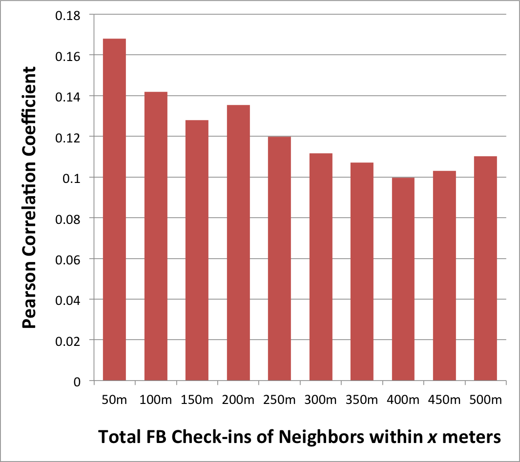
(a) Target business’ total “check-ins” vs. neighbors’ total checkins

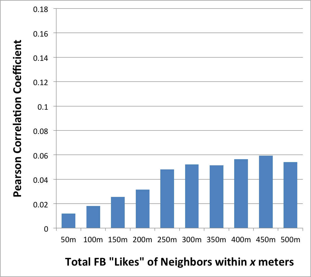
(b) Target business’ total “check-ins” vs. neighbors’ total likes

Figure 4: Pearson correlation coefficient (PCC) of neighboring total “check-ins” (in red) and neighboring total “likes” (in blue).

To prove this point, we compute the Pearson correlation coefficient (PCC) on two pairs: (i) the target business’ “check-ins” w.r.t. its neighbors’ total “check-ins”, and (ii) the target business’ “check-ins” w.r.t. its neighbors’ total “likes”. We only use the number of “check-ins” for the target business because we are only interested in the physical presence of customers for the target business. But for the target business’s neighbors, we use both “check-ins” and “likes”, as they reflect the popularity—physical or metaphysical—of the area in which the target business is located. For the neighbors’ total “check-ins” and total “likes”, we further partitioned them based on the relative distance from the target business. Specifically, for every target business, we calculate the PCC between its “check-ins” and the total “check-ins” or “likes” of its neighbors within radius $r$, where $r=\{50,100,150,200,\ldots,500\}$.

Figure 4 shows the PCC of the two popularity indicators, broken down by the relative distance. It is evident that, between the neighbors’ “check-ins” and the neighbors’ “likes”, the “check-in” feature is the better indicator as it has a higher PCC score than “likes.” Furthermore, nearer “check-ins” (e.g., 50 meters) have better PCC than further “check-ins”, which suggests that the nearer a target business is to a popular neighbor, the more “check-ins” it reaps. On the contrary, the PCC score for “likes” increases as the distance between a target business and its surrounding neighbors increases. This can be attributed to the nature of “likes”, which reflects an online support for the business and is not limited to physical proximity, whereas “check-ins” represent the registration of a person’s physical presence, which is determined by physical proximity.

4 Proposed Framework

Our location analytics framework, as illustrated in Figure  5, consists of two phases: training and prediction. The training phase involves extracting a set of features from the existing business profiles and feeding them to a machine learning algorithm (i.e., gradient boosting [8]; see Section 4.3) in order to a predictive model for the “check-in” count. In turn, the prediction phase involves extracting features from a target business profile and invoking the trained predictive model to generate a (predicted) “check-in” count for that profile. Note that the training phase is carried out offline, whereas the prediction phase is done on the fly for a (new) target profile.

The modules in our proposed framework consist of three main types: (i) input profiles, (ii) feature extractor, and (iii) predictive model. We shall describe each module type in turn.

4.1 Input Profile

The input profile represents a physical business, and is used in both training (Figure 5(a)) and prediction (Figure 5(b)) phases. An input profile contains several attributes of a business, namely:

• The lat-long coordinate of the business. This is used in both training and prediction phases. Note that, during training, we only use the lat-long of the existing business profiles, whereas during prediction the lat-long being queried can be at an arbitrary (new or existing) location.

• The business categories. Examples include “bar”, “cafe”, “dining”, “train station”, etc.. This information is also used in both training and prediction phases.

• The “check-in” counts. In the training phase, we feed the actual “check-in” counts of the existing businesses as the target variable of our algorithm. In the prediction phase, the “check-in” counts of the queried locations are assumed to be unknown and our algorithm is supposed to predict them, whether it is for an existing or a new location.

All input profiles of the existing businesses are stored in a database of place profiles (cf. Figure 5). Using this database, we can extract a set of features for a given business, which include features derived from its own (input) profile as well as features from its neighbors (computed based on a range of radius as described in Section 3.3). The next section describes our feature extraction procedure.

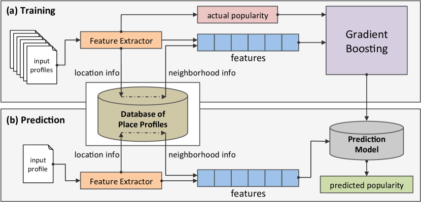
Figure 5: Our location analytics framework.

Figure 6: A break down of the feature vector into six chunks.

4.2 Feature Extraction

The feature extraction module serves to construct a feature vector representing a particular business. In this work, we divide our feature vector into six chunks, which represent different aspects of a target business. Figure 6 summarizes our feature chunks. The first two are associated with categorical data, while the remaining four are about hotspots (i.e., location and “check-ins”) data. Table 2 summarizes the unique identifier (ID), description, and the number of features of each chunk. We describe each chunk below.

Chunk $C_{1}$: The categories of the target business. This chunk is represented using a binary feature vector. For example, a categorical variable with four possible values: “A”, “B”, “C”, and “D” is encoded using four binary features: $[1,0,0,0]$, $[0,1,0,0]$, $[0,0,1,0]$, and $[0,0,0,1]$, respectively. To represent multiple categories, we simply use “0” and “1” to indicate the absence and presence of each category label respectively. For example, we represent a profile with categories “A, C” and another with categories “A, B, C, D” as $[1,0,1,0]$ and $[1,1,1,1]$, respectively. In other words, we use a one-vs-all scheme where we convert multi-class labels to binary labels (i.e., belong or does not belong to the class). As there are a total of 357 unique categories in the dataset of food venues, the binary feature vector will have 357 elements.

Chunk $C_{2}$: The categories of the target business’ neighbors. We first select—from our database of place profiles—the neighboring food businesses within $r$ meters from the target business, after which we extract and sum up the category feature vectors of the neighbors. To define category neighborhood, we use $r=200$ meters, which we found to give optimal performance in our experiments. Similar to $C_{1}$, chunk $C_{2}$ is also a 357-long feature vector that corresponds to the same number of unique categories, except that each feature value is now an integer. Returning to our toy example of the four categories “A”, “B”, “C”, and “D”, if a profile only has 5 neighbors of category “A” and 7 neighbors of category “B”, its integer feature vector will be $[5,7,0,0]$.

Chunks $C_{3}$ and $C_{4}$: Food-related hotspots. The two chunks are related in that both only use food-related neighbors. In other words, they exclude neighbors that have no relevance to food, such as clothing and electronic stores. For each chunk, we are interested in “hotspots”, which are circular areas with the profile in the center and each area is quantified by the “popularity” of stores within it. We define 20 hotspots around the profile whereby each hotspot is demarcated by a maximum distance of $r$ meters, of which $r\in\{50,100,150,\ldots,1000\}$. Finally, the only difference between $C_{3}$ and $C_{4}$ is in how “popularity” is defined; the former computes the (natural) logarithm of the total “check-ins” within a hotspot, while the latter computes the logarithm of the average “check-ins”.

It must be noted that the total and average “check-ins” include only the “check-in” counts of the neighbors and not the count of the target business itself (which is assumed to be unknown). Also, the purpose of applying logarithmic transformation to the “check-in” counts is to reduce the skewness in the counts distribution (i.e., most businesses have small “check-ins” counts, but there is a handful number of businesses with unusually large “check-ins”). In other words, applying logarithm transformation would allow us to mitigate the impact of (unusually) high “check-ins” for popular businesses. Previously, we conducted an experiment that used the raw “check-ins” instead of the logarithmic values. Indeed, we observed that using the logarithm values yielded lower prediction errors than using the raw counts. As such, we shall focus on the results of the logarithm-scaled “check-ins” throughout the rest of this paper.

Chunks $C_{5}$ and $C_{6}$: All (food + non-food) hotspots. These chunks are similar to $C_{3}$ and $C_{4}$, respectively. The only difference is that, instead of solely using food-related neighbors, chunks $C_{5}$ and $C_{6}$ use food and non-food neighbors together. The non-food neighbors include bookshops, transportation facilities like bus and train stations, furniture stores, universities, etc. We include non-food hotspots so as to capture the complementary (non-food) businesses within the neighborhood of a target business.

Table 2: Feature chunks used in our location analytics work.

Chunk ID	Chunk Description	#Features
$C_{1}$	Categories of the profile	357
$C_{2}$	Categories of the profile’s neighbors	357
$C_{3}$	Total “check-ins” of food-related hotspots	20
$C_{4}$	Average “check-ins” of food-related hotspots	20
$C_{5}$	Total “check-ins” of all hotspots	20
$C_{6}$	Average “check-ins” of all hotspots	20

4.3 Predictive Model

In order to learn the association between the extracted features and “check-in” scores of a given business. we train a supervised regression model called gradient boosting machine (GBM) [8]. GBM is a machine learning algorithm that iteratively constructs an ensemble of weak decision tree learners through boosting mechanism. Specifically, the boosting procedure consists of training weak learners and adding them into a final strong model in a forward stage-wise manner. By combining many weak learners that have high bias (i.e., high prediction error), GBM yields an accurate and robust predictive model that has a lower bias than its constituent weak learners [16]. The GBM allows for the optimization of arbitrary differentiable loss functions for classification and/or regression task. For the purpose of “check-in” regression, however, we shall focus on the least square loss function [8] in this work.

Another major benefit of using GBM is that it can automatically derive the so-called feature importance metric [8, 16]. This provides an important mechanism to interpret the trained model and identify the key features that contribute substantially to the prediction of the target variable (i.e., “check-in” score). In particular, each decision tree in the GBM intrinsically performs feature selection by choosing the appropriate split points. This information can then be used to measure the importance of each feature. That is, the more often a feature is used in the split points of a tree, the more important that feature is. This notion can be extended to the tree ensemble by averaging the feature importance of each tree. We further elaborate our feature importance analysis in Section 6.3.

5 Evaluation Preliminaries

We preface our evaluation proper by detailing the evaluation metrics and procedure, the baseline models against which we compare GBM, as well as the model variations we considered in our study.

5.1 Evaluation Metrics and Procedure

To measure how accurate our predicted “check-in” scores differ from the actual (observed) scores, we use two popular regression quality metrics: mean-squared logarithmic error (MSLE) and mean absolute logarithmic error (MALE). The MSLE and MALE metrics are respectively defined as:

$$MSLE =\frac{1}{n}\sum^{n}_{i=1}\left(\log(p_{i}+1)-\log(a_{i}+1)\right)^{2}$$ (1)

$$MALE =\frac{1}{n}\sum^{n}_{i=1}\left|\log(p_{i}+1)-\log(a_{i}+1)\right|$$ (2)

where $n$ is the number of samples in the test set, $p$ is the predicted “check-ins”, and $a$ is the actual “check-ins”. The MSLE metric measures the averaged squared errors, which gives a higher penalty to large logarithmic differences $|\log(p_{i}+1)-\log(a_{i}+1)|$. On the other hand, the MALE metric measures the averaged absolute errors, whereby all the individual differences are weighted equally.

To assess the performance of our predictive model, we perform a 10-fold cross-validation procedure whereby the dataset is randomly partitioned into 10 equal sized subsamples. A single subsample is retained as the validation data for testing our models, while the remaining 9 subsamples are used as training data. The cross-validation process is then repeated 10 times, with each of the 10 subsamples used exactly once as the validation data. We then report the averaged performance.

Finally, to test for the statistical significance of our results, we utilize the independent two-sample t-test [19]. In particular, we look at the $p$-value of the t-test involving two performance vectors, at a significance level of $0.01$. If the $p$-value is less than $0.01$, we can conclude the performance difference is statistically significant.

5.2 Baselines

We compare GBM with several regression baseline algorithms. To foster reproducibility of this work, our implementations of all these algorithms (including GBM) are based on the scikit-learn library [18]. The following baselines are used in this work:

• Distance-based nearest neighbors (DNN). This is a simple baseline that takes the logarithm of the average “check-ins” of the neighbors that reside within some radius $r$ of a target business location. DNN works based on a simple intuition: “the more popular the neighborhood, the more popular the target location is going to be, all else being equal”. We test on $r\in\{50,100,\ldots,500\}$ and found that DNN with $r=100$m brings about the best results.

• Support vector regression with linear kernel (SVR-Linear) [7]. This method produces a linear regression model that depends only on a subset of the training data, since the cost function for building the model ignores any data points close to the model prediction. For this method, we set the cost parameter to $C=1$ and the epsilon parameter (for controlling epsilon-insensitive loss) to $\epsilon=0.1$, which give the best performance in our experiments.

• Support vector regression with radial basis function kernel (SVR-RBF) [23]. This is the same as SVR-Linear, except that now it uses a radial basis function (Gaussian) kernel. As with SVR-Linear, we use $C=1$ and $\epsilon=0.1$, which again constitute the optimal configuration for SVR-RBF.

Last but not least, we configure our GBM algorithm using the “least squares” loss function, a learning rate of 0.1, a maximum tree depth of 10, and a maximum tree width of “sqrt” (i.e., the square root of the total number of features). For the number of boosting iterations $N$, we perform an exhaustive grid search on $N\in\{100,200,\ldots,5000\}$ and found that $N=1000$ produces the best results. Note that, in each boosting iteration, a new tree is created and added into the ensemble. As such, the number of boosting iterations $N$ is equal to the number of trees constructed.

5.3 Model Variations

To evaluate the contributions of different feature chunks, we construct a variation of the predictive models by enumerating all possible combinations of the six chunks (see Section 4.2). That is, we construct all possible $2^{6}-1=63$ chunk combinations and build a predictive model for each combination. We represent a model variant using a binary array of length six, where chunk $C_{i}$ maps to the $i^{th}$ element in the array. We use the notation “$\text{[model\_name]}_{\text{xxxxxx}}$” to represent a particular model variant, where $\text{x}\in\{0,1\}$. For example, a GBM model using $C_{1}$, $C_{2}$, and $C_{4}$ is denoted as $\text{GBM}_{\text{110100}}$. Note that DNN does not use this notation, since it works based on spatial distance only, instead of feature chunks. For SVR-Linear, SVR-RBF and GBM, we run experiments on all 63 variants and report the best results for each of the three methods.

6 Results and Analysis

We now present our main experimental results. Our experiments seek to answer several key research questions (RQs):

RQ1:

How well can our predictive model (GBM) estimate the popularity (i.e., “check-in” scores) of business locations?

RQ2:

What are the contributions of different feature chunks? How robust is our model against different feature combinations?

RQ3:

Do the important features found by our model make sense? What can we learn/conclude from them?

6.1 Performance Assessment (RQ1)

Table 3 compares the cross-validation performances (i.e., averaged MALE and MSLE) of different regression methods. For SVR-Linear and SVR-RBF, we show both the “full variant” (i.e., $\text{SVR-Linear}_{\text{111111}}$ and $\text{SVR-RBF}_{\text{111111}}$) as well as the variants that give the best results for the same method (i.e., $\text{SVR-Linear}_{\text{111000}}$ and $\text{SVR-RBF}_{\text{100011}}$). We observe that GBM consistently and significantly outperforms other models (at $p<0.01$), particularly against $\text{SVR-RBF}_{\text{100011}}$, which is the best among all the baselines.

Table 3: Performance comparisons of different models.

Model	Feature Chunks	MALE	MSLE
DNNr=100m	-	1.99305	7.27499
SVR-Linear111000	$\{C_{1},C_{2}\}$	1.59072	4.25301
SVR-Linear111111	$\{C_{1},C_{2},C_{3},C_{4},C_{5},C_{6}\}$	2.12345	7.35446
SVR-RBF100011	$\{C_{1},C_{5},C_{6}\}$	1.47518	3.61863
SVR-RBF111111	$\{C_{1},C_{2},C_{3},C_{4},C_{5},C_{6}\}$	1.53067	3.92219
GBM111111	$\{C_{1},C_{2},C_{3},C_{4},C_{5},C_{6}\}$	1.16362*	2.56924*
*: significant at 0.01 with respect to SVR-RBF100011

We can explain the results in terms of model complexity. For instance, we can expect the simplest nearest neighbor method (i.e., DNN) to be beaten by other methods, as it only uses spatial distance. We can also anticipate that SVR-RBF would outperform SVR-Linear, as the RBF kernel maps the original features into a high-dimensional space. This expanded feature space provides SVR-RBF with a greater representation power to model a much more complex relationship than SVR-Linear. Finally, as GBM combines weak learners into a strong learner, the aggregate prediction of the ensemble is more accurate than the prediction of any of its constituent learners. This aggregation also provides GBM with more robustness to data overfitting, as compared to SVM-RBF.

Additionally, the results in Table 3 suggest that the two SVR methods are more sensitive to the variation of feature chunks, particularly to the presence of less relevant (or irrelevant) features. This can be attributed to the fact that each tree in GBM intrinsically performs feature selection, for which less important features are unlikely to be chosen and used in the ensemble. Indeed, we can see that SVR-Linear with all six chunks (i.e., $\text{SVR-Linear}_{\text{111111}}$) is outperformed by the simpler SVR-Linear variant (i.e., $\text{SVR-Linear}_{\text{111000}}$) that uses only three chunks. Surprisingly, the former is also outperformed by even the DNN method. The same conclusion can be made by comparing $\text{SVR-RBF}_{\text{111111}}$ and $\text{SVR-RBF}_{\text{100011}}$. On the contrary, GBM is more robust against inconsequential features. In fact, GBM generally improves its performance as we add more chunks, as we will see shortly in Section 6.2.

6.2 Contribution of Feature Chunks (RQ2)

The partitioning of the feature vectors into six chunks allows us to investigate the contribution of each feature group. Table 4(a) lists the top $10$ GBM variants (out of $63$ possible variants), sorted in an ascending order of their MALE scores. Similarly, Table 4(b) lists the top 10 GBM variants, sorted in ascending order of their MSLE scores. Note that the top $10$ GBM variants happen to be the same for the two tables, except that they have slightly different ordering. From the results, it is evident that $\text{GBM}_{\text{111111}}$ does not significantly outperform the other nine variants (at a significance level of $0.01$). This shows that GBM is robust against the variation of feature chunks. We can also see that the performance of the GBM improves as we add more feature chunks. Again, this can be attributed to the feature selection mechanism of each tree in the ensemble, which helps exclude irrelevant features.

Table 4: Cross-validation results of the top 10 GBM variants.

(a) MALE results of the top 10 GBM variants.

	Feature Chunks
Model	$C_{1}$	$C_{2}$	$C_{3}$	$C_{4}$	$C_{5}$	$C_{6}$	MALE
GBM111111	Yes	Yes	Yes	Yes	Yes	Yes	1.163618
GBM111100	Yes	Yes	Yes	Yes	–	–	1.172693
GBM111010	Yes	Yes	Yes	–	Yes	–	1.173910
GBM110011	Yes	Yes	–	–	Yes	Yes	1.175062
GBM101111	Yes	–	Yes	Yes	Yes	Yes	1.177136
GBM101100	Yes	–	Yes	Yes	–	–	1.182053
GBM100011	Yes	–	–	–	Yes	Yes	1.184053
GBM111000	Yes	Yes	Yes	–	–	–	1.184895
GBM110010	Yes	Yes	–	–	Yes	–	1.189258
GBM101010	Yes	–	Yes	–	Yes	–	1.191831
Count	10	6	7	4	7	4

(b) MSLE results of the top 10 GBM variants.

	Feature Chunks
Model	$C_{1}$	$C_{2}$	$C_{3}$	$C_{4}$	$C_{5}$	$C_{6}$	MSLE
GBM111111	Yes	Yes	Yes	Yes	Yes	Yes	2.569236
GBM111010	Yes	Yes	Yes	–	Yes	–	2.608927
GBM101111	Yes	–	Yes	Yes	Yes	Yes	2.609254
GBM111100	Yes	Yes	Yes	Yes	–	–	2.610255
GBM110011	Yes	Yes	–	–	Yes	Yes	2.615818
GBM101100	Yes	–	Yes	Yes	–	–	2.627101
GBM100011	Yes	–	–	–	Yes	Yes	2.628505
GBM111000	Yes	Yes	Yes	–	–	–	2.653032
GBM110010	Yes	Yes	–	–	Yes	–	2.660369
GBM101010	Yes	–	Yes	–	Yes	–	2.667292
Count	10	6	7	4	7	4

Based on the binary representation of the six chunks, we can also calculate the relative significance of a chunk by counting the number of times in which it is present (i.e., when the chunk is assigned the value of $1$). The sum of each chunk’s presence in the $10$ GBM variants is shown at the last row of Tables 4(a) and 4(b), entitled “Count”. We see that the categories of the target business (i.e., chunk $C_{1}$) is present in all the top 10 GBM variants, indicating that it is an essential feature. This may seem to suggest that the nature of the business itself plays a pivotal role. However, as described in Section 3.2, food businesses on Facebook may contain non-food labels such as “airport” and “shopping mall” (e.g., for a cafe located in the shopping mall of an airport). In turn, this suggests that the “environment” around a selected business is also a key factor. The method of chunk counting presented in this section is a coarse-grained analysis and is not sufficient to validate this conjecture. We will further analyze this in Section 6.3, where we employ a more fine-grained analysis of the individual feature’s importance.

Moving on, we also notice that the total “check-ins” chunks (i.e., chunks $C_{3}$ and $C_{5}$) are ranked higher than the average “check-ins” (i.e., $C_{4}$ and $C_{6}$), i.e., the counts are 7/10 vs. 4/10. This suggests that the total “check-ins” have more discriminatory power than the average “check-ins”, which could be due to the averaging failing to account for the number of business nearby. On the other hand, total “check-ins” (of an area) gives a more accurate reflection of the potential human traffic that an area has. Finally, we see no substantial performance difference between food-related hotspots and all (i.e., food + non-food) hotspots (both have a count sum of $7+4=11$). This implies that the presence of non-food-related categories does not contribute significantly to the prediction quality.

6.3 Analysis of Feature Importance (RQ3)

The analysis of the six chunks of the feature vectors in the previous section represents a coarse-grained analysis. To perform a more fine-grained analysis, we look into the full feature vector (with all six chunks included) in the $\text{GBM}_{\text{111111}}$ model and try to compute the relative importance of each individual feature. GBM derives this automatically, by measuring how many times a feature is used in the split points of a tree [8] (see also Section 4.3).

Figure 7(a) shows the relative importance of the top 20 features in descending order of importance, while Figure 7(b) shows the relative importance of the $71^{st}$ to the $90^{th}$ features. (We do not include the results for the $21^{st}$ to $70^{th}$ features here, as the changes in the feature importance score are fairly smooth.) Accordingly, we can make the following observations:

• Chunks $C_{3}$ to $C_{6}$ (black bars in Figure 7) dominate the top 80 feature importance positions (not fully shown in Figure 7), and it is not until the $\text{81}^{\text{st}}$ top feature that chunks $C_{1}$ and $C_{2}$ show up. This suggests that hotspot features play a very crucial role: the more “check-ins” a target business’ neighbors have, the more popular the target business is likely to be.

• From Figure 7(a), 14 out of 20 hotspot features are below 500m, suggesting that nearer “check-ins” are used as a strong signal to make a split in the decision tree. This is not surprising, as it may be physically tiring for customers to travel farther than 500m, and most will settle all their outdoor needs in a specific area, such as a shopping mall.

• Comparing the total and average “check-ins” in Figure 7(a), 14 out of 20 features belong to the former. This indicates that total “check-ins” is a better input feature/signal for split points in the GBM’s trees. This finding is generally in agreement with what we have found in Section 6.2.

• Figure 7(a) also shows that the type of neighbors (i.e., “food-only” or “all”) are equally matched with 10 counts each. Again, this finding conforms with the earlier finding in Section 6.2. Note that, despite the different approaches in Sections 6.2 and 6.3, both arrived at the similar conclusion with regard to the type of “check-in” and the type of neighbor.

• From the colored bars (i.e., chunks $C_{1}$ and $C_{2}$) in Figure 7(b), we see that $C_{1}$ is dominated by the $C_{2}$. This suggests that categories of the neighboring businesses are more important than those of the target business ($C_{1}$). Together with the “hotspot” features in Chunks $C_{3}$ to $C_{6}$, this reinforces the idea of a “local effect” whereby business benefit by being close to more established neighbors.

• Finally, we notice a significant and faster drop in the importance scores from the $\text{81}^{\text{st}}$ to $\text{90}^{\text{th}}$ features (as compared from the $1^{st}$ to $80^{th}$). In this case, places or franchises that typically attract general (and larger) crowd, such as “restaurant”, “coffee”, or “shopping mall”-related categories, take the first top spots among the neighbors’ categories. This suggests that food-related categories (of the neighbors) are more important than the non-food categories.

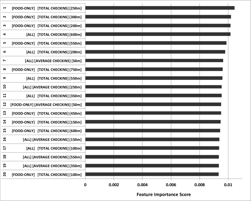
(a) Feature importance of the top 20 features descending order
of importance. The top 20 happen to consists of Chunks $C_{3}$ to $C_{6}$.

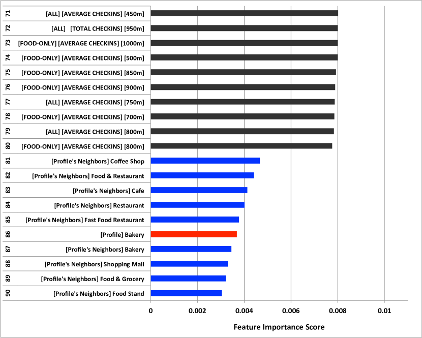
(b) Feature importance of the top $\text{71}^{\text{st}}$ to $\text{90}^{\text{th}}$ features. Besides Chunks $C_{3}$ to $C_{6}$, it also contains Chunks $C_{1}$ and $C_{2}$, in red and blue, respectively.

Figure 7: Top features from the feature importance of the $\text{GBM}_{\text{111111}}$ model.

7 Web Application Prototype

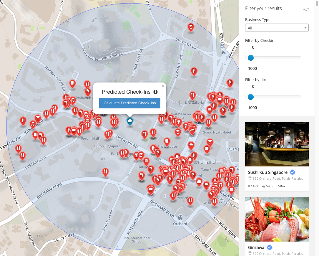
Figure 8: Our online interactive location analytics system.

We implement our location analytics framework as an interactive web application service, which can be accessed at: https://research.larc.smu.edu.sg/bizanalytics/.

Technologies. We employ the following technologies to build our web application: (i) Python (implementing the predictive model and feature extraction), (ii) RabbitMQ (a messaging passing system that allows querying the predictive model), (iii) Node.js (for processing users’ queries and returning the prediction results to the front-end), (iv) ElasticSearch (a distributed search engine for quering the database of place profiles), and (v) Google Maps (for visualization at the front-end). This configuration provides an efficient and scalable way to process a user’s location query (via Node.js and RabbitMQ), retrieve the relevant neighbors (via ElasticSearch), involve feature extraction and predictive models (in the Python component), and finally display the prediction results to the users (again via Node.js and RabbitMQ, along with Google Maps).

User interaction. Figure 8 shows an example of how our web application works. A user drops a pin (i.e., the blue pin in the middle of the screen) to indicate where his (hypothetical) store location would be. Depending on the location, the interface also dynamically shows the neighboring businesses on the right panel and their respective information, such as (i) the distance from the drop-pin, and (ii) the number of physical “check-ins” and “likes”. When the user is ready, he/she may click the “Calculate Predicted Check-ins” button, which will then calculate the predicted “check-in” score on the fly. After presenting the predicted “check-in” score, the user can also open a new panel, showing a ranked list of his/her target location relative to the nearby businesses (Figure 9). The ranking allows users to understand how their target location would fare against the neighboring businesses. The panel also shows the highest, lowest, and the median scores of these neighbors.

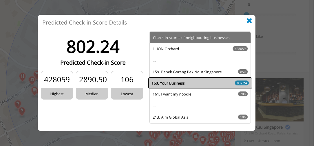
Figure 9: After computing the predicted “check-in” score, users can compare their target location with the surrounding businesses.

Qualitative study. Figures 8 and 9 demonstrate the on-the-fly prediction of our web application, where it is able to predict the “check-in” score of a hypothetical, inexistent target business. For this example, the score of $802.24$ in Figure 9 represents a fairly conservative prediction of the potential “check-ins” in the target location (i.e., the blue pin) and the selected type of business. This hypothetical business is ranked $160^{th}$ among $213$ businesses, with the lowest “check-ins” being $106$. This is a reasonable prediction. On the one hand, because the place is near places with consistent human traffic, such as the Hilton Hotel and several other shopping malls, it should garner a decent amount of check-ins. On the other hand, as there are many other businesses in the area (the area is a renowned shopping paradise in Singapore), it may be challenging for the hypothetical business to compete with these businesses.

8 Discussion and Future Work

In this work, we investigate whether businesses can benefit from other (popular) businesses within its vicinity. Our results show not only a positive correlation between the popularity of a target business and its neighbors, but also the critical importance of the “hotspot” features: the nearer a target location is to a popular place with larger “check-ins”, the more successful it would be. This finding conforms with our intuition. But more importantly, it demonstrates that ubiquitous online data (such as Facebook Pages) can be used to gauge the socioeconomical values. We also show how our predictive model can be used to accurately estimate the “check-in” score of a particular location, allowing us to identify the best locations that would bring popularity, and by extension, success.

Despite the promising potentials of our approach, there remains room for improvement. For instance, our current work has not taken into account the temporal aspects of the business popularity, such as modeling the trend of the “check-in” scores over time. Further quantitative and qualitative studies may also be needed in the future to compare our work with other location-based services such as Foursquare. To facilitate more comprehensive location analytics, we can extend our approach by building a two-level location recommendation system, whereby we first (coarsely) recommend a city district [15] and then pinpoint (multiple) promising locations within that district. As we include more data, such as non-food categories and auxiliary data that reflect the human flow of different areas of an urban city, we will be able to further improve on our current model and findings. To address all these, we plan to develop a new spatiotemporal predictive model that integrates a richer set of residential, demographics, and other social media data.

Acknowledgements. This research is supported by the National Research Foundation, Prime Minister’s Office, Singapore under its International Research Centres in Singapore Funding Initiative.

References

- [1] J. Chang and E. Sun. Location3: How users share and respond to location-based data on social networking sites. In Proceedings of the International AAAI Conference on Weblogs and Social Media, pages 74–80, 2011.
- [2] H. Chen, R. H. L. Chiang, and V. C. Storey. Business intelligence and analytics: From big data to big impact. MIS Quarterly, 36(4):1165–1188, 2012.
- [3] N. Cohen. Business location decision-making and the cities: Bringing companies back. Technical report, Brookings Institution Center on Urban and Metropolitan Policy, 2000.
- [4] ESRI. Revealing the “where” of business intelligence using location analytics. http://www.esri.com/library/whitepapers/pdfs/business-intelligence-location-analytics.pdf, 2012.
- [5] Facebook. Facebook platform upgrade guide. https://developers.facebook.com/docs/apps/upgrading, 2016.
- [6] Facebook. Graph API reference. https://developers.facebook.com/docs/graph-api/reference/page, 2016.
- [7] R.-E. Fan, K.-W. Chang, C.-J. Hsieh, X.-R. Wang, and C.-J. Lin. LIBLINEAR: A library for large linear classification. Journal of Maching Learning Research, 9:1871–1874, 2008.
- [8] J. H. Friedman. Greedy Function Approximation: A Gradient Boosting Machine. The Annals of Statistics, 29:1189–1232, 2001.
- [9] H. Gao, J. Tang, X. Hu, and H. Liu. Exploring temporal effects for location recommendation on location-based social networks. In Proceedings of the ACM Conference on Recommender Systems, pages 93–100, 2013.
- [10] H. Gao, J. Tang, X. Hu, and H. Liu. Modeling temporal effects of human mobile behavior on location-based social networks. In Proceedings of the ACM Conference on Information and Knowledge Management, pages 1673–1678, 2013.
- [11] L. Garber. Analytics goes on location with new approaches. IEEE Computer, 46(4):14–17, 2013.
- [12] P. Georgiev, A. Noulas, and C. Mascolo. Where businesses thrive: Predicting the impact of the Olympic Games on local retailers through location-based services data. In Proceedings of the International AAAI Conference on Weblogs and Social Media, pages 151–160, 2014.
- [13] D. Karamshuk, A. Noulas, S. Scellato, V. Nicosia, and C. Mascolo. Geo-spotting: Mining online location-based services for optimal retail store placement. In Proceedings of the ACM SIGKDD International Conference on Knowledge Discovery and Data Mining, pages 793–801, 2013.
- [14] R. Li, S. Wang, and K. C.-C. Chang. Multiple location profiling for users and relationships from social network and content. Proceedings of the International Conference on Very Large Data Bases, 5(11):1603–1614, 2012.
- [15] J. Lin, R. J. Oentaryo, E.-P. Lim, C. Vu, A. Vu, A. T. Kwee, and P. K. Prasetyo. A business zone recommender system based on Facebook and urban planning data. In Proceedings of the European Conference on Information Retrieval, pages 1–7, 2016.
- [16] A. Natekin and A. Knoll. Gradient boosting machines: A tutorial. Frontiers in Neurorobotics, 7(21):1–21, 2013.
- [17] A. Noulas, S. Scellato, N. Lathia, and C. Mascolo. Mining user mobility features for next place prediction in location-based services. In Proceedings of the IEEE International Conference on Data Mining (ICDM), pages 1038–1043, 2012.
- [18] F. Pedregosa, G. Varoquaux, A. Gramfort, V. Michel, B. Thirion, O. Grisel, M. Blondel, P. Prettenhofer, R. Weiss, V. Dubourg, J. Vanderplas, A. Passos, D. Cournapeau, M. Brucher, M. Perrot, and E. Duchesnay. Scikit-learn: Machine learning in python. Journal of Machine Learning Research, 12:2825–2830, 2011.
- [19] W. H. Press, B. P. Flannery, S. A. Teukolsky, and W. T. Vetterling. Numerical Recipes in C: The Art of Scientific Computing. Cambridge University Press, 1988.
- [20] R. W. Sinnott. Virtues of the haversine. Sky and Telescope, 68(2):159, 1984.
- [21] C. Smith. 200+ amazing facebook user statistics. http://expandedramblings.com/index.php/by-the-numbers-17-amazing-facebook-stats/, 2016.
- [22] C. Smith. By the numbers: 17 important Foursquare stats. http://expandedramblings.com/index.php/by-the-numbers-interesting-foursquare-user-stats/, 2016.
- [23] A. J. Smola and B. Schölkopf. A tutorial on support vector regression. Statistics and Computing, 14(3):199–222, 2004.
- [24] B. Thau. How big data helps chains like starbucks pick store locations—an (unsung) key to retail success. http://onforb.es/1iijr2o, 2015.
- [25] Y. Zhang, B. Li, and J. Hong. Understanding user economic behavior in the city using large-scale geotagged and crowdsourced data. In Proceedings of the International World Wide Web Conference, 2016.