A Cut Finite Element Method for the Bernoulli Free Boundary Value Problem

Abstract

We develop a cut finite element method for the Bernoulli free boundary problem. The free boundary, represented by an approximate signed distance function on a fixed background mesh, is allowed to intersect elements in an arbitrary fashion. This leads to so called cut elements in the vicinity of the boundary. To obtain a stable method, stabilization terms is added in the vicinity of the cut elements penalizing the gradient jumps across element sides. The stabilization also ensures good conditioning of the resulting discrete system. We develop a method for shape optimization based on moving the distance function along a velocity field which is computed as the $H^{1}$ Riesz representation of the shape derivative. We show that the velocity field is the solution to an interface problem and we prove an a priori error estimate of optimal order, given the limited regularity of the velocity field across the interface, for the the velocity field in the $H^{1}$ norm. Finally, we present illustrating numerical results.

Keywords. Free boundary value problem; CutFEM; Shape optimization; Level set; Fictitious domain method

1 Introduction

In this paper we consider the application of the recently developed cut finite element method (CutFEM) [4, 6] to the Bernoulli free boundary problem. This problem appears in a variety of applications such as stationary water waves (Stokes waves) and the optimal insulation problem. The Bernoulli free boundary problem is very well understood from the mathematical point of view, see [3, 14, 26] and the references therein, and it also serves as a standard test problem for different optimization and numerical methods, see e.g. [18, 21, 22] among others. When numerically solving free boundary problems it is highly beneficial to avoid updating the computational mesh when updating the boundary, since large motions of the boundary may require complete remeshing. This can be achieved by the use of fictitious domain methods, which, however, are known not to perform very well for shape optimization or free surface problems due to their lack of accuracy close to the boundary [17]. An exception is the least squares formulation suggested in [13], where similarly as in [6] the formulation is restricted to the physical domain.

A fictitious domain method which does not lose accuracy close to the boundary is the recently developed CutFEM method, see [4]. CutFEM uses weak enforcement of the boundary conditions and a sufficiently accurate representation of the domain together with certain consistent stabilization terms to guarantee stability, optimal accuracy, and conditioning independent of the position of the boundary in the background mesh. Furthermore, no expensive and complicated mesh operations (edge split, edge collapse, remeshing, etc.) need to be performed when updating the boundary. This is a significant gain especially for complicated boundaries and for 3D applications. CutFEM has successfully been applied for problems with unknown or moving boundaries in, e.g., [8, 16].

As in [1, 2] we consider a shape optimization approach to solve the Bernoulli free boundary problem using sensitivity analysis and a level set representation [24] to track the evolution of the free boundary. In the sensitivity analysis we do not use the standard Hadamard structure of the shape functional, i.e., we do not express the shape functional as a normal perturbation of the boundary. Instead we use a volume representation which requires less smoothness and has proved to possess certain superconvergence properties compared to the boundary formulation [20], see also [19, 23]. To obtain a velocity field from the shape derivate, we use the Hilbertian regularization suggested in [12], where we essentially let the velocity field on the domain be defined as the solution to the weak elliptic problem associated with the $H^{1}$ inner product with right hand side given by the shape derivative functional. We may thus view the velocity field as the $H^{1}$ Riesz representation of the shape derivative functional acting on $H^{1}$. This procedure leads to an elliptic interface problem for the velocity field. The free boundary is then updated by moving the level set along the velocity field.

We derive a priori error estimates for the CutFEM approximation of the primal problem and the dual problem, involved in the computation of the shape derivative in the $W^{1}_{p}$, $2\leq p<\infty$, norm, and then we use these estimates to prove an a priori error estimate for the discrete approximation of the velocity field in the $H^{1}$ norm. In the error estimates for the primal and dual problems we use inverse estimates, for $2<p<\infty$, which leads to suboptimal convergence rates, but it turns out these bounds are indeed sharp enough to prove optimal order estimates for the discrete velocity field.

An outline of the paper is as follows: in Section 2 we present the model problem and CutFEM discretization, in Section 3 we use sensitivity analysis to derive the shape derivative, in Section 4 we discuss how to compute a regularized descent direction from the shape derivative, in Section 5 we present a level set representation of the free boundary and method for computing its evolution, in Section 6 we present an optimization algorithm, in Section 7 we present a priori error estimates of the CutFEM approximation of the primal and dual problems as well as for the discrete approximation of the velocity field, and finally, in Section 8 we present numerical experiments to verify the convergence rates and overall behavior of the optimization algorithm.

2 Model Problem and Finite Element Method

2.1 Model Problem

We consider the Bernoulli free boundary value problem:

$$-\Delta u =f \text{in }\Omega$$ (2.1)

$$u =g_{D} \text{on }\partial\Omega$$ (2.2)

$$n\cdot\nabla u =g_{N} \text{on }\Gamma$$ (2.3)

where $\Gamma\subset\partial\Omega$ is the free and $\partial\Omega\setminus\Gamma$ is the fixed part of the boundary, $g_{D}=0$ and $g_{N}$ is constant on $\Gamma$. Note the double boundary conditions on $\Gamma$. We seek to determine the domain $\Omega$ such that there exist a solution $u$ to (2.1)-(2.3). For $f=0$ we refer to [3, 14, 26] and the references therein for theoretical background of the Bernoulli free boundary value problem and for $f=0$ we assume that $f$ is such that there exist a unique solution.

In order to obtain a formulation which is suitable as a starting point for a numerical algorithm we recast the overdetermined boundary value problem as a constrained minimization problem as follows. We seek to minimize the functional

$$J(\Omega):=J(\Omega;u(\Omega))=\min_{\Omega}\frac{1}{2}\int_{\Gamma}u^{2}\,\text{\rm d}\Gamma$$ (2.4)

where the function $u$ solves the boundary value problem

$$-\Delta u =f \text{in }\Omega$$ (2.5)

$$u =g_{D} \text{on }\Gamma_{\rm{fix}}:=\partial\Omega\setminus\Gamma$$ (2.6)

$$n\cdot\nabla u =g_{N} \text{on }\Gamma$$ (2.7)

Note that we keep the Neumann condition on the free boundary and enforce the Dirichlet condition through the minimization of the functional $J(\Omega)$.

The weak formulation of (2.5-2.7) reads: find $u\in V_{g_{D}}(\Omega):=\{v\in H^{1}(\Omega):v|_{\Gamma_{\mathrm{fix}}}=g_{D}\}$ such that

$$a(\Omega;u,v):=\int_{\Omega}\nabla u\cdot\nabla v\,\text{\rm d}\Omega=\int_{\Omega}f\,\text{\rm d}\Omega=:F(\Omega;v)\qquad\forall v\in V_{0}(\Omega)$$ (2.8)

Let $\mathcal{O}$ be the set of admissible domains; then the constrained minimization problem reads: find $\Omega\in\mathcal{O}$ such that

$$J(\Omega) =\min_{\Omega\in\mathcal{O}}J(\Omega;v)\quad$$ (2.9)

$$\text{for }u\in V_{g_{D}}(\Omega)\text{ s.t. } a(\Omega;u,v)=F(\Omega;v)\quad\forall v\in V_{0}(\Omega)$$ (2.10)

To solve the minimization problem (2.9)-(2.10), we define the corresponding Lagrangian as

$$\mathcal{L}(\omega,v,q):=J(\omega;u)-a(\omega;v,q)+F(\omega;q)$$ (2.11)

That is, we seek the domain $\Omega$ such that

$$\Omega=\operatorname*{arg\,min}\{\omega\in\mathcal{O}\mid\min_{v\in V_{g_{D}}(\omega)}\max_{q\in V_{0}(\omega)}\mathcal{L}(\omega,v,q)\}$$ (2.12)

2.2 Cut Finite Element Method

We will use a cut finite element method to discretize the boundary value problem (2.8). Before formulating the method we introduce some notation.

The Mesh and Finite Element Space.

Let $\Omega_{0}$ be a polygonal domain such that all admissible domains $\Omega\in\mathcal{O}$ are subsets of $\Omega_{0}$, i.e. $\Omega\subset\Omega_{0}$. Let $\mathcal{T}_{h,0}$ denote a family of quasiuniform triangulations of $\Omega_{0}$ with mesh parameter $h\in(0,h_{0}]$ and define the corresponding space of continuous piecewise linear polynomials

$$V_{h}(\Omega_{0})=\{v\in H^{1}(\Omega_{0}):v|_{T}\in P_{1}(T),\quad\forall T\in\mathcal{T}_{h,0}\}$$ (2.13)

Given $\Omega\in\mathcal{O}$ we define the active mesh

$${\mathcal{T}_{h}}=\{T\in\mathcal{T}_{h,0}:\overline{T}\cap\overline{\Omega}\neq\emptyset\}$$ (2.14)

the union of the active elements

$$\Omega_{h}=\cup_{T\in{\mathcal{T}_{h}}}T$$ (2.15)

and the finite element space on the active mesh

$$V_{h}(\Omega)=V_{h}(\Omega_{0})|_{\Omega_{h}}$$ (2.16)

Let also $\mathcal{F}_{h}$ denote the set of interior faces in ${\mathcal{T}_{h}}$ such that at least one of its neighboring elements intersect the boundary $\partial\Omega$,

$${\mathcal{F}_{h}}=\{F:T^{+}_{F}\cap\partial\Omega\neq\emptyset\text{ or }T^{-}_{F}\cap\partial\Omega\neq\emptyset\}$$ (2.17)

where, $T^{+}_{F}$ and $T^{-}_{F}$ are the two elements sharing the face $F$. On a face $F$ we define the jump

$$\llbracket v\rrbracket=v|_{T^{+}_{F}}-v|_{T^{-}_{F}}$$ (2.18)

where $T^{+}_{F}$ is the element with the higher index.

The Method.

We define the forms

$$A_{h}(\Omega;v,w) =a_{h}(\Omega;v,w)+s_{h}(v,w)$$ (2.19)

$$a_{h}(\Omega;v,w) =(\nabla v,\nabla w)_{\Omega}-(\partial_{n}v,w)_{\Gamma_{\rm{fix}}}-(\partial_{n}w,v)_{\Gamma_{\rm{fix}}}+(\gamma_{D}h^{-1}v,w)_{\Gamma_{\rm{fix}}}$$

$$s_{h}(\Omega;v,w) =\sum_{F\in{\mathcal{F}_{h}}}(\gamma_{1}h\llbracket\partial_{n}v\rrbracket,\llbracket\partial_{n}w\rrbracket)_{F}$$ (2.20)

$$F_{h}(\Omega;w) =(f,w)_{\Omega}+(g_{D},\gamma_{D}h^{-1}w-\partial_{n}w)_{\Gamma_{\rm{fix}}}+(g_{N},w)_{\Gamma}$$ (2.21)

were $(u,v)_{\omega}:=\int_{\omega}u\cdot v\,\text{d}\omega$ is the $L^{2}$ inner product over the set $\omega$ equipped with the appropriate measure. Our method for the approximation of (2.5)–(2.7) takes the form: find $u_{h}\in V_{h}(\Omega)$ such that

$$A_{h}(\Omega;u_{h},v)=F_{h}(\Omega;v)\quad\forall v\in V_{h}(\Omega)$$ (2.22)

We recognize the weak enforcement of Dirichlet boundary conditions by Nitsche’s method, cf. [15]. Furthermore, the term $s_{h}$, first suggested in this context in [6], is added to stabilize the method in the vicinity of the boundary.

3 Shape Derivative

3.1 Definition of the Shape Derivative

For $O\in\mathcal{O}$ we let $W(\Omega,\mathbb{R}^{d})$ denote the space of sufficiently smooth vector fields and for a vector field $\vartheta\in W$ we define the map

$$\mathcal{M}_{\vartheta}:\Omega\times I\ni(x,t)\mapsto x+t\vartheta(x)\in\mathcal{M}_{\vartheta}(\Omega,t)\subset\mathbb{R}^{d}$$ (3.1)

where $I=(-\delta,\delta)$, $\delta>0$. For small enough $\delta$, the mapping $\Omega\mapsto\mathcal{M}_{\vartheta}(\Omega,t)$ is a bijection and $\mathcal{M}_{\vartheta}(\Omega,0)=\Omega$. We also assume that the vector field $\vartheta$ is such that $\mathcal{M}_{\vartheta}(\Omega,t)\in\mathcal{O}$ for $t\in I$ with $\delta$ small enough.

Let $J(\Omega)$ be a shape functional, i.e., a mapping $J:\mathcal{O}\ni\Omega\mapsto J(\Omega)\in\mathbb{R}$. We then have the composition $I\ni t\mapsto J\circ\mathcal{M}(\Omega,t)\in\mathbb{R}$ and we define the shape derivative $D_{\Omega,\vartheta}$ of $J$ in the direction $\vartheta$ by

$$D_{\Omega,\vartheta}J(\Omega)=\frac{d}{dt}J\circ\mathcal{M}_{\vartheta}(\Omega,t)|_{t=0}=\lim_{t\to 0}\frac{J(\mathcal{M}_{\vartheta}(\Omega,t))-J(\Omega)}{t}$$ (3.2)

Note that if $\mathcal{M}_{\vartheta}(\Omega,t)=\Omega$ we have $D_{\Omega,\vartheta}J=0$, even if $\mathcal{M}_{\vartheta}$ change points in the interior of the domain.

We finally define the shape derivative $D_{\Omega}J|_{\Omega}:W(\Omega,\mathbb{R}^{d})\rightarrow\mathbb{R}$ by

$$D_{\Omega}J|_{\Omega}(\vartheta)=D_{\Omega,\vartheta}J(\Omega)$$ (3.3)

In cases when the functional $J$ depend on other arguments we use $\partial_{\Omega}$ to denote the partial derivative with respect to $\Omega$ and $\partial_{\Omega,\vartheta}$ to denote the partial derivative with respect to $\Omega$ in the direction $\vartheta$.

3.2 Leibniz Formulas

For $v:\Omega\times I\rightarrow\mathbb{R}^{d}$ we define the material time derivative in the direction $\vartheta$ by

$$D_{t,\vartheta}v=\lim_{t\to 0}\frac{v(\mathcal{M}_{\vartheta}(x,t),t)-v(x,0)}{t}$$ (3.4)

and the partial time derivative by

$$\partial_{t}v=\lim_{t\to 0}\frac{v(x,t)-v(x,0)}{t}$$ (3.5)

From the chain rule it follows that

$$D_{t,\vartheta}v=\partial_{t}v+\vartheta\cdot\nabla v$$ (3.6)

The material derivative does not commute with the gradient and we have the commutator

$$[D_{t,\vartheta},\nabla]v=D_{t,\vartheta}(\nabla v)-\nabla(D_{t,\vartheta}v)=-(D\vartheta)^{T}\nabla v$$ (3.7)

where $D\vartheta=V\otimes\nabla$ is the derivative (or Jacobian) of the vector field $\vartheta$, and the usual product rule

$$D_{t,\vartheta}{(vw)}=(D_{t,\vartheta}v)w+v(D_{t,\vartheta}w)$$ (3.8)

holds. To derive a expression of the shape derivative, the following lemma will be used frequently.

Lemma 3.1.

Let $f,g:\mathbb{R}^{d}\to\mathbb{R}$ be functions smooth enough for the following expressions to be well defined. Then the following relationships hold

$$D_{\Omega,\vartheta}\int_{\Omega}f\,\text{\rm d}\Omega =\int_{\Omega}\left(D_{t,\vartheta}f+(\nabla\cdot\vartheta)f\right)\,\text{\rm d}\Omega$$ (3.9)

$$D_{\Omega,\vartheta}\int_{\Gamma}g\,\text{\rm d}\Gamma =\int_{\Gamma}\left(D_{t,\vartheta}g+(\nabla_{\Gamma}\cdot\vartheta)g\right)\,\text{\rm d}\Gamma$$ (3.10)

where $\nabla_{\Gamma}\cdot v=\nabla\cdot v-n\cdot D\vartheta\cdot n$ and $n$ is the unit normal to $\Gamma$.

Proof.

The proof can e.g. be found in [27]. ∎

Remark 3.1.

An alternative definition of the surface divergence is $\nabla_{\Gamma}\cdot\vartheta=\text{tr}(\vartheta\otimes\nabla_{\Gamma})$ where $\nabla_{\Gamma}v=(1-n\otimes n)\nabla v$ is the tangent gradient.

3.3 Shape Derivative of the Lagrangian formulation

Recall the Lagrangian

$$\mathcal{L}(\omega,v,q)=J(\omega;v)-a(\omega;v,q)+F(\omega;q)$$ (3.11)

For a fixed $\Omega\in\mathcal{O}$ we take the Fréchet derivative $D\mathcal{L}(\Omega,\cdot,\cdot):V_{0}(\Omega)\times V_{0}(\Omega)\rightarrow\mathbb{R}$ of $\mathcal{L}$,

$$D\mathcal{L}|_{(\Omega,u,p)}(\delta u,\delta p)=\left\langle D\mathcal{L}|_{(\Omega,u,p)},\left(\delta u,\delta p\right)\right\rangle=\underbrace{\left\langle\partial_{v}\mathcal{L}|_{(\Omega,u,p)},\delta u\right\rangle}_{=0}+\underbrace{\left\langle\partial_{q}\mathcal{L}|_{(\Omega,u,p)},\delta p\right\rangle}_{=0}=0$$ (3.12)

for any direction $\delta u,\delta p\in V_{0}(\Omega)$ and use the following identities

$$\langle\partial_{v}\mathcal{L}|_{(\Omega,u,p)},\delta u\rangle =\langle\partial_{v}J(\Omega;u),\delta u\rangle-a(\Omega,\delta u,p)=0$$ (3.13)

which hold if $p$ solves the dual problem

$$a(\Omega,v,p)=m(v):=\langle\partial_{v}J(\Omega;u),v\rangle\qquad\forall v\in V_{0}(\Omega)$$ (3.14)

where $\langle\partial_{v}J(\Omega;u),v\rangle=(u,v)_{\Gamma}$ and

$$\langle\partial_{q}\mathcal{L}|_{(\Omega,u,p)},\delta p\rangle =F(\Omega,\delta p)-a(\Omega,u,\delta p)=0$$ (3.15)

which holds since $u$ is the solution to the primal problem (2.8). The Correa-Seeger theorem [10] states that

$$D_{\Omega,\vartheta}\left(\min_{v\in V_{g_{D}}(\Omega)}\max_{q\in V_{0}(\Omega)}\mathcal{L}(\Omega,v,q)\right)=\partial_{\Omega,\vartheta}\mathcal{L}(\Omega,u,p)$$ (3.16)

and we obtain the shape derivative

$$D_{\Omega,\vartheta}J(\Omega)=\partial_{\Omega,\vartheta}\mathcal{L}(\Omega,u,p)$$ (3.17)

Lemma 3.2.

For $u$ and $p$ solving (2.8) and (3.14), respectively, the shape derivative of $\mathcal{L}(\omega,v,q)$ in the point $(\Omega,u,p)$ is given by

$$\partial_{\Omega,\vartheta}\mathcal{L}|_{(\Omega,u,p)} =-\int_{\Omega}\nabla u\cdot(D\vartheta+(D\vartheta)^{T})\cdot\nabla p\,\text{\rm d}\Omega$$ (3.18)

$$\qquad+\int_{\Omega}(\vartheta\cdot\nabla f)p\,\text{\rm d}\Omega$$

$$\qquad+\int_{\Omega}(\nabla\cdot\vartheta)\left(f-\nabla u\cdot\nabla p\right)\,\text{\rm d}\Omega$$

$$\qquad+\int_{\Gamma}(\nabla_{\Gamma}\cdot\vartheta)\left(2^{-1}u^{2}+g_{N}p\right)\,\text{\rm d}\Gamma$$

Proof.

This is a well known result but we include the proof for the convenience of the reader. We have

$$\partial_{\Omega,\vartheta}\mathcal{L}(\Omega,u,p)=\partial_{\Omega,\vartheta}J(\Omega;u)-\partial_{\Omega,\vartheta}a(\Omega,u,p)+\partial_{\Omega,\vartheta}F(\Omega,p)$$ (3.19)

Using Lemma 3.1 we obtain the identities

$$\partial_{\Omega,\vartheta}J(\Omega;u)= {}\int_{\Gamma}\frac{1}{2}(\nabla_{\Gamma}\cdot\vartheta)u^{2}\,\text{\rm d}\Gamma$$

$$\partial_{\Omega,\vartheta}a(\Omega;u,p)= {}\int_{\Omega}\left(D_{t,\vartheta}(\nabla u\cdot\nabla p)+(\nabla\cdot\vartheta)\nabla u\cdot\nabla p\right)\,\text{\rm d}\Omega$$

$$= {}\int_{\Omega}\left(\nabla u\cdot(D\vartheta+(D\vartheta)^{T})\cdot\nabla p+(\nabla\cdot\vartheta)\nabla u\cdot\nabla p\right)\,\text{\rm d}\Omega$$

$$\partial_{\Omega,\vartheta}F(\Omega;p)= {}\int_{\Gamma}\left(D_{t,\vartheta}(g_{N}p)+(\nabla_{\Gamma}\cdot\vartheta)(g_{N}p)\right)\,\text{\rm d}\Gamma+\int_{\Omega}\left(D_{t,\vartheta}(fp)+(\nabla\cdot\vartheta)(fp)\right)\,\text{\rm d}\Omega$$

$$= \int_{\Gamma}(\nabla_{\Gamma}\cdot\vartheta)(g_{N}p)\,\text{\rm d}\Gamma+\int_{\Omega}(\nabla\cdot\vartheta)(fp)\,\text{\rm d}\Omega$$

Inserting these expressions into (3.19) we arrive at (3.18).

∎

3.4 Finite Element Approximation of the Shape Derivative

In order to compute an approximation of the shape derivatives we need pproximations of the solutions to the primal equation (2.8) and the dual equation (3.14). We employ CutFEM formulations: find $u_{h}\in V_{h}(\Omega)$ such that

$$A_{h}(\Omega;u_{h},w)=F_{h}(\Omega;w)\qquad\forall w\in V_{h}(\Omega)$$ (3.20)

and $p_{h}\in V_{h}(\Omega)$ such that

$$A_{h}(\Omega;p_{h},w)=m_{h}(w):=(u_{h},w)_{\Gamma}\qquad\forall w\in V_{h}(\Omega)$$ (3.21)

The discrete approximation of the shape derivative is obtained by inserting the discrete quantities $u_{h},p_{h}$ into (3.18), i.e.,

$$D_{\Omega,\vartheta}\mathcal{L}|_{(\Omega,u_{h},p_{h})} =-\int_{\Omega}\nabla u_{h}\cdot(D\vartheta+(D\vartheta)^{T})\cdot\nabla p_{h}\,\text{\rm d}\Omega$$ (3.22)

$$\qquad+\int_{\Omega}(\vartheta\cdot\nabla f)p_{h}\,\text{\rm d}\Omega$$

$$\qquad+\int_{\Omega}(\nabla\cdot\vartheta)\left(f-\nabla u_{h}\cdot\nabla p_{h}\right)\,\text{\rm d}\Omega$$

$$\qquad+\int_{\Gamma}(\nabla_{\Gamma}\cdot\vartheta)\left(2^{-1}u_{h}^{2}+g_{N}p_{h}\right)\,\text{\rm d}\Gamma$$

4 Velocity Field

4.1 Definition of the Velocity Field

We follow [12] to define a velocity field $\beta$ given the shape derivative. We seek the velocity field $\beta$ such that we obtain the largest decreasing direction of $D_{\Omega,\beta}\mathcal{L}|_{(\Omega,u,p)}$ under some regularity constraint, for instance assume that the velocity field is in ${[H^{1}_{0}(\Omega_{0})]^{d}}$ we obtain

$$\beta=\operatorname*{arg\,min}_{\|\vartheta\|_{{[H^{1}_{0}(\Omega_{0})]^{d}}}=1}D_{\Omega,\vartheta}\mathcal{L}|_{(\Omega,u,p)}$$ (4.1)

Let $b$ be the ${[H^{1}_{0}(\Omega_{0})]^{d}}$ inner product

$$b(v,w):=\int_{\Omega_{0}}\left(Dv:Dw+v\cdot w\right)\,\text{\rm d}\Omega$$ (4.2)

An equivalent formulation of the minimization problem (4.1) is: find $\beta^{\prime}\in{[H^{1}_{0}(\Omega_{0})]^{d}}$ such that

$$b(\beta^{\prime},\vartheta)=-D_{\Omega,\vartheta}\mathcal{L}|_{(\Omega,u,p)}\qquad\forall\vartheta\in{[H^{1}_{0}(\Omega_{0})]^{d}}$$ (4.3)

and set

$$\beta=\frac{\beta^{\prime}}{\|\beta^{\prime}\|_{[H^{1}_{0}(\Omega_{0})]^{d}}}$$ (4.4)

It is then clear that $\beta$ is a descent direction since

$$D_{\Omega,\beta}\mathcal{L}|_{(\Omega,u,p)}=-b(\beta^{\prime},\beta)=-\|\beta^{\prime}\|_{{[H^{1}_{0}(\Omega_{0})]^{d}}}\leq 0$$ (4.5)

Remark 4.1.

To prove the equivalence between the minimization problem (4.1) and (4.3)–(4.4) we compute the saddle point to the Lagrangian corresponding to (4.1). We obtain the Lagrangian

$$\mathcal{K}(\tau,\lambda)=D_{\Omega,\tau}\mathcal{L}|_{(\Omega,u,p)}+\lambda\left((\tau,\tau)_{{[H^{1}_{0}(\Omega_{0})]^{d}}}-1\right)$$ (4.6)

In the saddle point $(\tau,\lambda)$, we have that

$$0=\Big{\langle}\frac{\partial}{\partial\tau}\mathcal{K}(\tau,\lambda),\phi\Big{\rangle}=D_{\Omega,\phi}\mathcal{L}|_{(\Omega,u,p)}+2\lambda(\tau,\phi)_{{[H^{1}_{0}(\Omega_{0})]^{d}}}$$ (4.7)

and

$$0=\frac{\partial}{\partial\lambda}\mathcal{K}(\tau,\lambda)=(\tau,\tau)_{{[H^{1}_{0}(\Omega_{0})]^{d}}}-1$$ (4.8)

holds. From (4.3) and (4.4) we see that $\beta^{\prime}=2\lambda\tau$ where

$$\beta=\frac{\beta^{\prime}}{\|\beta^{\prime}\|_{{[H^{1}_{0}(\Omega_{0})]^{d}}}}=\frac{2\lambda\tau}{\|2\lambda\tau\|_{{[H^{1}_{0}(\Omega_{0})]^{d}}}}=\tau$$ (4.9)

and $\lambda=\|\beta^{\prime}\|_{{[H^{1}_{0}(\Omega_{0})]^{d}}}/2$. Hence the two formulations are equivalent.

4.2 Regularity of the Velocity Field

Next we investigate the regularity of the velocity field $\beta$. For smooth domains and under stronger regularity requirements the shape derivative can be formulated using Hadamard’s structure theorem as an integral over the boundary,

$$D_{\Omega,\vartheta}\mathcal{L}(\Omega,u,p)=(\mathcal{G},n\cdot\vartheta)_{L^{2}(\Gamma)}$$ (4.10)

where $\mathcal{G}$ is a function of the primal and dual solutions $u$ and $p$, the right hand side, the boundary condition, and the mean curvature. We thus note that the velocity field $\beta$ is a solution to the problem: find $\beta\in[H^{1}(\Omega_{0})]^{d}$ such that

$$b(\beta,\vartheta)=-(\mathcal{G},n\cdot\vartheta)_{L^{2}(\Gamma)}\qquad\forall\vartheta\in[H^{1}(\Omega_{0})]^{d}$$ (4.11)

The corresponding strong problem for each of the components $\beta_{i}$, $1=1,\dots,d$ of $\beta$ is

$$-\Delta\beta_{i} =0, \text{in }\Omega_{0}\setminus\Gamma$$ (4.12)

$$\beta_{i} =0, \text{on }\partial\Omega_{0}$$ (4.13)

$$[\beta_{i}] =0, \text{on }\Gamma$$ (4.14)

$$[n\cdot\nabla\beta_{i}] =\mathcal{G}n_{i}, \text{on }\Gamma$$ (4.15)

which is an interface problem. Given that $\Gamma$ is smooth and $\mathcal{G}\in H^{1/2}(\Gamma)$, we have the regularity estimate

$$\|\beta_{i}\|_{H^{1}(\Omega_{0})}+\|\beta_{i}\|_{H^{2}(\Omega_{0}\setminus\Gamma)}\lesssim\|\mathcal{G}\|_{H^{1/2}(\Gamma)}$$ (4.16)

see [9], and hence $\beta\in[H^{1}(\Omega_{0})]^{d}\cap[H^{2}(\Omega_{0}\setminus\Gamma)]^{d}$.

4.3 Finite Element Approximation of the Velocity Field

We define a discrete velocity field using a standard finite element discretization of (4.3) with piecewise linear continuous trial and test functions $V_{h}(\Omega_{0})$ on $\Omega_{0}$. The discrete problem takes the form: find $\beta_{h}^{\prime}\in[V_{h}(\Omega_{0})]^{d}$ such that

$$b(\beta^{\prime}_{h},\vartheta)=-D_{\Omega,\vartheta}\mathcal{L}|_{(\Omega,u_{h},p_{h})}\qquad\forall\vartheta\in[V_{h}(\Omega_{0})]^{d}$$ (4.17)

and set

$$\beta_{h}=\frac{\beta^{\prime}_{h}}{\|\beta^{\prime}_{h}\|_{[H^{1}_{0}(\Omega_{0})]^{d}}}$$ (4.18)

5 Level Set Representation of the Free Boundary

5.1 Definition and Evolution of the Level Set Representation

A level set function describing an interface needs to be evolved in order to find a minimum to (2.9)-(2.10). Let $\rho(x,\Gamma)$ be a distance function defined as the minimal Euclidean distance between $x$ and $\Gamma$. The level set function is the signed distance function

$$\phi(x)=\begin{cases}\rho(x,\Gamma)&x\in\Omega_{0}\setminus\overline{\Omega}\\ 0&x\in\Gamma\\ -\rho(x,\Gamma)&x\in\Omega\end{cases}$$ (5.1)

This function is moved by solving a Hamilton-Jacobi equation of the form

$$\partial_{t}\phi+\beta\cdot\nabla\phi=0$$ (5.2)

After some time $\phi$ no longer resembles a discrete signed distance function and so called reinitialization needs to be performed to restore the distance properties. Reinitialization can be done by solving the Eikonal equation

$$\begin{cases}\partial_{t}\varphi+\mathrm{sign}(\phi)(|\nabla\varphi|-1)=0&t\in(0,T]\\ \varphi=\phi&t=0\end{cases}$$ (5.3)

for the unknown $\varphi$. Setting $\phi=\lim_{T\rightarrow\infty}\varphi(\cdot,T)$ yields a signed distance function on $\Omega$. In the present paper we use a fast sweeping method to approximate (5.3) as suggested in [11].

5.2 Finite Element Approximation of the Level Set Evolution

To evolve the interface we use a standard finite element discretization of (5.2), using the space $V_{h}(\Omega_{0})$ of continuous piecewise linear elements on $\Omega_{0}$, with symmetric interior penalty stabilization, see [5], in space and a Crank-Nicolson scheme in time. Given a time $t_{0}$ we first determine a suitable time $T$ such that we may use $\beta_{h}(t_{0})$ as an approximation of $\beta_{h}(t)$ on the interval $[t_{0},t_{0}+T)$, then we divide $[t_{0},t_{0}+T)$ into $N$ Crank-Nicolson steps of equal length. This procedure is repeated until a stopping criteria is satisfied.

The time $T$ may be estimated using Taylor’s formula

$$\mathcal{L}(\mathcal{M}_{\beta_{h}}(\Omega,\Delta t),u_{h}\circ\mathcal{M}^{-1}_{\beta_{h}}(\Omega,\Delta t),p_{h}\circ\mathcal{M}^{-1}_{\beta_{h}}(\Omega,\Delta t))$$

$$\qquad\approx\mathcal{L}(\Omega,u_{h},p_{h})|_{t=t_{0}}+D_{t,\beta_{h}}\mathcal{L}(\Omega,u_{h},p_{h})|_{t=t_{0}}\Delta t$$ (5.4)

Given a damping parameter $\alpha\in[0,1)$ we set $\mathcal{L}(\Omega_{t,\beta_{h}},u_{h}\circ\mathcal{M}^{-1}_{\beta_{h}}(\Omega,t),p_{h}\circ\mathcal{M}^{-1}_{\beta_{h}}(\Omega,t))=\alpha\mathcal{L}(\Omega,u_{h},p_{h})$ which yields the estimate

$$T=\frac{(\alpha-1)\mathcal{L}(\Omega,u_{h},p_{h})}{D_{t,\beta}\mathcal{L}(\Omega,u_{h},p_{h})}$$ (5.5)

To formulate the finite element method we divide $[t_{0},t_{0}+T)$ into $N$ time steps $[t_{n-1},t_{n})$, of equal length $k=T/N$ and we use the notation $\phi_{h}^{n}=\phi_{h}(t_{n})$ for the solution at time $t_{n}$. Given $\phi_{h}^{0}\in V_{h}(\Omega_{0})$, find $\phi_{h}^{n}\in V_{h}(\Omega_{0})$ for $n=1,\dots,N,$ such that

$$\left(\frac{\phi^{n}_{h}-\phi^{n-1}_{h}}{k},w\right)_{\Omega_{0}}+\left(\beta_{h}(t_{0})\cdot\nabla\frac{\phi^{n}_{h}+\phi^{n-1}_{h}}{2},w\right)_{\Omega_{0}}$$ (5.6)

$$+r_{h}\left(\frac{\phi^{n}_{h}+\phi^{n-1}_{h}}{2},w\right)=0\qquad\forall w\in V_{h}(\Omega_{0})$$

where $r_{h}$ is the stabilization term

$$r_{h}(v,w)=\sum_{F\in\mathcal{F}_{h,0}}(\gamma_{2}h^{2}[\partial_{n}v],[\partial_{n}w])_{L^{2}(F)}$$ (5.7)

where $\gamma_{2}>0$ is a parameter and $\mathcal{F}_{h,0}$ is the set of interior faces in the background mesh $\mathcal{T}_{h,0}$.

6 Optimization Algorithm

In this section we summarize the optimization procedure and propose an algorithm to solve (2.9)-(2.10). During the optimization procedure we use sensitivity analysis to compute the discrete shape derivate (3.22), see Section 3. From the discrete shape derivate we compute a velocity field $\beta_{h}$ (4.17) using a $H^{1}(\Omega_{0})$ regularization, which corresponds to the the greatest descent direction of the shape derivative in $H^{1}(\Omega_{0})$, see Section 4. The velocity field is then used to move the level set and update the free boundary, see Section 5. These steps are presented in Algorithm 1. As a stopping criterion we require that the residual indicator

$$R_{\Gamma}(u_{h})=\|u_{h}\|_{\Gamma}\leq\mathrm{TOL}$$ (6.1)

for some tolerance $0<\mathrm{TOL}$.

Algorithm 1 Bernoulli free boundary value problem

Input: A initial level set $\phi_{h}$, a damping parameter $\alpha$, and a tolerance $\mathrm{TOL}$.

Compute primal solution $u_{h}$ (3.20) and the residual indicator $R_{\Gamma}(u_{h})$ (6.1)

while $R_{\Gamma}(u_{h})>\mathrm{TOL}$ do

     Compute the dual solution $p_{h}$ (3.21)

     Compute the discrete shape derivative $D_{\Omega,\vartheta}\mathcal{L}_{(\Omega_{h},u_{h},p_{h})}$ (3.22)

     Compute the velocity field $\beta_{h}$ (4.17)

     Move the interface (5.6)

     Compute the primal solution $u_{h}$ (3.20)

     Compute the residual indicator $R_{\Gamma}(u_{h})$ (6.1)

end while

7 A Priori Error Estimates

In this section we derive an a priori error estimate for the velocity field in the $H^{1}(\Omega_{0})$ norm. Recall that the regularity of the velocity field is given by (4.16) and thus the best possible order of convergence is $O(h^{1/2})$ in the $H^{1}(\Omega_{0})$ norm and $O(h^{3/2})$ in the $L_{2}(\Omega_{0})$ norm, since we use a standard finite element method to approximate the velocity field. To prove the error estimate for the velocity field we will need bounds for the discretization error of the primal and dual solutions in $L^{4}$ norms since the right hand side of the problem (4.3) defining the velocity field is the shape derivative functional (3.18), which is a trilinear form, depending on the primal and dual solutions as well as the test function. For simplicity, we derive error estimates in $L^{p}$ norms for the primal and dual solutions using inverse bounds in combination with $L^{2}$ error estimates. These bounds are of course not of optimal order but, in the relevant case $d\leq 3$, they are sharp enough to establish optimal order bounds for the velocity field, given the restricted regularity of the velocity field. We employ the notation $a\lesssim b$ to abbreviate the inequality $a\leq Cb$ where the constant $0\leq C$ is generic constant independent of the mesh size.

7.1 The Energy Norm

Definition of the Energy Norm.

For $2\leq p<\infty$ we define the energy norm

$$|||v|||^{p}_{p,h}=\|\nabla v\|^{p}_{L^{p}(\Omega)}+h\|n\cdot\nabla v\|^{p}_{L^{p}(\Gamma_{\rm{fix}})}+h^{1-p}\|v\|^{p}_{L^{p}(\Gamma_{\rm{fix}})}+h|||v|||^{p}_{L^{p}({\mathcal{F}_{h}})}$$ (7.1)

where

$$|||v|||^{p}_{L^{p}({\mathcal{F}_{h}})}=\sum_{F\in{\mathcal{F}_{h}}}\|[n\cdot\nabla v]\|^{p}_{L^{p}(F)}$$ (7.2)

An Inverse Estimate.

We have the inverse estimate: for all $v\in V_{h}(\Omega)$ it holds

$$|||v|||_{h,p}\lesssim h^{d(1/p-1/2)}|||v|||_{h,2}$$ (7.3)

To verify (7.3) we first note that using the inverse estimate

$$h^{1/p}\|n\cdot\nabla v\|_{L^{p}(F)}\lesssim\|\nabla v\|_{L^{p}(T)}$$ (7.4)

where $F$ is a face on the boundary of $T$, and the fact that the mesh ${\mathcal{T}_{h}}$ (which we recall consists of full elements) covers $\Omega$ we have

$$|||v|||_{h,p}\lesssim\|\nabla v\|_{L^{p}({\mathcal{T}_{h}})}+h^{1/p-1}\|v\|_{L^{p}(\Gamma_{\text{fix}})}$$ (7.5)

Next using the inverse estimates

$$\|\nabla v\|_{L^{p}(T)}\lesssim h^{d(1/p-1/2)}\|\nabla v\|_{T}$$ (7.6)

$$h^{1/p-1}\|v\|_{L^{p}(F)}\lesssim h^{1/p-1}h^{(d-1)(1/p-1/2)}\|v\|_{F}\lesssim h^{d(1/p-1/2)}h^{-1/2}\|v\|_{F}$$ (7.7)

to pass from $L^{p}$ to $L^{2}$ norms we obtain

$$|||v|||_{h,p} \lesssim\|\nabla v\|_{L^{p}({\mathcal{T}_{h}})}+h^{1/p-1}\|v\|_{\Gamma_{\text{fix}}}$$ (7.8)

$$\lesssim h^{d(1/p-1/2)}\Big{(}\|\nabla v\|_{{\mathcal{T}_{h}}}+h^{-1/2}\|v\|_{{\Gamma_{\text{fix}}}}\Big{)}$$ (7.9)

$$\lesssim h^{d(1/p-1/2)}|||v|||_{h,2}$$ (7.10)

where in the last step we used the estimate

$$\|\nabla v\|_{{\mathcal{T}_{h}}}\lesssim\|\nabla v\|_{\Omega}+h^{1/2}|||v|||_{{\mathcal{F}_{h}}}$$ (7.11)

see [4].

7.2 Interpolation

Definition of the Interpolation Operator.

We recall that there is an extension operator $E:W^{s}_{p}(\Omega)\rightarrow W^{s}_{p}(\Omega_{\delta})$, for $0\leq s$ and $1\leq p\leq\infty$, where $\Omega_{\delta}=\Omega\cup U_{\delta}(\Gamma)$ with $U_{\delta}(\Gamma)$ the tubular neighborhood $\{x\in\mathbb{R}^{d}:\rho(x,\Gamma)<\delta\}$. For $h\in(0,h_{0}]$, with $h_{0}$ small enough, we have $\Omega\subset\Omega_{h}\subset\Omega_{\delta}$. Let $\pi_{h}:L^{1}(\Omega_{h})\to V_{h}(\Omega)$ be a Scott-Zhang type interpolation operator, see [25], and for $u\in L^{1}(\Omega)$ we define $\pi_{h}v=\pi_{h}(Ev)$. For convenience we will use the simplified notation $v=Ev$ on $\Omega_{\delta}$.

Interpolation Error Estimates.

We have the elementwise interpolation estimate

$$h^{-1}\|v-\pi_{h}v\|_{L^{p}(T)}+\|\nabla(v-\pi_{h}v)\|_{L^{p}(T)}\lesssim h\|v\|_{W^{2}_{p}(N(T))}$$ (7.12)

where $N(T)$ is the the set of neighboring elements in ${\mathcal{T}_{h}}$ to element $T$. Summing over the elements and using the stability of the extension operator we obtain the interpolation error estimate

$$h^{-1}\|v-\pi_{h}v\|_{L^{p}(\Omega_{h})}+|||v-\pi_{h}v|||_{p,h}\lesssim h\|v\|_{W^{2}_{p}(\Omega_{h})}\lesssim h\|v\|_{W^{2}_{p}(\Omega)}$$ (7.13)

We also have the following interpolation error estimate in the energy norm

$$|||v-\pi_{h}v|||_{h,p}\lesssim h\|v\|_{W^{2}_{p}(\Omega)}$$ (7.14)

Verification of (7.14).

Using the element wise trace inequality

$$\|w\|^{p}_{L^{p}(F)}\lesssim h^{-1}\|w\|_{L^{p}(T)}^{p}+h^{p-1}\|\nabla w\|^{p}_{L^{p}(T)}$$ (7.15)

where $F$ is a face on $\partial T$, to estimate the terms on $\Gamma_{\text{fix}}$,

$$h\|n\cdot\nabla w\|^{p}_{L^{p}(\Gamma_{\rm{fix}})}\lesssim\|\nabla w\|^{p}_{L^{p}({\mathcal{T}_{h}}(\Gamma_{\rm{fix}}))}+h^{p}\|\nabla\otimes\nabla w\|^{p}_{L^{p}({\mathcal{T}_{h}}(\Gamma_{\rm{fix}}))}$$ (7.16)

$$h^{1-p}\|w\|^{p}_{L^{p}(\Gamma_{\rm{fix}})}\lesssim h^{-p}\|w\|^{p}_{L^{p}({\mathcal{T}_{h}}(\Gamma_{\rm{fix}}))}+\|\nabla w\|^{p}_{L^{p}({\mathcal{T}_{h}}(\Gamma_{\rm{fix}}))}$$ (7.17)

and the face stabilization term

$$h|||w|||^{p}_{{\mathcal{F}_{h}}}\lesssim\|\nabla w\|^{p}_{{\mathcal{T}_{h}}({\mathcal{F}_{h}})}+h^{p}\|\nabla\otimes\nabla w\|^{p}_{{\mathcal{T}_{h}}({\mathcal{F}_{h}})}$$ (7.18)

We thus conclude that

$$|||w|||_{h,p}^{p} \lesssim\|\nabla w\|^{p}_{\mathcal{T}_{h}}+h^{-p}\|w\|^{p}_{L^{p}({\mathcal{T}_{h}}(\Gamma_{\rm{fix}}))}+\|\nabla w\|^{p}_{L^{p}({\mathcal{T}_{h}}(\Gamma_{\rm{fix}}))}+h^{p}\|\nabla\otimes\nabla w\|^{p}_{L^{p}({\mathcal{T}_{h}}(\Gamma_{\rm{fix}}))}$$ (7.19)

$$\qquad+\|\nabla w\|^{p}_{{\mathcal{T}_{h}}({\mathcal{F}_{h}})}+h^{p}\|\nabla\otimes\nabla w\|^{p}_{{\mathcal{T}_{h}}({\mathcal{F}_{h}})}$$

Setting $w=v-\pi_{h}v$ and using the interpolation error estimate (7.12) and the identity $h^{p}\|\nabla\otimes\nabla(v-\pi_{h}v)\|^{p}_{L^{p}(T)}=h^{p}\|\nabla\otimes\nabla v\|^{p}_{L^{p}(T)}$, which holds since we consider piecewise linear elements, we conclude that

$$|||v-\pi_{h}v|||_{h,p}\lesssim h\|v\|_{W^{2}_{p}(\Omega)}$$ (7.20)

7.3 Error Estimates for the Primal and Dual Solutions

Lemma 7.1.

The finite element approximation $u_{h}$ defined by (2.22) of the solution $u$ to the primal problem (2.8) satisfies the a priori error estimate

$$h^{-1}\|u-u_{h}\|_{L^{p}(\Omega)}+|||u-u_{h}|||_{p,h}\leq h^{1+d(1/p-1/2)}\|u\|_{W^{2}_{p}(\Omega)}$$ (7.21)

for $2\leq p<\infty$.

Proof.

Using the triangle inequality we obtain

$$|||u-u_{h}|||_{p,h} \leq|||u-\pi_{h}u|||_{p,h}+|||\pi_{h}u-u_{h}|||_{p,h}$$ (7.22)

$$\lesssim h\|u\|_{W^{2}_{p}(\Omega)}+|||\pi_{h}u-u_{h}|||_{p,h}$$ (7.23)

where we employed the energy norm interpolation estimate (7.13). For the second term on the right hand side of (7.23) we employ the inverse inequality (7.3) with $v=\pi_{h}u-u_{h}$,

$$|||\pi_{h}u-u_{h}|||_{p,h} \lesssim h^{d(1/p-1/2)}|||\pi_{h}u-u_{h}|||_{2,h}$$ (7.24)

$$\lesssim h^{d(1/p-1/2)}\left(|||u-\pi_{h}u|||_{2,h}+|||u-u_{h}|||_{2,h}\right)$$ (7.25)

$$\lesssim h^{d(1/p-1/2)}h\|u\|_{H^{2}(\Omega)}$$ (7.26)

$$\lesssim h^{d(1/p-1/2)}h\|u\|_{W^{2}_{p}(\Omega)}$$ (7.27)

where in (7.25) we added and subtracted $u$ and used the triangle inequality, in (7.26) we used the interpolation error estimate (7.14) with $p=2$ together with the standard error estimate

$$|||u-u_{h}|||_{2,h}\lesssim h\|u\|_{H^{2}(\Omega)}$$ (7.28)

see [6], and in (7.27) we used the fact that $p>2$.

Finally, we estimate $h^{-1}\|u-u_{h}\|_{L^{p}(\Omega)}$ using a standard duality argument. Let $\phi\in V_{0}(\Omega)$ be the solution to the dual problem

$$a(\Omega;v,\phi)=(\psi,v)\qquad\forall v\in V_{0}(\Omega)$$ (7.29)

with $\psi\in L^{q}(\Omega)$ and $1/p+1/q=1$. Then we have the elliptic regularity estimate $\|\phi\|_{W^{2}_{q}(\Omega)}\lesssim\|\psi\|_{L^{q}(\Omega)}$, and using concistency we conclude that

$$A_{h}(\Omega;v,\phi)=(\psi,v)_{\Omega}\qquad\forall v\in V_{h}(\Omega)+V_{0}(\Omega)$$ (7.30)

Setting $\psi=(u-u_{h})|u-u_{h}|^{p-2}$ and $v=u-u_{h}$ we obtain

$$\|u-u_{h}\|^{p}_{L^{p}(\Omega)} =a(u-u_{h},\phi)$$ (7.31)

$$=A_{h}(\Omega;u-u_{h},\phi)$$ (7.32)

$$=A_{h}(\Omega;u-u_{h},\phi-\pi_{h}\phi)$$ (7.33)

$$\leq|||u-u_{h}|||_{p,h}|||\phi-\pi_{h}\phi|||_{q,h}$$ (7.34)

$$\lesssim h|||u-u_{h}|||_{p,h}\|\phi\|_{W^{2}_{q}(\Omega)}$$ (7.35)

$$\lesssim h|||u-u_{h}|||_{p,h}\|u-u_{h}\|_{L_{p}(\Omega)}^{p/q}$$ (7.36)

where we used the identity $\|\psi\|_{L^{q}(\Omega)}=\|u-u_{h}\|_{L^{q}(\Omega)}^{p/q}$, and thus we conclude that

$$\|u-u_{h}\|_{L^{p}(\Omega)}\lesssim h|||u-u_{h}|||_{p,h}$$ (7.37)

since $p-p/q=1$. ∎

Lemma 7.2.

The finite element approximation $p_{h}$ defined by (3.21) of the solution $p$ to the dual problem (3.14) satisfies the a priori error estimate

$$h^{-1}\|p-p_{h}\|_{L^{p}(\Omega)}+|||p-p_{h}|||_{p,h} \lesssim h^{1+d(1/p-1/2)}\left(\|u\|_{W^{2}_{p}(\Omega)}+\|p\|_{W^{2}_{p}(\Omega)}\right)$$ (7.38)

for $2\leq p<\infty$.

Proof.

We proceed as in the proof of Lemma 7.1, with the difference that we need to account for the error in the right hand side. We obtain

$$|||\pi_{h}p-p_{h}|||_{p,h}^{2} \lesssim h^{2d(1/p-1/2)}|||\pi_{h}p-p_{h}|||^{2}_{2,h}$$ (7.39)

$$\lesssim h^{2d(1/p-1/2)}A_{h}(\Omega;\pi_{h}p-p_{h},\pi_{h}p-p_{h})$$ (7.40)

$$\lesssim h^{2d(1/p-1/2)}\left(A_{h}(\Omega;\pi_{h}p-p,\pi_{h}p-p_{h})+a(\Omega,p-p_{h},\pi_{h}p-p_{h})\right)$$ (7.41)

$$\lesssim h^{2d(1/p-1/2)}\Big{(}|||\pi_{h}p-p|||_{2,h}|||\pi_{h}p-p_{h}|||_{2,h}$$ (7.42)

$$\qquad\qquad+|m(\pi_{h}p-p_{h})-m_{h}(\pi_{h}p-p_{h})|\Big{)}$$

$$\lesssim h^{2d(1/p-1/2)}\Big{(}h|p|_{H^{2}(\Omega)}|||\pi_{h}p-p_{h}|||_{2,h}$$ (7.43)

$$\qquad\qquad+h\|u\|_{H^{2}(\Omega)}|||\pi_{h}p-p_{h}|||_{2,h}\Big{)}$$

$$\lesssim h^{1+d(1/p-1/2)}\Big{(}|p|_{H^{2}(\Omega)}+|u|_{H^{2}(\Omega)}\Big{)}|||\pi_{h}p-p_{h}|||_{p,h}$$ (7.44)

where we used a trace inequality and (7.21) to conclude that

$$m(v)-m_{h}(v)=(u-u_{h},v)_{\Gamma}=\|u-u_{h}\|_{H^{1}(\Omega)}\|v\|_{H^{1}(\Omega)}\lesssim h\|u\|_{H^{2}(\Omega)}|||v|||_{2,h}$$ (7.45)

∎

To bound $\|p-p_{h}\|_{L^{p}(\Omega)}$ we use a duality argument as in the proof of Lemma 7.1.

Remark 7.1.

Lemma 7.1 and 7.2 are suboptimal for $p>2$. Numerical test shows that the optimal error estimates, obtained by setting $d=0$ in the bounds (7.21) and (7.45), hold for sufficiently smooth $u$ and $p$.

Remark 7.2.

In the analysis we have for simplicity assumed that the boundary is exact. The discrete approximation of the boundary may, however, be taken into account in the analysis using the techniques in [7], under the assumption that the piecewise linear level set representation of the boundary is second order accurate and that the associated discrete normal is first order accurate. Such an analysis shows that the geometric error is of order $O(h^{2})$ and thus of optimal order.

7.4 Error Estimate for the Velocity Field

Theorem 7.3.

Let $d\leq 3$, $\beta$ be the solution to (4.3), and $\beta_{h}$ be the solution to (4.17), then

$$\|\beta-\beta_{h}\|_{H^{1}(\Omega_{0})}\leq M^{1/2}h^{1/2}$$ (7.46)

where

$$M=\|\beta\|^{2}_{H^{2}(\Omega_{0}\setminus\Gamma)}+\|u\|_{W^{2}_{4}(\Omega)}^{4}+\|p\|_{W^{2}_{4}(\Omega)}^{4}+\|f\|_{L^{4}(\Omega)}^{4}+\|g_{N}\|_{L^{4}(\Gamma)}^{4}$$ (7.47)

Proof.

Adding and subtracting a Scott-Zhang interpolant $\pi_{h}\beta$ and using the weak formulations (4.3) and (4.17) we obtain

$$\|\beta-\beta_{h}\|_{H^{1}(\Omega_{0})}^{2} =(\beta-\beta_{h},\beta-\pi_{h}\beta)_{H^{1}(\Omega_{0})}+(\beta-\beta_{h},\pi_{h}\beta-\beta_{h})_{H^{1}(\Omega_{0})}$$ (7.48)

$$=(\beta-\beta_{h},\beta-\pi_{h}\beta)_{H^{1}(\Omega_{0})}+D_{\Omega,e_{h}}\mathcal{L}(\Omega,u,p)-D_{\Omega,e_{h}}\mathcal{L}(\Omega,u_{h},p_{h})$$ (7.49)

where $e_{h}=\pi_{h}\beta-\beta_{h}$. Estimating the right hand side we arrive at the bound

$$\|\beta-\beta_{h}\|_{H^{1}(\Omega_{0})}^{2}\lesssim\underbrace{\|\beta-\pi_{h}\beta\|_{H^{1}(\Omega_{0})}^{2}}_{I}+|\underbrace{D_{\Omega,e_{h}}\mathcal{L}(\Omega,u,p)-D_{\Omega,e_{h}}\mathcal{L}(\Omega,u_{h},p_{h})}_{II}|$$ (7.50)

Here Term $I$ is an interpolation error term which needs special treatment due to the limited regularity (4.16) of $\beta$ across the interface $\Gamma$ and Term $II$ accounts for the error in the velocity field that emanates from the approximation of the primal and dual solutions in the discrete problem (4.17).

Term $\boldsymbol{I}$.

Let $\mathcal{T}_{h,0}(\Gamma)$ be the set of all elements $T\in\mathcal{T}_{h,0}$ such that $N(T)\cap\Gamma\neq\emptyset$, where $N(T)$ is the set of all elements that are neighbors to $T$. Then we have the estimates

$$\|\beta-\pi_{h}\beta\|_{H^{1}(T)}\lesssim h\|\beta\|_{H^{2}(N(T))}\qquad T\in\mathcal{T}_{h}\setminus\mathcal{T}_{h}(\Gamma)$$ (7.51)

and

$$\|\beta-\pi_{h}\beta\|_{H^{1}(T)}\lesssim\|\beta\|_{H^{1}(N(T))}\qquad T\in\mathcal{T}_{h}$$ (7.52)

see [25]. Summing over all elements we obtain

$$I =\|\beta-\pi_{h}\beta\|_{H^{1}(\Omega_{0})}^{2}$$ (7.53)

$$\lesssim\sum_{T\in\mathcal{T}_{h,0}\setminus\mathcal{T}_{h,0}(\Gamma)}h^{2}\|\beta\|^{2}_{H^{2}(N(T))}+\sum_{T\in\mathcal{T}_{h,0}\setminus\mathcal{T}_{h,0}(\Gamma)}\|\beta\|^{2}_{H^{1}(N(T))}$$ (7.54)

$$\lesssim h^{2}\Big{(}\underbrace{\|\beta\|^{2}_{H^{2}(\Omega_{1})}+\|\beta\|^{2}_{H^{2}(\Omega_{2})}}_{=\|\beta\|^{2}_{H^{2}(\Omega\setminus\Gamma)}=:M_{1}}\Big{)}+\underbrace{\|\beta\|^{2}_{H^{1}(U_{\delta}(\Gamma))}}_{\bigstar}$$ (7.55)

where $\Omega_{1}=\phi^{-1}((-\infty,0])$, $\Omega_{2}=\phi^{-1}([0,\infty))$, and $U_{\delta}(\Gamma)=\cup_{x\in\Gamma}B_{\delta}(x)$ is the tubular neighborhood of $\Gamma$ of thickness $\delta$.

Observing that $\delta\sim h$ we may estimate $\bigstar$ by taking the $L^{\infty}$ norm in the direction orthogonal to $\Gamma$, in the following way

$$\bigstar=\|\beta\|^{2}_{H^{1}(U_{\delta}(\Gamma))} \lesssim h\sup_{t\in(-\delta,\delta)}\|\beta\|^{2}_{H^{1}(\Gamma_{t})}$$ (7.56)

where $\Gamma_{t}=\phi^{-1}(t)$. Next, we note that defining the domains

$$\Omega_{1,t}=\phi^{-1}((-\infty,t]),\qquad\Omega_{2,t}=\phi^{-1}([t,\infty))$$ (7.57)

we have

$$\Omega_{1,t}\subseteq\Omega_{1,0}=\Omega_{1}\quad t\in(-\delta,0],\qquad\Omega_{2,t}\subseteq\Omega_{2,0}=\Omega_{2}\quad t\in[0,\delta)$$ (7.58)

Therefore we have the trace inequalities

$$\|v\|_{H^{1}(\Gamma_{t})}\lesssim\|v\|_{H^{2}(\Omega_{1,t})}\lesssim\|v\|_{H^{2}(\Omega_{1})}\qquad t\in(-\delta,0]\qquad v\in H^{1}(\Omega_{1})$$ (7.59)

$$\|v\|_{H^{1}(\Gamma_{t})}\lesssim\|v\|_{H^{2}(\Omega_{2,t})}\lesssim\|v\|_{H^{2}(\Omega_{2})}\qquad t\in[0,\delta)\qquad v\in H^{1}(\Omega_{2})$$ (7.60)

which we may use to conclude that

$$\sup_{t\in(-\delta,0]}\|\beta\|^{2}_{H^{1}(\Gamma_{t})}\lesssim\|\beta\|^{2}_{H^{2}(\Omega_{1})},\qquad\sup_{t\in[0,\delta)}\|\beta\|^{2}_{H^{1}(\Gamma_{t})}\lesssim\|\beta\|^{2}_{H^{2}(\Omega_{2})}$$ (7.61)

Thus we obtain the estimate

$$\sup_{t\in(-\delta,\delta)}\|\beta\|^{2}_{H^{1}(\Gamma_{t})}\lesssim\|\beta\|^{2}_{H^{2}(\Omega_{1})}+\|\beta\|^{2}_{H^{2}(\Omega_{2})}=M_{1}$$ (7.62)

which together with (7.56) gives

$$\bigstar\lesssim M_{1}h$$ (7.63)

Finally, combining estimates (7.55) and (7.63) we obtain

$$I=\|\beta-\pi_{h}\beta\|^{2}_{H^{1}(\Omega_{0})}\lesssim M_{1}(h+h^{2})\lesssim M_{1}h$$ (7.64)

for $0<h\leq h_{0}$. Similar bounds are used in [7].

Term $\boldsymbol{I}\boldsymbol{I}$.

Using the notation $e_{h}=\pi_{h}\beta-\beta_{h}$ and $B=De_{h}+(De_{h})^{T}$, we decompose Term $II$ as follows

$$II =D_{\Omega,e_{h}}\mathcal{L}(\Omega,u,p)-D_{\Omega,e_{h}}\mathcal{L}(\Omega,u_{h},p_{h})$$ (7.65)

$$=\int_{\Omega}(B\nabla u\cdot\nabla p-B\nabla u_{h}\cdot\nabla p_{h})\,\text{\rm d}\Omega$$ (7.66)

$$\qquad+\int_{\Omega}(\nabla\cdot e_{h})(\nabla u\cdot\nabla p-\nabla u_{h}\cdot\nabla p_{h})\,\text{\rm d}\Omega$$

$$\qquad+\int_{\Omega}(\nabla\cdot e_{h})f(p-p_{h})\,\text{\rm d}\Omega$$

$$\qquad+\int_{\Gamma}(\nabla_{\Gamma}\cdot e_{h})\frac{1}{2}(u^{2}-u_{h}^{2})\,\text{\rm d}\Gamma$$

$$\qquad+\int_{\Gamma}(\nabla_{\Gamma}\cdot e_{h})g_{N}(p-p_{h})\,\text{\rm d}\Gamma$$

$$=II_{1}+II_{2}+II_{3}+II_{4}+II_{5}$$ (7.67)

Utilizing the a priori error estimates (7.21) and (7.38) for the primal and dual problems we obtain the following bounds

$$II_{1} \lesssim\delta\|e_{h}\|_{H^{1}(\Omega_{0})}^{2}+\delta^{-1}(h^{2}+h^{4-d})\Big{(}\|u\|_{W^{2}_{4}(\Omega)}^{4}+\|p\|_{W^{2}_{4}(\Omega)}^{4}\Big{)}$$ (7.68)

$$II_{2} \lesssim\delta\|e_{h}\|_{H^{1}(\Omega_{0})}^{2}+\delta^{-1}(h^{2}+h^{4-d})\Big{(}\|u\|_{W^{2}_{4}(\Omega)}^{4}+\|p\|_{W^{2}_{4}(\Omega)}^{4}\Big{)}$$ (7.69)

$$II_{3} \lesssim\delta\|e_{h}\|_{H^{1}(\Omega_{0})}^{2}+\delta^{-1}h^{(8-d)/2}\Big{(}\|f\|_{L^{4}(\Omega)}^{4}+\|p\|_{W^{2}_{4}(\Omega)}^{4}\Big{)}$$ (7.70)

$$II_{4} \lesssim\delta\|e_{h}\|^{2}_{H^{1}(\Omega_{0})}+\delta^{-1}h^{(5-d)/2}\|u\|^{4}_{W^{2}_{4}(\Omega)}$$ (7.71)

$$II_{5} \lesssim\delta\|e_{h}\|^{2}_{H^{1}(\Omega_{0})}+\delta^{-1}h^{(5-d)/2}\Big{(}\|g_{N}\|^{4}_{L^{4}(\Gamma)}+\|u\|^{4}_{W^{2}_{4}(\Omega)}\Big{)}$$ (7.72)

Detailed derivations of estimates (7.68) -(7.72) are included in Appendix A. Collecting the estimates (7.68)-(7.72), using the fact $d\leq 3$, and defining

$$M_{2} =\|u\|_{W^{2}_{4}(\Omega)}^{4}+\|p\|_{W^{2}_{4}(\Omega)}^{4}+\|f\|_{L^{4}(\Omega)}^{4}+\|g_{N}\|_{L^{4}(\Gamma)}^{4}$$ (7.73)

we obtain the bound

$$II \lesssim\delta\|e_{h}\|^{2}_{H^{1}(\Omega_{0})}+\delta^{-1}M_{2}h$$ (7.74)

$$\lesssim\delta\|\beta-\beta_{h}\|^{2}_{H^{1}(\Omega_{0})}+\delta\underbrace{\|\beta-\pi_{h}\beta\|^{2}_{H^{1}(\Omega_{0})}}_{=I\lesssim M_{1}h\text{ (\ref{eq:refined-error-est-velocity})}}+\delta^{-1}M_{2}h$$ (7.75)

where we added and subtracted $\beta$ in the first term.

Conclusion of the Proof.

Starting from (7.50) and using the estimates (7.64) and (7.75) of $I$ and $II$ we obtain

$$\|\beta-\beta_{h}\|^{2}_{H^{1}(\Omega_{0})} \lesssim\delta\|\beta-\beta_{h}\|^{2}_{H^{1}(\Omega_{0})}+(1+\delta)M_{1}h+M_{2}\delta^{-1}h$$ (7.76)

and thus, taking $\delta=1/2$, we obtain

$$\|\beta-\beta_{h}\|^{2}_{H^{1}(\Omega_{0})} \lesssim(M_{1}+M_{2})h=Mh$$ (7.77)

where $M=M_{1}+M_{2}$, which completes the proof. ∎

8 Numerical Examples

8.1 Model Problems

We use the following settings in the numerical examples

• Optimization algorithm

  • $\alpha=0.5$: Damping parameter in (5.5)

  • $N=3$: Number of time steps in (5.6)

  • $\mathrm{TOL}=10^{-5}$: Tolerance in (6.1)

• Finite element methods

  • $\gamma_{1}=1$: Penalty parameter for the gradient jump (2.20)

  • $\gamma_{D}=10$: Penalty parameter for the Dirichlet boundary condition (2.21)

  • $\gamma_{2}=1$: Penalty parameter for the gradient jump (5.7)

Model Problem 1.

To define the domain $\Omega$ we let $\Omega_{0}=[0,1]^{2}$ be the unit square and $\Omega_{1}\subset\Omega_{0}$ be a domain in the interior of $\Omega_{0}$ with boundary $\Gamma$, finally, let $\Omega=\Omega_{0}\setminus\Omega_{1}$. We note that $\partial\Omega=\Gamma\cup\partial\Omega_{0}$ and that $\Gamma\cap\partial\Omega_{0}=\emptyset$.

With this set up we consider a Bernoulli free boundary value problem where the exact position of the free boundary $\Gamma$ is a circle of radius $r=0.25$ centered in $(0.5,0.5)$ and the exact solution is $u_{\mathrm{ref}}=4((x-0.5)^{2}+(y-0.5)^{2})^{1/2}-1$. The corresponding Bernoulli free boundary problem takes the form

$$-\Delta u =-\Delta u_{\mathrm{ref}} \text{in }\Omega$$ (8.1)

$$u =u_{\mathrm{ref}} \text{on }\partial\Omega_{0}$$ (8.2)

$$n\cdot\nabla u =-4 \text{on }\Gamma$$ (8.3)

$$u =0 \text{on }\Gamma$$ (8.4)

We will use a level set function corresponding to the domain displayed in Figure 1 (right sub-figure) as an initial guess.

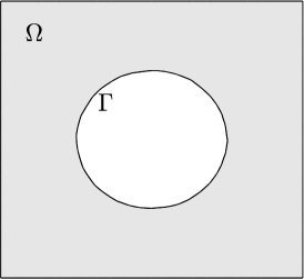
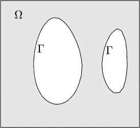
Figure 1: The final domain (left) and initial guess (right) for Model Problem 1. The gray area is the computational domain $\Omega$, the outer square boundary is fixed, and $\Gamma$ is the free boundary.

Model Problem 2.

Let $\Omega_{0}=[0,1]^{2}$ be the unit square as before and $\Omega_{1}\subset\Omega_{0}$ be a subdomain in the interior of $\Omega_{0}$ with boundary $\Gamma$. Next let $\Omega_{2}$ and $\Omega_{3}$ be the balls of radius $R=1/12$ centered in the points $(1/3,2/3)$ and $(2/3,1/3)$. Finally, set $\Omega=\Omega_{1}\setminus(\Omega_{2}\cup\Omega_{3})$ and consider the boundary conditions

$$u =1 \text{on }\partial\Omega\setminus\Gamma$$ (8.5)

$$n\cdot\nabla u =-3 \text{on }\Gamma$$ (8.6)

$$u =0 \text{on }\Gamma$$ (8.7)

In this example there is no known exact position of the free boundary. We will use a level set function corresponding to the domain Figure 2 (right sub-figure) as an initial guess.

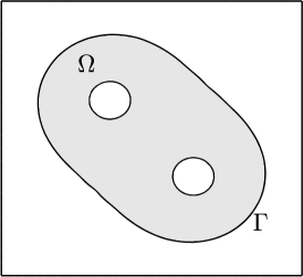
Figure 2: The final domain (left) and initial guess (right) for Model Problem 2. The gray area is the computational domain $\Omega$, the outer square boundary and the two inner most circles are fixed, and $\Gamma$ is the free bondary.

8.2 Convergence of the Velocity Field

We investigate the convergence rate of the discrete velocity field for Model Problem 1. In Figure 3 we display the error in the discrete velocity field in the $H^{1}$-norm and $L^{2}$-norm where the reference solution $\beta_{\mathrm{ref}}$ is computed on a quasi-uniform mesh with $526338$ degrees of freedom. We obtain slightly better convergence rates than $\mathcal{O}(h^{1/2})$ and $\mathcal{O}(h^{3/2})$ in $H^{1}$ and $L^{2}$-norm, respectively, which is in agreement with Theorem 7.3.

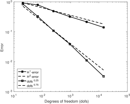
Figure 3: Convergence of the error in velocity field in Model Problem 1 in the $H^{1}$ and $L^{2}$-norm.

8.3 Free Boundary Problem

In Figure 4 and Figure 5 we present the convergence history of $R_{\Gamma}$, see (6.1), for Model Problem 1 and 2. In Figure 6 we show the approximation of $\Omega$ obtained after $0,5,15,$ and $46$ iterations, where iteration $46$ is the final domain. In Figure 6 we note that we rapidly obtain a domain which resembles the final domain, but to straighten the kinks in the boundary takes some extra effort.

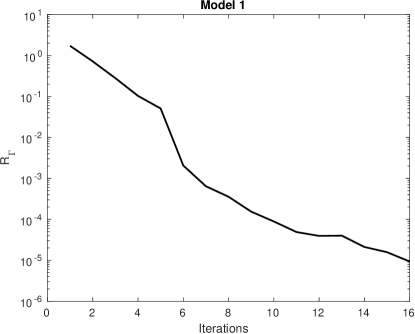
Figure 4: Convergence of $R_{\Gamma}$ for Model Problem 1.

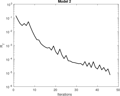
Figure 5: Convergence of $R_{\Gamma}$ for Model Problem 2.

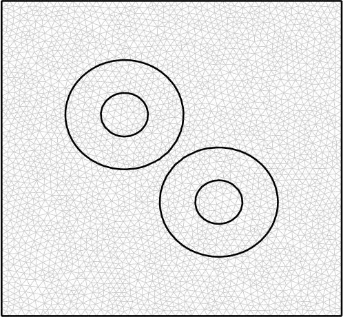
(a) Iteration 0.

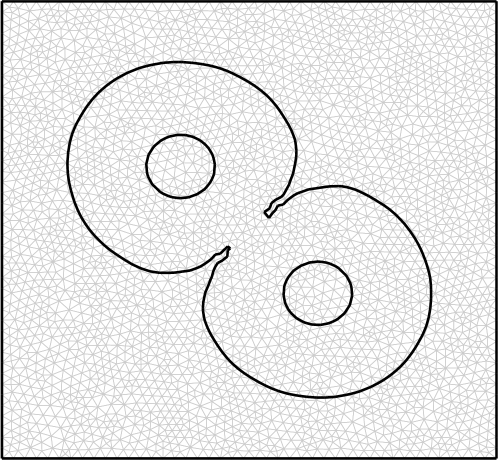
(b) Iteration 5.

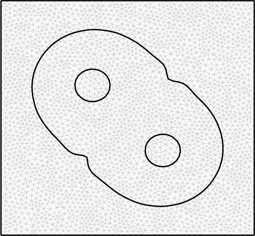
(c) Iteration 15.

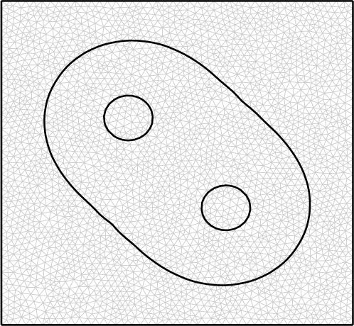
(d) Iteration 46.

Figure 6: The computational domain for Model Problem 2 after 0, 5, 15, and 46 iterations.

Appendix A Bounds for $\boldsymbol{II_{1}-II_{5}}$ in the Proof of Theorem 7.3

Term $\boldsymbol{II_{1}}$.

Dividing $II_{1}$ into three suitable terms and then using Hölder’s inequality we obtain

$$II_{1} =\int_{\Omega}(B\nabla u\cdot\nabla p-B\nabla u_{h}\cdot\nabla p_{h})\,\text{\rm d}\Omega$$ (A.1)

$$=(B\nabla(u-u_{h}),\nabla p)_{L^{2}(\Omega)}$$ (A.2)

$$\qquad+(B\nabla u,\nabla(p-p_{h}))_{L^{2}(\Omega)}$$

$$\qquad-(B\nabla(u-u_{h}),\nabla(p-p_{h}))_{L^{2}(\Omega)}$$

$$\leq\|B\|_{L^{2}(\Omega)}\|\nabla(u-u_{h})\|_{L^{2}(\Omega)}\|\nabla p\|_{L^{\infty}(\Omega)}$$ (A.3)

$$\qquad+\|B\|_{L^{2}(\Omega)}\|\nabla u\|_{L^{\infty}(\Omega)}\|\nabla(p-p_{h})\|_{L^{2}(\Omega)}$$

$$\qquad+\|B\|_{L^{2}(\Omega)}\|\nabla(u-u_{h})\|_{L^{4}(\Omega)}\|\nabla(p-p_{h})\|_{L^{4}(\Omega)}$$

$$\leq\|e_{h}\|_{H^{1}(\Omega)}h\|u\|_{W^{2}_{2}(\Omega)}\|p\|_{W^{2}_{4}(\Omega)}$$ (A.4)

$$\qquad+\|e_{h}\|_{H^{1}(\Omega)}\|u\|_{W^{2}_{4}(\Omega)}h\|p\|_{W^{2}_{2}(\Omega)}$$

$$\qquad+\|e_{h}\|_{H^{1}(\Omega)}h^{(4-d)/2}\|u\|_{W^{2}_{4}(\Omega)}\|p\|_{W^{2}_{4}(\Omega)}$$

$$\lesssim\delta\|e_{h}\|_{H^{1}(\Omega)}^{2}+\delta^{-1}\Big{(}h^{2}+h^{(4-d)}\Big{)}\|u\|^{2}_{W^{2}_{4}(\Omega)}\|p\|^{2}_{W^{2}_{4}(\Omega)}$$ (A.5)

where in (A.4) we used the a priori error estimates (7.21) and (7.38), with $p=2$ for the first two terms and with $p=4$ for the third term, and the Sobolev embedding theorem to conclude that

$$\|\nabla v\|_{L^{\infty}(\Omega)}\lesssim\|v\|_{W^{2}_{4}(\Omega)}$$ (A.6)

for $v=p$ and $v=u$ since $d\leq 3$, and finally in (A.5) we used the basic bound $\|v\|_{W^{2}_{2}(\Omega)}\lesssim\|v\|_{W^{2}_{4}(\Omega)}$ for $v=p$ and $v=u$.

Term $\boldsymbol{II_{2}}$.

Using the same approach as for Term $II_{2}$ (with $B$ replaced by $\nabla\cdot e_{h}$) we obtain

$$II_{2} \lesssim\delta\|e_{h}\|_{H^{1}(\Omega)}^{2}+\delta^{-1}h\|u\|^{2}_{W^{2}_{4}(\Omega)}\|p\|^{2}_{W^{2}_{4}(\Omega)}$$ (A.7)

Term $\boldsymbol{II_{3}}$.

Using Hölder’s inequality

$$II_{3} =\int_{\Omega}(\nabla\cdot e_{h})f(p-p_{h})\,\text{\rm d}\Omega$$ (A.8)

$$\leq\|\nabla\cdot e_{h}\|_{L^{2}(\Omega_{0})}\|f\|_{L^{4}(\Omega)}\|p-p_{h}\|_{L^{4}(\Omega)}$$ (A.9)

$$\lesssim\|e_{h}\|_{H^{1}(\Omega_{0})}\|f\|_{L^{4}(\Omega)}h^{(8-d)/4}\|p\|_{W^{2}_{4}(\Omega)}$$ (A.10)

$$\lesssim\delta\|e_{h}\|_{H^{1}(\Omega_{0})}^{2}+\delta^{-1}h^{(8-d)/2}\|f\|_{L^{4}(\Omega)}^{2}\|p\|_{W^{2}_{4}(\Omega)}^{2}$$ (A.11)

Term $\boldsymbol{II_{4}}$.

Using the conjugate rule followed by Hölder’s inequality,

$$\int_{\Gamma}(\nabla_{\Gamma}\cdot e_{h})(u^{2}-u_{h}^{2}))\,\text{\rm d}\Gamma =\int_{\Gamma}(\nabla_{\Gamma}\cdot e_{h})(u+u_{h})(u-u_{h}))\,\text{\rm d}\Gamma$$ (A.12)

$$\leq\|\nabla_{\Gamma}\cdot e_{h}\|_{L^{2}(\Gamma)}\|u+u_{h}\|_{L^{4}(\Gamma)}\|u-u_{h}\|_{L^{4}(\Gamma)}$$ (A.13)

$$\leq\delta h\|\nabla_{\Gamma}\cdot e_{h}\|_{L^{2}(\Gamma)}^{2}+\delta^{-1}h^{-1}\|u+u_{h}\|_{L^{4}(\Gamma)}^{2}\|u-u_{h}\|_{L^{4}(\Gamma)}^{2}$$ (A.14)

$$\leq\delta\|e_{h}\|_{H^{1}(\Omega_{0})}^{2}+\delta^{-1}h^{(5-d)/2}\|u\|_{W^{2}_{4}(\Omega)}^{4}$$ (A.15)

Here we used the trace inequality

$$\|v\|_{L^{p}(\Gamma)}\leq\|v\|_{L^{p}(\partial\Omega)}\lesssim\|v\|_{L^{p}(\Omega)}^{1-1/p}\|v\|_{W^{1}_{p}(\Omega)}^{1/p}\qquad v\in W^{1}_{p}(\Omega)$$ (A.16)

with $p=4$ and $v=u-u_{h}$ followed by the a priori error estimate (7.21) to conclude that

$$\|u-u_{h}\|_{L^{4}(\Gamma)} \lesssim\|u-u_{h}\|_{L^{4}(\Omega)}^{3/4}\|u-u_{h}\|_{W^{1}_{4}(\Omega)}^{1/4}$$ (A.17)

$$\lesssim(h^{(8-d)/4})^{3/4}(h^{(4-d)/4})^{1/4}\|u\|_{W^{2}_{4}(\Omega)}$$ (A.18)

$$\lesssim h^{(7-d)/4}\|u\|_{W^{2}_{4}(\Omega)}$$ (A.19)

and the following estimate

$$\|u+u_{h}\|_{L^{4}(\Gamma)} \lesssim\|u\|_{L^{4}(\Gamma)}+\|u-u_{h}\|_{L^{4}(\Gamma)}$$ (A.20)

$$\lesssim\|u\|_{L^{4}(\Gamma)}+\|u-u_{h}\|_{W^{1}_{4}(\Omega)}$$ (A.21)

$$\lesssim\|u\|_{L^{4}(\Gamma)}+h^{(4-d)/4}\|u\|_{W^{2}_{4}(\Omega)}$$ (A.22)

$$\lesssim\|u\|_{W^{2}_{4}(\Omega)}$$ (A.23)

which holds since $h\in(0,h_{0}]$.

Term $\boldsymbol{II_{5}}$.

Using Hölder’s inequality

$$II_{5} =\int_{\Gamma}(\nabla_{\Gamma}\cdot e_{h})g_{N}(p-p_{h})\,\text{\rm d}\Gamma$$ (A.24)

$$\leq\|\nabla_{\Gamma}\cdot e_{h}\|_{L^{2}(\Gamma)}\|g_{N}\|_{L^{4}(\Gamma)}\|p-p_{h}\|_{L^{4}(\Gamma)}$$ (A.25)

$$\leq\delta h\|\nabla_{\Gamma}\cdot e_{h}\|_{L^{2}(\Gamma)}^{2}+\delta h^{-1}\|g_{N}\|_{L^{4}(\Gamma)}^{2}\|p-p_{h}\|_{L^{4}(\Gamma)}^{2}$$ (A.26)

$$\leq\delta\|e_{h}\|_{H^{1}(\Omega_{0})}^{2}+h^{(5-d)/2}\|g_{N}\|_{L^{4}(\Gamma)}^{2}\|p\|_{W^{2}_{4}(\Omega)}^{2}$$ (A.27)

where in (A.27) the first term was estimated using the inverse estimate

$$h\|v\|^{2}_{L^{2}(\Gamma\cap T)}\lesssim\|v\|^{2}_{H^{1}(T)}\qquad v\in P_{1}(T)$$ (A.28)

for $T\in{\mathcal{T}_{h}}$ such that $\Gamma\cap T\neq\emptyset$ with $v=e_{h}$, and for the second term we used the estimate

$$\|p-p_{h}\|_{L^{4}(\Gamma)} \lesssim h^{(7-d)/4}\|p\|_{W^{2}_{4}(\Omega)}$$ (A.29)

which follows in the same way as in (A.17-A.19).

References

- [1] G. Allaire, C. Dapogny, and P. Frey. Shape optimization with a level set based mesh evolution method. Comput. Methods Appl. Mech. Engrg., 282:22–53, 2014.
- [2] G. Allaire, F. Jouve, and A.-M. Toader. Structural optimization by the level-set method. In Free boundary problems (Trento, 2002), volume 147 of Internat. Ser. Numer. Math., pages 1–15. Birkhäuser, Basel, 2004.
- [3] A. Beurling. On free boundary problems for the Laplace equation. Seminars on analytic functions I. Institute Advanced Studies Seminars, Princeton, 1957.
- [4] E. Burman, S. Claus, P. Hansbo, M. G. Larson, and A. Massing. CutFEM: discretizing geometry and partial differential equations. Internat. J. Numer. Methods Engrg., 104(7):472–501, 2015.
- [5] E. Burman and M. A. Fernández. Finite element methods with symmetric stabilization for the transient convection-diffusion-reaction equation. Comput. Methods Appl. Mech. Engrg., 198(33-36):2508–2519, 2009.
- [6] E. Burman and P. Hansbo. Fictitious domain finite element methods using cut elements: II. A stabilized Nitsche method. Appl. Numer. Math., 62(4):328–341, 2012.
- [7] E. Burman, P. Hansbo, M. G. Larson, and S. Zahedi. Cut finite element methods for coupled bulk–surface problems. Numer. Math., 133(2):203–231, 2016.
- [8] M. Cenanovic, P. Hansbo, and M. G. Larson. Minimal surface computation using a finite element method on an embedded surface. Internat. J. Numer. Methods Engrg., 104(7):502–512, 2015.
- [9] Z. Chen and J. Zou. Finite element methods and their convergence for elliptic and parabolic interface problems. Numer. Math., 79(2):175–202, 1998.
- [10] R. Correa and A. Seeger. Directional derivates in minimax problems. Numer. Funct. Anal. Optim., 7(2-3):145–156, 1984/85.
- [11] C. Dapogny and P. Frey. Computation of the signed distance function to a discrete contour on adapted triangulation. Calcolo, 49(3):193–219, 2012.
- [12] F. de Gournay. Velocity extension for the level-set method and multiple eigenvalues in shape optimization. SIAM J. Control Optim., 45(1):343–367, 2006.
- [13] K. Eppler, H. Harbrecht, and M. S. Mommer. A new fictitious domain method in shape optimization. Comput. Optim. Appl., 40(2):281–298, 2008.
- [14] M. Flucher and M. Rumpf. Bernoulli’s free-boundary problem, qualitative theory and numerical approximation. J. Reine Angew. Math., 486:165–204, 1997.
- [15] P. Hansbo. Nitsche’s method for interface problems in computational mechanics. GAMM-Mitt., 28(2):183–206, 2005.
- [16] P. Hansbo, M. G. Larson, and S. Zahedi. A cut finite element method for coupled bulk-surface problems on time-dependent domains. Comput. Methods Appl. Mech. Engrg., 307:96–116, 2016.
- [17] H. Harbrecht. Analytical and numerical methods in shape optimization. Math. Methods Appl. Sci., 31(18):2095–2114, 2008.
- [18] H. Harbrecht. A Newton method for Bernoulli’s free boundary problem in three dimensions. Computing, 82(1):11–30, 2008.
- [19] R. Hiptmair and A. Paganini. Shape optimization by pursuing diffeomorphisms. Comput. Methods Appl. Math., 15(3):291–305, 2015.
- [20] R. Hiptmair, A. Paganini, and S. Sargheini. Comparison of approximate shape gradients. BIT, 55(2):459–485, 2015.
- [21] T. Y. Hou. Numerical solutions to free boundary problems. Acta Numer., 4:335–415, 1995.
- [22] C. M. Kuster, P. A. Gremaud, and R. Touzani. Fast numerical methods for Bernoulli free boundary problems. SIAM J. Sci. Comput., 29(2):622–634, 2007.
- [23] A. Laurain and K. Sturm. Distributed shape derivative via averaged adjoint method and applications. ESAIM: Math. Model. Numer. Anal., 50(4):1241–1267, 2016.
- [24] S. Osher and J. A. Sethian. Fronts propagating with curvature-dependent speed: algorithms based on Hamilton-Jacobi formulations. J. Comput. Phys., 79(1):12–49, 1988.
- [25] L. R. Scott and S. Zhang. Finite element interpolation of nonsmooth functions satisfying boundary conditions. Math. Comp., 54(190):483–493, 1990.
- [26] E. Shargorodsky and J. Toland. Bernoulli free-boundary problems. Mem. Am. Math. Soc., 196(914), 2008.
- [27] J. Sokolowski and J.-P. Zolesio. Introduction to shape optimization. Springer, 1992.