Typing weak MSOL properties

Abstract.

We consider $\lambda Y$-calculus as a non-interpreted functional programming language: the result of the execution of a program is its normal form that can be seen as the tree of calls to built-in operations. Weak monadic second-order logic (wMSOL) is well suited to express properties of such trees. We give a type system for ensuring that the result of the execution of a $\lambda Y$-program satisfies a given wMSOL property. In order to prove soundness and completeness of the system we construct a denotational semantics of $\lambda Y$-calculus that is capable of computing properties expressed in wMSOL.

1. Introduction

Higher-order functional programs are more and more frequently used to write interactive applications. In this context it is important to reason about behavioral properties of programs. We present a kind of type and effect discipline [26] where a well-typed program will satisfy behavioral properties expressed in weak monadic second-order logic (wMSOL).

We consider the class of programs written in the simply-typed calculus with recursion and finite base types: the $\lambda Y$-calculus. This calculus offers an abstraction of higher-order programs that faithfully represents higher-order control. The dynamics of an interaction of a program with its environment is represented by the Böhm tree of a $\lambda Y$-term that is a tree reflecting the control flow of the program. For example, the Böhm tree of the term $Yx.ax$ is the infinite sequence of $a$’s, representing that the program does an infinite sequence of $a$ actions without ever terminating. Another example is presented in Figure 1. A functional program for the factorial function is written as a $\lambda Y$-term $\mathit{Fct}$ and the value of $\mathit{Fct}$ applied to a constant $c$ is calculated. Observe that all constants in $\mathit{Fct}$ are non-interpreted. The Böhm tree semantics reflects the call-by-name evaluation strategy. Nevertheless, the call-by-value evaluation can be encoded, so can be finite data domains and conditionals over them [15, 20, 13]. The approach is then to translate a functional program to a $\lambda Y$-term and to examine the Böhm tree it generates.

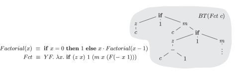
Figure 1. Böhm tree of the factorial function

Since the dynamics of the program is represented by a potentially infinite tree, monadic second-order logic (MSOL) is a natural candidate for the language to formulate properties in. This logic is an extension of first-order logic with quantification over sets. MSOL captures precisely regular properties of trees [29], and it is decidable if the Böhm tree generated by a given $\lambda Y$-term satisfies a given property [27]. In this paper we will restrict to weak monadic second-order logic (wMSOL). The difference is that in wMSOL quantification is restricted to range over finite sets. While wMSOL is a proper fragment of MSOL, it is sufficiently strong to express safety, reachability, and many liveness properties. Over sequences, that is, degenerated trees where every node has one successor, wMSOL is equivalent to full MSOL.

The basic judgments we are interested in are of the form $BT(M)\vDash\alpha$ meaning that the result of the evaluation of $M$, i.e. the Böhm tree of $M$, has the property $\alpha$ formulated in wMSOL. Going back to the example of the factorial function from Figure 1, we can consider a property: all computations that eventually take the middle branch in a node labeled by “if” are finite. This property holds in $BT(\mathit{Fct}\ c)$. Observe by the way that $BT(\mathit{Fct}\ c)$ is not regular – it has infinitely many non-isomorphic subtrees as the number of subtractions occurring in the left branches of “if” nodes is growing with the depth of those nodes. In general, the interest of judgments of the form $BT(M)\vDash\alpha$ is due to their ability to express liveness and fairness properties of executions, like: “every open action is eventually followed by a close action”, or that “there are infinitely many read actions”. Various other verification problems for functional programs can be reduced to this problem [20, 22, 28, 37, 12].

Technically, the judgment $BT(M)\vDash\alpha$ is equivalent to determining whether a Böhm tree of a given $\lambda Y$-term is accepted by a given weak alternating automaton. This problem is known to be decidable thanks to the result of Ong [27], but we hope that the denotational approach we are pursuing here brings additional benefits. Our two main contributions are:

• A construction of a finitary model for a given weak alternating automaton. The ranking condition on the automaton is lifted to the denotational model and reflected in the alternation of the least and greatest fixpoints. The value of a term in this model determines if the Böhm tree of the term is accepted by the automaton. So verification is reduced to evaluation in the model.

• Two type systems. A typing system deriving statements of the form “the value of a term $M$ is bigger than an element $d$ of the model”; and a typing system for dual properties. These typing systems use standard fixpoint rules and follow the methodology coined as Domains in Logical Form [1]. Thanks to the first item, these typing systems can directly talk about acceptance/rejection of the Böhm tree of a term by an automaton. These type systems are decidable, and every term has a “best” type that simply represents its value in the model.

Having a model and a type system has several advantages over having just a decision procedure. First, it makes verification compositional: the result for a term is calculated from the results for its subterms. In particular, it opens possibilities for a modular approach to the verification of large programs. Next, it enables semantic based program transformations as for example reflection of a given property in a given term [8, 34, 13]. It also implies the transfer theorem for wMSOL [33] with a number of consequences offered by this theorem. Finally, models open a way to novel verification algorithms be it through evaluation, type system, or through hybrid algorithms using typing and evaluation at the same time [36]. We come back to these points in the conclusions.

Related work. Historically, Ong [27] has shown the decidability of the MSOL theory of Böhm trees for all $\lambda Y$-terms. This result has been revisited in several different ways. Some approaches take a term of the base type, and unroll it to some infinite object: tree with pointers [27], computation of a higher-order pushdown automaton with collapse [14], a collection of typing judgments that are used to define a game [21], a computation of a Krivine machine [32]. Recently, Tsukada and Ong [38] have presented a compositional approach: they give a typing system where the notion of a derivation is standard, their types are extended with annotations, and the fixpoint combinator is defined via game on these types with annotations. We will comment more on the relation with this work after we introduce our type system, as well as in the conclusions. Another recent advance is given by Hofmann and Chen [11] who provide a type system for verifying path properties of trees generated by first-order $\lambda Y$-terms. In other words, this last result gives a typing system for verifying path properties of trees generated by deterministic pushdown automata. Compared to this last work, we consider the whole $\lambda Y$-calculus and an incomparable set of properties.

Already some time ago, Aehlig [2] has discovered an easy way to prove Ong’s theorem restricted to properties expressed by tree automata with trivial acceptance conditions (TAC automata). The core of his approach can be formulated by saying that the verification problem for such properties can be reduced to evaluation in a specially constructed and simple model. Later, Kobayashi proposed a type system for such properties and constructed a tool based on it [20]. This in turn opened a way to an active ongoing research resulting in the steady improvement of the capacities of the verification tools [19, 9, 10, 30]. TAC automata can express only safety properties. Our models consist of layers of models used by Aehlig, and our type system is a layered version of Kobayashi’s system. This close relation to the model and type system for trivial properties, makes us hope that our model and typing system can be useful for practical verification of wMSOL properties.

The model approach to verification of $\lambda Y$-calculus is quite recent. In [34] it is shown that simple models with greatest fixpoints capture exactly properties expressed with TAC automata. An extension is then proposed to allow one to detect divergence. The simplicity offered by models is exemplified by Haddad’s recent work [13] giving simple semantic based transformations of $\lambda Y$-terms.

We would also like to mention two other quite different approaches to integrate properties of infinite behaviors into typing. Naik and Palsberg [25] make a connection between model-checking and typing. They consider only safety properties, and since their setting is much more general than ours, their type system is more complex too. Jeffrey [17, 18] has shown how to incorporate Linear Temporal Logic into types using a much richer dependent types paradigm. The calculus is intended to talk about control and data in functional reactive programming framework, and aims at using SMT solvers.

Organization of the paper. In the next section we introduce the main objects of our study: $\lambda Y$-calculus, and weak alternating automata. Section 3 presents the type system. Its soundness and completeness can be straightforwardly formulated for closed terms of atomic type. For the proof though, we need a statement about all terms. This is where the model based approach helps. Section 4 describes how to construct models for wMSOL properties. In Section 5 we come back to our type systems. The general soundness and completeness property we prove says that types can denote every element of the model, and the type systems can derive precisely the judgments that hold in the model (Theorem 23). In the conclusion section we mention other applications of our model.

2. Preliminaries

We quickly fix notations related to the simply typed $\lambda Y$-calculus and to Böhm trees. We then recall the definition of weak alternating automata on ranked trees. These will be used to specify properties of Böhm trees. Finally, we introduce the notion of the greatest fixpoint models for the $\lambda Y$-calculus. This notion allows us to adapt the definition of recognizability from language theory, so models can be used to define sets of terms. These sets of terms are closed under the reduction rules of the $\lambda Y$-calculus. We recall the characterization, in terms of automata, of the sets of terms recognizable by the greatest fixpoint models.

The set $\mathcal{T}$ of types of $\lambda Y$-calculus is constructed from a unique basic type $o$ using a binary operation $\to$ that associates to the right. Thus $o$ is a type and if $A$, $B$ are types, so is $(A\to B)$. The order of a type is defined by: $\mathit{order}(o)=0$, and $\mathit{order}(A\to B)=max(1+\mathit{order}(A),\mathit{order}(B))$. We work with tree signatures that are finite sets of typed constants of order at most $1$. Types of order $1$ are of the form $o\to\dots\to o\to o$ that we abbreviate $o^{i}\to o$ when they contain $i+1$ occurrences of $o$. For convenience we assume that $o^{0}\to o$ is just $o$. If $\Sigma$ is a signature, we write $\Sigma^{(i)}$ for the set of constants of type $o^{i}\to o$. In examples we will often use constants of type $o\to o$ as this makes the examples more succinct. At certain times, we will restrict to the types $o$ and $o^{2}\to o$ that are representative for all the cases.

Simply typed $\lambda Y$-terms are built from the constants in the signature, and constants $Y^{A}$, $\Omega^{A}$ for every type $A$. These stand for the fixpoint combinator and undefined term, respectively. The fixpoint combinators allows to have have computations with a recursion. The undefined terms represent diverging computation, but also, at a technical level are used to construct finite approximations of infinite computations. Apart from constants, for each type $A$ there is a countable set of variables $x^{A},y^{A},\dots$. Terms are built from these constants and variables using typed application: if $M$ has type $A\to B$ and $N$ has type $A$, then $(MN)$ has type $B$; and $\lambda$-abstraction: if $M$ has type $B$ then $(\lambda x^{A}.M)$ has type $A\to B$. We shall remove unnecessary parentheses, in particular, we write sequences of applications $((N_{0}N_{1})\dots N_{n})$ as $N_{0}\dots N_{n}$ and we write sequences of $\lambda$-abstractions $\lambda x_{1}.\dots\lambda x_{n}.\ M$ with only one $\lambda$: either $\lambda x_{1}\dots x_{n}.\ M$, or even shorter $\lambda\vec{x}.\ M$. We will often write $Yx.M$ instead of $Y(\lambda x.M)$. Every $\lambda Y$-term can be written in this notation since $YN$ has the same Böhm tree as $Y(\lambda x.Nx)$, and the latter term is $Yx.(Nx)$. We write $M[x_{1}:=N_{1},\dots,x_{n}:=N_{n}]$ for the term obtained from $M$ by the simultaneous capture-avoiding substitution of $N_{1}$, …, $N_{n}$ for the variables $x_{1}$, …, $x_{n}$. All the substitutions we shall consider map variables to terms of the same type. When working with an abstract substitution $\sigma$, we write $M.\sigma$ for the term obtained by applying $\sigma$ to $M$. We use the usual operational semantics of the calculus, $\beta\delta$-reduction ($\stackrel{{\scriptstyle\ast}}{{\to}}_{\beta\delta}$) which is the reflexive transitive closure of the union of the relations of $\beta$-contraction ($\to_{\beta}$) and $\delta$-contraction ($\to_{\delta}$) which are the following rewriting relations:

$$(\lambda x.M)N\to_{\beta}M[x:=N]\quad YM\to_{\delta}M(YM)$$

The Böhm tree of a term $M$ is a possibly infinite labeled tree that is defined co-inductively. If $M$ can be reduced so as to obtain a term of the form $\lambda\vec{x}.N_{0}N_{1}\dots N_{k}$ with $N_{0}$ a variable or a constant, then $BT(M)$ is a tree whose root is labeled by $\lambda\vec{x}.N_{0}$ and the immediate successors of its root are $BT(N_{1})$, …, $BT(N_{k})$. Otherwise $BT(M)$ is a single node tree whose root is labeled $\Omega^{A}$, where $A$ is the type of $M$. Böhm trees are infinite normal forms of $\lambda Y$-terms. A Böhm tree of a closed term of type $o$ over a tree signature is a potentially infinite ranked tree: a node labeled by a constant $a$ of type $o^{i}\to o$ has $i$ successors (c.f. Figure 1).

As an example take $(YF.\ N)a$ where $N=\lambda g.g(b(F(\lambda x.g(g\,x))))$. Both $a$ and $b$ have the type $o\to o$; while $F$ has type $(o\to o)\to o$, and so does $N$. Observe that we are using a more convenient notation $YF$ here. The Böhm tree of $(YF.N)a$ is $BT((YF.N)a)=aba^{2}ba^{4}b\dots a^{2^{n}}b\dots$ after every consecutive occurrence of $b$ the number of occurrences of $a$ doubles because of the double application of $g$ inside $N$.

wMSOL and weak alternating automata

We will be interested in properties of trees expressed in weak monadic second-order logic. This is an extension of first-order logic with quantification over finite sets of elements. The interplay of negation and quantification allows the logic to express many infinitary properties. The logic is closed for example under constructs: “for infinitely many vertices a given property holds”, “every path consisting of vertices having a given property is finite”. From the automata point of view, the expressive power of the logic is captured by weak alternating automata.

A weak alternating automaton works on trees over a fixed tree signature $\Sigma$. It is a tuple:

$$\mathcal{A}=\langle Q,\Sigma,q^{0}\in Q,\{\delta_{i}\}_{i\in\mathbb{N}},\rho:Q\to\mathbb{N}\rangle$$

where $Q$ is a finite set of states, $q^{0}\in Q$ is the initial state, $\rho$ is the rank function, and $\delta_{i}:Q\times\Sigma^{(i)}\to\mathcal{P}(\mathcal{P}(Q)^{i})$ is the transition function. For $q$ in $Q$, we call $\rho(q)$ its rank. The automaton is weak in the sense that when $(S_{1},\dots,S_{i})$ is in $\delta_{i}(q,a)$, then the rank of every $q^{\prime}$ in $\bigcup_{1\leq j\leq i}S_{j}$ is not bigger than the rank of $q$, i.e. $\rho(q^{\prime})\leq\rho(q)$.

Observe that since $\Sigma$ is finite, only finitely many $\delta_{i}$ are non-empty functions. From the definition it follows that $\delta_{2}:Q\times\Sigma^{(2)}\to\mathcal{P}(\mathcal{P}(Q)\times\mathcal{P}(Q))$ and $\delta_{0}:Q\times\Sigma^{(0)}\to\{\emptyset,\{()\}\}$. We will simply write $\delta$ without a subscript when this causes no ambiguity.

Automata will work on $\Sigma$-labeled trees that are partial functions $t:\mathbb{N}^{*}\stackrel{{\scriptstyle\cdot}}{{\to}}\Sigma\cup\{\Omega\}$ whose domain of definition satisfies the usual requirements, and such that the number successors of a node is determined by the label of the node. In particular, if $t(u)\in\Sigma^{(0)}\cup\{\Omega\}$ then $u$ is a leaf.

The acceptance of a tree is defined in terms of games between two players that we call Eve and Adam. A play between Eve and Adam from some node $v$ of a tree $t$ and some state $q\in Q$ proceeds as follows. If $v$ is a leaf and is labeled by some $c\in\Sigma^{(0)}$ then Eve wins iff $\delta_{0}(q,c)$ holds (i.e. $\delta_{0}(q,c)$ is not empty). If $v$ is labeled by $\Omega$ then Eve wins iff the rank of $q$ is even. Otherwise, $v$ is an internal node: Eve chooses a tuple of sets of states $(S_{1},\dots,S_{i})\in\delta(q,t(v))$; then Adam chooses $S_{j}$ (for $j=1,\dots,i$) and a state $q^{\prime}\in S_{j}$. The play continues from the $j$-th son of $v$ and state $q^{\prime}$. When a player is not able to play any move, he/she looses. If the play is infinite then the winner is decided by looking at ranks of states appearing on the play. Due to the weakness of $\mathcal{A}$, the rank of states in a play can never increase, so it eventually stabilizes at some value. Eve wins if this value is even. A tree $t$ is accepted by $\mathcal{A}$ from a state $q\in Q$ if Eve has a winning strategy in the game started from the root of $t$ and from $q$.

Automata with trivial acceptance conditions, as considered by Kobayashi [19], are obtained by requiring that all states have rank $0$. Automata with co-trivial conditions are just the ones where all states have rank $1$.

Observe that without a loss of generality we can assume that $\delta$ is monotone, i.e. if $(S_{1},\dots,S_{i})\in\delta(q,a)$ then for every $(S^{\prime}_{1},\dots,S^{\prime}_{i})$ such that $S_{j}\subseteq S^{\prime}_{j}\subseteq\{q^{\prime}:\rho(q^{\prime})\leq\rho(q)\}$ we have $(S^{\prime}_{1},\dots,S^{\prime}_{i})\in\delta(q,a)$. Indeed, adding the transitions needed to satisfy the monotonicity condition does not give Eve more winning possibilities.

An automaton defines a language of closed terms of type $o$, it consists of terms whose Böhm trees are accepted by the automaton from its initial state $q^{0}$:

$$L(\mathcal{A})=\{M\,:\,\text{$M$ is closed term of type $o$, $BT(M)$ is accepted by $\mathcal{A}$ from $q^{0}$}\}\ .$$

Observe that $L(\mathcal{A})$ is closed under $\beta\delta$-conversion since the Church-Rosser property of the calculus implies that two $\beta\delta$-convertible terms have the same Böhm tree.

Consider a weak alternating automaton $\mathcal{A}$ defining the property “action $b$ appears infinitely often”. The automaton has states $Q=\{q_{1},q_{2}\}$, and the signature $\Sigma=\{a,b\}$ consisting of two constants of type $o\to o$. Over this signature, the Böhm trees are just sequences. The transitions of $\mathcal{A}$ are:

$$\delta(q_{1},a) =\{q_{1}\} \delta(q_{2},a) =\{q_{1},q_{2}\}$$

$$\delta(q_{1},b) =\emptyset \delta(q_{2},b) =\{q_{2}\}$$

The ranks of states are indicated by their subscripts. When started in $q_{2}$ the automaton spawns a run from $q_{1}$ each time it sees letter $a$. The spawned runs must stop in order to accept, and they stop when they see letter $b$ (cf. Figure 2). So every $a$ must be eventually followed by $b$.

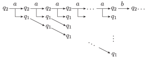
Figure 2. A run of an alternating automaton on $a\dots ab\dots$

Models.

We use standard notions and notations for models for $\lambda Y$-calculus, in particular for valuation/variable assignment and of interpretation of a term (see [16]). We shall write ${[\![M]\!]}^{\mathcal{S}}_{\nu}$ for the interpretation of a term $M$ in a model $\mathcal{S}$ with the valuation $\nu$. As usual, we will omit subscripts or superscripts in the notation of the semantic function if they are clear from the context.

The simplest models of $\lambda Y$-calculus are based on monotone functions. A GFP-model of a signature $\Sigma$ is a tuple $\mathcal{S}=\langle\{\mathcal{S}_{A}\}_{A\in\mathcal{T}},\rho\rangle$ where $\mathcal{S}_{o}$ is a finite lattice, called the base set of the model, and for every type $A\to B\in\mathcal{T}$, $\mathcal{S}_{A\to B}$ is the lattice $\mathrm{mon}[\mathcal{S}_{A}\mapsto\mathcal{S}_{B}]$ of monotone functions from $\mathcal{S}_{A}$ to $\mathcal{S}_{B}$ ordered coordinate-wise. The valuation function $\rho$ is required to interpret $\Omega^{A}$ as the greatest element of $\mathcal{S}_{A}$, and $Y^{A}$ as the greatest fixpoint operator of functions in $\mathcal{S}_{A\to A}$. Observe that every $\mathcal{S}_{A}$ is finite, hence all the greatest fixpoints exist without any additional assumptions on the lattice.

We can now adapt the definition of recognizability by semigroups taken from language theory to our richer models. A GFP model $\mathcal{S}$ over the base set $\mathcal{S}_{o}$ recognizes a language $L$ of closed $\lambda Y$-terms of type $o$ if there is a subset $F\subseteq\mathcal{S}_{o}$ such that $L=\{M\mid{[\![M]\!]}^{\mathcal{S}}\in F\}$. A direct consequence of Statman’s finite completeness theorem [35] is that such models can characterize a term up to equality: $BT(M)=BT(N)$ iff the values of $M$ and $N$ are the same in every monotone models. This property is sufficient for our purposes. The celebrated result of Loader [24] implies that we cannot hope for a much stronger completeness property, and have good algorithmic qualities at the same time.

The following theorem characterizes the recognizing power of GFP models.

Theorem 1 ([34]).

A language $L$ of $\lambda Y$-terms is recognized by a GFP-model iff it is a boolean combination of languages recognized by weak automata whose all states have rank $0$.

3. Type systems for wMSOL

In this section we describe the main result of the paper. We present a type system to reason about wMSOL properties of Böhm trees of terms. We will rely on the equivalence of wMSOL and weak alternating automata, and construct a type system for an automaton. For a fixed weak alternating automaton $\mathcal{A}$ we want to characterize the terms whose Böhm trees are accepted by $\mathcal{A}$, i.e. the set $L(\mathcal{A})$. The characterization will be purely type theoretic (cf. Theorem 2).

Fix an automaton $\mathcal{A}=\langle Q,\Sigma,q^{0},\{\delta_{i}\}_{i\in\mathbb{N}},\rho\rangle$. Let $m$ be the maximal rank, i.e., the maximal value $\rho$ takes on $Q$. For every $0\leq k\leq m$ we write $Q_{k}=\{q\in Q:\rho(q)=k\}$ and $Q_{\leq k}=\{q\in Q:\rho(q)\leq k\}$.

The type system we propose is obtained by allowing the use of intersections inside simple types. This idea has been used by Kobayashi [20] to give a typing characterization for languages of automata with trivial acceptance conditions. We work with, more general, weak acceptance conditions, and this will be reflected in the stratification of types, and two fixpoint rules: greatest fixpoint rule for even strata, and the least fixpoint rule for odd strata.

First, we define the sets of intersection types. They are indexed by a rank of the automaton and by a simple type. Note that every intersection type will have a corresponding simple type; this is a crucial difference with intersection types characterizing strongly normalizing terms [4]. Letting $\mathrm{Types}^{k}_{A}=\bigcup_{0\leq l\leq k}\mathrm{types}^{l}_{A}$ we define:

The difference with simple types is that now we have a set constructor that will be interpreted as the intersection of its elements. This technical choice amounts to quotient types with respect to the associativity, the commutativity and the idempotency of the intersection operator. A nice consequence in our context is that the sets $\mathrm{types}^{k}_{A}$ and $\mathrm{Types}^{k}_{A}$ are finite. Notice also that the application of the intersection type operator to two sets of types is then represented by the union of those two sets.

Suppose that in $Q$ we have states $q_{0},r_{0},q_{1}$ with ranks given by their subscripts. A type $\{q_{0},r_{0}\}\subseteq\mathrm{Types}^{0}_{o}$ will type terms whose Böhm tree is accepted both from $q_{0}$ and from $r_{0}$. A type $\{\{q_{0},r_{0}\}\to\{q_{1}\}\}\subseteq\mathrm{types}^{1}_{o\to o}$ will type terms that when given a term of type $\{q_{0},r_{0}\}$ produce a Böhm tree accepted from $q_{1}$. Observe that, for example, $\{\{q_{0},r_{0}\}\to\{q_{1}\},\{q_{1}\}\to\{q_{1}\}\}\subseteq\mathrm{Types}^{1}_{o\to o}$ while $\{\{q_{1}\},\{q_{1}\}\to\{q_{1}\}\}$ is not an intersection type in our sense since the two types in the set have different underlying simple types.

When we write $\mathrm{types}_{A}$ or $\mathrm{Types}_{A}$ we mean $\mathrm{types}^{m}_{A}$ and $\mathrm{Types}^{m}_{A}$ respectively; where $m$ is the maximal rank used by the automaton $\mathcal{A}$.

For $S\subseteq\mathrm{Types}^{k}_{A}$ and $T\subseteq\mathrm{types}^{k}_{B}$ we write $S\to T$ for $\{S\to t:t\in T\}$. Notice that $S\to T$ is included in $\mathrm{types}^{k}_{A\to B}$.

We now give subsumption rules that express the intuitive dependence between types. So as to make the connection with the model construction later, we have adopted an ordering of intersection types that is dual to the usual one (the first rule can be derived from the second and third one, but we find it more intuitive to explicitly spell it out). Usually in intersection types, the lower a type is in the subsumption order, the less terms it can type. Here we take the information order instead, the lower a type is in the subsumption order, the less precise it is. As we said earlier, this choice is motivated by the connection of types with models, the information order gives us an isomorphism between the two, while the usual choice would give us a duality between types and models.

tensy $\displaystyle\penalty 1S\subseteq T\subseteq Q$   $\displaystyle S\sqsubseteq_{o}T$   tensy $\displaystyle\penalty 1\forall s\in S,\exists t\in T,s\sqsubseteq_{A}t$   $\displaystyle S\sqsubseteq_{A}T$   tensy $\displaystyle\penalty 1s=t$   $\displaystyle s\sqsubseteq_{o}t$   tensy $\displaystyle\penalty 1T\sqsubseteq_{A}S\quad s\sqsubseteq_{B}t$   $\displaystyle S\to s\sqsubseteq_{A\to B}T\to t$

Given $S\subseteq\mathrm{Types}_{A\to B}$ and $T\subseteq\mathrm{Types}_{A}$ we write $S(T)$ for the set $\{t:(U\to t)\in S\text{ and }U\sqsubseteq T\}$.

The typing system presented in Figure 3 derives judgments of the form $\Gamma\vdash M\geq S$ where $\Gamma$ is an environment containing all the free variables of the term $M$, and $S\subseteq\mathrm{Types}_{A}$ with $A$ the type of $M$. As usual, an environment $\Gamma$ is a finite list $x_{1}\geq S_{1},\dots,x_{n}\geq S_{n}$ where $x_{1},\dots,x_{n}$ are pairwise distinct variables of type $A_{i}$, and $S_{i}\subseteq\mathrm{Types}_{A_{i}}$. We will use a functional notation and write $\Gamma(x_{i})$ for $S_{i}$. We shall also write $\Gamma,x\geq S$ for an extension of the environment $\Gamma$ with the declaration $x\geq S$.

The rules in the first row of Figure 3 express standard intersection types dependencies: the axiom, the intersection rule and the subsumption rule. The rules in the second line are specific to our fixed automaton. The third line contains the usual rules for application and abstraction with the caveat that the abstraction rule incorporates the stratification of types with respect to ranks so that the types used in the judgment are always well-formed. The least fixpoint rule in the next line is standard, it expresses that the least fixpoint can be approximated by iterations started in the least element: if we derive $\Gamma\vdash\lambda x.M\geq\emptyset\to T$ then we obtain that $\Gamma\vdash Yx.M\geq T$, that can allow us to derive $\Gamma\vdash Yx.M\geq T^{\prime}$ provided $\Gamma\vdash\lambda x.M\geq T\to T^{\prime}$ etc. The greatest fixpoint rule in the last line is more intricate. It is allowed only on even strata. If taken for $k=0$ the rule becomes the standard rule for the greatest fixpoint as the set $T$ must be the empty set. For $k>0$ the rule permits to incorporate $T$ that is the result of the fixpoint computation on the lower stratum.

tensy   $\displaystyle\Gamma,x\geq S\vdash x\geq S$  tensy $\displaystyle\penalty 1\Gamma\vdash M\geq S\quad\Gamma\vdash M\geq T$   $\displaystyle\Gamma\vdash M\geq S\cup T$  tensy $\displaystyle\penalty 1\Gamma\vdash M\geq S\quad T\sqsubseteq S$   $\displaystyle\Gamma\vdash M\geq T$

tensy   $\displaystyle\Gamma\vdash c\geq\{q:\delta_{0}(q,c)\neq\emptyset\}$  tensy $\displaystyle\penalty 1(S_{1},\dots,S_{i})\in\delta_{i}(a,q)$   $\displaystyle\Gamma\vdash a\geq\{S_{1}\to\dots\to S_{i}\to q\}$

tensy $\displaystyle\penalty 1\Gamma\vdash M\geq S\quad\Gamma\vdash N\geq T$   $\displaystyle\Gamma\vdash MN\geq S(T)$  tensy $\displaystyle\penalty 1S\subseteq\mathrm{Types}^{k},\,T\subseteq\mathrm{types}^{k}\quad\Gamma,x\geq S\vdash M\geq T$   $\displaystyle\Gamma\vdash\lambda x.M\geq S\to T$

tensy $\displaystyle\penalty 1\Gamma\vdash(\lambda x.M)\geq S\quad\Gamma\vdash(Yx.M)\geq T$  $Y\,\mathit{odd}$ $\displaystyle\Gamma\vdash Yx.M\geq S(T)$

tensy $\displaystyle\penalty 1S\subseteq\mathrm{types}^{2k}_{A},\quad T\subseteq\mathrm{Types}^{2k-1}_{A},\quad\Gamma\vdash\lambda x.M\geq(S\cup T)\to S\quad\Gamma\vdash Yx.M\geq T$  $Y\,\mathit{even}$ $\displaystyle\Gamma\vdash Yx.M\geq S\cup T$

Figure 3. Type system

Our main result says that the typing in this system is equivalent to accepting with our fixed weak alternating automaton.

Theorem 2.

For every closed term $M$ of type $o$ and every state $q$ of $\mathcal{A}$: the judgment $\vdash M\geq q$ is derivable iff $\mathcal{A}$ accepts $BT(M)$ from $q$.

Since there are finitely many types, this typing system is decidable. As we will see in the following example, this type system allows us to prove in a rather simple manner properties of Böhm trees that are beyond the reach of trivial automata. Compared to Kobayashi and Ong type system [21] and to Tsukada and Ong type system [38], the fixpoint typing rules we propose do not refer to an external parity game. Our type system does not require flagged types, and is on the contrary based on a standard treatment of free variables. In the example below we use fixpoint rules on terms of order $2$.

In order to prove Theorem 2 we will need to formulate and prove a more general statement that concerns terms of all types (Theorem 23). To describe the properties of the type system in higher types, we will construct a model from our fixed automaton $\mathcal{A}$, and show (Theorem 14) that the model recognizes $L(\mathcal{A})$ in the sense of Definition 2. Then Theorem 23 will say that the type system reflects the values of the terms in the model.

Due to the symmetries in weak alternating automata, and in the model we are going to construct, we will obtain also a dual type system. This system can be used to show that the Böhm tree of a term is not accepted by the automaton.

tensy $\displaystyle\penalty 1S\subseteq T\subseteq Q$   $\displaystyle S\sqsupseteq_{o}T$   tensy $\displaystyle\penalty 1\forall s\in S,\exists t\in T,s\sqsupseteq_{A}t$   $\displaystyle S\sqsupseteq_{A}T$   tensy $\displaystyle\penalty 1s=t$   $\displaystyle s\sqsupseteq_{o}t$   tensy $\displaystyle\penalty 1T\sqsupseteq_{A}S\quad s\sqsupseteq_{B}t$   $\displaystyle S\to s\sqsupseteq_{A\to B}T\to t$

tensy   $\displaystyle\Gamma\vdash c\geq\{q:\delta_{o}(q,c)=\emptyset\}$  tensy $\displaystyle\penalty 1\forall(S_{1},S_{2})\in\delta(a,q),(T_{1}\cap S_{1})\cup(T_{2}\cap S_{2})\neq\emptyset$   $\displaystyle\Gamma\vdash a\ngeq T_{1}\to T_{2}\to q$

tensy $\displaystyle\penalty 1\Gamma\vdash M\ngeq S\quad\Gamma\vdash N\ngeq T$   $\displaystyle\Gamma\vdash MN\ngeq S(T)$  tensy $\displaystyle\penalty 1S\in\mathrm{Types}^{k},\,T\subseteq\mathrm{types}^{k}\quad\Gamma,x\ngeq S\vdash M\ngeq T$   $\displaystyle\Gamma\vdash\lambda x.M\ngeq S\to T$

tensy $\displaystyle\penalty 1S\subseteq\mathrm{types}^{2k+1}_{A},\quad T\in\mathrm{Types}^{2k}_{A},\quad\Gamma\vdash\lambda x.M\ngeq(S\cup T)\to S\quad\Gamma\vdash Yx.M\ngeq T$  $Y\,\mathit{odd}$ $\displaystyle\Gamma\vdash Yx.M\ngeq S\cup T$

tensy $\displaystyle\penalty 1\Gamma\vdash(\lambda x.M)\ngeq S\quad\Gamma\vdash(Yx.M)\ngeq T$  $Y\,\mathit{even}$ $\displaystyle\Gamma\vdash Yx.M\ngeq S(T)$

Figure 4. Dual type system

The dual type system is presented in Figure 4 on page 4. The notation is as before but we now define $S(T)$ to be $\{s:U\to s\in S\land U\sqsupseteq T\}$. The rules for application, abstraction and variable do not change. By duality we obtain:

Corollary 3.

For every closed term $M$ of type $o$ and every state $q$ of $\mathcal{A}$: judgment $\vdash M\ngeq q$ is derivable iff $\mathcal{A}$ does not accept $BT(M)$ from $q$.

So the two type systems together allow us to derive both positive and negative information about a program.

We finish this section with two moderate size examples of typing derivations.

Take a signature consisting of two constants $c:o$ and $a:o\to o$. We consider an extremely simple weak alternating automaton with just one state $q$ of rank $1$ and transitions:

$$\delta(q,a)=\{q\}\qquad\delta(q,c)=\emptyset\ .$$

This automaton accepts the finite sequences of $a$’s ending in $c$. Observe that these transition rules give us typing axioms

tensy   $\displaystyle\vdash a\geq\{q\}\to q$   tensy   $\displaystyle\vdash c\geq q$

Notice that we omit some set parenthesis over singletons; so for example we write $c\geq q$ instead of $c\geq\{q\}$. In this example we will still keep the parenthesis to the left of the arrow to emphasize that we are in our type system, and not in simple types. In the next example we will omit them too.

First, let us look at a term $G_{1}\equiv\lambda f^{o\to o}\lambda x^{o}.\ f(fx)$. It has a simple type $\tau_{1}\equiv(o\to o)\to o\to o$. The judgment $\vdash G_{1}\geq\gamma_{1}$ is derivable in our system; where $\gamma_{1}\equiv\{\{q\}\to q\}\to\{q\}\to q$.

tensy $\displaystyle\penalty 1\hskip 5.0pt plus 1.0fil{tensy\vbox{\hbox spread0.0pt{\hskip 0.0pt plus 0.0001fil\hbox{$\displaystyle\penalty 1\Gamma\vdash f\geq\{q\}\to q\quad\hskip 5.0pt plus 1.0fil{tensy\vbox{\hbox spread0.0pt{\hskip 0.0pt plus 0.0001fil\hbox{$\displaystyle\penalty 1\Gamma\vdash f\geq\{q\}\to q\quad\Gamma\vdash x\geq q$}\hskip 0.0pt plus 0.0001fil}\hbox{\hbox{\kern 0.0pt\vrule height=0.25002pt,depth=0.25002pt,width=113.65585pt\hbox{}}}\hbox{\kern 32.94783pt\hbox{$\displaystyle\Gamma\vdash fx\geq q$}}}}\hskip 5.0pt plus 1.0fil\penalty 2$}\hskip 0.0pt plus 0.0001fil}\hbox{\hbox{\kern 0.0pt\vrule height=0.25002pt,depth=0.25002pt,width=219.74258pt\hbox{}}}\hbox{\kern 79.11617pt\hbox{$\displaystyle\Gamma\vdash f(fx)\geq q$}}}}\hskip 5.0pt plus 1.0fil\penalty 2$   $\displaystyle\vdash\lambda f\lambda x.\ f(fx)\geq\gamma_{1}$

here $\Gamma\equiv f\geq\{q\}\to q,\ x\geq q$.

Consider now $G_{2}\equiv\lambda f^{\tau_{1}}\lambda x^{o\to o}.\ f(fx)$. We have that $G_{2}$ is of type $\tau_{2}\equiv\tau_{1}\to\tau_{1}$. A derivation very similar to the above will show $\vdash G_{2}\geq\gamma_{2}$ where $\gamma_{2}\equiv\{\gamma_{1}\}\to\gamma_{1}$.

Then by induction we can define $G_{i}\equiv\lambda f^{\tau_{i-1}}\lambda x^{\tau_{i-2}}.\ f(fx)$ that is of a type $\tau_{i}\equiv\tau_{i-1}\to\tau_{i-1}$. Still a similar derivation as above will show $\vdash G_{i}\geq\gamma_{i}$ where $\gamma_{i}\equiv\{\gamma_{i-1}\}\to\gamma_{i-1}$.

One use of application rule then shows that $G_{i}G_{i-1}\geq\gamma_{i-1}$:

tensy $\displaystyle\penalty 1\vdash G_{i}\geq\{\gamma_{i-1}\}\to\gamma_{i-1}\quad\vdash G_{i-1}\geq\gamma_{i-1}$   $\displaystyle\vdash G_{i}G_{i-1}\geq\gamma_{i-1}$

In consequence, we can construct by induction a derivation of

$$\vdash G_{i}G_{i-1}\dots G_{1}ac\geq q$$

This derivation proves that the Böhm tree of $G_{i}G_{i-1}\dots G_{1}ac$ is a sequence of $a$’s ending in $c$. While the length of this sequence is a tower of exponentials in the height $i$, the typing derivation we have constructed is linear in $i$ (if types are represented succinctly). This simple example, already analyzed in [20], shows the power of modular reasoning provided by the typing approach. We should note though that if the initial automaton had two states, the number of potential types would also be roughly the tower of exponentials in $i$. Due to the complexity bounds [36], there are terms and automata for which there is no small derivation. Yet one can hope that in many cases a small derivation exists. For example, if we wanted to show that the length of the sequence is even then the automaton would have two states but the derivation would be essentially the same.

Consider the term $M=(YF.N)a$ where $N=\lambda g.g(b(F(\lambda x.g(g\,x))))$. As we have seen on page 2, $BT(M)=aba^{2}ba^{4}b\dots a^{2^{n}}b\dots$. We show with typing that there are infinitely many occurrences of $b$ in $BT(M)$. To this end we take an automaton having states $Q=\{q_{1},q_{2}\}$, and working over the signature containing $a$ and $b$. The transitions of the automaton are:

$$\delta(q_{1},a)=\{q_{1}\},\quad\delta(q_{2},a)=\{q_{1},q_{2}\},\quad\delta(q_{1},b)=\emptyset,\quad\delta(q_{2},b)=q_{2}\ .$$

The ranks of states are indicated by their subscripts. Starting with state $q_{2}$, the automaton only accepts sequences that contain infinitely many $b$’s. So our goal is to derive $\vdash(YF.N)a\geq q_{2}$. First observe that from the definition of the transitions of the automaton we get axioms:

tensy   $\displaystyle\vdash a\geq q_{1}\to q_{1}$  tensy   $\displaystyle\vdash a\geq\{q_{1},q_{2}\}\to q_{2}$  tensy   $\displaystyle\vdash b\geq\emptyset\to q_{1}$  tensy   $\displaystyle\vdash b\geq q_{2}\to q_{2}$

Looking at the typings of $a$, we can see that we will get our desired judgment from the application rule if we prove:

$$\small\vdash YF.N\geq S\qquad\text{where $S$ is $\{q_{1}\to q_{1},\{q_{1},q_{2}\}\to q_{2}\}\to q_{2}$.}$$

To this end, we apply the subsumption rule and the greatest fixpoint rule:

tensy $\displaystyle\penalty 1\hskip 4.5pt plus 1.0fil{tensy\vbox{\hbox spread0.0pt{\hskip 0.0pt plus 0.0001fil\hbox{$\displaystyle\penalty 1\vdash\lambda F.N\geq(S\cup T)\to S\quad\vdash YF.N\geq T$}\hskip 0.0pt plus 0.0001fil}\hbox{\hbox{\kern 0.0pt\vrule height=0.25002pt,depth=0.25002pt,width=152.0688pt\hbox{\kern 2.70003pt$Y\,\textit{even}$}}}\hbox{\kern 40.77345pt\hbox{$\displaystyle\vdash YF.N\geq S\cup T$}}}}\hskip 4.5pt plus 1.0fil\penalty 2$   $\displaystyle\vdash YF.N\geq S$   where $T=\{(q_{1}\to q_{1})\to q_{1}\}$

The derivation of the top right judgment uses the least fixpoint rule:

tensy $\displaystyle\penalty 1\hskip 4.5pt plus 1.0fil{tensy\vbox{\hbox spread0.0pt{\hskip 0.0pt plus 0.0001fil\hbox{$\displaystyle\penalty 1\hskip 4.5pt plus 1.0fil{tensy\vbox{\hbox spread0.0pt{\hskip 0.0pt plus 0.0001fil\hbox{$\displaystyle\penalty 1\hskip 4.5pt plus 1.0fil{tensy\vbox{\hbox spread0.0pt{\hskip 0.0pt plus 0.0001fil\hbox{\kern 41.3369pt\hbox{$\displaystyle\penalty 1$}}\hskip 0.0pt plus 0.0001fil}\hbox{\hbox{\kern 0.0pt\vrule height=0.25002pt,depth=0.25002pt,width=82.6738pt\hbox{}}}\hbox{\kern 0.0pt\hbox{$\displaystyle g\geq q_{1}\to q_{1}\vdash g\geq q_{1}\to q_{1}$}}}}\hskip 4.5pt plus 1.0fil\penalty 2\quad g\geq q_{1}\to q_{1}\vdash b(F(\lambda x.g(g\,x)))\geq q_{1}$}\hskip 0.0pt plus 0.0001fil}\hbox{\hbox{\kern 0.0pt\vrule height=0.25002pt,depth=0.25002pt,width=248.83704pt\hbox{}}}\hbox{\kern 55.42757pt\hbox{$\displaystyle g\geq q_{1}\to q_{1}\vdash g(b(F(\lambda x.g(g\,x))))\geq q_{1}$}}}}\hskip 4.5pt plus 1.0fil\penalty 2$}\hskip 0.0pt plus 0.0001fil}\hbox{\hbox{\kern 0.0pt\vrule height=0.25002pt,depth=0.25002pt,width=279.63397pt\hbox{}}}\hbox{\kern 49.55725pt\hbox{$\displaystyle\vdash\lambda F\lambda g.g(b(F(\lambda x.g(g\,x))))\geq\emptyset\to(q_{1}\to q_{1})\to q_{1}$}}}}\hskip 4.5pt plus 1.0fil\penalty 2$  $Y\,\mathit{odd}$ $\displaystyle\vdash YF.N\geq(q_{1}\to q_{1})\to q_{1}$

We have displayed only one of the two premises of the $Yodd$ rule since the other is of the form $\geq\emptyset$ so it is vacuously true. The top right judgment is derivable directly from the axiom on $b$. The derivation of the remaining judgment $\vdash\lambda F.N\geq(S\cup T)\to S$ is as follows.

tensy $\displaystyle\penalty 1\hskip 4.5pt plus 1.0fil{tensy\vbox{\hbox spread0.0pt{\hskip 0.0pt plus 0.0001fil\hbox{$\displaystyle\penalty 1\hskip 4.5pt plus 1.0fil{tensy\vbox{\hbox spread0.0pt{\hskip 0.0pt plus 0.0001fil\hbox{\kern 35.91129pt\hbox{$\displaystyle\penalty 1$}}\hskip 0.0pt plus 0.0001fil}\hbox{\hbox{\kern 0.0pt\vrule height=0.25002pt,depth=0.25002pt,width=71.82257pt\hbox{}}}\hbox{\kern 0.0pt\hbox{$\displaystyle\Gamma\vdash g\geq\{q_{1},q_{2}\}\to q_{2}$}}}}\hskip 4.5pt plus 1.0fil\penalty 2\par\quad\Gamma\vdash b(F(\lambda x.g(g\,x)))\geq q_{1},q_{2}$}\hskip 0.0pt plus 0.0001fil}\hbox{\hbox{\kern 0.0pt\vrule height=0.25002pt,depth=0.25002pt,width=219.63455pt\hbox{}}}\hbox{\kern 55.43227pt\hbox{$\displaystyle\Gamma\vdash g(b(F(\lambda x.g(g\,x))))\geq q_{2}$}}}}\hskip 4.5pt plus 1.0fil\penalty 2$   $\displaystyle\vdash\lambda F\lambda g.g(b(F(\lambda x.g(g\,x))))\geq(S\cup T)\to S$

where $\Gamma$ is $F\geq S\cup T,g\geq\{q_{1}\to q_{1},\{q_{1},q_{2}\}\to q_{2}\}$. So the upper left judgment is an axiom. The other judgment on the top is an abbreviation of two judgments: one to show $\geq q_{1}$ and the other one to show $\geq q_{2}$. These two judgments are proved directly using application and intersection rules.

4. Models for weak automata

We describe a construction of a model that recognizes, in a sense of Definition 2, the language defined by a weak automaton. The model depends only on the states of the automaton and their ranks. The transitions of the automaton will be encoded in the interpretation of constants. We shall work with (finite) complete lattices and with monotone functions between complete lattices. In the first subsection we define the basic structure of the model. Its properties will allow us later to define fixpoints and show that indeed we can interpret the $\lambda Y$-calculus in the model. In the last subsection we will show that with an appropriate interpretation of constants the model can recognize the language of a given weak automaton.

The challenge in this construction comes from the fact that using only the least or only the greatest fixpoints is not sufficient. Indeed, we have shown in [34] that extremal fixpoints in finitary models of $\lambda Y$-calculus capture precisely boolean combinations of properties expressed by automata with trivial acceptance conditions. The structure of a weak automaton will help us here. For the sake of the discussion let us fix an automaton $\mathcal{A}$, and let $\mathcal{A}_{\leq k}$ stand for $\mathcal{A}$ restricted to states of rank at most $k$. Ranks stratify the automaton: transitions for states of rank $k$ depend only on states of rank at most $k$. We will find this stratification in our model too. The interpretation of a term at stratum $k$ will give us the complete information about the behaviour of the term with respect to $\mathcal{A}_{\leq k}$. Stratum $k+1$ will refine this information. Since in a run the ranks cannot increase, the information calculated at stratum $k+1$ does not change what we already know about $\mathcal{A}_{\leq k}$. Abstract interpretation tells us that refinements of models are obtained via Galois connections which are instrumental in our construction. In our model, every element in the stratum $k$ is refined into a complete lattice in the stratum $k+1$ (cf. Figure 5). Therefore we will be able to define the interpretations of fixpoints by taking at stratum $k$ the least or the greatest fixpoint depending on the parity of $k$. In the whole model, the fixpoint computation will perform a sort of zig-zag as represented in Figure 6.

4.1. A stratified model

We fix a finite set of states $Q$ and a ranking function $\rho:Q\to\mathbb{N}$. Let $m$ be the maximal rank, i.e., the maximal value $\rho$ takes on $Q$. Recall that for every $0\leq k\leq m$ we let $Q_{k}=\{q\in Q:\rho(q)=k\}$ and $Q_{\leq k}=\{q\in Q:\rho(q)\leq k\}$.

Given two complete lattices $\mathcal{L}_{1}$ and $\mathcal{L}_{2}$ we write $\mathrm{mon}[\mathcal{L}_{1}\mapsto\mathcal{L}_{2}]$ for the complete lattice of monotone functions between $\mathcal{L}_{1}$ and $\mathcal{L}_{2}$.

We define by induction on $k\leq m$ an applicative structure $\mathcal{D}^{k}=(\mathcal{D}^{k}_{A})_{A\in\mathrm{types}}$ and a logical relation $\mathcal{L}^{k}$ (for $0<k$) between $\mathcal{D}^{k-1}$ and $\mathcal{D}^{k}$. For $k=0$, the model $\mathcal{D}^{0}$ is just the model of monotone functions over the powerset of $Q_{0}$ with

$$\mathcal{D}^{0}_{o}=\mathcal{P}(Q_{0})\quad\text{ and }\quad\mathcal{D}^{0}_{A\to B}=\mathrm{mon}[\mathcal{D}^{0}_{A}\mapsto\mathcal{D}^{0}_{B}].$$

For $k>0$, we define $\mathcal{D}^{k}$ by means of $\mathcal{D}^{k-1}$ and a logical relation $\mathcal{L}^{k}$:

$$\mathcal{D}^{k}_{o}= \mathcal{P}(Q_{\leq k})\quad\mathcal{L}^{k}_{o}=\{(R,P)\in\mathcal{D}^{k-1}_{o}\times\mathcal{D}^{k}_{o}\ :\ R=P\cap Q_{\leq(k-1)}\},$$

$$\mathcal{L}^{k}_{A\to B}= \{(f_{1},f_{2})\in\mathcal{D}^{k-1}_{A\to B}\times\mathrm{mon}[\mathcal{D}^{k}_{A}\mapsto\mathcal{D}^{k}_{B}]:$$

$$\hskip 142.26378pt\forall(g_{1},g_{2})\in\mathcal{L}^{k}_{A}.\ (f_{1}(g_{1}),f_{2}(g_{2}))\in\mathcal{L}^{k}_{B}\}$$

$$\mathcal{D}^{k}_{A\to B}= \{f_{2}\ :\ \exists f_{1}\in\mathcal{D}^{k-1}_{A\to B}.\ (f_{1},f_{2})\in\mathcal{L}^{k}_{A\to B}\}$$

Observe that $\mathcal{D}^{k}_{A}$ is defined by a double induction: the outermost on $k$ and the auxiliary induction on the structure of the type. Since $\mathcal{L}^{k}$ is a logical relation between $\mathcal{D}^{k-1}$ and $\mathcal{D}^{k}$, each $\mathcal{D}^{k}$ is an applicative structure: for all $f$ in $\mathcal{D}_{A\to B}^{k}$ and $g$ in $\mathcal{D}_{A}^{k}$, $f(g)$ is in $\mathcal{D}_{B}^{k}$. As $\mathcal{D}^{k-1}_{o}=\mathcal{P}(Q_{\leq(k-1)})$, the refinements of elements $R$ in $\mathcal{D}^{k-1}_{o}$ are simply the sets $P$ in $\mathcal{P}(Q_{\leq k})$ so that $R=P\cap Q_{\leq(k-1)}$. This explains the definition of $\mathcal{L}^{k}_{o}$. For higher types, $\mathcal{L}^{k}$ is defined as it is usual for logical relations. Notice that $\mathcal{D}^{k}_{A\to B}$ is the subset of the monotone functions $e$ from $\mathcal{D}^{k}_{A}$ to $\mathcal{D}^{k}_{B}$ for which there exist an element $d$ in $\mathcal{D}^{k-1}_{A\to B}$ so that $(d,e)$ is in $\mathcal{L}_{A\to B}^{k}$; that is we only keep those monotone functions that correspond to refinements of elements in $\mathcal{D}^{k-1}_{A\to B}$.

Remarkably this construction puts a lot of structure on $\mathcal{D}^{k}_{A}$. We review this structure here, and provide necessary justification in lemmas that follow. The first thing to notice is that for each type $A$, the set $\mathcal{D}^{k}_{A}$ is a complete lattice. Given $d$ in $\mathcal{D}^{k-1}_{A}$, we write $\mathcal{L}^{k}_{A}(d)$ for the set $\{e\in\mathcal{D}^{k}_{A}:(d,e)\in\mathcal{L}^{k}_{A}\}$. For each $d$, we have that $\mathcal{L}^{k}_{A}(d)$ is a complete lattice and that moreover, for $d_{1}$ and $d_{2}$ in $\mathcal{D}^{k-1}_{A}$, $\mathcal{L}^{k}_{A}(d_{1})$ and $\mathcal{L}^{k}_{A}(d_{2})$ are isomorphic complete lattices. We write $d^{\uparrow_{\lor}}$ and $d^{\uparrow_{\land}}$ respectively for the greatest and the least elements of $\mathcal{L}^{k}_{A}(d)$. Finally, for each element $e$ in $\mathcal{D}^{k}_{A}$, there is a unique $d$ so that $(d,e)$ is in $\mathcal{L}^{k}_{A}$, we write $e^{\downarrow}$ for that element. Figure 5 represents schematically these essential properties of $\mathcal{D}^{k}_{A}$. Notice that, in Figure 5, for every element $e^{\prime}$ in $\mathcal{L}^{k}(e)$ (or $d^{\prime}$ in $\mathcal{L}^{k}(d)$) we have $e^{\prime\downarrow}=e$ (or $d^{\prime\downarrow}=d$). All these properties are consequences of the following lemma and of Lemma 7.

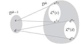
Figure 5. Relation between models $\mathcal{D}^{k-1}$ and $\mathcal{D}^{k}$. Every element in $\mathcal{D}^{k-1}$ is related to a sub-lattice of elements in $\mathcal{D}^{k}$.

Lemma 4.

For every $0<k\leq m$, and every type $A$, we have:

1. $\mathcal{L}^{k}_{A}$ is a lattice: if $(d_{1},d_{2})$, $(e_{1},e_{2})$ are in $\mathcal{L}^{k}_{A}$, then so are $(d_{1}\vee e_{1},d_{2}\vee e_{2})$ and $(d_{1}\land e_{1},d_{2}\land e_{2})$.

2. Given $(d_{1},d_{2})$ and $(e_{1},e_{2})$ in $\mathcal{L}^{k}_{A}$, if $d_{2}\leq e_{2}$ then $d_{1}\leq e_{1}$.

3. Given $d_{2}$ in $\mathcal{D}^{k}_{A}$, there is a unique $d_{1}$ in $\mathcal{D}^{k-1}_{A}$, so that $(d_{1},d_{2})$ in $\mathcal{L}^{k}_{A}$. Let us denote this unique element $d_{2}^{\downarrow}$.

4. If $d_{1}\leq e_{1}$ in $\mathcal{D}^{k-1}_{A}$, then:

   1. there is $e_{1}^{\uparrow_{\lor}}$ in $\mathcal{L}^{k}_{A}(e_{1})$ so that for every $d_{2}$ in $\mathcal{L}^{k}_{A}(d_{1})$ we have $d_{2}\leq e_{1}^{\uparrow_{\lor}}$,

   2. there is $d_{1}^{\uparrow_{\land}}$ in $\mathcal{L}^{k}_{A}(d_{1})$ so that for every $e_{2}$ in $\mathcal{L}^{k}_{A}(e_{1})$ we have $d_{2}^{\uparrow_{\land}}\leq e_{2}$.

Proof 4.1.

Item $0$ can be proved by a straightforward induction on the size of types.

The proof of items $1,2,3$, is by simultaneous induction on the size of $A$. Notice that item $2$ is an immediate consequence of item $1$. We shall therefore not prove it, but we feel free to use it as an induction hypothesis.

We start with the case when $A$ is the base type $o$:

Ad 1. In that case $\mathcal{D}^{k}_{A}=Q_{\leq k}$, $e_{1}=e_{2}\cap Q_{\leq k-1}$ and $d_{1}=d_{2}\cap Q_{\leq k-1}$. Thus, we indeed have that $d_{2}\leq e_{2}$ implies that $d_{1}\leq e_{1}$.

Ad 3. Here, we have $\mathcal{D}^{k-1}_{A}=Q_{\leq k-1}$ and then letting $e_{1}^{\uparrow_{\lor}}=e_{1}\cup Q_{k}$ and $d_{2}^{\uparrow_{\land}}=d_{2}$ is enough to conclude.

Let us now suppose that $A=B\to C$:

Ad 1. Given $f_{1}$ in $\mathcal{D}^{k-1}_{B}$, by induction hypothesis, using item 3, we know that there exist $f_{2}$ in $\mathcal{D}^{k}_{B}$ so that $(f_{1},f_{2})$ is in $\mathcal{L}^{k}_{B}$. Thus, we have $(d_{1}(f_{1}),d_{2}(f_{2}))$ and $(e_{1}(f_{1}),e_{2}(f_{2}))$ in $\mathcal{L}_{k,C}$. With the assumption that $d_{2}\leq e_{2}$, we obtain $d_{2}(f_{2})\leq e_{2}(f_{2})$. By induction hypothesis we get $e_{1}(f_{1})\leq d_{1}(f_{1})$. As $f_{1}$ is arbitrary, we can conclude that $e_{1}\leq d_{1}$.

Ad 3. By induction hypothesis, using item 2, for $f_{2}$ in $\mathcal{D}^{k}_{B}$, there is a unique element $f_{2}^{\downarrow}$ of $\mathcal{D}^{k-1}_{B}$ so that $(f_{2}^{\downarrow},f_{2})$ is in $\mathcal{L}^{k}_{B}$. Given $h_{1}$ in $\mathcal{D}^{k-1}_{A}$ we define for every element $f_{2}$ in $\mathcal{D}^{k}_{B}$:

$$h_{1}^{\uparrow_{\lor}}(f_{2})=(h_{1}(f_{2}^{\downarrow}))^{\uparrow_{\lor}}\qquad h_{1}^{\uparrow_{\land}}(f_{2})=(h_{1}(f_{2}^{\downarrow}))^{\uparrow_{\land}}\ .$$

We will verify only item 3(a), the case of $h_{1}^{\uparrow_{\land}}$ being analogous.

We need to check that $h_{1}^{\uparrow_{\lor}}$ is in $\mathcal{D}^{k}_{A}$. First of all we need to check that it is in $\mathrm{mon}[\mathcal{D}^{k}_{B}\mapsto\mathcal{D}^{k}_{C}]$. Take $g_{2}$ and $f_{2}$ in $\mathcal{D}^{k}_{B}$ so that $g_{2}\leq f_{2}$. By induction hypothesis, using item 1, we have that $g_{2}^{\downarrow}\leq f_{2}^{\downarrow}$. Then $h_{1}(g_{2}^{\downarrow})\leq h_{1}(f_{2}^{\downarrow})$ by monotonicity of $h_{1}$. From item 3 of induction hypothesis we obtain $(h_{1}(g_{2}^{\downarrow}))^{\uparrow_{\lor}}\leq(h_{1}(f_{2}^{\downarrow}))^{\uparrow_{\lor}}$; proving that $h_{1}^{\uparrow_{\lor}}$ is monotone.

Next, we show that $(h_{1},h_{1}^{\uparrow_{\lor}})$ is in $\mathcal{L}^{k}_{A}$. If we take $(f_{2}^{\downarrow},f_{2})$ in $\mathcal{L}_{k,B}$, we obtain by the induction hypothesis, item 3, that $(h_{1}(f_{2}^{\downarrow}),(h_{1}(f_{2}^{\downarrow}))^{\uparrow_{\lor}})$ is in $\mathcal{L}^{k}_{C}$. But, by our definition, this implies that $(h_{1}(f_{2}^{\downarrow}),h_{1}^{\uparrow_{\lor}}(f_{2}))$ is in $\mathcal{L}^{k}_{C}$. As $f_{2}$ is arbitrary we obtain that $(h_{1},h_{1}^{\uparrow_{\lor}})$ is indeed in $\mathcal{L}^{k}_{A}$ proving then that $h_{1}^{\uparrow_{\lor}}$ is in $\mathcal{D}^{k}_{A}$.

It remains to prove that, given $d_{1}\leq e_{1}$ in $\mathcal{D}^{k}_{A}$, for all $d_{2}$ in $\mathcal{L}^{k}_{A}(d_{1})$ we have $d_{2}\leq e_{1}^{\uparrow_{\lor}}$. Given $(f_{2}^{\downarrow},f_{2})$ in $\mathcal{L}^{k}_{B}$, we have $(d_{1}(f_{2}^{\downarrow}),d_{2}(f_{2}))$ in $\mathcal{L}^{k}_{C}$. Using induction hypothesis, item 3, we get $d_{2}(f_{2})\leq(d_{1}(f_{2}^{\downarrow}))^{\uparrow_{\lor}}$. Since $d_{1}\leq e_{1}$ we obtain $d_{2}(f_{2})\leq(e_{1}(f_{2}^{\downarrow}))^{\uparrow_{\lor}}$ that is the desired $d_{2}(f_{2})\leq e_{1}^{\uparrow_{\lor}}(f_{2})$. As $f_{2}$ is arbitrary, this shows that $d_{2}\leq e_{1}^{\uparrow_{\lor}}$.

Notice that the fact that $\mathcal{D}^{k}_{A}$ is a complete lattice is an immediate consequence from the fact that $\mathcal{L}^{k}_{A}$ is a complete lattice.

The formalization of the intuition that $\mathcal{D}^{k}_{A}$ is a refinement of $\mathcal{D}^{k-1}_{A}$ is given by the fact that the mappings $(\cdot)^{\downarrow}$ and $(\cdot)^{\uparrow_{\lor}}$ form a Galois connection between $\mathcal{D}^{k}_{A}$ and $\mathcal{D}^{k-1}_{A}$ and that $(\cdot)^{\downarrow}$ and $(\cdot)^{\uparrow_{\land}}$ form a Galois connection between $\mathcal{D}^{k-1}_{A}$ and $\mathcal{D}^{k}_{A}$.

Corollary 5.

For each $k\leq m$, and each type $A$, $\mathcal{D}^{k}_{A}$ is a non-empty lattice.

The mappings $(\cdot)^{\downarrow}$ and $(\cdot)^{\uparrow_{\lor}}$ form a Galois connection between $\mathcal{D}^{k}_{A}$ and $\mathcal{D}^{k-1}_{A}$. For every $d_{2}\in\mathcal{D}^{k}_{A}$ and $e_{1}\in\mathcal{D}^{k-1}_{A}$ we have: $d_{2}^{\downarrow}\leq e_{1}\quad\text{ iff }\quad d_{2}\leq e_{1}^{\uparrow_{\lor}}$.

Similarly $(\cdot)^{\downarrow}$ and $(\cdot)^{\uparrow_{\land}}$ form a Galois connection between $\mathcal{D}^{k-1}_{A}$ and $\mathcal{D}^{k}_{A}$. For every $d_{1}\in\mathcal{D}^{k-1}_{A}$ and $e_{2}\in\mathcal{D}^{k}_{A}$ we have: $d_{1}^{\uparrow_{\land}}\leq e_{2}\quad\text{ iff }\quad d_{1}\leq e_{2}^{\downarrow}$.

From now on, $\bot^{k}_{A}$ and $\top^{k}_{A}$ will denote the least and the greatest element of $\mathcal{D}^{k}_{A}$.

Corollary 6.

Given $d_{2}$ in $\mathcal{D}^{k}_{B\to C}$ and $e_{2}$ in $\mathcal{D}^{k}_{B}$, we have $(d_{2}(e_{2}))^{\downarrow}=d_{2}^{\downarrow}(e_{2}^{\downarrow})$. Given $d_{1}$ in $\mathcal{D}^{k-1}_{B\to C}$ and $e_{2}$ in $\mathcal{D}^{k}_{B}$, we have: $d_{1}^{\uparrow_{\land}}(e_{2})=(d_{1}(e_{2}^{\downarrow}))^{\uparrow_{\land}}$ and $d_{1}^{\uparrow_{\lor}}(e_{2})=(d_{1}(e_{2}^{\downarrow}))^{\uparrow_{\lor}}$.

Finally, we show one more decomposition property of our models that we will use later to show a correspondence between types and elements of the model (Lemma 20).

We define an operation $\overline{d}$ on the elements $d$ of $\mathcal{D}^{k}_{A}$ by induction on $A$:

• if $A=o$, then $\overline{d}=d\cap Q_{k}$,

• if $A=B\to C$, then for $e$ in $\mathcal{D}^{k}_{B}$, $\overline{d}(e)=\overline{d(e)}$.

A simple induction shows that the operation $\overline{(\cdot)}$ is an involution and that $\overline{\overline{d}}=\overline{d}$. A similar induction shows that $\overline{(\cdot)}$ is the identity function on $\mathcal{L}^{k}_{A}(\bot^{k-1}_{A})$.

Lemma 7.

For every $0<k\leq m$, and every $d$ in $\mathcal{D}^{k}_{A}$; let $\overline{d}$ be as defined above, and let $\widetilde{d}=(\top^{k-1}_{A})^{\uparrow_{\land}}\vee\overline{d}$. We have $d=((d^{\downarrow})^{\uparrow_{\land}})\vee\overline{d}$ and $d=((d^{\downarrow})^{\uparrow_{\lor}})\wedge\widetilde{d}$.

Proof 4.2.

We prove only the first identity, the second being similar. The proof is by induction on the size of $A$.

In case $A=o$, from definitions we get $\overline{d}=d\cap Q_{k}$ while $(d^{\downarrow})^{\uparrow_{\land}}=d\cap Q_{\leq k-1}$. Thus we indeed have $d=((d^{\downarrow})^{\uparrow_{\land}})\vee\overline{d}$.

In case $A=B\to C$. Given $e$ in $\mathcal{D}^{k}_{B}$, we have that $(d^{\downarrow})^{\uparrow_{\land}}(e)=(d^{\downarrow}(e^{\downarrow}))^{\uparrow_{\land}}=((d(e))^{\downarrow})^{\uparrow_{\land}}$. Moreover, $\overline{d}(e)=\overline{d(e)}$. Therefore, $(((d^{\downarrow})^{\uparrow_{\land}})\vee\overline{d})(e)=(((d(e))^{\downarrow})^{\uparrow_{\land}})\vee\overline{d(e)}$. But, by induction, we have $d(e)=(((d(e))^{\downarrow})^{\uparrow_{\land}})\vee\overline{d(e)}=(((d^{\downarrow})^{\uparrow_{\land}})\vee\overline{d})(e)$. As $e$ is arbitrary, we get the identity.

Lemma 8.

Given $e_{1}$, $e_{2}$ in $\mathcal{D}^{k}_{A}$ and $d$ in $\mathcal{D}^{k-1}_{A}$:

• if $\overline{e_{1}}\neq\overline{e_{2}}$ then $d^{\uparrow_{\land}}\vee\overline{e_{1}}\neq d^{\uparrow_{\land}}\vee\overline{e_{2}}$,

• if $\widetilde{e_{1}}\neq\widetilde{e_{2}}$ then $d^{\uparrow_{\lor}}\wedge\overline{e_{1}}\neq d^{\uparrow_{\lor}}\wedge\overline{e_{2}}$,

Proof 4.3.

We only prove the first identity, the second being essentially dual.

We proceed by induction on $A$. When $A=o$, then as $d^{\uparrow_{\land}}=d$ (see the proof of Lemma 4), $d\subseteq Q_{\leq k-1}$ and $\overline{e_{1}}$, $\overline{e_{2}}$ are included in $Q_{k}$, the conclusion is immediate.

When $A=B\to C$, since $\overline{e_{1}}\neq\overline{e_{2}}$ there is $a$ so that $\overline{e_{1}}(a)\neq\overline{e_{2}}(a)$. Now we have $(d^{\uparrow_{\land}}\vee\overline{e_{i}})(a)=d^{\uparrow_{\land}}(a)\vee\overline{e_{i}}(a)=(d(a^{\downarrow}))^{\uparrow_{\land}}\vee\overline{e_{i}(a)}$ for $i$ in $\{1,2\}$. The induction hypothesis implies that $(d(a^{\downarrow}))^{\uparrow_{\land}}\vee\overline{e_{1}(a)}\neq(d(a^{\downarrow}))^{\uparrow_{\land}}\vee\overline{e_{2}(a)}$. Therefore $(d^{\uparrow_{\land}}\vee\overline{e_{1}})(a)\neq(d^{\uparrow_{\land}}\vee\overline{e_{2}})(a)$ and $d^{\uparrow_{\land}}\vee\overline{e_{1}}\neq d^{\uparrow_{\land}}\vee\overline{e_{2}}$ as desired.

Lemma 7 shows that every element $d_{2}$ in $\mathcal{L}^{k}_{A}(d_{1})$ is of the form $d_{1}^{\uparrow_{\land}}\vee e_{2}$ with $e_{2}$ in $\mathcal{L}^{k}_{A}(\bot^{k-1}_{A})$ and of the form $d_{1}^{\uparrow_{\lor}}\wedge e_{2}$ with $e_{2}$ in $\mathcal{L}^{k}_{A}(\top^{k-1}_{A})$. Thus not only $\mathcal{L}^{k}_{A}$ puts every element $d_{1}$ in relation with a lattice $\mathcal{L}^{k}(d_{1})$, but, from Lemma 8, this relation is injective. As a consequence the lattice $\mathcal{L}^{k}_{A}(d_{1})$ is isomorphic to $\mathcal{L}^{k}_{A}(\bot^{k-1}_{A})$ and to $\mathcal{L}^{k}_{A}(\top^{k-1}_{A})$, showing as we said earlier, that for any $e$ and $d$ in $\mathcal{D}^{k-1}_{A}$, $\mathcal{L}^{k}_{A}(e)$ is isomorphic to $\mathcal{L}^{k}_{A}(d)$. Another consequence is that $\mathcal{D}^{k}_{A}$ is isomorphic to the lattice $\mathcal{D}^{k-1}_{A}\times\mathcal{L}_{k,A}(\bot^{k-1}_{A})$ or to the lattice $\mathcal{D}^{k-1}_{A}\times\mathcal{L}_{k,A}(\top^{k-1}_{A})$. This isomorphism is important as it shows that the types we have described Section 3 are a faithful representation of the elements of the model we have just constructed.

4.2. Fixpoints in a stratified model

The properties from the previous subsection allow us to define fixpoint operators in every applicative structure $\mathcal{D}^{k}$. Then we can show that a stratified structure is a model of $\lambda Y$-calculus.

For $f\in\mathcal{D}^{0}_{A\to A}$ we define $\mathrm{fix}^{0}_{A}(f)=\bigwedge\{f^{n}(\top^{0}):n\geq 0\}$. For $0<2k\leq m$ and $f\in\mathcal{D}^{2k}_{A\to A}$ we define

$$\mathrm{fix}^{2k}_{A}(f)=\bigwedge\{f^{n}(e):n\geq 0\}\text{ where }e=(\mathrm{fix}^{2k-1}_{A}(f^{\downarrow}))^{\uparrow_{\lor}}$$

For $0<2k+1\leq m$ and $f\in\mathcal{D}^{2k+1}_{A\to A}$ we define

$$\mathrm{fix}^{2k+1}_{A}(f)=\bigvee\{f^{n}(d):n\geq 0\}\text{ where }d=(\mathrm{fix}^{2k}_{A}(f^{\downarrow}))^{\uparrow_{\land}}$$

Observe that, for even $k$, $e$ is obtained with $(\cdot)^{\uparrow_{\lor}}$; while for odd $k$, $(\cdot)^{\uparrow_{\land}}$ is used.

The intuitive idea behind the definition of the fixpoint is presented in Figure 6. On stratum $0$ it is just the greatest fixpoint. Then this greatest fixpoint, call it $d$, is lifted to stratum $1$, and the least fixpoint computation is started in the complete sub-lattice of the refinements of $d$. The result is then lifted to stratum $2$, and once again the greatest fixpoint computation is started, and so on. The Galois connections between strata guarantee that this process makes sense.

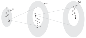
Figure 6. A computation of a fixpoint: it starts in $\mathcal{D}^{0}$, and then the least and the greatest fixpoints alternate.

It remains to show that equipped with the interpretation of fixpoints given by Definition 4.2 the applicative structure $\mathcal{D}^{k}$ is a model of the $\lambda Y$-calculus. First, we check that $\mathrm{fix}^{k}_{A}$ is indeed an element of the model and that it is a fixpoint.

Lemma 9.

For every $0\leq k\leq m$ and every type $A$ we have that $\mathrm{fix}^{k}_{A}$ is monotone, and if $k>0$ then $(\mathrm{fix}^{k-1}_{A},\mathrm{fix}^{k}_{A})\in\mathcal{L}^{k}_{(A\to A)\to A}$. Moreover for every $f$ in $\mathcal{D}^{k}_{A\to A}$, $f(\mathrm{fix}^{k}_{A}(f))=\mathrm{fix}^{k}_{A}(f)$.

Proof 4.4.

We proceed by induction on $k$. For $0$ the statement is obvious. We will only consider the case where $k$ is even, the other being dual.

Consider the case $2k>0$. First we show monotonicity. Suppose $g\leq h$ are two elements of $\mathcal{D}^{2k}_{A\to A}$. By Lemma 4 we get $g^{\downarrow}\leq h^{\downarrow}$. Consider $g^{1}=\mathrm{fix}^{2k-1}_{A}(g^{\downarrow})$ and $h^{1}=\mathrm{fix}^{2k-1}_{A}(h^{\downarrow})$. By induction hypothesis $\mathrm{fix}^{2k-1}_{A}$ is monotone, so $g^{1}\leq h^{1}$. Then, once again using the Lemma 4, we have $(g^{1})^{\uparrow_{\lor}}\leq(h^{1})^{\uparrow_{\lor}}$. This implies $\mathrm{fix}^{2k}_{A}(g)\leq\mathrm{fix}^{2k}_{A}(h)$.

Now we show $(\mathrm{fix}^{2k-1}_{A},\mathrm{fix}^{2k}_{A})\in\mathcal{L}^{2k}_{(A\to A)\to A}$. We take an arbitrary pair $(f_{1},f_{2})\in\mathcal{L}^{2k}_{A\to A}$ and we need to show that $(\mathrm{fix}^{2k-1}_{A}(f_{1}),\mathrm{fix}^{2k}_{A}(f_{2}))\in\mathcal{L}^{2k}_{A}$. This follows from the following calculation

$$(\mathrm{fix}^{2k-1}(f_{1}),(\mathrm{fix}^{2k-1}(f_{1}))^{\uparrow_{\lor}})\in \mathcal{L}^{2k}_{A}\quad\text{ by Lemma~{}\ref{lem:galloi_connections}}$$

$$(f_{1}(\mathrm{fix}^{2k-1}(f_{1})),f_{2}((\mathrm{fix}^{2k-1}(f_{1})^{\uparrow_{\lor}}))\in \mathcal{L}^{2k}_{A}\quad\text{by logical relation}$$

$$(\mathrm{fix}^{2k-1}(f_{1}),f_{2}((\mathrm{fix}^{2k-1}(f_{1})^{\uparrow_{\lor}}))\in \mathcal{L}^{2k}_{A}\quad\text{since $\mathrm{fix}^{2k-1}(f_{1})$ }$$

 is a fixpoint of $$f_{1}$$

$$(\mathrm{fix}^{2k-1}(f_{1}),f^{i}_{2}((\mathrm{fix}^{2k-1}(f_{1})^{\uparrow_{\lor}}))\in \mathcal{L}^{2k}_{A}\quad\text{for every $i\geq 0$}$$

Moreover, from Lemma 4, we have that $f_{2}((\mathrm{fix}^{2k-1}(f_{1})^{\uparrow_{\lor}})\leq(\mathrm{fix}^{2k-1}(f_{1}))^{\uparrow_{\lor}}$. This implies

$$f_{2}^{i+1}((\mathrm{fix}^{2k-1}(f_{1})^{\uparrow_{\lor}})\leq f_{2}^{i}((\mathrm{fix}^{2k-1}(f_{1}))^{\uparrow_{\lor}})$$

for every $i\in\mathbb{N}$. Therefore, $(f_{2}^{i}((\mathrm{fix}^{2k-1}(f_{1}))^{\uparrow_{\lor}})_{i\in\mathbb{N}}$ is a decreasing sequence of $\mathcal{D}^{2k}_{A}$. Since the model is finite this sequence reaches the fixpoint, namely $\mathrm{fix}^{2k}_{A}(f_{2})=f^{i}_{2}((\mathrm{fix}^{2k-1}_{A}(f_{1})^{\uparrow_{\lor}}))$ for some $i$. Thus, at the same time, this shows that $(\mathrm{fix}^{2k-1}_{A}(f_{1}),\mathrm{fix}^{2k}_{A}(f_{2}))\in\mathcal{L}^{2k}_{A}$ and that $\mathrm{fix}^{2k}(f_{2})$ is a fixpoint of $f_{2}$.

This lemma has the following interesting corollary that will prove useful in the study of type systems.

Corollary 10.

For $k>0$, $A$ a type, and $f\in\mathcal{D}^{k}_{A\to A}$ we have

$$\mathrm{fix}^{2k}_{A}(f)= \bigvee\{d\mid f(d)\geq d\text{ and }d^{\downarrow}=\mathrm{fix}^{2k-1}_{A}(f)\}$$

$$\mathrm{fix}^{2k+1}_{A}(f)= \bigwedge\{d\mid f(d)\leq d\text{ and }d^{\downarrow}=\mathrm{fix}^{2k}_{A}(f)\}$$

Moreover, the fundamental lemma on logical relations gives us the following consequence.

Corollary 11.

For every $k>0$, every term $M$ and valuation $\nu$ into $\mathcal{D}^{k-1}$ we have $({[\![M]\!]}^{k-1}_{\nu},{[\![M]\!]}^{k}_{\nu^{\uparrow_{\land}}})\in\mathcal{L}^{k}$ and $({[\![M]\!]}^{k-1}_{\nu},{[\![M]\!]}^{k}_{\nu^{\uparrow_{\lor}}})\in\mathcal{L}^{k}$; where $\nu^{\uparrow_{\land}}$ and $\nu^{\uparrow_{\lor}}$ are as expected, i.e. $\nu^{{}^{\uparrow_{\land}}}(x)=(\nu(x))^{{}^{\uparrow_{\land}}}$ and $\nu^{{}^{\uparrow_{\lor}}}(x)=(\nu(x))^{{}^{\uparrow_{\lor}}}$.

Now we turn to showing that for every $k$, $\mathcal{D}^{k}$ is indeed a model of $\lambda Y$-calculus. Since $\mathcal{D}^{k}_{A\to B}$ does not contain all the functions from $\mathcal{D}^{k}_{A}$ to $\mathcal{D}^{k}_{B}$ we must show that there are enough of them to form a model of $\lambda Y$, the main problem being to show that ${[\![\lambda x.M]\!]}_{\upsilon}^{\mathcal{D}^{k}}$ defines an element of $\mathcal{D}^{k}$. For this it will be more appropriate to consider the semantics of a term as a function of values of its free variables. Given a finite sequence of variables $\vec{x}=x_{1},\dots,x_{n}$ of types $A_{1},\dots,A_{n}$ respectively and a term $M$ of type $B$ with free variables in $\vec{x}$, the meaning of $M$ in the model $\mathcal{D}^{k}$ with respect to $\vec{x}$ will be a function ${[\![M]\!]}^{k}_{\vec{x}}$ in $\mathcal{D}^{k}_{A_{1}}\to\dots\to\mathcal{D}^{k}_{A_{n}}\to\mathcal{D}^{k}_{B}$ that represents the function $\lambda\vec{p}.{[\![M]\!]}_{[p_{1}/x_{1},\dots,p_{n}/x_{n}]}^{k}$. Formally it is defined as follows:

1. ${[\![Y^{B}]\!]}_{\vec{x}}^{k}=\lambda\vec{p}.\ \mathrm{fix}_{B}$

2. ${[\![a]\!]}_{\vec{x}}^{k}=\lambda\vec{p}.\ \rho(a)$

3. ${[\![x_{i}^{A_{i}}]\!]}_{\vec{x}}^{k}=\lambda\vec{p}.p_{i}$

4. ${[\![MN]\!]}_{\vec{x}}^{k}=\lambda\vec{p}.\ ({[\![M]\!]}_{\vec{x}}^{k}\,\vec{p})({[\![N]\!]}_{\vec{x}}^{k}\,\vec{p})$

5. ${[\![\lambda y.M]\!]}_{\vec{x}}^{k}=\lambda\vec{p}.\lambda p_{y}.\ {[\![M]\!]}_{\vec{x}y}^{k}\vec{p}p_{y}$

Note that the $\lambda$ symbol on the right hand side of the equality is the semantic symbol used to denote a relevant function, and not a part of the syntax while the sequence $\vec{p}$ denote a sequence of parameters $p_{1}$, …, $p_{n}$ ranging respectively in $\mathcal{D}^{k}_{A_{1}}$, …, $\mathcal{D}^{k}_{A_{n}}$.

Lemma 9 ensures the existence of the meaning of $Y$ in $\mathcal{D}^{k}$. With this at hand, the next lemma provides all the other facts necessary to show that the meaning of a term with respect to $\vec{x}$ is always an element of the model.

Lemma 12.

For every sequence of types $\vec{A}=A_{1}\ldots A_{n}$ and every types $B$, $C$ we have the following:

• For every constant $p\in\mathcal{D}^{k}_{B}$ the constant function $f_{p}:A_{1}\to\dots\to A_{n}\to B$ belongs to $\mathcal{D}^{k}_{A_{1}\to\dots\to A_{n}\to B}$.

• For $i=1,\dots,n$, the projection $\pi_{i}:A_{1}\to\dots\to A_{n}\to A_{i}$ belongs to $\mathcal{D}^{k}_{A_{1}\to\dots\to A_{n}\to B}$.

• If $f:\vec{A}\to(B\to C)$ and $g:\vec{A}\to B$ are in $\mathcal{D}^{k}$ then $\lambda\vec{p}.f\vec{p}(g\vec{p}):\vec{A}\to C$ is in $\mathcal{D}^{k}$.

Proof 4.5.

For the first item we take $p\in\mathcal{D}^{k}_{B}$ and show that the constant function $f_{p}:A\to B$ belongs to $\mathcal{D}^{k}_{A\to B}$. For $k=0$ this is clear. For $k>0$ we take $p^{\downarrow}$ and consider the constant function $f_{p^{\downarrow}}\in\mathcal{D}^{k-1}_{p}$. We have $(f_{p^{\downarrow}},f_{p})\in\mathcal{L}^{k}_{A\to B}$ since $(p^{\downarrow},p)\in\mathcal{L}^{k}_{B}$ by Lemma 4. So $f_{p}\in\mathcal{D}^{k}_{A\to B}$.

The (easy) proofs for the second and the third items follow the same kind of reasoning.

These observations allow us to conclude that $\mathcal{D}^{k}$ is indeed a model of the $\lambda Y$-calculus, that is:

1. for every term $M$ of type $A$ and every valuation $\nu$ ranging of the free variables of $M$, ${[\![M]\!]}_{\nu}^{k}$ is in $\mathcal{D}^{k}_{A}$,

2. given two terms $M$ and $N$ of type $A$, if $M=_{\beta\delta}N$, then for every valuation $\nu$, ${[\![M]\!]}^{k}_{\nu}={[\![N]\!]}^{k}_{\nu}$.

Theorem 13.

For every finite set $Q$, and function $\rho:Q\to\mathbb{N}$. For every $k\leq 0$ the applicative structure $\mathcal{D}^{k}$ is a model of the $\lambda Y$-calculus.

4.3. Correctness and completeness of the model

We show that the models introduced above are expressive enough to recognize all properties definable by weak alternating automata. For a given automaton we will take a model as defined above, and show that with the right interpretation of constants the model can recognize the set of terms whose Böhm trees are accepted by the automaton (Theorem 14).

For the whole section we fix a weak alternating automaton

$$\mathcal{A}=\langle Q,\Sigma,q^{0},\delta_{o},\delta_{o^{2}\to o},\rho\rangle\ ,$$

where $Q$ is a set of states, $\Sigma$ is the alphabet, $\delta_{o}\subseteq Q\times\Sigma$ and $\delta_{o^{2}\to o}:Q\times\Sigma\to\mathcal{P}(\mathcal{P}(Q)\times\mathcal{P}(Q))$ are transition functions, and $\rho:Q\to\mathbb{N}$ is a ranking function. For sake of the simplicity of the notation in this section we assume that the only constants in the signature are either of type $o$ or $o^{2}\to o$.

Recall that weak means that the states in a transition for a state $q$ have ranks at most $\rho(q)$, in other words, for every $(S_{0},S_{1})\in\delta(q,a)$, $S_{0},S_{1}\subseteq Q_{\leq\rho(q)}$. As noted before, without a loss of generality, we assume that $\delta$ is monotone, i.e. if $(S_{0},S_{1})\in\delta(q,a)$ and $S_{0}\subseteq S^{\prime}_{0}\subseteq Q_{\leq\rho(q)}$ and $S_{1}\subseteq S^{\prime}_{1}\subseteq Q_{\leq\rho(q)}$ then $(S^{\prime}_{0},S^{\prime}_{q})\in\delta(q,a)$. For a closed term $M$ of type $o$, let

$$\mathcal{A}(M)=\{q\in Q:\text{$\mathcal{A}$ accepts $BT(M)$ from $q$}\}$$

be the set of states from which $\mathcal{A}$ accepts the tree $BT(M)$.

We want to show that our model $\mathcal{D}^{m}$ as defined in the previous section can calculate $\mathcal{A}(M)$; here $m$ is the maximal value of the rank function of $\mathcal{A}$. The following theorem states a slightly more general fact. Before proceeding we need to fix the meaning of constants:

$${[\![c]\!]}^{k}= \{q\in Q_{\leq k}:(c,q)\in\delta_{o}\}$$

$${[\![a]\!]}^{k}(S_{0},S_{1})= \{q\in Q_{\leq k}:(S_{0},S_{1})\in\delta_{o^{2}\to o}(q,a)\}$$

Notice that, by our assumption about monotonicity of $\delta$, these functions are monotone.

Theorem 14.

For every closed term $M$ of type $o$, and for every $0\leq k\leq m$ we have: ${[\![M]\!]}^{k}=\mathcal{A}(M)\cap Q_{\leq k}$.

The rest of this section is devoted to the proof of the theorem. For $k=0$ the model $\mathcal{D}^{0}$ is just the GFP model over $Q_{0}$. Moreover $\mathcal{A}$ restricted to the states in $Q_{0}$ is an automaton with trivial acceptance conditions. The theorem follows from Theorem 1.

For the induction step consider an even $k>0$. The case where $k$ is odd is similar and we will not present it here. The two directions of Theorem 14 are proved using different techniques. The next lemma shows the left to right inclusion and is based on a rather simple unrolling. The other inclusion is proved using a logical relation between the syntactic model of the $\lambda Y$-calculus and the stratified model (Lemma 18). This relation allows us to formally relate the abstractions built into the model to their syntactic meanings that are expressed by the acceptance of Böhm trees of closed $\lambda Y$-terms of atomic type by the weak parity automaton.

Lemma 15.

${[\![M]\!]}^{k}\subseteq\mathcal{A}(M)$.

Proof 4.6.

We take $q\in{[\![M]\!]}^{k}$ and describe a winning strategy for $Eve$ in the acceptance game of $\mathcal{A}$ on $BT(M)$ from $q$ (cf. page 2). If the rank of $q<k$ then such a strategy exists by the induction assumption. So we suppose that $\rho(q)=k.$

If $M$ does not have a head normal form then $BT(M)$ consists just of the root $\varepsilon$ labeled with $\Omega$. Then Eve wins by the definition of the game since $k$ is even.

If the head normal form of $M$ is a constant $c:o$ then since $q\in{[\![c]\!]}^{k}$ we have $(q,c)\in\delta_{o}$. Eve wins by the definition of the game.

Suppose then that $M$ has a head normal form $aM_{0}M_{1}$. As ${[\![M]\!]}^{k}={[\![aM_{0}M_{1}]\!]}^{k}$ we have $q\in{[\![aM_{0}M_{1}]\!]}^{k}$. By the semantics of $a$ we know that $({[\![M_{0}]\!]}^{k},{[\![M_{1}]\!]}^{k})\in\delta(q,a)$. The strategy of Eve is to choose $({[\![M_{0}]\!]}^{k},{[\![M_{1}]\!]}^{k})$. Suppose Adam then selects $i\in\{0,1\}$ and $q_{i}\in{[\![M_{i}]\!]}^{k}$. If $\rho(q_{i})<k$ then Eve has a winning strategy by induction hypothesis. Otherwise, if $\rho(q_{i})=k$ we repeat the reasoning.

This strategy is winning for Eve since a play either stays in states of even rank $k$ or switches to a play following a winning strategy for smaller ranks.

It remains to show that $\mathcal{A}(M)\cap Q_{\leq k}\subseteq{[\![M]\!]}^{k}$. For this we will define one logical relation between $\mathcal{D}^{k}$ and the syntactic model of $\lambda Y$ and show a couple of lemmas.

We define a logical relation between the model $\mathcal{D}^{k}$ and closed terms

$$R^{k}_{0}= \{(P,M):\mathcal{A}(M)\cap Q_{\leq k}\subseteq P\}$$

$$R^{k}_{A\to B}= \{(f,M):\forall_{(g,N)\in R_{A}}.\ (f(g),MN)\in R_{B}\}\ .$$

Since $R^{k}$ is a logical relation we have:

Lemma 16.

If $M=_{\beta\delta}N$ and $(f,M)\in R^{k}_{A}$ then $(f,N)\in R^{k}_{A}$.

The next lemma shows a relation between $R^{k}$ and $R^{k-1}$.

Lemma 17.

For every type $A$, $f\in\mathcal{D}^{k}_{A}$, $g\in\mathcal{D}^{k-1}_{A}$:

• if $(f,M)\in R^{k}_{A}$ then $(f^{\downarrow},M)\in R^{k-1}_{A}$;

• if $(g,M)\in R^{k-1}_{A}$ then $(g^{\uparrow_{\lor}},M)\in R^{k}$;

Proof 4.7.

The proof is an induction on the size of the type. The base case is when $A=o$.

For the first item suppose $(f,M)\in R^{k}_{A}$. By definition, this means $\mathcal{A}(M)\cap Q_{\leq k}\subseteq f$. Then $\mathcal{A}(M)\cap Q_{\leq k-1}\subseteq f\cap Q_{\leq k-1}=f^{\downarrow}$. So $(f^{\downarrow},M)\in R^{k-1}_{A}$.

For the second item suppose $(g,M)\in R^{k-1}_{A}$. So $\mathcal{A}(M)\cap Q_{\leq k-1}\subseteq g$. We have $\mathcal{A}(M)\cap Q_{\leq k}\subseteq(\mathcal{A}(M)\cap Q_{\leq k-1})\cup Q_{k}\subseteq g\cup Q_{k}=g^{\uparrow_{\lor}}$.

For the induction step let $A$ be $B\to C$. Let us consider the first item. Suppose $(f,M)\in R^{k}_{B\to C}$. Take $(h,N)\in R^{k-1}_{B}$, we need to show that $(f^{\downarrow}(h),MN)\in R^{k-1}_{C}$. By the second item of the induction hypothesis we get $(h^{\uparrow_{\lor}},N)\in R^{k}_{B}$. Then $(f(h^{\uparrow_{\lor}}),MN)\in R^{k}_{C}$, by the definition of $R^{k}_{B\to C}$. Using the first item of the induction hypothesis we get $((f(h^{\uparrow_{\lor}}))^{\downarrow},MN)\in R^{k-1}_{C}$. Then using Corollaries 5 and 6 we obtain $(f(h^{\uparrow_{\lor}}))^{\downarrow}=f^{\downarrow}((h^{\uparrow_{\lor}})^{\downarrow})=f^{\downarrow}(h)$.

For the proof of the second item consider $(g,M)\in R^{k-1}_{B\to C}$ and $(h,N)\in R^{k}_{B}$. We need to show that $(g^{\uparrow_{\lor}}(h),MN)\in R^{k}_{C}$. From the first item of the induction hypothesis we obtain $(h^{\downarrow},N)\in R^{k-1}_{B}$, so $(g(h^{\downarrow}),MN)\in R^{k-1}_{C}$. The second item of the induction hypothesis gives us $((g(h^{\downarrow}))^{\uparrow_{\lor}},MN)\in R^{k}_{C}$. We are done since $g^{\uparrow_{\lor}}(h)=(g(h^{\downarrow}))^{\uparrow_{\lor}}$ by Corollary 6.

The right to left inclusion of Theorem 14 is implied by the following more general statement.

Lemma 18.

Let $v$ be a valuation, and let $\sigma$ be a substitution of closed terms satisfying $(v(x^{A}),\sigma(x^{A}))\in R^{k}_{A}$ for every variable $x^{A}$ in the domain of $\sigma$. For every term $M$ of a type $A$ we have $({[\![M]\!]}^{k}_{v},M.\sigma)\in R^{k}_{A}$.

Proof 4.8.

The proof is by induction on the structure of $M$.

If $M$ is a variable then the proof is immediate.

If $M$ is a constant $a$ then we show that $({[\![a]\!]},a)\in R^{k}_{o\to o\to o}$. For this we take arbitrary $(S_{0},N_{0}),(S_{1},N_{1})\in R^{k}_{0}$, and we show that $({[\![a]\!]}^{k}(S_{0},S_{1}),aN_{0}N_{1})\in R^{k}_{0}$. Take $q\in\mathcal{A}(aN_{0}N_{1})\cap Q_{\leq k}$. Let us look at Eve’s winning strategy in the acceptance game from $q$ on $BT(aN_{0}N_{1})$. In the first round of this game she chooses some $(T_{0},T_{1})\in\delta(a,q)$. So $q\in{[\![a]\!]}(T_{0},T_{1})$. Since her strategy is winning we have $T_{0}\subseteq\mathcal{A}(N_{0})$ and $T_{1}\subseteq\mathcal{A}(N_{1})$, and by weakness of the automaton $T_{0},T_{1}\subseteq Q_{\leq k}$. From the definition of $R^{k}_{0}$ we get $\mathcal{A}(N_{0})\cap Q_{\leq k}\subseteq S_{0}$ and $\mathcal{A}(N_{1})\cap Q_{\leq k}\subseteq S_{1}$. By monotonicity we get the desired $q\in{[\![a]\!]}(S_{0},S_{1})$.

If $M$ is an application $NP$ then the conclusion is immediate from the definition of $R^{k}_{A}$ and the induction hypothesis.

If $M$ is an abstraction $\lambda x.\ N:B\to C$, then we take $(g,P)\in R^{k}_{B}$. By induction hypothesis $({[\![N]\!]}^{k}_{v[g/x]},N.\sigma[P/x])\in R^{k}_{C}$. So $({[\![M]\!]}^{k}_{v}(g),MP)\in R^{k}_{C}$ by Lemma 16.

If $M=Y^{(A\to A)\to A}$. Take $(f,P)\in R^{k}_{A\to A}$. By Lemma 17 we have $(f^{\downarrow},P)\in R^{k-1}_{A\to A}$. As by the outermost induction hypothesis

$$(\mathrm{fix}_{A}^{k-1},Y^{(A\to A)\to A})\in R^{k-1}_{(A\to A)\to A}\ ,$$

and we obtain $(\mathrm{fix}^{k-1}_{A}(f^{\downarrow}),YP)\in R^{k-1}_{A}$. Once again using Lemma 17 we can deduce $((\mathrm{fix}^{k-1}_{A}(f^{\downarrow}))^{\uparrow_{\lor}},YP)\in R^{k}_{A}$. By the choice of $(f,P)$ we obtain

$$(f((\mathrm{fix}^{k-1}_{A}(f^{\downarrow}))^{\uparrow_{\lor}}),P(YP))\in R^{k}_{A}\ .$$

Since $YP=_{\beta\delta}P(YP)$, we have $(f^{i}((\mathrm{fix}^{k-1}_{A}(f^{\downarrow}))^{\uparrow_{\lor}}),YP)\in R^{k}_{A}$ for all $i\geq 0$. Since the sequence of $f^{i}((\mathrm{fix}^{k-1}_{A}(f^{\downarrow}))^{\uparrow_{\lor}})$ is decreasing, it reaches the fixpoint $\mathrm{fix}^{k}_{A}(f)$ in a finite number of steps and $(\mathrm{fix}^{k}_{A}(f),YP)$ is in $R_{A}$. As $(f,P)$ is an arbitrary element of $R^{k}_{A\to A}$, this shows that $(\mathrm{fix}^{k}_{A},Y)$ is in $R^{k}_{(A\to A)\to A}$.

5. From models to type systems

We are now in a position to show that our type system from Figure 3 can reason about the values of $\lambda Y$-terms in a stratified model, cf. Theorem 23 below. Thanks to Theorem 14 this means that the type system can talk about the acceptance of the Böhm tree of a term by the automaton. This implies the soundness and completeness of our type system, Theorem 2.

Throughout this section we work with a fixed signature $\Sigma$ and a fixed weak alternating automaton $\mathcal{A}=\langle Q,\Sigma,q^{0},\delta_{o},\delta_{o^{2}\to o},\rho\rangle$. As in the previous section, for the sake of the simplicity of notations we will assume that the constants in the signature are of type $o$ or $o\to o\to o$. We will also prefer the notation $Yx.M$ to $Y(\lambda x.M)$.

The arrow constructor in types will be interpreted as a step function in the model. Step functions are particular monotone functions from a lattice $\mathcal{L}_{1}$ to a lattice $\mathcal{L}_{2}$. For later use we also define co-step functions. For $d$ in $\mathcal{L}_{1}$ and $e$ in $\mathcal{L}_{2}$, the step function $d$ and the co-step function $d\rightharpoonup g$ are defined by:

$$(d \left\{\begin{array}[]{l}e\text{ when }d\leq h\\ \bot\text{ otherwise}\end{array}\right. (d\rightharpoonup e)(h)= \left\{\begin{array}[]{l}e\text{ when }h\leq d\\ \top\text{ otherwise\ .}\end{array}\right.$$

To emphasize that we work in $\mathcal{D}^{k}$ we will sometimes write $d$ and $d\rightharpoonup^{k}e$.

Types introduced on page 3 can be meaningfully interpreted at every level of the model. So ${[\![t]\!]}^{k}$ will denote the interpretation of $t$ in $\mathcal{D}^{k}$ defined as follows.

$${[\![q]\!]}^{k} =\{q\}\text{ if }\rho(q)\leq k,\,\emptyset\text{ otherwise}$$

$${[\![S]\!]}^{k} =\bigvee\{{[\![t]\!]}^{k}:t\in S\}\qquad\text{for $S\subseteq\mathrm{Types}_{A}$}$$

$${[\![T\to s]\!]}^{k} ={[\![T]\!]}^{k}$$

Directly from the definition we have ${[\![S_{1}\cup S_{2}]\!]}^{k}={[\![S_{1}]\!]}^{k}\vee{[\![S_{2}]\!]}^{k}$, and ${[\![S\to T]\!]}^{k}={[\![S]\!]}^{k}$.

The next lemma summarizes basic facts about the interpretation of types. Recall that the application operation $S(T)$ on types (cf. page 3) means $\{t:(U\to t)\in S\land U\sqsubseteq T\}$. The proof of the lemma uses Corollaries 6 and 5.

Lemma 19.

For every type $A$, if $S\subseteq\mathrm{Types}_{A}$ and $k\leq m$ we have: ${[\![S]\!]}^{k}={[\![S\cap\mathrm{Types}^{k}_{A}]\!]}^{k}$, ${[\![S\cap\mathrm{Types}^{k}_{A}]\!]}^{k+1}=({[\![S]\!]}^{k}_{A})^{\uparrow_{\land}}$ and ${[\![S]\!]}^{k}=({[\![S]\!]}^{k+1})^{\downarrow}$.

Proof 5.6.

Consider the first statement. Since ${[\![S]\!]}^{k}=\bigvee\{{[\![t]\!]}^{k}:t\in S\}$ it is sufficient to show that ${[\![t]\!]}^{k}=\bot^{k}_{A}$ for $t\not\in\mathrm{Types}^{k}_{A}$. We do it by induction on the type $A$.

Suppose that $t\in\mathrm{types}^{l}_{A}$ for $l>k$. For the type $o$ it follows directly from the definition that ${[\![t]\!]}^{k}=\emptyset$. For $A$ of the form $B\to C$ we know that $t$ is of the form $T\to s$ with $T\subseteq\mathrm{Types}^{l}_{B}$ and $s\in\mathrm{types}^{l}_{C}$. By induction assumption ${[\![s]\!]}^{k}=\bot^{k}_{C}$. We get ${[\![T\to s]\!]}^{k}={[\![T]\!]}^{k}$.

We give the proof of the second statement, the proof of the third is analogous. We prove the result only for elements of $\mathrm{types}^{k}_{A}$ as the more general one is a direct consequence of that particular case. The proof is by induction on $A$. The base case is obvious. For $A$ of the form $B\to C$ we have ${[\![T\to s]\!]}^{k+1}$ is by definition ${[\![T]\!]}^{k+1}$ which by induction hypothesis is $({[\![T]\!]}^{k})^{\uparrow_{\land}}$. We will be done if we show that for every $f\in\mathcal{D}^{k}_{B}$ and $g\in\mathcal{D}^{k}_{C}$:

$$f^{\uparrow_{\land}}$$ Step 5.11

Given $e$ in $\mathcal{D}^{k+1}_{B}$, by Corollary 6, we have $(f$ is equal to $((f$, and therefore:

$$(f$$ Step 5.15

Since $f\leq e^{\downarrow}$ iff $f^{\uparrow_{\land}}\leq e$, by Corollary 5, this proves the desired equality.

Actually every element of $\mathcal{D}^{k}$ is the image of some type via ${[\![\cdot]\!]}^{k}$: types are syntactic representations of the model. For this we use $\overline{(\cdot)}$ operation (cf. Definition 4.1).

Lemma 20.

For every $k\leq m$, every type $A$ and every $d$ in $\mathcal{D}^{k}_{A}$ there is $S\subseteq\mathrm{Types}^{k}_{A}$ so that ${[\![S]\!]}^{k}=d$, and there is $S^{\prime}\subseteq\mathrm{types}^{k}_{A}$ so that ${[\![S^{\prime}]\!]}^{k}=\overline{d}$.

Proof 5.16.

We proceed by induction on $k$.

The case where $k=0$ has been proved in [34].

For the case $k>0$, as we have seen with Lemma 7, that $f=(f^{\downarrow})^{\uparrow_{\land}}\vee\overline{f}$. From the induction hypothesis there is $S_{1}\subseteq\mathrm{Types}^{k-1}_{A}$ such that ${[\![S_{1}]\!]}^{k-1}=f^{\downarrow}$. By Lemma 19 we get ${[\![S_{1}]\!]}^{k}=(f^{\downarrow})^{\uparrow_{\land}}$.

It remains to describe $\overline{f}$ with types from $\mathrm{types}^{k}_{B\to C}$. Take $d\in\mathcal{D}^{k}_{B}$ and recall that $\overline{f}(d)=\overline{f(d)}$. By induction hypothesis we have $S_{d}\subseteq\mathrm{Types}^{k}_{B}$ and $S_{\overline{f(d)}}\subseteq\mathrm{types}^{k}_{C}$ such that ${[\![S_{d}]\!]}^{k}=d$ and ${[\![S_{\overline{f(d)}}]\!]}^{k}=f(d)$. So the set of types $S_{d}\to S_{\overline{f(d)}}$ is included in $\mathrm{types}^{k}_{B\to C}$ and ${[\![S_{d}\to S_{\overline{f(d)}}]\!]}=d$. It remains to take $S_{2}=\bigcup\{S_{d}\to S_{\overline{f(d)}}\mid d\in\mathcal{D}^{k}_{B}\}$. We can conclude that $S_{2}\subseteq\mathrm{types}^{k}_{A}$ and ${[\![S_{2}]\!]}^{k}=\overline{f}$. Therefore ${[\![S_{1}\cup S_{2}]\!]}^{k}=f$.

Not only can type represent every element of the model, but also the subsumption rule exactly represents the partial order of the model.

Lemma 21.

For each $k$, $A$, $S$ and $T$ in $\mathrm{Types}^{k}_{A}$, we have that ${[\![S]\!]}^{k}\leq{[\![T]\!]}^{k}$ iff $S\sqsubseteq_{A}T$.

Proof 5.18.

This is a consequence of the fact that for each $k$, $\mathcal{D}_{k}$ can be embedded in the monotone model generated by $\mathcal{P}(Q_{\leq k})$ and that according to [31], the ordering on intersection types simulate the one in monotone models.

An immediate consequence is that the application that we defined at the level of type simulates the application in the model.

Lemma 22.

For $S\subseteq\mathrm{Types}^{k}_{A\to B}$ and $T\subseteq\mathrm{Types}^{k}_{A}$, we have:

$${[\![S(T)]\!]}^{k}={[\![S]\!]}^{k}({[\![T]\!]}^{k})\ .$$

Proof 5.19.

By definition $S(T)=\{t\mid(U\to t)\in S\text{ and }U\sqsubseteq T\}$, but ${[\![S]\!]}^{k}=\bigvee\{{[\![U\to t]\!]}^{k}\mid U\to t\in S\}=\bigvee\{{[\![U]\!]}^{k}$ and thus ${[\![S]\!]}^{k}({[\![T]\!]}^{k})=\bigvee\{{[\![t]\!]}^{k}\mid U\to t\in S\text{ and }{[\![U]\!]}^{k}\leq{[\![T]\!]}^{k}\}$. From Lemma 21, $U\sqsubseteq T$ iff ${[\![U]\!]}^{k}\leq{[\![T]\!]}^{k}$ and we then obtain the expected idendity: ${[\![S]\!]}^{k}({[\![T]\!]}^{k})=\{t\mid(U\to t)\in S\text{ and }U\sqsubseteq T\}=S(T)$.

The next theorem is the main technical result of the paper. It says that the type system can derive all lower-approximations of the meanings of terms in the model. For an environment $\Gamma$, we write ${[\![\Gamma]\!]}^{k}$ for the valuation such that ${[\![\Gamma]\!]}^{k}(x)={[\![\Gamma(x)]\!]}^{k}$.

Theorem 23.

For $k=0,\dots,m$ and $S\subseteq\mathrm{Types}^{k}$:

$${[\![M]\!]}^{k}_{{[\![\Gamma]\!]}^{k}}\geq{[\![S]\!]}^{k} \Gamma\vdash M\geq S$$ iff  is derivable.

The above theorem implies Theorem 2 stating soundness and completeness of the type system. Indeed, let us take a closed term $M$ of type $o$, and a state $q$ of our fixed automaton $\mathcal{A}$. Theorem 14 tells us that ${[\![M]\!]}=\mathcal{A}(M)$; where $\mathcal{A}(M)$ is the set of states from which $\mathcal{A}$ accepts $BT(M)$. So $\vdash M\geq q$ is derivable iff ${[\![M]\!]}\supseteq\{q\}$ iff $q\in\mathcal{A}(M)$.

The theorem is proved by the following two lemmas.

Lemma 24.

If $\Gamma\vdash M\geq S$ is derivable, then for every $k\leq m$: ${[\![M]\!]}^{k}_{{[\![\Gamma]\!]}^{k}}\geq{[\![S]\!]}^{k}$.

Proof 5.21.

This proof is done by a simple induction on the structure of the derivation of $\Gamma\vdash M\geq S$. For most of the rules, the conclusion follows immediately from the induction hypothesis (using the Lemmas 19, 21 and 22). We shall only treat here the case of the rules $Y\ \mathit{odd}$ and $Y\ \mathit{even}$.

In the case of $Y\ \mathit{odd}$, when we derive $\Gamma\vdash Yx.M\geq S(T)$ from $\Gamma\vdash\lambda x.M\geq S$ and $\Gamma\vdash Yx.M\geq T$, the induction hypothesis gives that for every $k$, ${[\![\lambda x.M]\!]}^{k}_{{[\![\Gamma]\!]}^{k}}\geq{[\![S]\!]}^{k}$ and ${[\![Yx.M]\!]}^{k}_{{[\![\Gamma]\!]}^{k}}\geq{[\![T]\!]}^{k}$. Therefore ${[\![Yx.M]\!]}^{k}_{{[\![\Gamma]\!]}^{k}}={[\![(\lambda x.M)(Yx.M)]\!]}^{k}_{{[\![\Gamma]\!]}^{k}}\geq{[\![S]\!]}^{k}({[\![T]\!]}^{k})={[\![S(T)]\!]}^{k}$, using Lemma 22.

In the case of $Y\ \mathit{even}$ we consider the case $k=2l$. Let $\nu_{k-1}$ stand for ${[\![\Gamma]\!]}^{k-1}$ and $\nu_{k}$ for ${[\![\Gamma]\!]}^{k}$.

By induction hypothesis we have ${[\![Yx.M]\!]}^{k-1}_{\nu_{k-1}}\geq{[\![T]\!]}^{k-1}$. Since Lemma 11 implies $({[\![Yx.M]\!]}^{k-1}_{\nu_{k-1}},{[\![Yx.M]\!]}^{k}_{\nu_{k}})\in\mathcal{L}^{k}$, we have ${[\![Yx.M]\!]}^{k}_{\nu_{k}}\geq({[\![T]\!]}^{k-1})^{\uparrow_{\land}}$ by Lemma 4. By Lemma 19 we know $({[\![T]\!]}^{k-1})^{\uparrow_{\land}}={[\![T]\!]}^{k}$. In consequence we have

$${[\![\lambda x.M]\!]}^{k}_{\nu_{k}}({[\![T]\!]}^{k})\geq{[\![T]\!]}^{k}.$$

Also by induction hypothesis we have ${[\![\lambda x.M]\!]}^{k}_{\nu_{k}}\geq{[\![(S\cup T)\to S]\!]}^{k}$. This means that ${[\![\lambda x.M]\!]}^{k}_{\nu_{k}}({[\![S\cup T]\!]}^{k})\geq{[\![S]\!]}^{k}$. Put together with what we have concluded about ${[\![T]\!]}^{k}$ we get

$${[\![\lambda x.M]\!]}^{k}_{\nu_{k}}({[\![S\cup T]\!]}^{k})\geq{[\![S\cup T]\!]}^{k}.$$

Now we use Lemma 10 which tells us that

$${[\![Yx.M]\!]}^{k}_{\nu_{k}}=\bigvee\{d\mid{[\![\lambda x.M]\!]}^{k}(d)\geq d\text{ and }d^{\downarrow}={[\![Yx.M]\!]}^{k-1}_{\nu_{k-1}}\}\ .$$

This gives us immediately the desired ${[\![Yx.M]\!]}^{k}_{\nu_{k}}\geq{[\![S\cup T]\!]}^{k}$.

Lemma 25.

Given a type $S\subseteq\mathrm{Types}^{k}$ , if ${[\![M]\!]}^{k}_{{[\![\Gamma]\!]}^{k}}\geq{[\![S]\!]}^{k}$ then $\Gamma\vdash M\geq S$.

Proof 5.22.

This theorem is proved by induction on the pairs $(M,k)$ ordered component-wise. Suppose that the statement is true for $M$, we are going to show that it is true for $Yx.M$, the other cases are straightforward.

The first observation is that, if $T\to S$ is such that ${[\![\lambda x.M]\!]}^{k}_{{[\![\Gamma]\!]}^{k}}\geq{[\![T\to S]\!]}^{k}$, then $\Gamma\vdash\lambda x.M\geq T\to S$ is derivable. Indeed, since, letting $\nu={[\![\Gamma,x\geq T]\!]}^{k}$, if ${[\![M]\!]}^{k}_{\nu}\geq{[\![S]\!]}^{k}$ holds then, $\Gamma,x\geq T\vdash M\geq S$ is derivable by induction hypothesis. So $\Gamma\vdash\lambda x.M\geq T\to S$ is derivable.

There are now two cases depending on the parity of $k$. First let us assume that $k$ is even. Suppose ${[\![Yx.M]\!]}^{k}_{{[\![\Gamma]\!]}^{k}}={[\![S\cup T]\!]}^{k}$ where $S\subseteq\mathrm{types}^{k}$ and $T\subseteq\mathrm{Types}^{k-1}$. Lemma 20 guaranties the existence of such $S$ and $T$ as every element of $\mathcal{D}^{k}$ is expressible by a set of types. We have ${[\![\lambda x.M]\!]}^{k}_{{[\![\Gamma]\!]}^{k}}\geq{[\![S\cup T]\!]}^{k}$. By the above we get that $\Gamma\vdash\lambda x.M\geq(S\cup T)\to(S\cup T)$ is derivable and thus $\Gamma\vdash\lambda x.M\geq(S\cup T)\to S$ is derivable as well. We also have ${[\![Yx.M]\!]}^{k-1}\geq{[\![T]\!]}^{k-1}$ which gives that $\Gamma\vdash Yx.M\geq T$ is derivable. This allows us to derive $\Gamma\vdash Yx.M\geq S\cup T$. Using the subsumption rule and the fact that the subsumption reflects the order in the model (Lemma 21), every other judgment $\Gamma\vdash Yx.M\geq U$ where ${[\![U]\!]}^{k}\leq{[\![Yx.M]\!]}^{k}_{{[\![\Gamma]\!]}^{k}}$ is derivable.

Now consider the case where $k$ is odd. Suppose ${[\![Yx.M]\!]}^{k}_{{[\![\Gamma]\!]}^{k}}={[\![S\cup T]\!]}^{k}$ with $T\subseteq\mathrm{Types}^{k-1}$ and $S\subseteq\mathrm{types}^{k}$. By induction hypothesis on $k$, we have that $\Gamma\vdash M\geq T$ is derivable. Take $d={[\![\lambda x.M]\!]}_{{[\![\Gamma]\!]}_{k}}^{k}$. Lemma 20 guarantees us a set of types $U\subseteq\mathrm{Types}^{k}$ such that ${[\![U]\!]}^{k}=d$. By the observation we have made above, there is a derivation of $\Gamma\vdash\lambda x.M\geq U$. Then iteratively using the rule $Y\ odd$ we compute the least fixpoint by letting $U^{0}(T)=T$ and $U^{n+1}(T)=U(U^{n}(T))$. As in the case above, we can now conclude that for every $V\subseteq\mathrm{Types}^{k}$, if ${[\![V]\!]}^{k}\leq{[\![Yx.M]\!]}^{k}_{{[\![\Gamma]\!]}^{k}}$, then $\Gamma\vdash Yx.M\geq U$ is derivable.

As we have seen, the applicative structure $\mathcal{D}^{k}_{A}$ is a lattice, therefore each construction can be dualized: in Abramsky’s methodology, this consists in considering $\wedge$-prime elements of the models, meets and co-step functions instead of $\vee$-primes, joins and step functions. It is worth noticing that dualizing at the level of the model amounts to dualizing the automaton. So, in particular, we can define a system so that $BT(M)$ is not accepted by $\mathcal{A}$ from state $q$ iff $\Gamma\vdash M\ngeq q$ is derivable. While the first typing system establishes positive facts about the semantics, the second one refutes them. For this, we use the same syntax to denote types, but we give types a different semantics that is dual to the first semantics we have used. The notation, $\geq$ and $\ngeq$, we have used for the two type systems is motivated by this duality.

$$\langle\!\langle q\rangle\!\rangle^{k}= Q_{\leq k}-\{q\}\ ,$$

$$\langle\!\langle S\to f\rangle\!\rangle^{k}= \left(\bigwedge\{\langle\!\langle g\rangle\!\rangle^{k}:g\in S\}\right)\rightharpoonup^{k}\langle\!\langle f\rangle\!\rangle^{k}\ .$$

The dual type system is presented in Figure 4. The notation is as before but we use $\ngeq$ instead of $\geq$. Similarly to the definition of ${[\![\cdot]\!]}^{k}$, we write $\langle\!\langle S\rangle\!\rangle^{k}$ for $\bigwedge\{\langle\!\langle s\rangle\!\rangle^{k}:s\in S\}$ and we have that $\langle\!\langle T\to S\rangle\!\rangle^{k}=\langle\!\langle T\rangle\!\rangle^{k}\rightharpoonup^{k}\langle\!\langle S\rangle\!\rangle^{k}$. We also need to redefine $S(T)$ to be $\{s:U\to s\in S\land U\sqsupseteq T\}$. By duality, from Theorem 23 we obtain:

Theorem 26.

For $S\subseteq\mathrm{Types}^{k}$: $\Gamma\vdash M\ngeq S$ is derivable iff ${[\![M]\!]}^{k}_{{[\![\Gamma]\!]}^{k}}\leq\langle\!\langle S\rangle\!\rangle^{k}$.

Together Theorems 23 and 26 give a characterization by typing of ${[\![M]\!]}=L(\mathcal{A})$, that is the set of states from which our fixed automaton $\mathcal{A}$ accepts $BT(M)$.

Corollary 27.

For a closed term $M$ of type $o$:

$${[\![M]\!]}={[\![S]\!]} \vdash M\geq S \vdash M\ngeq(Q-S)$$ iff both  and .

6. Conclusions

We have shown how to construct a model for a given weak alternating tree automaton so that the value of a term in the model determines if the Böhm tree of the term is accepted by the automaton. Our construction builds on ideas from [34] but requires to bring out the modular structure of the model. This structure is very rich, as testified by Galois connections. This structure allows us to derive type systems for wMSOL properties following the “domains in logical form” approach.

The type systems are relatively streamlined: the novelty is the stratification of types used to restrict applicability of the greatest fixpoint rule. Kobayashi and Ong [21] were the first to approach higher-order verification of MSOL properies through typing. In their type system derivations are graphs, or infinite trees, and their validity is defined via some regular acceptance condition on infinite paths. Their type system handles only closed terms of type $o$, and fixpoint are handled via the condition on infinite paths. Tsukada and Ong have recently proposed a higher-order analogue of this system [38]. The typability is defined in a standard way as the existence of a finite derivation. The semantics of the fixpoint combinator is defined via some special games. The soundness and completeness proofs use a syntactic approach. In our case, thanks to the restriction to wMSO, we can use standard fixpoint rules to handle the fixpoint combinator, we also obtain a model allowing us to prove soundness and completeness using quite standard techniques.

Typing in our system is decidable, actually the height of the derivation is bounded by the size of the term. Yet the width can be large, that is unavoidable given that the typability is $n$-Exptime hard for terms of order $n$ [23]. Due to the correspondence of the typing with semantics, every term has a “best” type.

While the paper focuses on typing, our model construction can be also used in other contexts. It allows us to immediately deduce reflection [8] and transfer [33] theorems for wMSOL. Our techniques used to construct models and prove their correctness rely on usual techniques of domain theory [3], offering an alternative, and arguably simpler, point of view to techniques based on unrolling.

The idea behind the reflection construction is to transform a given term so that at every moment of its evaluation every subterm “knows” its meaning in the model. In [8] this property is formulated slightly differently and is proved using a detour to higher-order pushdown automata. Recently Haddad [13] has given a direct proof for all MSOL properties. The proof is based on some notion of applicative structure that is less constrained than a model of the $\lambda Y$-calculus. One could apply his construction, or take the one from [34].

The transfer theorem says that for a fixed finite vocabulary of terms, an MSOL formula $\varphi$ can be effectively transformed into an MSOL formula $\widehat{\varphi}$ such that for every term $M$ of type $o$ over the fixed vocabulary: $M$ satisfies $\widehat{\varphi}$ iff the Böhm tree of M satisfies $\varphi$. Since the MSOL theory of a term, that is a finite graph, is decidable, the transfer theorem implies decidability of MSOL theory of Böhm trees of $\lambda Y$-terms. As shown in [33] it gives also a number of other results.

A transfer theorem for wMSOL can be deduced from our model construction. For every wMSOL formula $\varphi$ we need to find a formula $\widehat{\varphi}$ as above. For this we transform $\varphi$ into a weak alternating automaton $\mathcal{A}$, and construct a model $\mathcal{D}_{\varphi}$ based on $\mathcal{A}$. Thanks to the restriction on the vocabulary, it is quite easy to write for every element $d$ of the model $\mathcal{D}_{\varphi}$ a wMSOL formula $\alpha_{d}$ such that for every term $M$ of type $o$ in the restricted vocabulary: $M\vDash\alpha_{d}$ iff ${[\![M]\!]}^{\mathcal{D}_{\varphi}}=d$. The formula $\widehat{\varphi}$ is then just a disjunction $\bigvee_{d\in F}\alpha_{d}$, where $F$ is the set elements of $\mathcal{D}_{\varphi}$ characterizing terms whose Böhm tree satisfies $\varphi$.

The fixpoints in our models are non-extremal: they are neither the least nor the greatest fixpoints. From [34] we know that this is unavoidable. We are aware of very few works considering such cases. Our models are an instance of cartesian closed categories with internal fixpoint operation as studied by Bloom and Esik [6]. Our model satisfies not only Conway identities but also a generalization of the commutative axioms of iteration theories [5]. Thus it is possible to give semantics to the infinitary $\lambda$-calculus in our models. It is an essential step towards obtaining an algebraic framework for weak regular languages [7].

References

- [1] S. Abramsky. Domain theory in logical form. Ann. Pure Appl. Logic, 51(1-2):1–77, 1991.
- [2] K. Aehlig. A finite semantics of simply-typed lambda terms for infinite runs of automata. Logical Methods in Computer Science, 3(1):1–23, 2007.
- [3] R. M. Amadio and P.-L. Curien. Domains and Lambda-Calculi, volume 46 of Cambridge Tracts in Theoretical Computer Science. Cambridge University Press, 1998.
- [4] H. Barendregt, M. Coppo, and M. Dezani-Ciancaglini. A filter lambda model and the completeness of type assignment. J. Symb. Log., 4:931–940, 1983.
- [5] S. L. Bloom and Z. Ésik. Iteration Theories: The Equational Logic of Iterative Processes. EATCS Monographs in Theoretical Computer Science. Springer, 1993.
- [6] Stephen L. Bloom and Zoltàn Ésik. Fixed-point operations on CCC’s. part I. Theoretical Computer Science, 155:1–38, 1996.
- [7] A. Blumensath. An algebraic proof of Rabin’s tree theorem. Theor. Comput. Sci., 478:1–21, 2013.
- [8] C. Broadbent, A. Carayol, L. Ong, and O. Serre. Recursion schemes and logical reflection. In LICS, pages 120–129, 2010.
- [9] C. H. Broadbent, A. Carayol, M. Hague, and O. Serre. C-shore: a collapsible approach to higher-order verification. In ICFP, pages 13–24. ACM, 2013.
- [10] C. H. Broadbent and N. Kobayashi. Saturation-based model checking of higher-order recursion schemes. In CSL, volume 23 of LIPIcs, pages 129–148. Schloss Dagstuhl, 2013.
- [11] W. Chen and M. Hofmann. Buchi abstraction. In LICS, pages 51:1–51:10, 2014.
- [12] R. Grabowski, M. Hofmann, and K. Li. Type-based enforcement of secure programming guidelines - code injection prevention at SAP. In Formal Aspects in Security and Trust, volume 7140 of LNCS, pages 182–197, 2011.
- [13] A. Haddad. Model checking and functional program transformations. In FSTTCS, volume 24 of LIPIcs, pages 115–126, 2013.
- [14] M. Hague, A. S. Murawski, C.-H. L. Ong, and O. Serre. Collapsible pushdown automata and recursion schemes. In LICS, pages 452–461. IEEE Computer Society, 2008.
- [15] Gerd G. Hillebrand. Finite Model Theory in the Simply Typed Lambda Calculus. PhD thesis, Department of Computer Science, Brown University, Providence, Rhode Island 02912, 1994.
- [16] J. R. Hindley and J. P. Seldin. Lambda-Calculus and Combinators. Cambridge University Press, 2008.
- [17] A. S. A. Jeffrey. LTL types FRP: Linear-time Temporal Logic propositions as types, proofs as functional reactive programs. In ACM Workshop Programming Languages meets Program Verification, 2012.
- [18] A. S. A. Jeffrey. Functional reactive types. In LICS, pages 54:1–54:9, 2014.
- [19] N. Kobayashi. Types and higher-order recursion schemes for verification of higher-order programs. In POPL, pages 416–428, 2009.
- [20] N. Kobayashi. Model checking higher-order programs. J. ACM, 60(3):20–89, 2013.
- [21] N. Kobayashi and L. Ong. A type system equivalent to modal mu-calculus model checking of recursion schemes. In LICS, pages 179–188, 2009.
- [22] N. Kobayashi, N. Tabuchi, and H. Unno. Higher-order multi-parameter tree transducers and recursion schemes for program verification. In POPL, pages 495–508, 2010.
- [23] Naoki Kobayashi and C.-H. Luke Ong. Complexity of model checking recursion schemes for fragments of the modal mu-calculus. In Susanne Albers, Alberto Marchetti-Spaccamela, Yossi Matias, Sotiris E. Nikoletseas, and Wolfgang Thomas, editors, ICALP II 2009, volume 5556 of LNCS, pages 223–234. Springer, 2009.
- [24] R. Loader. Finitary PCF is not decidable. Theor. Comput. Sci., 266(1-2):341–364, 2001.
- [25] M. Naik and J. Palsberg. A type system equivalent to a model checker. ACM Trans. Program. Lang. Syst., 30(5), 2008.
- [26] F. Nielson and H. R. Nielson. Type and effect systems. In Correct System Design: Recent Insight and Advances, volume 1710 of LNCS, pages 114–136. Springer-Verlag, 1999.
- [27] C.-H. L. Ong. On model-checking trees generated by higher-order recursion schemes. In LICS, pages 81–90, 2006.
- [28] C.-H. L. Ong and S. Ramsay. Verifying higher-order programs with pattern-matching algebraic data types. In POPL, pages 587–598, 2011.
- [29] M. O. Rabin. Decidability of second-order theories and automata on infinite trees. Transactions of the AMS, 141:1–23, 1969.
- [30] S. J. Ramsay, R. P. Neatherway, and C.-H. L. Ong. A type-directed abstraction refinement approach to higher-order model checking. In POPL, pages 61–72. ACM, 2014.
- [31] S. Salvati, G. Manzonetto, M. Gehrke, and H. Barendregt. Loader and Urzyczyn are logically related. In ICALP, volume 7392 of LNCS, pages 364–376. Springer, 2012.
- [32] S. Salvati and I. Walukiewicz. Krivine machines and higher-order schemes. In ICALP, volume 6756 of LNCS, pages 162–173, 2011.
- [33] S. Salvati and I. Walukiewicz. Evaluation is MSOL-compatible. In FSTTCS, volume 24 of LIPIcs, pages 103–114, 2013.
- [34] S. Salvati and I. Walukiewicz. Using models to model-check recursive schemes. In TLCA, volume 7941 of LNCS, pages 189–204, 2013.
- [35] R. Statman. Completeness, invariance and lambda-definability. J. Symb. Log., 47(1):17–26, 1982.
- [36] K. Terui. Semantic evaluation, intersection types and complexity of simply typed lambda calculus. In RTA, volume 15 of LIPIcs, pages 323–338. Schloss Dagstuhl, 2012.
- [37] Y. Tobita, T. Tsukada, and N. Kobayashi. Exact flow analysis by higher-order model checking. In FLOPS, volume 7294 of LNCS, pages 275–289, 2012.
- [38] T. Tsukada and C.-H. L. Ong. Compositional higher-order model checking via -regular games over Böhm trees. In LICS, pages 78:1–78:10, 2014.