Degeneracy Breakdown as a Source of Supernovae Ia

Abstract

We pursue the investigation of a model for sub-Chandrasekhar supernovae Ia explosions (SNIa) in which the energy stored in the Pauli tower is released to trigger a nuclear deflagration. The simplest physical model for such a degeneracy breakdown is a phase transition to an exactly supersymmetric state in which the scalar partners of protons, neutrons, and leptons become degenerate with the familiar fermions of our world as in the supersymmetric standard model with susy breaking parameters relaxed to zero. We focus on the ability of the susy phase transition model to fit the total SNIa rate as well as the delay time distribution of SNIa after the birth of a progenitor white dwarf. We also study the ejected mass distribution and its correlation with delay time. F‌inally, we discuss the expected SNIa remnant in the form of a black hole of Jupiter mass or lower and the prospects for detecting such remnants.

1 Introduction

In the 1930’s S. Chandrasekhar [1] famously showed that electron degeneracy pressure would make certain stars now known as white dwarfs classically stable up to about 1.4 solar masses. Slightly below this mass spontaneous nuclear fusion would erupt to destabilize the star. In 1973 it was proposed [2],[3] that mass accretion onto white dwarfs from a binary partner could cause this Chandrasekhar mass to be approached from below at which point nuclear fusion would take over leading to an explosion which could be identified as a type Ia supernova. The clear evidence of fusion by-products expected from a Carbon or Oxygen White Dwarf progenitor supports the Whelan-Iben idea. In addition, the prediction that supernovae occur at the Chandrasekhar mass suggests a possible explanation for the crucial uniformity of the events.

Now, more than four decades later, a quantitative understanding of the explosion and the supernova properties has been elusive in this now standard model. In addition, there is now strong evidence for a sub-Chandrasekhar component.

Within the standard model for SNIa there is a distinction between the single degenerate (SD) scenario in which there is a main sequence star donating matter to the degenerate white dwarf and the double degenerate (DD) scenario in which a second degenerate white dwarf donates to a primary, more massive white dwarf progenitor. If both mechanisms are operative the supernovae uniformity is more difficult to understand. Both mechanisms are subject to a host of problems as discussed in a number of old and recent reviews for example [4], [5]. In particular both mechanisms when faced with observational constraints greatly underestimate the SNIa rate. Historically, when a phenomenon resists explanation in a standard model for multiple decades, the resolution of the puzzle often requires some radical new physics input.

Up until some five years ago the DD scenario was strongly disfavored and the obstacles to a satisfying theory based on this scenario were summarized as follows in the still cogent 2000 Review by Hillebrandt and Niemeyer [4]:

“Besides the lack of convincing direct observational evidence for sufficiently many appropriate binary systems, the homogeneity of ‘typical’ SNe Ia may be an argument against this class of progenitors. It is not easy to see how the merging of two white dwarfs of (likely) different mass, composition, and angular momentum with different impact parameters, etc, will always lead to the same burning conditions and, therefore, the production of a nearly equal amount of ${}^{56}Ni.$”

On the other hand, the SD scenario, although conceptually easier to envision, comes with its own set of puzzles. For instance there is no evidence of a binary partner remnant and no evidence of significant absorbtion by the partner nor of significant asymmetry in the explosion as might be expected from a planar binary system.

The dilemma was heightened in 2010 with the observation that accretion in the SD scenario would necessarily be accompanied by significant X-ray emission and observed X-ray activity was far below what would be required if the entire SNIa rate was to be understood as accretion onto white dwarfs several tenths of a solar mass below the Chandrasekhar mass. Quantitatively, whereas an average accretion rate of $100\,M_{\odot}/Gyr$ would be required to bring $1.2\,M_{\odot}$ dwarfs to the Chandrasekhar mass at a sufficient rate, no more than one to two percent of this rate is consistent with observations [6] [7]. Recently, an analogous constraint on the the DD scenario has been proposed based on the absence of expected polarization in supernova light [8].

The purpose of this article is to refine the analysis of the susy phase transition model for SNIa [9]. In this model every white dwarf, whether in a binary system or not, has a characteristic mass-dependent lifetime. Most white dwarfs have a lifetime longer than the current age of the universe but those in a certain sub-Chandrasekhar mass range can have lifetimes in the tenths of a Gigayear range. Unless made explicit, masses in this article are defined relative to the solar mass, $M_{\odot}$.

The primary parameters of this model were a critical matter density, $\rho_{c}$, and a minimum lifetime, $\tau_{0}$. We generalize the model via a third free parameter, $b_{0}$, to allow the possibility of a phase transition suppression at high pressure analogous to that observed in a superheated liquid. Finally, we assume, as a fourth parameter, an average white dwarf accretion rate parametrized by some $c_{0}$ which causes white dwarfs to increase in mass up to that at which a significant fraction of the white dwarfs undergo the supernova phase transition. This parameter is required to be consistent with the above-mentioned limits on the accretion in binary systems of a white dwarf with a main sequence partner.

The number of these parameters is comparable to the minimum number in the standard model (mean and width of of the double mass distributions and mean and width of the accretion rate distribution or initial separation distribution). Clearly no prediction of the supernova rate and delay time distributions can be made without knowing or assuming initial state distributions and then they can be tested against present or future observations. At present no known binary systems are clearly supernova candidates. In the phase transition model, the supernova rates and delay time distribution are proportional to known white dwarf mass distributions.

In recent years, relatively precise analyses have been made of the delay time distribution of SNIa. It is found that most of these events occur within a few tenths of a Gigayear after the birth of the progenitor white dwarf with only about $1\%$ occuring after Gigayear (Gyr) delay times. This seems surprising in view of common multi-Gyr stable orbits of binary objects. Prediction of the delay time distribution in the standard accretion models would seem to depend sensitively on unknown binary mass distributions, unknown orbital parameter distributions, and unknown accretion rates. Unless the corresponding distributions are surprisingly narrow, the supernovae uniformity is again puzzling.

In the framework of the phase transition model we are able to quantitatively fit the total SNIa rate and the rates in three recently observed delay time bins, The ejected mass distribution is also predicted and shows a sharp peaking.

The most recent high statistics data release from the Sloan Digital Sky Survey (SDSS) contains a clean sub-sample in which the mass of the white dwarfs and their age from birth as a white dwarf are reasonably well determined [10]. This sample shown in fig.1 contains 95 DA type white dwarfs which have a thin hydrogen atmosphere (about $10^{-5}$ of the total mass) and 55 DB type white dwarfs which have a similarly thin helium atmosphere. A clear dip in the distribution near a mass of about $0.45$ Solar was noted.

In addition, fig.1 suggests a dip in the DB distribution at a higher mass as well as an extension to higher masses compared to the DA white dwarfs. This could suggest that the DB dwarfs have arisen from an earlier DA phase due to an enhanced accretion leading to hydrogen to helium fusion on the surface. In this paper, however, we restrict our attention to the DA white dwarfs.

Figure 1: The age in Gyr versus mass in a clean sample of old white dwarfs.

The organization of this paper is as follows. In Section  2, we start with the mass distribution of hot white dwarfs which should approximate the distribution at birth. We then compare the mass distribution of the old white dwarfs with known ages [10]. This allows us to estimate the average accretion rate.

In Section  3 we briefly review the theory of the phase transition to exact susy from [9] and discuss the possibility of extending the model to include a transition-suppressing pressure term in the action. The analog would be the suppression of the boiling transition in a liquid under high pressure. Conservation of degrees of freedom in this model requires the existence of a broken susy in our world although the masses in this phase can be quite high consistent both with their non-observation in current accelerator searches and with susy grand unification theory.

In Section  4 we describe a four parameter monte carlo and discuss how the parameters are constrained by $1\sigma$ fits to the observed delay time distribution.

In Section  5 we discuss the ejected mass distribution and its correlation with delay times.

In Section  6 we discuss the predicted supernova remnants and their eluding of current searches as well as some consequences for future searches.

Section  7 is reserved for a summary and discussion of results.

2 White dwarf mass distributions and accretion

The white dwarf initial mass function $F(m(0))$ above the peak at $0.6\,m_{\odot}$ is obtained from the Salpeter initial mass function for a main sequence star followed by an initial to final mass function which linearly relates the white dwarf production rate at birth mass, m(0), to that of the parent star. The relation

$$\frac{dN}{dm(0)}=a_{0}F(m(0))=a_{0}((m(0)-0.478)/0.09028)^{-2.35}\qquad m(0)>0.62M_{\odot}$$ (2.1)

gives a good fit to the decreasing part of the hot white dwarf mass distribution as shown in figure  2, [11]. The curve shown corresponds to $a_{0}=1000$ for the observed sample in that plot.

We will take this distribution to represent that of white dwarfs at birth (t=0) At later times we will assume an average mass increase due to accretion corresponding to the form

$$m(t)=m(0)+c_{0}t$$ (2.2)

with $c_{0}$ being a free parameter in the monte carlo. Of course, particular stars could accrete at a lower or higher rate and we assume that an average accretion rate is a useful first approximation.

We could phenomenologically extend the fit down to $0.35M_{\odot}$ with the form

$$\frac{dN}{dm(0)}=F(m(0))=0.474a_{0}/(1+(m(0)-.62)^{2}/.048)^{2}\qquad 0.35<m(0)<0.62\qquad.$$ (2.3)

However, in our monte carlo we find that no white dwarf with a birth mass less than 0.8 results in a supernova in less than a Hubble time so we can ignore eq.2.3.

The SLOAN data shown in fig. 2 indicate that a fraction $f=0.292$ have masses above $0.6\,M_{\odot}$. We normalize to a sample of $10^{10}$ white dwarfs, similar to the Milky Way, following the hot white dwarf mass distribution shown in fig.2. We assume that the birth rate of white dwarfs has been constant for $12.8$ Gyr and is proportional to this hot white dwarf mass distribution. That is, with a new $a_{0}$ normalized to this prototype galaxy,

$$\frac{d^{2}N_{WD}}{dtdM(0)}=a_{0}\,F(M(0))$$ (2.4)

with

$$f\cdot 10^{10}=a_{0}\,12.8Gyr\,\int_{0.6}^{1.4}\,dM(0)\,F(M(0))$$ (2.5)

so that

$$a_{0}=5.48\,{WD/yr/galaxy}\quad.$$ (2.6)

Here we have assumed that the accretion rate is small enough to be ignored as is the white dwarf depletion due to supernovae. In the double degenerate scenario the supernova rate is proportional to the probability to produce two white dwarfs of total mass near $1.4\,M_{\odot}$ which is presumably significantly less than the probability from eq.2.1 to produce a single white dwarf of Chandrasekhar mass.

Figure 2: The SLOAN sample of hot ($T_{eff}>12000K$) DA white dwarfs [11],[12] compared to the theoretical fit from eq. 2.1 in the high mass tail.

As a rough measure of the accretion rate we take the $95$ cool white dwarfs with measured masses and ages from ref. [10]. We assume that some fraction $f_{0}$ are isolated and therefore do not accrete and that the the others have accreted at an average rate $c_{0}$. Under these assumptions Eq. 2.2 then statistically defines a birth mass. The peak of the hot white dwarf mass distribution comes from solar mass stars that have a long lifetime on the main sequence. The high mass tail could, however, reveal the scale of accretion leading to the cool white dwarf spectrum. We scan over values of $f_{0}$ and $c_{0}$ seeking the least $\chi^{2}$ in comparison with fig. 2 and eq. 2.1. In table 1 we plot the best fit predicted numbers at birth $N(M(0))$ to compare with eq. 2.1 normalized at a mass of $0.7$.

M	N(M(0))	eq. 2.1
0.5	10	11.8
0.6	20	19.7
0.7	26	26.0
0.8	6	10.05
0.9	3	5.75
1.0	5	3.49
1.1	1	2.31
1.2	0	1.63
1.3	0	1.20

Table 1: Best fit numbers of hot white dwarfs $N(M(0))$ at mass $M$ compared to the observed numbers from eq. 2.1 assuming a fraction $f_{0}$ is isolated (non-accreting) and that the others accrete with average rate $c_{0}$.

The resulting best fit estimates are

$$f_{0}=0.34\qquad c_{0}=0.004\,M_{\odot}\quad.$$ (2.7)

The average accretion rate is independently determined below in a monte carlo of the phase transition model.

Above a birthmass of $1.1$ the numbers in table 1 predicted from the cool white dwarf data are significantly lower than the initial mass function which could be taken as an indication that, due to supernovae, a significant number of white dwarfs originally at mass of $1.1$ or above do not survive cooling to low temperatures.

3 Degeneracy breakdown in dense matter

We briefly review here the model of [9] for the release of the energy stored in dense matter due to the Pauli exclusion principle. Further details can be found in that reference.

Earlier papers on the susy phase transition in the context of gamma ray bursts were refs.[13], [14], [15], [16].

In the string landscape picture, the universe can exist in a large number of local minima of the vacuum energy. The transition probability per unit space time volume from one local minimum to another is given in the thin wall approximation by the vacuum decay formula [17]

$$\frac{d^{3}P}{dtd^{3}r}=Ae^{-B(r)}$$ (3.8)

where the vacuum decay action, $B$, is proportional to the inverse cube of the difference between the vacuum energies. One would expect that, in the presence of matter, this action is proportional to the inverse cube of the total energy density difference. In dense stars the vacuum energy density is negligible compared to the matter density difference. As discussed in ref.[9], the matter density difference is equal to the Pauli energy. In the Fermi gas model, this energy stored in the Pauli towers is proportional to the matter density, $\rho(r)$, so the action $B(r)$, in first approximation, can be written

$$B(r)=(\frac{\rho_{c}}{\rho(r)})^{3}$$ (3.9)

where the critical density $\rho_{c}$, treated as a free parameter, is related to the surface tension of the bubble wall between the two phases. In a white dwarf star with Chandrasekhar density profile $\rho(r)$, the transition probability per unit time is

$$\frac{dP}{dt}=\frac{1}{\tau_{0}V_{0}}\int d^{3}r\,e^{-B(r)}=\frac{1}{\tau}\quad.$$ (3.10)

Without loss of generality one can choose $V_{0}$ such that the free parameter, $\tau_{0}$, is the minimum lifetime over all white dwarfs. Thus there are two primary free parameters, a critical density $\rho_{c}$ and a minimum lifetime, $\tau_{0}$.

The Chandrasekhar density profile is defined by the balance between the gravitational pressure gradient

$$\frac{dP_{G}}{dr}=-\rho(r)GM(r)/r^{2}$$ (3.11)

and the degeneracy pressure gradient

$$\frac{dP_{D}}{dr}=\frac{ab}{3}\rho^{-2/3}\frac{x^{4}}{1+x^{2}}\frac{d\rho}{dr}$$ (3.12)

where a is proportional to the classical electron energy density

$$a=\frac{{m_{e}}^{4}c^{5}}{3\pi^{2}\hbar^{3}}=\frac{m_{e}c^{2}}{3\pi^{2}{r_{0}}^{3}}\quad,$$ (3.13)

$r_{0}$ being the classical radius of the electron,

$$b=\frac{\pi\hbar}{m_{e}c}(\frac{3}{2\pi m_{N}})^{1/3}\quad,$$ (3.14)

with $m_{N}$ being the nucleon mass and

$$x=b\rho^{1/3}\quad.$$ (3.15)

Using Chandrasekhar’s calculation one finds that for low mass dwarfs, the density is small leading to a large lifetime. For masses approaching the Chandrasekhar mass ($\approx 1.4M_{\odot}$) the volume approaches zero leading again to a large lifetime. Consequently, some white dwarfs very close to the Chandrasekhar mass could be long-lived while slightly lighter dwarfs would rapidly decay. The same effect could come from a pressure term in the action as discussed below. Thus the lifetime, $\tau$, is expected to be a quasi-parabolic function of white dwarf mass.

Of course one might expect that there are sub-leading corrections to the Coleman-DeLuccia formula. This formula gives the probability per unit space time volume to nucleate the first critical bubble of true vacuum. If this probability is large the initial nucleation is followed rapidly by further bubble creation.

One could also ask whether there are transition suppressing pressure terms in the action increasing with density such as in the case of a super-heated liquid. Thus, with this analogy, one could allow the possibility that the action is enhanced at high density parametrized by a $b_{0}$:

$$B(r)=(\frac{\rho_{c}}{\rho(r)})^{3}+b_{0}(\rho(r)/\rho_{c})^{4/3}\quad.$$ (3.16)

For a particular choice of parameters, the lifetime as a function of white dwarf mass is shown in fig.3.

Figure 3: The lifetime relative to the minimum $\tau_{0}$ as a function of mass relative to solar mass for critical density $\rho_{c}=7\cdot 10^{7}\,$ g/cm³, with $\tau_{0}=0.3\,$ Gyr and $b_{0}=0$. For comparison, the average density of a typical white dwarf is about $M_{\odot}/{R_{Earth}}^{3}=7.66\cdot 10^{6}\,$ g/cm³. Also shown are the 95 DA white dwarfs in the clean sample of ref.[10] with ages relative to $\tau_{0}$ plotted on the y axis.

Neglecting accretion, white dwarfs are born at zero age and grow vertically in the plot of fig.3. The survival probability to age $t$ is then

$$P_{s}=e^{-t/\tau}\quad.$$ (3.17)

In the absence of accretion and with the given parameter choice one would expect to find no old white dwarfs in the quasi-parabolic region.

4 The four parameter monte carlo

In fitting the observational data on SNIa we scan over values of the four parameters $\rho_{c},\tau_{0},b_{0},$ and $c_{0}$. We find that the latter two parameters can shift the solution space somewhat but are not critical to finding a solution. In the presence of accretion, the transition probability per unit time becomes

$$\frac{dP}{dt}=\frac{1}{\tau_{0}V_{0}}\int d^{3}r\,e^{-B(r)}=\frac{1}{\tau(M)}$$ (4.18)

where the white dwarf mass $M$ is related to the birth mass by eq.2.2. The survival probability to age t then becomes

$$P_{s}(t)=e^{-\int_{0}^{t}dt^{\prime}/\tau(M(t^{\prime}))}\quad.$$ (4.19)

In the absence of accretion, $M$ is constant and the survival probability reduces to eq. 3.17. Old white dwarfs in the parabolic region should be those that are rapidly accreting which might be susceptible to observational test.

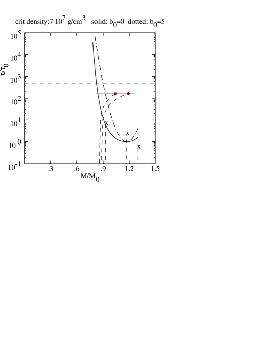
Figure 4: Paths to supernova without accretion (vertical lines) and with accretion (curved lines). The $\tau(M)/\tau_{0}$ curve is approximated by the best fit parabola. The horizontal dashed line corresponds to the age of the universe divided by $\tau_{0}=0.03\,\mathrm{Gyr}$.

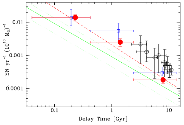
Figure 5: The SNIa rate as a function of delay time from [18]. See text. The key point is that most supernova occur within $0.4\,\mathrm{Gyr}$ of the white dwarf birth but the delay time distribution extends into the multi-Gyr range.

In the case of no accretion (e.g. solitary white dwarfs) the stars age vertically in fig.4. The probability of surviving until reaching the $\tau(M)$ curve is then $1/e$. With the indicated critical density, the two shown high mass DA dwarfs from the Bergeron et al. sample [10] are unlikely to survive to the observed age without accretion but can have a high survival probability if they are accreting and age along the curved paths. Alternatively, the critical density parameter can be increased which results in the parabola moving to the right. Neglecting the fall-off of $F(M(0))$ in the region of $M\approx 1.2$, the greatest supernova rate comes from the minimum of the $\tau(M)$ curve. The two white dwarf masses above and below the minimum have equal intermediate lifetimes leading to a double peak in the ejected mass distribution at these intermediate delay times.

The probability to survive to age $t$ and then make the supernova phase transition in the next interval $dt$ is

$$dP(t)=P_{s}(t)\,dt/\tau(M(t))\quad.$$ (4.20)

The energy released in the phase transition is significantly greater than the energy released afterwards by carbon fusion which results in the star being totally disrupted except for a very small remnant discussed in Section  6. The supernova double distribution as a function of ejected mass, $M(t)$ and delay time $t$ is therefore,

$$\frac{d^{2}N_{SN}}{dM(0)dt}=a_{0}\,F(M(0))\,P_{s}(t)/\tau(M(t))$$ (4.21)

with

$$M(t)=M(0)+c_{0}t\quad.$$ (4.22)

The situation with respect to delay times is well summarized in the graph of ref [18] reproduced here in fig. 5. The recovered delay times [18] with the smallest statistical errors are shown in filled red circles in this graph. Previous measurements [19] with larger statistical errors are shown in open blue squares shifted slightly to the left for clarity. Measurements from 2010 [20] are shown in open black circles. These latter, unfortunately, are in statistical disagreement with the later measurements implying one or more methods are subject to biases or large systematic errors.

	$\mathrm{min}$	$\mathrm{variable}$	$\mathrm{max}$
$\mathrm{scan:}\,$	$5\cdot 10^{7}\,\mathrm{g/cm^{3}}$	$\rho_{c}$	$1.5\cdot 10^{8}\,\mathrm{g/cm^{3}}$
	$0.15\,\mathrm{Gyr}$	$\tau_{0}$	$0.45\,\mathrm{Gyr}$
	0	$b_{0}$	4
	0	$c_{0}$	$0.01\,M_{\odot}/\mathrm{Gyr}$
$\mathrm{require:}\,$	$1.11\cdot 10^{-2}$	$S_{1}$	$1.71\cdot 10^{-2}$
	$0.135$	$R_{21}$	$0.227$
$\mathrm{find:}\,$	$7.3\cdot 10^{7}\,\mathrm{g/cm^{3}}$	$\rho_{c}$	$1.45\cdot 10^{8}\,\mathrm{g/cm^{3}}\;$
	0.18	$\tau_{0}$	0.39
	0.16	$b_{0}$	4
	0	$c_{0}$	$0.01\,M_{\odot}/\mathrm{Gyr}$
	$1.7\cdot 10^{-3}$	$S_{2}$	$3.2\cdot 10^{-3}$
	$1.1\cdot 10^{-4}$	$S_{3}$	$9.3\cdot 10^{-4}$
	0.009	$R_{SN}$	0.023

Table 2: Four parameter monte carlo in phase transition model showing the range of scanned variables, the conditions required, and the resulting minimum and maximum values of the output parameters.

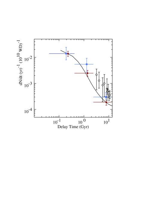
Figure 6: The SNIa rate as a function of delay time in the phase transition model with critical density $\rho_{c}=9\cdot 10^{7}\mathrm{g/cm^{3}},\tau_{0}=0.326\mathrm{Gyr},b_{0}=3.4$, and $c_{0}=0.0016M_{\odot}/\mathrm{Gyr}$. Data is taken from the graph of ref. [18] reprinted here in fig.5 .

In refs. [19] and [18] the supernova rates were divided into three delay time bins bounded by the delay times:

$$t_{1}=0.04Gyr\quad t_{2}=0.4Gyr\quad t_{3}=2.4Gyr\quad t_{4}=13.8Gyr\quad.$$ (4.23)

The average supernova rate in the three bins is

$$S_{i}=\frac{1}{t_{i+1}-t_{i}}\,\int_{t_{i}}^{t_{i+1}}dt\,\frac{dN_{SN}}{dt}\quad.$$ (4.24)

In the phase transition model, the integral over delay times at fixed initial mass can be done analytically so that

$$S_{i}=\frac{1}{t_{i+1}-t_{i}}\,\int dM(0)\int_{t_{i}}^{t_{i+1}}\frac{d^{2}N_{SN}}{dM(0)dt}dt=a_{0}\,\int dM(0)F(M(0))\frac{P_{s}(t_{i})-P_{s}(t_{i+1})}{t_{i+1}-t_{i}}\quad.$$ (4.25)

The total supernova Ia rate is

$$R_{SN}=a_{0}\,\int dM(0)F(M(0))(P_{s}(0)-P_{s}(t_{4}))\quad.$$ (4.26)

4.1 The DD scenario

The approximate linearity of the curve joining the filled red points in fig.5 with a power of approximately $-1$ ($p=-1.12\pm 0.08$) has been interpreted as supporting the DD scenario providing the initial separation distribution of the two white dwarfs is approximately $t^{-1}$. One can question whether this fit requires an implausibly high frequency of binary white dwarfs with a high combined mass. For instance, if we assume in the DD scenario that a collapsing star that would lead to a mass between 1.35 and 1.45 produces with probability $q$ a binary white dwarf system with that total mass, the birthrate (eq.2.4) of such stars and an upper limit to the supernova rate should, from the Salpeter initial mass function, be

$$dN/dt=a_{0}\,q\,\int_{1.35}^{1.45}F(M(0))dM(0)=q\,1.8\cdot 10^{-3}\mathrm{SN/yr/gal}\quad.$$ (4.27)

Since $q$ must be no more than unity this underpredicts the SNIa rate by a factor of about $10$ as is confirmed in more detailed treatments. The alternative path to a binary initial state of white dwarfs namely independent but simultaneous production of white dwarfs from nearby main sequence stars is probably no more likely. In the clean sample of ref.[10] only $13\%$ of white dwarfs are known or suspected to be in double degenerate configurations and, of these, the heaviest dwarf has mass of only $0.66$.

Moreover, with respect to the linear fit, the required inverse $d$ initial separation distribution is not strongly motivated from theory, finiteness requires that the linearity fails at small delay times, and in addition the filled red data points might show a slight negative curvature, i.e. the observed value of $S_{2}$ is some two standard deviations higher than the best fit. As we will see the delay time distribution can be adequately fit in the phase transition model. Returning to the consideration of the phase transition model, from the graph of fig. 5 and the data of ref. [18] we read the $1\sigma$ SNIa rates in the three bins in units of SNIa/yr per prototype galaxy of $10^{10}$ white dwarfs:

$$1.11\cdot 10^{-2}<S_{1}<1.71\cdot 10^{-2}$$

$$1.88\cdot 10^{-3}<S_{2}<3.16\cdot 10^{-3}$$

$$1.44\cdot 10^{-4}<S_{3}<2.33\cdot 10^{-4}$$ (4.28)

or

$$0.135<R_{21}\equiv S_{2}/S_{1}<0.227$$

$$0.008<R_{31}\equiv S_{3}/S_{1}<0.021$$ (4.29)

An advantage of the ratios $R_{21}$ and $R_{31}$ is that they are independent of the $a_{0}$ parameter, i.e. they should be the same for any sample of white dwarfs following the high mass part of the hot white dwarf distribution in fig. 2 regardless of the total number of white dwarfs in the sample. To the extent that the DB dwarfs have the same initial mass function and a similar accretion rate their effect is included in the predicted supernova rates per $10^{10}$ white dwarfs. The phase transition probability would not differ between dwarfs with a thin atmosphere of hydrogen or helium. In the phase transition monte carlo we scan over the four parameters requiring that the resulting $S_{1}$ and $R_{21}$ fall within their $1\sigma$ ranges. The resulting ranges of the other quantities are then tabulated in table 2.

The values for the basic parameters, $\rho_{c}$ and $\tau_{0}$ are not far from the estimates of ref. [9] made prior to the latest data on delay times and ejected mass. Fixing only $S_{1}$ and $R_{21}$ the model predictions span the range of observations for $S_{3}$ and the total supernova rate. In the phase transition model the supernovae fall naturally into two classes, those occuring in isolated dwarfs and those occuring in binary systems with significant accretion onto the white dwarf. The first class contains only those supernovae initiated by the vertical ageing in fig. 4 which would be expected to have a lower $S_{3}$. The second class is represented by the curved paths in fig. 4 and would have higher $S_{3}$ values. If the delay time recovery method is not biased the delay time distribution will be an appropriately weighted average of the two classes. In Table 3 we separate the results in the two classes.

require:	$0.011<S_{1}<0.0171$
	$0.135<R_{21}<0.226$
scan:	$5\cdot 10^{7}\mathrm{g/cm^{3}}<\rho_{c}<1.5\cdot 10^{8}\mathrm{g/cm^{3}}$
	$0.15\mathrm{Gyr}<\tau_{0}<0.45\mathrm{Gyr}$
	$0<b_{0}<4$
	$0<c_{0}<0.002\,M_{\odot}/\mathrm{Gyr}$	$0.002M_{\odot}/\mathrm{Gyr}<c_{0}<0.01\,M_{\odot}/\mathrm{Gyr}$
find:	$0.246\,\mathrm{Gyr}<\tau_{0}<0.389\,\mathrm{Gyr}$	$0.184\,\mathrm{Gyr}<\tau_{0}<0.389\,\mathrm{Gyr}$
	$1.7\cdot 10^{-3}<S_{2}<2.9\cdot 10^{-3}$	$1.7\cdot 10^{-3}<S_{2}<3.2\cdot 10^{-3}$
	$1.1\cdot 10^{-4}<S_{3}<2.6\cdot 10^{-4}$	$1.9\cdot 10^{-4}<S_{3}<9.3\cdot 10^{-4}$
	$0.0068<R_{31}<0.0187$	$0.014<R_{31}<0.091$

Table 3: Four parameter monte carlo in phase transition model separated into the classes with small or large accretion rates. As seen here a larger accretion rate leads to a larger $S_{3}$ as suggested in the data of ref. [20]. Output variables that are insensitive to the accretion rates are not shown.

The parameter space of the phase transition model could be further restricted if the tension between the high delay time measurements could be resolved. If the lower $S_{3}$ values are confirmed, the accretion rates favored by the monte carlo are only about $1\%$ of those allowed by the x-ray data [6] which are themselves only about $1\%$ of the rates that would be required if the full supernova Ia rate were to be explained in the single degenerate scenario. The prediction of low average accretion rates is significant since, with larger accretion rates, the absence of binary partner effects would be puzzling even in the phase transition model.

5 The ejected mass distribution

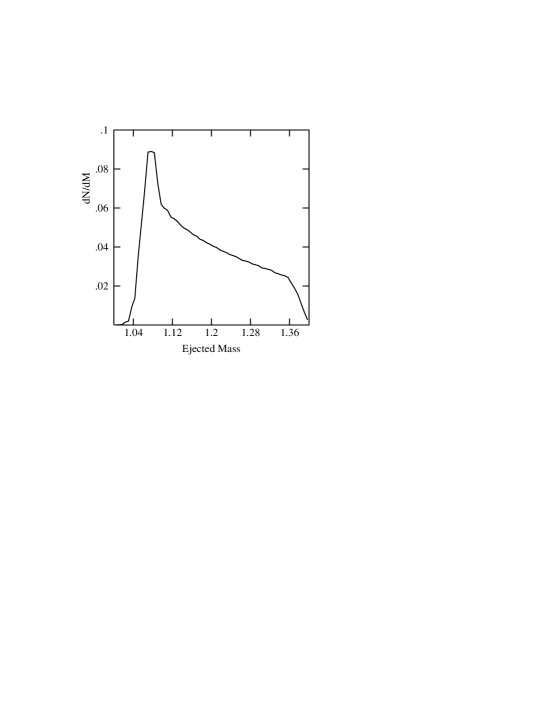
Figure 7: The ejected mass distribution for $\rho_{c}=9\cdot 10^{7}\,\mathrm{g/cm^{3}},\,\tau_{0}=0.326\,\mathrm{Gyr}\,,b_{0}=3.42,\,\mathrm{and}\,c_{0}=0.0016\,M_{\odot}/\mathrm{Gyr}$

Attempts to discover remnants of SNIa have up to now been unsuccessful suggesting the supernova process totally disrupts the white dwarf. This in turn implies in standard scenarios that the ejected mass should be very close to the Chandrasekhar mass. However, recent studies have shown ejected mass distributions extending down to $0.9\,M_{\odot}$ [21]. That would imply remnants extending up to $0.5\,M_{\odot}$. Numerous white dwarfs have been discovered in this mass range but never as supernova remnants. As noted in that reference the ejected mass distribution strongly suggests a sub-Chandrasekhar mechanism such as supplied by the present phase transition model.

From eq. 4.21 we can write the ejected mass distribution between delay times of $t_{i}$ and $t_{i+1}$ assuming the supernova totally disrupts the white dwarf as suggested by the absence of significant remnants and predicted in the present model.

$$\frac{dN}{dM}=a_{0}\int_{t_{i}}^{t_{i+1}}\,dt\,F(M-c_{0}t)\,P_{s}(t)/\tau(M)\quad.$$ (5.30)

Integrating over all delay times, the full ejected mass distribution is

$$\frac{dN}{dM}=a_{0}\int_{0}^{13.8\mathrm{Gyr}}\,dt\,F(M-c_{0}t)\,P_{s}(t)/\tau(M)\quad.$$ (5.31)

Neglecting $c_{0}$, the time integral here can be done analytically. The numerical evaluation of the full ejected mass distribution is shown in fig. 7 for a particular choice of model parameters. The peak of the ejected mass distribution is somewhat lower than indicated in the data of ref. [21] but its narrowness is interesting from the point of view of supernova homogeneity. The peak would move to the right if the critical density parameter were increased.

Figure 8: The ejected mass distribution for the model parameters used in fig. 7 but restricted to the intermediate delay times ($0.4\,\mathrm{Gyr}<t<2.4\,\mathrm{Gyr}$).

As pointed out in section 4, at intermediate delay times the phase transition model predicts a double peak in the ejected mass distribution. This is illustrated in fig. 8.

One should note that the present model for sub-Chandrasekhar supernovae does not preclude a few percent of supernovae coming from accretion to the Chandrsekhar mass as is consistent with the x-ray data [6]. These events arise from white dwarfs punching through the low lifetime region due to rapid accretion. The result would be a second peak in the ejected mass distribution as perhaps observed in the data of ref. [21]. This is independent of the second peak expected in the current model at intermediate delay times as mentioned in section 4.

6 SNIa remnant in the Phase Transition Model

One of the great puzzles in the standard model of SNIa is the absence of detected remnants. In the phase transition model a small bubble of exact susy grows releasing Pauli energy until that energy plus the energy released through fusion is equal at least to the energy required to unbind the shell outside. If one treats the white dwarf as having the average density $3M/(4\pi R^{3})$ the remnant has about $10^{-3}$ of the initial mass [9]. In a more precise treatment of the rapidly decreasing density with radius one might expect this $10^{-3}$ fraction to decrease. This remnant is predominantly made of the scalar partners of the protons, neutrons, and electrons. Since these cannot be supported by degeneracy pressure, the remnant collapses to a black hole of approximately Jupiter mass or smaller. Such a small black hole would be difficult to detect in the supernova aftermath. In the typical galaxy there have been about $10^{8}$ type Ia supernovae since the big bang so the phase transition model would predict this number of low mass black holes in the Milky Way. Charged particles falling into a black hole could be expected to radiate a few percent of their rest mass. This prediction could perhaps be tested in cosmic x-ray backgrounds [22] ,[23] ,[24]. In addition many stars could have captured one of these small black holes which might then be manifested by massive objects orbiting at large angle from the solar disks similar to the apparent “planet nine” in our own solar system. Such black hole planets might also be expected to have their own moons and/or accretion disks. The complete treatment of the growth of a susy bubble in a dense star and its remnant is a complicated dynamical calculation which has only been preliminarily considered in refs. [14],[15],[16].

7 Summary

The phase transition model has a number of advantages relative to the standard model explosion at the Chandrasekhar mass. The delay time distribution although not linear in a log-log plot can easily fit the data. The ejected mass distribution naturally peaks below the Chandrasekhar mass. The total supernova rate is related to known single white dwarf mass distributions unlike the situation in the standard model which depends on unknown binary distributions and which, with plausible assumptions, greatly underestimates the total rate. The absence of observed remnants which is puzzling in the standard model is easily understood in the phase transition model which also makes an interesting prediction of remnant effects. The sphericity of supernova events and the absence of shadowing by a binary partner are predicted in the phase transition model with low accretion rates but remain puzzling in the standard model. In the DD scenario one must wonder why there are no observations of binary white dwarf systems with near Chandrasekhar combined mass and how the homogeneity of normal SNIa which is crucial to dark energy measurements is maintained. In the DD scenario one would expect that the peak of the white dwarf distribution at $0.6$ would lead to a secondary peak at $1.2$ due to a coalescence of binary white dwarfs. Indeed in fig. 2 there seems to be such a secondary peak but it is known [11] that this is purely an artifact of the treatment of the high mass tail.

Significant discussions with Peter Biermann, Ken Olum, and Akos Bogdan contributing to the work of this paper are gratefully acknowledged.

References

-
[1]
Chandrasekhar, S., Astrophys. J. 74, 81 (1931)
Chandrasekhar, S., Introduction to the Study of Stellar Structure, Dover Publications, New York (1939). - [2] Whelan, J. and Iben, I.J., Astrophys. J. , 186, 1007 (1973).
- [3] Webbink, R.F., Astrophys. J. 277, 355 (1984).
- [4] Hillebrandt, W., & Niemeyer, J. C., Ann. Rev. Astron. & Astrophys. 38, 191 (2000), (astro-ph/0006305).
- [5] Maoz, D. and Mannucci, Filippo, (ArXiv:1111.4492v2).
- [6] Gilfanov, M., & Bogdán, Á., Nature 463, 924 (2010).
- [7] DiStefano, R., Astrophys. J. 712, 728 (2010).
- [8] Bulla, M. et al. Month. Not. Roy. Astr. Soc. (2016), (ArXiv:1510.04128v1).
- [9] Biermann, P. and Clavelli, L., Phys. Rev. D 84,023001 (2011) (ArXiv:1011.1687v2).
- [10] Bergeron, P.,Leggett S.K., and Ruiz, Maria, Astro-ph/0011286.
- [11] Madej, J., Nalezyty, M., and Althaus, L.G., Astron. & Astroph. 419, L5 (2004).
- [12] Ciechanowska, A., Nalezyty, M., Majczyna, A., Madej, J., 15th European Workshop on White Dwarfs, ASP Conference Series, Vol 372 (2007).
- [13] Clavelli, L. and Karatheodoris, G.,hep-ph/0403227 Phys. Rev. D72, 035001 (2005).
- [14] Clavelli, L. and Perevalova, I., hep-ph/0409194, Phys. Rev. D71, 055001 (2005).
- [15] Clavelli, L., hep-ph/0506215, Phys. Rev. D72, 055005 (2005), erratum Phys. Rev. D73, 039901 (2006).
- [16] Clavelli, L., hep-ph/0602024, High Energy Density Physics, Vol 2, Nos 3-4, 97-103 (2006).
- [17] Coleman, S., Phys. Rev. D15, 2929 (1977); Callan, C.G. & Coleman, S., Phys. Rev. D16, 1762 (1977); Coleman, S., and DeLuccia, F., Phys. Rev. D21, 3305 (1980).
- [18] Maoz, D., Mannucci, F., and Brandt, T., ArXiv:1206.0465.
- [19] Maoz, D.,Mannucci, F., Li, W., Filipenko, A.V., Della Valle, M., and Panagia, N., Month. Not. Roy. Astr. Soc. , 412, 1508 (2011).
-
[20]
Maoz, D., Sharon, K., and Gai-Yam, A., Astrophys. J. , 722, 1879 (2010)
Maoz, D. and Badenes, C., Month. Not. Roy. Astr. Soc. , 407, 1314 (2010). - [21] Scalzo, R.A., Ruiter, A.J., and Sim, S.A., Month. Not. Roy. Astr. Soc. , 445, 2535 (2014), ArXiv:1402.6842.
- [22] Shakura, N.I. and Sunyaev, R.A., Astron. & Astroph. 24, 337 (1973).
- [23] Moran, Edward C. et al., Astrophys. J. 556, L75 (2001), Astro-ph/0106519 .
- [24] Moretti, A. et al., Astron. & Astroph. 548, A87 (2012), ArXiv:1210.6377.