Electronic structure and magnetism of samarium and neodymium adatoms on free-standing graphene

Abstract

The electronic structure of selected rare-earth atoms adsorbed on a free-standing graphene was investigated using methods beyond the conventional density functional theory (DFT+U, DFT+HIA and DFT+ED). The influence of the electron correlations and the spin-orbit coupling on the magnetic properties has been examined. The DFT+U method predicts both atoms to carry local magnetic moments (spin and orbital) contrary to a nonmagnetic $f^{6}$ ($J=0$) ground-state configuration of Sm in the gas phase. Application of DFT${}+{}$Hubbard-I (HIA) and DFT${}+{}$exact diagonalization (ED) methods cures this problem, and yields a nonmagnetic ground state with six $f$ electrons and $J=0$ for the Sm adatom. Our calculations show that Nd adatom remains magnetic, with four localized $f$ electrons and $J=4.0$. These conclusions could be verified by STM and XAS experiments.

I Introduction

Adsorption of atoms and molecules provides a way to control and modify the electronic properties of graphene Katsnelson (2012). Adsorption of alkali and transition metals on graphene was investigated extensively in recent years.Eelbo et al. (2013); Sessi et al. (2014); Wehling et al. (2011); Virgus et al. (2014) There are much less studies of interaction between rare-earth atoms and graphene. Since the bonding character of the $sp$ elements and transition metals is different from that of strongly localized $4f$ metals, a different behavior of the rare-earth atoms adsorbed on graphene is expected. In the pioneering work Liu et al. (2010), the first-principles theory has been applied to several rare-earth adatoms on graphene, together with the scanning tunneling microscopy (STM) experiments. It was shown that the hollow site of graphene is the energetically favorable adsorption site for all the rare-earth adatoms. Magnetic moments have been reported for all adatoms studied.

Accurate description of the electronic and magnetic properties of the $f$-electron systems remains a challenge in condensed matter physics. The standard density-functional theory (DFT) proves to be inadequate due to the self-interaction error Cohen et al. (2008). For this reason, theories like self-interaction correction Perdew and Zunger (1981), hybrid functionals Becke (1993) or treatment of the 4$f$-shell as core-like Skriver (1985) have been explored. In Ref. Liu et al., 2010, the $f$-states of the rare-earth adatoms were treated as a part of the atomic core and were fixed in a given configuration. That places some limits on the validity of acquired conclusions about the magnetic character of the $f$-manifold.

In this paper, we re-examine the electronic and magnetic structure of two rare-earth adatoms (Sm and Nd) on graphene making use of the rotationally invariant formulation of the DFT+U method Liechtenstein et al. (1995). In order to incorporate the dynamical electron correlations, we employ the exact diagonalization (ED) method to solve a multi-orbital single-impurity Anderson model Hewson (1993) whose parameters are extracted from DFT calculations. This method is conceptually similar to earlier calculations of bulk rare-earth materials.Thunström et al. (2009); Locht et al. (2016)

In Sec. II we describe the DFT+U and DFT+ED methods which we use to calculate the electronic structure and magnetic properties of the adatoms on graphene. Special attention is paid to modifications of the DFT+U due to the spin-orbit coupling (SOC). In Sec. III we describe the results of the DFT+U, DFT+Hubbard I (HIA) and DFT+ED calculations of Sm adatom on graphene (Sm@GR). It is shown that the $f^{6}$ shell of Sm with the nonmagnetic singlet ground state cannot be described correctly by DFT+U. The use of DFT+HIA and DFT+ED solves this problem. In Sec. IV we address the electronic and magnetic character of a rare-earth adatom with the local moment, taking as an example Nd adatom on graphene (Nd@GR). A comparison between DFT+U and DFT+HIA is given. Reasonable agreement between the DFT+U and DFT+HIA $f$-projected density of states (DOS) is demonstrated.

II Computational methods

The conventional band theory fails to correctly describe the strongly localized 4$f$ states due to the oversimplified treatment of electron correlations, as it is often seen in the applications of DFT to $f$-electron materials. Here, we use the correlated band theory (DFT+U) method, which consists of DFT augmented by a correcting energy of a multiband Hubbard type.

In order to describe the structural, electronic and magnetic properties of the rare-earth adatoms on graphene, we use the supercell shown in Fig. 1. This $4\times 4\times 1$ supercell includes 32 carbon atoms, and the rare-earth adatom is placed in the hexagonal hollow position. First, the structure relaxation was performed employing the standard Vienna ab initio simulation package (VASP) Kresse and Furthmuller (1996) together with the projector augmented-wave method (PAW) Blochl (1994) without SOC. We used the DFT+U method with the exchange-correlation functional of Perdew, Burke and Ernzerhof (PBE).Perdew et al. (1996) The Coulomb $U$ values of 6.76 eV (Nd) and 6.87 eV (Sm), and the exchange $J$ of 0.76 eV were used, which are in the commonly accepted range of $U$ and $J$ for the rare earthsvan der Marel and Sawatzky (1988). The optimal heights for the rare-earth adatoms above the graphene sheet are found as $h_{\rm Sm}=4.58$ bohr and $h_{\rm Nd}=4.55$ bohr.

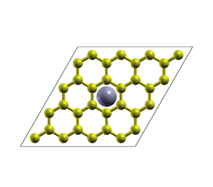
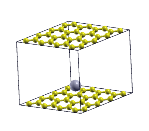
Figure 1: Schematic supercell model for rare-earth impurity on graphene.

The structural information obtained from the VASP simulations was used as an input for further electronic-structure calculations that employ the relativistic version of the full-potential linearized augmented plane-wave method (FLAPW) Wimmer et al. (1981), in which the SOC is included in a self-consistent second-variational procedure Shick et al. (1997). This two-step approach synergetically combines the speed and efficiency of the highly optimized VASP package with the state-of-the-art accuracy of the FLAPW method.

II.1 DFT+U with spin-orbit coupling

When the spin-orbit coupling is taken into account, the spin is no longer a good quantum number, and the electron-electron interaction energy $E^{\rm ee}$ in the DFT+U rotationally-invariant total-energy functional Liechtenstein et al. (1995) has to be modified Solovyev et al. (1998) to

$$E^{\rm ee}=\frac{1}{2}\sum_{\gamma_{1}\gamma_{2}\gamma_{3}\gamma_{4}}n_{\gamma_{1}\gamma_{2}}\Big{(}V^{\rm ee}_{\gamma_{1}\gamma_{3};\gamma_{2}\gamma_{4}}-V^{\rm ee}_{\gamma_{1}\gamma_{3};\gamma_{4}\gamma_{2}}\Big{)}n_{\gamma_{3}\gamma_{4}}\;,$$ (1)

where $V^{\rm ee}$ is an effective on-site Coulomb interaction expressed in terms of Slater integrals that are linked to the intra-atomic repulsion $U$ and exchange $J$, see Eq. (3) in Ref. Shick et al., 1999. The essential feature of the generalized total energy functional (1) is that it contains spin-off-diagonal elements of the on-site occupation matrix $n_{\gamma_{1}\gamma_{2}}\equiv n_{m_{1}\sigma_{1},m_{2}\sigma_{2}}$ which become important in the presence of large SOC.

For a given set of spin-orbitals $\{\phi_{m\sigma}\}$, we minimize the DFT+U total energy functional. It gives the Kohn–Sham equations for a two-component spinor $\bm{\Phi}_{i}=\left(\begin{array}[]{c}\Phi^{\uparrow}_{i}\\ \Phi^{\downarrow}_{i}\end{array}\right)$,

$$\sum_{\beta}\Bigl{[}-\nabla^{2}+\hat{V}_{\rm eff}+\xi\,(\bm{l}\cdot\bm{s})\Bigr{]}_{\alpha,\beta}\Phi^{\beta}_{i}(\bm{r})=e_{i}\Phi^{\alpha}_{i}(\bm{r})\;,$$ (2)

where the effective potential $\hat{V}_{\rm eff}$ is a sum of the standard (spin-diagonal) DFT potential and the on-site electron-electron interaction potential $V_{U}$,

$$\hat{V}^{\alpha,\beta}_{U}=\sum_{m,m^{\prime}}|\phi_{\alpha m}\rangle\Bigl{(}W^{\alpha m,\beta m^{\prime}}-\delta_{m,m^{\prime}}\delta_{\beta,\alpha}W_{\rm dc}^{\alpha}\Bigr{)}\langle\phi_{\beta m^{\prime}}|\,,$$ (3)

where

$$W^{\alpha m,\beta m^{\prime}}=\sum_{p\sigma,q\sigma^{\prime}}\Big{(}\langle m^{\prime}\beta,p\sigma|V^{ee}|m\alpha,q\sigma^{\prime}\rangle\Big{.}$$

$$\Big{.}-\langle m^{\prime}\beta,p\sigma|V^{ee}|q\sigma^{\prime},m\alpha\rangle\Big{)}n_{p\sigma,q\sigma^{\prime}}$$ (4)

and $W_{\rm dc}^{\alpha}$ is the double-counting correction. The most commonly used form of $W^{\sigma}_{\rm dc}$ is the so-called “fully localized” (or atomic-like) limit (FLL) Liechtenstein et al. (1995), $W^{\sigma}_{\rm dc}=U(n_{f}-1/2)-J(n^{\sigma}_{f}-1/2)$. Another form of the DFT+U functional is often called as “around-mean-field” (AMF) limit of the DFT+U Anisimov et al. (1991), $W^{\sigma}_{\rm dc}=Un^{-\sigma}_{f}+\frac{2l}{(2l+1)}(U-J)n^{\sigma}_{f}$. The operator $|\phi_{\alpha m}\rangle\langle\phi_{\beta m^{\prime}}|$ in Eq. (3) acts on the two-component spinor wave function $\bm{\Phi}$ as $|\phi_{\alpha m}\rangle\langle\phi_{\beta m^{\prime}}|\Phi^{\beta}\rangle$.

In addition to the spin-dependent DFT potential, the DFT+U method creates a spin- and orbitally-dependent on-site “$+U$” potential, which enhances orbital polarization beyond the polarization given by the DFT alone (where it comes from the SOC only). We also note that the DFT contributions to the effective potential $\hat{V}_{\rm eff}$ in Eq. (2) are corrected to exclude the double-counting of the $f$-states nonspherical contributions to the DFT and DFT+U parts of the potential. The nonspherical part of the DFT potential is expanded in terms of the lattice harmonics $K_{\nu}$, $V^{\rm NSH}_{\rm DFT}(\bm{r})=\sum_{\nu}V_{\nu}(r)K_{\nu}(\hat{\bm{r}})$. The DFT contributions to the muffin-tin nonspherical matrix elements, that are proportional to $\langle lm_{1}|K_{\mu}|lm_{2}\rangle$ for $l=3$ orbital quantum number, are removed.

II.2 DFT combined with the Anderson impurity model (DFT+ED)

To proceed beyond DFT+U in the electronic structure of the 4$f$ adatoms on graphene, we make use of the “DFT++” methodology Lichtenstein and Katsnelson (1998). We consider the one-particle Hamiltonian found from ab initio electronic structure calculations plus the on-site Coulomb interaction describing the $f$-electron correlation of an adatom. The effects of the Coulomb interaction on the electronic structure are described by a one-particle selfenergy $\Sigma(z)$ (where $z$ is a (complex) energy), which is calculated in a multiorbital Anderson impurity model,

$$H_{\rm imp}=\sum_{\begin{subarray}{c}kmm^{\prime}\\ \sigma\sigma^{\prime}\end{subarray}}[\epsilon^{k}]_{mm^{\prime}}^{\sigma\;\;\sigma^{\prime}}b^{\dagger}_{km\sigma}b_{km^{\prime}\sigma^{\prime}}+\sum_{m\sigma}\epsilon_{f}f^{\dagger}_{m\sigma}f_{m\sigma}$$

$$+\sum_{mm^{\prime}\sigma\sigma^{\prime}}\bigl{[}\xi\,(\bm{l}\cdot\bm{s})+\Delta_{\rm CF}\bigr{]}_{mm^{\prime}}^{\sigma\;\;\sigma^{\prime}}f_{m\sigma}^{\dagger}f_{m^{\prime}\sigma^{\prime}}$$

$$+\sum_{\begin{subarray}{c}kmm^{\prime}\\ \sigma\sigma^{\prime}\end{subarray}}\Bigl{(}[V^{k}]_{mm^{\prime}}^{\sigma\;\;\sigma^{\prime}}f^{\dagger}_{m\sigma}b_{km^{\prime}\sigma^{\prime}}+{h.c.}\Bigr{)}$$

$$+\frac{1}{2}\sum_{\begin{subarray}{c}mm^{\prime}m^{\prime\prime}\\ m^{\prime\prime\prime}\sigma\sigma^{\prime}\end{subarray}}U_{mm^{\prime}m^{\prime\prime}m^{\prime\prime\prime}}f^{\dagger}_{m\sigma}f^{\dagger}_{m^{\prime}\sigma^{\prime}}f_{m^{\prime\prime\prime}\sigma^{\prime}}f_{m^{\prime\prime}\sigma}.$$ (5)

Here $f^{\dagger}_{m\sigma}$ creates an electron in the 4$f$ shell and $b^{\dagger}_{m\sigma}$ creates an electron in the “bath” that consists of those host-band states that hybridize with the impurity 4$f$ shell. The energy position $\epsilon_{f}$ of the impurity level, and the bath energies $\epsilon^{k}$ are measured from the chemical potential $\mu$. The parameters $\xi$ and $\Delta_{\rm CF}$ specify the strength of the SOC and the size of the crystal field at the impurity. The parameter matrices $V^{k}$ describe the hybridization between the $f$ states and the bath orbitals at energy $\epsilon^{k}$.

The band Lanczos method Kolorenc et al. (2012), paired with an efficient truncation of the many-body Hilbert space Kolorenč et al. (2015) is employed to find the lowest-lying eigenstates of the many-body Hamiltonian $H_{\rm imp}$ for a given number $n_{f}$ of correlated electrons, and to calculate the one-particle Green’s function $[G_{\rm imp}(z)]_{mm^{\prime}}^{\sigma\;\;\sigma^{\prime}}$ in the subspace of the $f$ orbitals. The selfenergy $[\Sigma(z)]_{mm^{\prime}}^{\sigma\;\;\sigma^{\prime}}$ is then obtained from the inverse of the Green’s function matrix $G_{\rm imp}$.

Once the selfenergy is known, the local Green’s function $G(z)$ for the electrons in the $f$ manifold of the rare-earth adatom is calculated as

$$G(z)=\Big{[}{G}_{0}^{-1}(z)+\Delta\epsilon-\Sigma(z)\Big{]}^{-1}\,,$$ (6)

where ${G}_{0}(z)$ is the noninteracting Green’s function, and $\Delta\epsilon$ is chosen to ensure that $n_{f}=\pi^{-1}\mathop{\rm Im}\mathop{\rm Tr}\int_{-\infty}^{E_{{\rm F}}}{\rm d}E\,G(E-{\rm i}0)$ is equal to the given number of correlated electrons. Subsequently, we evaluate the occupation matrix in the 4$f$ shell, $n_{\gamma_{1}\gamma_{2}}=\pi^{-1}\mathop{\rm Im}\int_{-\infty}^{E_{\rm{F}}}{\rm d}E\,[G(E-\rm i0)]_{\gamma_{1}\gamma_{2}}$. This matrix is used to construct an effective DFT+U potential ${V}_{U}$, Eq. (3), which is inserted into Kohn–Sham Eqs. (2). The DFT+U Green’s function $G_{U}(z)$ is evaluated from the eigenvalues and eigenfunctions of Eq. (2), represented in the FLAPW basis, and then it is used to calculate an updated noninteracting Green’s function ${G}_{0}^{-1}(z)=G_{U}^{-1}(z)+V_{U}(z)$. In each iteration, a new value of the 4$f$-shell occupation is obtained. Subsequently, a new self-energy $\Sigma(z)$ corresponding to the updated $f$-shell occupation is constructed. Finally, the next iteration is started by evaluating the new local Green’s function, Eq. (6). The steps are iterated until self-consistency over the charge density is reached.

When the hybridization between the $f$ states and the bath orbitals is weak, one can neglect the first and fourth terms in Eq. (II.2), and the Anderson impurity model is reduced to the atomic model. This approximation is called Hubbard-I approximation (HIA). The use of HIA allows us to substantially reduce the computational cost needed for the exact diagonalization of the Hamiltonian (II.2). The same procedure for the charge-density self-consistency is used for DFT+HIA. Further details of the DFT+HIA implementation in the FP-LAPW basis are described in Ref. Shick et al., 2009.

III Samarium on graphene

III.1 DFT+U

We start with the application of the DFT+U approach to Sm@GR. The Slater integrals that define the on-site Coulomb interaction are chosen as $F_{0}=6.87$ eV, $F_{2}=9.06$ eV, $F_{4}=6.05$ eV, and $F_{6}=4.48$ eV. They correspond to Coulomb $U=6.87$ eV and Hund exchange $J=0.76$ eV. The spin ($M_{S}$) and orbital ($M_{L}$) magnetic moments are given in Table 1 together with the occupation of the Sm $4f$ orbitals $n_{f}$. In these calculations, the magnetization (spin${}+{}$orbital) is constrained along the crystallographic axes: $x,y$ (in plane), and $z$ (out of plane). The DFT+U-FLL yields a solution with both $M_{S}$ and $M_{L}$ non-zero, and $n_{f}$ very close to six. Thus the FLL flavor of the DFT+U gives an $f^{6}$ magnetic ground state with the total moment $M_{J}$ = 2.9 $\mu_{B}$. On the contrary, the DFT+U-AMF converges to a practically nonmagnetic $f^{6}$ ground state with all $M_{S}$, $M_{L}$ and $M_{J}$ close to zero (Table 1).

Table 1: Spin ($M_{S}$), and orbital ($M_{L}$) magnetic moments (in $\mu_{B}$) and $4f$ occupation $n_{f}$ of the Sm adatom on graphene for three different directions of the magnetization $M$: $x,y$ (in plane), and $z$ (out of plane).

Sm@GR	FLL			AMF
	$n_{f}$	$M_{S}$	$M_{L}$	$n_{f}$	$M_{S}$	$M_{L}$
$M||x$	5.94	5.85	$-2.90$	5.94	0.09	$-0.04$
$M||y$	5.94	5.86	$-2.91$	5.94	0.09	$-0.03$
$M||z$	5.94	5.84	$-2.93$	5.94	0.19	$-0.10$

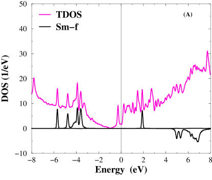
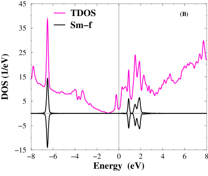
Figure 2: The total (TDOS) and spin-resolved $f$-orbital density of states for the Sm adatom on graphene calculated with DFT+U-FLL (A) and DFT+U-AMF (B).

The calculated total density of states (TDOS, for both spins, and per unit cell) and the $f$-orbital spin-resolved DOS for Sm adatom calculated with DFT+U-FLL and DFT+U-AMF are shown in Fig. 2. The DFT+U-FLL yields a mean-field solution with broken symmetry. This is because the part of the Coulomb interaction treated in the Hartree–Fock-like approximation is transformed into the exchange splitting field. This exchange field is several eV strong (see Fig. 2) and by far exceeds any imaginable external magnetic field. This exchange field is reduced to almost zero in the DFT+U-AMF calculations. The DFT+U is not based on any kind of atomic coupling scheme ($LS$ or $jj$), since it determines a set of single-particle orbitals that variationally minimize the total energy. The AMF calculated $f^{6}$ nonmagnetic ground state corresponds to the Slater determinant formed of six equally populated $j=5/2$ orbitals.

III.2 DFT+HIA

The observation that two different flavors of DFT+U yield different results for the magnetic properties is similar to $fcc$-Am where the DFT+U results strongly depend on the choice of the DFT+U double counting Shick et al. (2006). This situation is quite alarming, and indicates that one has to go beyond the static mean-field approximation to accurately model these systems. Such an improved approximation was introduced in Sec. II.2 where the Coulomb potential $V_{U}$, Eq. (3), is calculated from the occupation matrix $n_{m_{1}\sigma_{1},m_{2}\sigma_{2}}$ corresponding to a multi-reference many-body wave function instead of a single Kohn–Sham determinant. The many-body wave function is the ground state of the impurity model from Eq. (II.2) with the following parameters: the Slater integrals are the same as those used in the DFT+U calculations, the spin-orbit parameter $\xi=0.16$ eV was determined from DFT calculations, and the crystal-field effects are neglected, $\Delta_{\rm CF}=0$.

First, we excluded the hybridization between the $f$ states and the bath orbitals in Eq. (II.2), and used DFT+HIA. The occupation of the 4$f$ shell self-consistently determined from Eq. (2) is $\langle n_{f}\rangle=5.95$ (FLL double counting) and $\langle n_{f}\rangle=5.98$ (AMF double counting). When we alternatively fix $\epsilon_{f}$ in Eq. (II.2) to $-W_{\rm dc}$ from Eq. (3), we obtain the occupation $\langle n_{f}\rangle=6.0$. It means that all $f$-electrons of Sm are fully localized. The ground state of the 4$f$ shell is a nonmagnetic singlet with all angular moments equal to zero ($S=L=J=0$). The $f$-orbital DOS obtained from Eq. (6) is shown in Fig. 3 (A). There is practically no difference between the different double-counting variants, FLL or AMF, in Eq. (2).

III.3 DFT+ED

Next, we determine the bath parameters $V^{k}$ and $\epsilon^{k}$, assuming that the DFT represents the noninteracting model. That is, we associate the DFT Green’s function ${G}_{\rm{DFT}}(z)$ with the Hamiltonian (II.2) when the coefficients of the Coulomb interaction matrix are set to zero ($U_{mm^{\prime}m^{\prime\prime}m^{\prime\prime\prime}}=0$). The hybridization function ${\Delta(\epsilon)}$ is then estimated as ${\Delta}(\epsilon)=\mathop{\rm Im}\mathop{\rm Tr}[G^{-1}_{\rm DFT}(\epsilon-{i0})]$.

A detailed inspection shows that the hybridization matrix is, to a good approximation, diagonal in the $\{j,j_{z}\}$ representation. Thus, we assume the first and fourth terms in Eq. (II.2) to be diagonal in $\{j,j_{z}\}$. Hence we only need to specify one bath state (six orbitals) with $\epsilon^{k=1}_{j=5/2}$ and $V^{k=1}_{j=5/2}$, and another bath state (eight orbitals) with $\epsilon^{k=1}_{j=7/2}$ and $V^{k=1}_{j=7/2}$. Assuming that the most important hybridization occurs in the vicinity of the Fermi level $E_{\rm F}$, the numerical values of the hybridization parameters $V^{k=1}_{5/2,7/2}$ are found from the relation Gunnarsson et al. (1989) $\pi\sum_{k}{|V_{j}^{k}|}^{2}\delta(\epsilon_{j}^{k}-\epsilon)=-\Delta(\epsilon)/N_{j}$ averaged over the energy interval, $E_{\rm F}-0.5$ eV $\leq\epsilon\leq E_{\rm F}+0.5$ eV, with $N_{j}=6$ for $j=5/2$ and $N_{j}=8$ for $j=7/2$. The bath-state energies $\epsilon^{k=1}_{5/2,7/2}$ shown in Table 2 are then adjusted to approximately reproduce the DFT occupations of the $f$ states, $n_{f}^{5/2}$ and $n_{f}^{7/2}$. Note that the magnitudes of the hybridization parameters $V$ are very small indicating the localized nature of the 4$f$-states.

Table 2: $f$-states occupations $n_{f}^{5/2}$ and $n_{f}^{7/2}$, and bath-state parameters $\epsilon^{1}_{5/2}$, $\epsilon^{1}_{7/2}$, $V^{1}_{5/2}$, $V^{1}_{7/2}$ (all energies in eV) for Sm and Nd adatoms determined from DFT calculations.

Adatom	$n_{f}^{5/2}$	$n_{f}^{7/2}$	$\epsilon^{1}_{5/2}$	$V^{1}_{5/2}$	$\epsilon^{1}_{7/2}$	$V^{1}_{7/2}$
Sm	5.72	0.36	0.025	0.071	$-0.500$	0.077
Nd	3.49	0.14	0.050	0.085	$-0.500$	0.087

The occupation of the 4$f$ shell self-consistently determined from Eq. (2) is $\langle n_{f}\rangle=5.95$ (FLL double counting) and $\langle n_{f}\rangle=5.97$ (AMF double counting). Since the occupation is very close to $\langle n_{f}\rangle=6.0$, we kept $\epsilon_{f}$ in Eq. (II.2) at $\langle n_{f}\rangle=6.0$. The ground state of the cluster formed by the 4$f$ shell and the bath is a nonmagnetic singlet with all angular moments equal to zero ($S=L=J=0$). In this ground state, there are $\langle n_{f}\rangle=6.0$ electrons in the $4f$ shell and $\langle n_{\rm bath}\rangle=8.0$ electrons in the bath states. The ground-state expectation values of the angular moments of the $4f$ shell are calculated as $S_{f}=2.92$, $L_{f}=2.92$, and $J_{f}=0.03$. The singlet ground state is separated from the first excited state (triplet) by a gap of 50 meV. The $f$-orbital density of states obtained from Eq. (6) is shown in Fig. 3 (B). Comparison with DFT+HIA, Fig. 3 (A), demonstrates similar features with about 1 eV upward energy shift. Also, we have examined the double-counting choice in Eq. (2), and found practically no difference between the different double-counting variants, FLL or AMF.

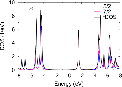
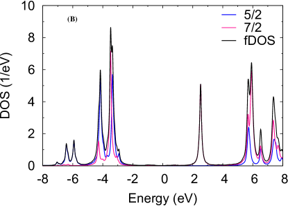
Figure 3: $f$-electron density of states (fDOS, and $j=5/2$, $7/2$ projected) for the Sm atom in Sm@GR resulting from DFT+HIA calculations (A); fDOS, and $j=5/2$, $7/2$ projected fDOS, for the Sm atom in Sm@GR from DFT+ED (B).

III.4 Implications for x-ray absorption spectroscopy

Information about the $4f$ states can be gleaned from the x-ray absorption spectroscopy (XAS). In these experiments, the intensities $I_{5/2}$ ($3d_{5/2}\rightarrow 4f_{5/2,7/2}$) and $I_{3/2}$ ($3d_{3/2}\rightarrow 4f_{5/2}$) of the individual absorption lines are measured and the branching ratio $B=I_{5/2}/(I_{3/2}+I_{5/2})$ is evaluated Moore and van der Laan (2009). We compute the branching ratio $B$ for core to valence $3d$–$4f$ transition by obtaining $n_{5/2}$ and $n_{7/2}$ from the local occupation matrix $n_{\gamma_{1}\gamma_{2}}$ and making use of the sum rule Moore and van der Laan (2009),

$$B=\frac{3}{5}\;-\;\frac{2}{5}\,\frac{n_{f}^{7/2}-\frac{4}{3}\,n_{f}^{5/2}}{14-n_{f}}\,.$$ (7)

Table 3: Occupation $n_{f}$, values of $n_{f}^{5/2}$ and $n_{f}^{7/2}$, and branching ratio $B$ for Sm@GR. The atomic theory values Moore and van der Laan (2009) for $n_{f}=6$ in the $LS$ and $jj$ coupling schemes are also given.

Sm@GR	$n_{f}$	$n_{f}^{5/2}$	$n_{f}^{7/2}$	$B$
DFT+U-FLL	5.94	3.33	2.60	0.69
DFT+U-AMF	5.94	5.87	0.07	0.985
DFT+HIA-FLL	5.95	3.80	2.14	0.745
DFT+ED-FLL	5.95	3.81	2.14	0.75
DFT+HIA-AMF	5.98	3.82	2.16	0.75
DFT+ED-AMF	5.97	3.82	2.16	0.75
atomic $LS$	6	3.14	2.86	0.67
atomic $jj$	6	6.00	0.00	1.00

The DFT+U-FLL as well as DFT+HIA and DFT+ED yield the branching ratios close to the atomic $LS$-coupling limit (Table 3). On the contrary, the DFT+U-AMF value is close to the $jj$-coupling atomic value $B=1.0$. It is rather well established that the rare-earth atoms with the localized $f$ shell are well described by the $LS$-coupling scheme, and our DFT+HIA and DFT+ED calculations, which are not bound by any particular atomic coupling scheme, illustrate once again the validity of the conventional atomic theory. At the same time, the DFT+U-AMF does not have the proper atomic limit since it is very far from the $LS$-coupling scheme.

As we have shown, the use of DFT+U for Sm on graphene can lead to erroneous conclusions about the magnetic character of the Sm adatom. In fact, recent DFT+U calculations Li et al. (2016) for the rare-earth atoms embedded in graphene, including Sm, report it to carry large spin and orbital magnetic moments. We think that the magnetic character of Sm atom in graphene was not determined correctly Li et al. (2016).

IV Neodymium on graphene

IV.1 DFT+HIA

Theoretical evaluation of the local magnetic moments of the rare-earth atoms adsorbed on a nonmagnetic substrate is an important issue in the context of creating a single 4$f$-atom magnet Miyamachi et al. (2013); Donati et al. (2014). As an example of the rare-earth adatom, where the local moment is expected to exist from the atomic $LS$-coupling scheme arguments, we consider the case of Nd@GR. For the DFT+HIA calculations, the Slater integrals $F_{0}=6.76$ eV, $F_{2}=9.06$ eV, $F_{4}=6.05$ eV, and $F_{6}=4.48$ eV were chosen. They corresponds to Coulomb $U=6.76$ eV and exchange $J=0.76$ eV. The spin-orbit parameter was determined by DFT that yields $\xi=0.13$ eV. The bath parameters were evaluated using the same procedure as for Sm@GR, they are listed in Table 2. It is seen that the hybridization strength in Nd@GR is rather similar to Sm@GR. This weak hybridization allows us to use the simpler DFT+HIA method.

The ground state of the Nd atom on graphene, the solution of Eq. (2), has $\langle n_{f}\rangle=3.66$ $f$ electrons. Note that Nd atom in solid-state compounds commonly has a valency $3+$, and the deviation from the atomic-like $f^{4}$ configuration is thus not surprising. The ground state has degeneracy of nine, and the expectation values of the $4f$-shell moments are $S_{f}=1.96$, $L_{f}=5.95$, and $J_{f}=4.00$. These values are consistent with the ${}^{5}I_{4}$ $LS$-coupled $f^{4}$ atomic ground state. The degenerate character of the ground state dictates the presence of local moment for Nd@GR. The XAS branching ratio $B=0.715$ is calculated, and can be verified experimentally.

Table 4: Spin ($M_{S}$), and orbital ($M_{L}$) magnetic moments (in $\mu_{B}$) and $4f$ occupation $n_{f}$ of Nd@GR for three different directions of the magnetization $M$: $x,y$ (in plane) and $z$ (out of plane).

Nd@GR	$n_{f}$	$M_{S}$	$M_{L}$
$M||x$	3.78	3.70	$-4.59$
$M||y$	3.78	3.71	$-4.60$
$M||z$	3.78	3.69	$-2.58$

IV.2 DFT+U

Since we have shown that DFT+U+AMF does not have the correct atomic limit (it is not close to the $LS$-coupling scheme), we apply only the DFT+U-FLL approach to Nd@GR. It yields non-zero spin $M_{S}$ and orbital $M_{L}$ magnetic moments, which are given in Table 4 together with the occupation of the Nd adatom $f$ orbitals, $n_{f}$. In these calculations, the magnetization (spin${}+{}$orbital) is constrained along the crystallographic axes: $x,y$ (in plane) and $z$ (out of plane). Note that $M_{S}$ and $M_{L}$ have different physical meaning than $S_{f}$ and $L_{f}$ in DFT+ED calculations: they represent the projections of the spin and orbital moments on the selected axis, while $S_{f}$, and $L_{f}$ are the expectation values of the many-body spin and orbital operators squared. Qualitatively, one can say that these DFT+U solutions represent different mean-field approximations (or their linear combinations) of the degenerate many-body ground state.

The $f$-orbital DOS obtained in DFT+HIA calculations is shown in Fig. 4(A). Comparison with DFT+U, see Fig. 4(B), shows that DFT+U gives rather correct placement of the $f$-states. No multiplet splittings, which are clearly seen in the DFT+HIA DOS are resolved in DFT+U. This is expected from the single-determinant DFT+U approximation. Both DFT+HIA and DFT+U suggest no $f$-character DOS in the vicinity of $E_{\rm F}$.

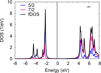
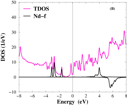
Figure 4: $f$-electron density of states (fDOS, and $j$ = 5/2, 7/2 projected) for the Nd atom in Nd@GR calculated with DFT+HIA (A); the total (TDOS) and spin-resolved $f$-orbital DOS for the Nd adatom in Nd@GR calculated with DFT+U-FLL (B).

V Conclusions

The electronic structure and magnetic properties of Sm and Nd impurities on a free-standing graphene were investigated making use of DFT+U, DFT+HIA and DFT+ED methods in order to analyze the role of the electron correlations and the spin-orbit coupling. DFT+U calculations result in non-zero local magnetic moments for both adatoms. This is expected for Nd, but not for Sm, which has a nonmagnetic $f^{6}$ ($J=0$) ground state configuration. Application of the DFT+HIA and DFT+ED methods solves this problem, and yields a nonmagnetic singlet ground state with $n_{f}=6.0$, and $J=0$ for the Sm adatom, while the degenerate ground state of Nd adatom retains the local magnetic moment with $n_{f}=3.7$, and $J=4.0$. Our results show that the DFT+U predictions for the $f$ systems close to the atomic limit should be treated with caution, keeping in mind the ambiguities inherent to the DFT+U approximation.

VI Acknowledgments

We acknowledge stimulating discussions with P. Jelínek, M. Telychko and L. Havela. Financial support was provided by the Czech Science Foundation (GACR) Grant No. 15-07172S, the National Science Centre (Poland) Grant No. DEC-2015/17/N/ST3/03790, the Deutsche Forschungsgemeinschaft (DFG) Grant No. DFG LI 1413/8-1. Access to computing and storage facilities owned by parties and projects contributing to the National Grid Infrastructure MetaCentrum provided under the programme ”Projects of Projects of Large Research, Development, and Innovations Infrastructures” (CESNET LM2015042), is appreciated.

References

- Katsnelson (2012) M. I. Katsnelson, Graphene: Carbon in Two Dimensions (Cambridge University Press, 2012).
- Eelbo et al. (2013) T. Eelbo, M. Waśniowska, P. Thakur, M. Gyamfi, B. Sachs, T. O. Wehling, S. Forti, U. Starke, C. Tieg, A. I. Lichtenstein, and R. Wiesendanger, Phys. Rev. Lett. 110, 136804 (2013).
- Sessi et al. (2014) V. Sessi, S. Stepanow, A. N. Rudenko, S. Krotzky, K. Kern, F. Hiebel, P. Mallet, J.-Y. Veuillen, O. Šipr, J. Honolka, and N. B. Brookes, New J. Phys. 16, 062001 (2014).
- Wehling et al. (2011) T. O. Wehling, A. I. Lichtenstein, and M. I. Katsnelson, Phys. Rev. B 84, 235110 (2011).
- Virgus et al. (2014) Y. Virgus, W. Purwanto, H. Krakauer, and S. Zhang, Phys. Rev. Lett. 113, 175502 (2014).
- Liu et al. (2010) X. Liu, C. Z. Wang, M. Hupalo, Y. X. Yao, M. C. Tringides, W. C. Lu, and K. M. Ho, Phys. Rev. B 82, 245408 (2010).
- Cohen et al. (2008) A. J. Cohen, P. Mori-Sanchez, and W. Yang, Science 321, 792 (2008).
- Perdew and Zunger (1981) J. P. Perdew and A. Zunger, Phys. Rev. B 23, 5048 (1981).
- Becke (1993) A. Becke, J. Chem. Phys. 98, 1372 (1993).
- Skriver (1985) H. L. Skriver, Phys. Rev. B 31, 1909 (1985).
- Liechtenstein et al. (1995) A. I. Liechtenstein, V. I. Anisimov, and J. Zaanen, Phys. Rev. B 52, R5467 (1995).
- Hewson (1993) A. Hewson, The Kondo Problem to Heavy Fermions (Cambridge University Press, 1993).
- Thunström et al. (2009) P. Thunström, I. Di Marco, A. Grechnev, S. Lebègue, M. I. Katsnelson, A. Svane, and O. Eriksson, Phys. Rev. B 79, 165104 (2009).
- Locht et al. (2016) I. L. M. Locht, Y. O. Kvashnin, D. C. M. Rodrigues, M. Pereiro, A. Bergman, L. Bergqvist, A. I. Lichtenstein, M. I. Katsnelson, A. Delin, A. B. Klautau, B. Johansson, I. Di Marco, and O. Eriksson, Phys. Rev. B 94, 085137 (2016).
- Kresse and Furthmuller (1996) G. Kresse and J. Furthmuller, Phys. Rev. B 54, 11169 (1996).
- Blochl (1994) P. E. Blochl, Phys. Rev. B 50, 17953 (1994).
- Perdew et al. (1996) J. P. Perdew, K. Burke, and M. Ernzerhof, Phys. Rev. Lett. 77, 3865 (1996).
- van der Marel and Sawatzky (1988) D. van der Marel and G. A. Sawatzky, Phys. Rev. B 37, 10674 (1988).
- Wimmer et al. (1981) E. Wimmer, H. Krakauer, M. Weinert, and A. J. Freeman, Phys. Rev. B. 24, 864 (1981).
- Shick et al. (1997) A. B. Shick, D. L. Novikov, and A. J. Freeman, Phys. Rev. B 56, R14259 (1997).
- Solovyev et al. (1998) I. V. Solovyev, A. I. Liechtenstein, and K. Terakura, Phys. Rev. Lett. 80, 5758 (1998).
- Shick et al. (1999) A. B. Shick, A. I. Liechtenstein, and W. E. Pickett, Phys. Rev. B 60, 10763 (1999).
- Anisimov et al. (1991) V. I. Anisimov, J. Zaanen, and O. K. Andersen, Phys. Rev. B 44, 943 (1991).
- Lichtenstein and Katsnelson (1998) A. I. Lichtenstein and M. I. Katsnelson, Phys. Rev. B 57, 6884 (1998).
- Kolorenc et al. (2012) J. Kolorenc, A. I. Poteryaev, and A. I. Lichtenstein, Phys. Rev. B 85, 235136 (2012).
- Kolorenč et al. (2015) J. Kolorenč, A. B. Shick, and A. I. Lichtenstein, Phys. Rev. B 92, 085125 (2015).
- Shick et al. (2009) A. B. Shick, J. Kolorenc, A. I. Lichtenstein, and L. Havela, Phys. Rev. B 80, 085106 (2009).
- Shick et al. (2006) A. B. Shick, L. Havela, J. Kolorenc, V. Drchal, T. Gouder, and P. M. Oppeneer, Phys. Rev. B 73, 104415 (2006).
- Gunnarsson et al. (1989) O. Gunnarsson, O. K. Andersen, O. Jepsen, and J. Zaanen, Phys. Rev. B 39, 1708 (1989).
- Moore and van der Laan (2009) K. Moore and G. van der Laan, Rev. Mod. Phys. 81, 235 (2009).
- Li et al. (2016) Y.-J. Li, M. Wang, M. yu Tang, X. Tian, S. Gao, Z. He, Y. Li, and T.-G. Zhou, Physica E 75, 169 (2016).
- Miyamachi et al. (2013) T. Miyamachi, T. Schuh, T. Markl, C. Bresch, T. Balashov, A. Stohr, C. Karlewski, S. Andre, M. Marthaler, M. Hoffmann, M. Geilhufe, S. Ostanin, W. Hergert, I. Mertig, G. Schon, A. Ernst, and W. Wulfhekel, Nature 503, 242 (2013).
- Donati et al. (2014) F. Donati, A. Singha, S. Stepanow, C. Wäckerlin, J. Dreiser, P. Gambardella, S. Rusponi, and H. Brune, Phys. Rev. Lett. 113, 237201 (2014).