Cosmological Perturbations in Restricted

$f(R)$-Gravity

M. Chaichian,^a A. Ghalee,^b J. Klusoň,^c,

^aDepartment of Physics, University of Helsinki,P.O. Box 64,
FI-00014 Helsinki, Finland
^bDepartment of Physics, Tafresh University, Tafresh 39518 79611, Iran
^cDepartment of Theoretical Physics and Astrophysics, Faculty of Science,
Masaryk University, Kotlářská 2, 611 37, Brno, Czech Republic

We investigate the metric perturbations of the restricted $f(R)$ theory of gravity in the cosmological context and explore the phenomenological implications of this model. We show that it is possible to construct a restricted model of gravity, in which the background equations are the same as the equations of motion which are derived from the Einstein-Hilbert action with the cosmological constant term. We argue that the deviation from the Einstein-Hilbert model emerges in the perturbed equations, for which we have a non-vanishing anisotropic stress. Further, with the help of the results of Planck data for the modified gravity we obtain constraints on the parameters of the model.

1 Introduction

Recently a new model of restricted $f(R)$-gravity has been proposed in [2]. This proposal is based on the idea of a mild breaking of the diffeomorphism invariance of the four- dimensional $f(R)$ gravity. Recall that $f(R/M^{2}_{P})$-gravity is described by the action

$$S_{f(R)}=\int d^{4}x\sqrt{-g}\left[\frac{M_{P}^{2}R}{2}+\eta M_{P}^{4}f\left(\frac{R}{M_{P}^{2}}\right)\right]+S_{Matter}\ ,$$ (1)

where $M_{P}^{2}$ is the reduced Planck mass and $\eta$ is a dimensionless constant. This action is invariant under the full four-dimensional diffeomorphism by construction. In order to find the restricted form of $f(R)$-gravity, it is useful to introduce the $3+1$-decomposition of the metric $g_{\mu\nu}$ [4, 5]

$$g_{00}=-N^{2}+N_{i}h^{ij}N_{j},\quad g_{0i}=N_{i},\quad g_{ij}=h_{ij}\ ,$$

$$g^{00}=-\frac{1}{N^{2}},\quad g^{0i}=\frac{N^{i}}{N^{2}},\quad g^{ij}=h^{ij}-\frac{N^{i}N^{j}}{N^{2}}\ ,$$ (2)

where we have defined $h^{ij}$ as the inverse of the induced metric $h_{ij}$ on the Cauchy surface $\Sigma_{t}$ at each time $t$,

$$h_{ik}h^{kj}=\delta_{i}^{\ j}$$ (3)

and we denote $N^{i}=h^{ij}N_{j}$. The four-dimensional scalar curvature in $3+1$ formalism has the form

$$R(g_{\mu\nu}) = K_{ij}\mathcal{G}^{ijkl}K_{kl}+{}^{(3)}R+\frac{2}{\sqrt{-g}}\partial_{\mu}(\sqrt{-g}n^{\mu}K)-\frac{2}{\sqrt{h}N}\partial_{i}(\sqrt{h}h^{ij}\partial_{j}N)$$

$$\equiv K_{ij}\mathcal{G}^{ijkl}K_{kl}+{}^{(3)}R+\Xi\ ,$$

where the extrinsic curvature of the spatial hypersurface $\Sigma_{t}$ at the time $t$ is defined as

$$K_{ij}=\frac{1}{2N}\left(\frac{\partial h_{ij}}{\partial t}-D_{i}N_{j}-D_{j}N_{i}\right),$$ (5)

with $D_{i}$ being the covariant derivative determined by the metric $h_{ij}$, and where the de Witt metric is defined as

$$\mathcal{G}^{ijkl}=\frac{1}{2}(h^{ik}h^{jl}+h^{il}h^{jk})-h^{ij}h^{kl}$$ (6)

with inverse

$$\mathcal{G}_{ijkl}=\frac{1}{2}(h_{ik}h_{jl}+h_{il}h_{jk})-\frac{1}{2}h_{ij}h_{kl}\$$ (7)

which obeys the relation

$$\mathcal{G}_{ijkl}\mathcal{G}^{klmn}=\frac{1}{2}(\delta_{i}^{m}\delta_{j}^{n}+\delta_{i}^{n}\delta_{j}^{m})\ .$$ (8)

Further, $n^{\mu}$ is the future-pointing unit normal vector to the hypersurface $\Sigma_{t}$, which is written in terms of the ADM variables as

$$n^{0}=\sqrt{-g^{00}}=\frac{1}{N},\quad n^{i}=-\frac{g^{0i}}{\sqrt{-g^{00}}}=-\frac{N^{i}}{N}\ .$$ (9)

In order to formulate the restricted $f(R)$-gravity we break the full diffeomorphism invariance of the $f(R)$-gravity by performing the replacement

$$R\rightarrow R+(\Upsilon-1)\Xi\ ,$$ (10)

where $\Upsilon$ is a dimensionless parameter that controls the breaking of the diffeomorphism invariance of the action. Even if the shift (10) seems to be very mild, it turns out that it has significant impact on the Hamiltonian structure of this theory as was shown in [2]. Careful analysis performed there showed that in order to have a consistent theory from the Hamiltonian analysis point of view, it is necessary to include terms which depend on the spatial derivative of the lapse $a_{i}=\frac{\partial_{i}N}{N}$ into the action. Further, the breaking of the diffeomorphism invariance suggests the possibility to define theory with the generalized de Witt metric [6, 7]

$$\tilde{\mathcal{G}}^{ijkl} = \frac{1}{2}(h^{ik}h^{jl}+h^{il}h^{jk})-\lambda h^{ij}h^{kl}\ ,\quad\lambda\neq\frac{1}{3}\ ,$$

$$\tilde{\mathcal{G}}_{ijkl} = \frac{1}{2}(h_{ik}h_{jl}+h_{il}h_{jk})-\frac{\lambda}{3\lambda-1}h_{ij}h_{kl}\ .$$

In summary, we proposed in [2] the extended form of the restricted $f(R)$-gravity when we performed the replacement

$$R\rightarrow R_{\Upsilon}\equiv K_{ij}\tilde{\mathcal{G}}^{ijkl}K_{kl}+{}^{(3)}R+\Upsilon\Xi+\gamma_{1}a_{i}a^{i}+\gamma_{2}{}^{(3)}R^{ij}a_{i}a_{j}\ ,$$ (12)

where $\gamma_{1},\gamma_{2}$ are the corresponding coupling constants. We showed there that this theory is consistent from the Hamiltonian analysis point of view since the structure of constraints is the same as in case of non-projectable Hořava-Lifshitz gravity [8, 9, 10], for the Hamiltonian analysis, see [11, 12, 13, 14] and also [15, 16, 17, 18, 19, 20]. We also analyzed cosmological solutions of the restricted $f(R)$-gravity and we found new solutions whose properties depend on the value of the parameter $\Upsilon$. It is important to emphasize that some of these solutions cannot be found in the diffeomorphism invariant $f(R)$-gravity.

Due to the fact that there are new cosmological solutions, it is natural to investigate them in more details. The aim of this paper is to focus on the analysis of the cosmological fluctuations of the restricted $f(R)$-gravity. As the first step we determine the background equations from the restricted $f(R)$-gravity action when we focus on i a time-dependent ansatz. Then we analyze the fluctuations above this background. Due to the fact that the scalar, vector and tensor fluctuations decouple at the quadratic order we can analyze each kind of the fluctuations separately. We show that the restricted $f(R)$-gravity differs from the standard $f(R)$-gravity in the scalar sector, while the vector and tensor sectors have the same properties as in the case of diffeomorphism invariant $f(R)$-gravity. More precisely, we show that with suitable choice of parameters the restricted $f(R)$-gravity allows to explain recent observation data that predict the possibility of the existence of a non-zero anisotropic stress (See for example [25].).

This paper is organized as follows. In the next section (2) we briefly review the equations of motion of the restricted $f(R)$-gravity evaluated on the time-dependent cosmological solution. In section (3) we analyze the fluctuations above this background and in section (4) we discuss our results with relation to the recent phenomenological observations. Finally, in conclusion (5) we outline our results.

2 Background Equations

In this section we derive the equations of motion for the restricted $f(R)$-gravity when we presume the Friedmann-Robertson-Walker (FRW) form of the background. Recall that the restricted $f(R/M^{2}_{P})$-gravity action has the form

$$S_{res}=\int d^{4}x\sqrt{-g}\left[M_{P}^{2}\frac{R_{\Upsilon}}{2}+\eta M_{P}^{4}f\big{(}\frac{R_{\Upsilon}}{M_{P}^{2}})\right]+S_{Matter}\ ,$$ (13)

where $R_{\Upsilon}$ is defined in (12). The matter part contributes to the gravitational equations of motion through the stress-energy tensor which is defined as

$$T_{\mu\nu}=-\frac{2}{\sqrt{-g}}\frac{\delta S_{Matter}}{\delta g^{\mu\nu}}\ .$$ (14)

Our goal is to analyze the spatially homogeneous and isotropic Universe so that the metric ansatz is the FRW metric which has the form

$$ds^{2}=-N(t)^{2}dt^{2}+a(t)^{2}dx^{i}dx^{j}\delta_{ij}\ ,$$ (15)

where $N=N(t)$ is the lapse and $a=a(t)$ is the scale factor. As usual, the Hubble parameter is defined as $H\equiv\dot{a}/a$. Note that we cannot set $N(t)=1$ from the beginning due to the restricted form of the diffeomorphism. But, since for the background equations all quantities depend only on time, one can use redefinition of time in (15) to set $N=1$ in the background equations. We also presume matter in the form of a prefect fluid which means that the stress-energy tensor has the form

$$T^{\alpha}_{\ \beta}=\left(\begin{array}[]{cccc}-\rho(t)&0&0&0\\ 0&p(t)&0&0\\ 0&0&p(t)&0\\ 0&0&0&p(t)\\ \end{array}\right)\ .$$ (16)

Since we presume that the full diffeomorphism is broken in the gravitational sector only we find that the matter action is diffeomorphism invariant. As a result the stress-energy tensor is conserved in the sense $\nabla_{\mu}T^{\mu\nu}=0$ on the condition that the matter satisfies the equation of motion. Now for the background (15) we obtain

$$\Gamma^{0}_{00}=\frac{\dot{N}}{N}\ ,\quad\Gamma^{0}_{ij}=\frac{1}{N^{2}}\dot{a}a\delta_{ij}\ ,\quad\Gamma^{0}_{0i}=0\ ,\quad\Gamma^{i}_{00}=0\ ,\quad\Gamma^{i}_{j0}=\delta^{i}_{j}H\ ,\quad\Gamma^{i}_{jk}=0\$$

so that the conservation of the stress-energy tensor implies the standard conservation equation

$$\dot{\rho}+3H(\rho+p)=0\ .$$

Using (15) and the general relations in the ADM formalism, which are discussed in Ref. [5], one can show that

$$\Xi=-6\frac{H\dot{N}}{N^{3}}+6\frac{\dot{H}}{N^{2}}+18\frac{H^{2}}{N^{2}}\hskip 2.27626pt.$$ (19)

The generalized Friedmman equation for the model has been determined in [2] as

$$3AH^{2}+\eta M_{P}^{2}f+\eta(6AH^{2}-R_{\Upsilon})F+6\eta\Upsilon H\dot{F}=\frac{\rho}{M_{P}^{2}}\ ,$$ (20)

where

$$R_{\Upsilon}=-6AH^{2}+\Upsilon(6\dot{H}+18H^{2}),\hskip 4.26773ptf\equiv f\big{(}\frac{R_{\Upsilon}}{M_{P}^{2}}\big{)}\hskip 4.26773pt,F\equiv M_{P}^{2}\frac{df}{dR_{\Upsilon}}\equiv f^{\prime}\hskip 4.26773pt,A\equiv\frac{3\lambda-1}{2}\ .$$ (21)

Note that we have defined prime as derivative with respect to the argument of $f$. As a result, $F,f^{\prime\prime},...$ are dimensionless quantities. Finally, we note that there is still another equation after performing the time derivative of eq. (20) and then use eq. (19)

$$A\dot{H}(1+2\eta F)+\eta H(2A-3\Upsilon)\dot{F}+\Upsilon\eta\ddot{F}=-\frac{(\rho+p)}{2M_{P}^{2}}\ .$$ (22)

After this brief review of the background equations we now switch to the main topic of this paper which is the analysis of the cosmological perturbations.

3 Cosmological Perturbations

The goal of this section is to derive equations for the perturbed FRW space-time in the Arnowitt-Deser-Misner(ADM) formalism . As a check of the validity of our approach, we note that for $\Upsilon=1,\lambda=1,\gamma_{1}$ and $\gamma_{2}=0$ the results derived in this paper should reduce to the corresponding results of the standard $f(R/M_{P}^{2})$ gravity, see for example the review [3].

To begin with, we emphasize that we are writing our equations in the Newtonian gauge which is defined by $N^{i}=0$. We use the Newtonian gauge for the following reason: As it has been argued in [23], one of the advantages of the Newtonian gauge is that the physical fields which are defined by the gauge fixing, coincide with the gauge-invariant variables. Note also that it is an easy task to move from the Newtonian gauge to other gauges [23]. Finally, note that due to the fact that the spatial section of the metric (15) is flat, it is natural to use the Fourier decomposition of the perturbation where the Fourier components of a general perturbation $U(t,\textbf{x})$ are defined as

$$U_{k}(t)=\int d^{3}\mathbf{x}U(t,\textbf{x})e^{-i\textbf{k.x}}\ ,$$ (23)

where $\mathbf{x}=(x^{1},x^{2},x^{3}),\mathbf{k}=(k^{1},k^{2},k^{3})$. Further, we also decompose $F$ and $\dot{F}$ into the homogeneous and perturbed parts as

$$F=\bar{F}+\delta F,\hskip 4.26773pt\dot{F}=\dot{\bar{F}}+\dot{\delta F}\ ,$$ (24)

where $\hskip 2.84544pt\bar{}\hskip 2.84544pt$ over any quantity shows the unperturbed part of that quantity. In the case of the fluctuations of the matter we use the following parameterization for the perturbed energy-momentum tensor

$$\delta T_{0}^{0}=-\delta\rho,\hskip 2.84544pt\delta T_{0}^{i}=-(\rho+p)\partial_{i}v,\hskip 2.84544pt\delta T_{i}^{j}=\delta p\delta_{i}^{j}\ ,$$ (25)

where $v$ is the potential for the spatial velocity of the fluid.

3.1 The Scalar Metric Perturbations

Before we proceed to the study of the perturbed equations it is instructive to discuss the role of diffeomorphism symmetry in the cosmological context.
For a full diffeomorphism invariant model, as for example the Einstein-Hilbert action or $f(R)$gravity action, there is no a priori preferred coordinate system. Of course the symmetry can be broken by imposing other restrictions on the model. For example, in the cosmological context, it has been shown that the only coordinate system(observer) that is compatible with the assumption of homogeneity and isotropy of space is described by the FRW metric [22]. The uniqueness of FRW metric helps us to choose it as the background metric for our model in this paper. But, the uniqueness of the metric is broken if we consider Universe which is not homogeneous. The deviation from homogeneity is considered as the perturbed FRW metric. For example, the scalar metric perturbations can be parameterized as [23]

$$ds^{2}=-(1+2Y)dt^{2}+2a\partial_{i}Bdx^{i}dt+a^{2}[(1+2\zeta)\delta_{ij}+2\partial_{i}\partial_{j}E]dx^{i}dx^{j}\ ,$$ (26)

where $Y=Y(t,\mathbf{x})$,$B=B(t,\mathbf{x})$, $E=E(t,\mathbf{x})$, $\zeta=\zeta(t,\mathbf{x})$ are $3-$scalars.
It is an unnecessary and senseless task to insert the above expression into general equations of motion in order to obtain the equations of motion for these $3-$scalars. The reason for this statement is that, similar to the model with the full diffeomorphism symmetry, here we confront with the so-called gauge problem. The problem arises when we note that the model is invariant under the coordinate transformation as $t\rightarrow t+P(t)$, $x^{i}\rightarrow x^{i}+\partial^{i}K(t,\mathbf{x})$, where $\partial^{i}=\delta^{ij}\partial_{j}$. Under this transformation the components of the metric (26) transform as [23]

$$Y\rightarrow Y^{t} = Y-\dot{P}(t)\ ,$$

$$B\rightarrow B^{t} = B+\frac{P(t)}{a}-a\dot{K}(t,\mathbf{x})\ ,$$

$$E\rightarrow E^{t} = E-K(t,\mathbf{x})\ ,$$

$$\zeta\rightarrow\zeta^{t} = \zeta-HP(t)\ .$$

Therefore, even if we tried to obtain the equations for the components of eq.(26), we would have some solutions which are unphysical in the sense that they can be derived by application of the transformation (3.1) on some particular solutions. In order to avoid the above problem, i.e. the gauge problem, one can choose a specific gauge (coordinate) or use the gauge-invariant quantities. In the process of the gauge fixing, values for $P(t)$ and $K(t,\mathbf{x})$ are explicitly specified such that we have not any residual symmetry for the solution. Physically, gauge fixing means that a specific spatial coordinate has been chosen.
In the following we will work with the Newtonian gauge. The Newtonian gauge is defined as the perturbed metric for observers who are immobile at the hypersurfaces of constant time. Also, the normal vector of the hypersurfaces are the same as the worldlines of the observers at any time. Thus, the Newtonian gauge is described by [23]

$$ds^{2}=-(1+2Y)dt^{2}+a^{2}[(1+2\zeta)\delta_{ij}]dx^{i}dx^{j}\ .$$ (28)

The Newtonian gauge is the preferred gauge for the late-time cosmology as was argued in [24]. Therefore, we will use it to compare the results of our model with the Plank observations. Finally we should emphasize that it is still possible to construct the gauge invariant quantities form the Newtonian gauge variables [23].
To proceed further, we note that it is convenient to parameterize the scalar metric perturbations in the Newtonian gauge as

$$N^{2}=1+2Y\equiv e^{2\Phi},\hskip 4.26773pth_{ij}=a^{2}(1+2\zeta)\delta_{ij}\equiv a^{2}e^{-2\Psi}\delta_{ij}\ ,$$ (29)

where $\Phi$ and $\Psi$ are space and time dependent. Using these definitions in (12) we easily find

$$\begin{split}R_{\Upsilon}|_{scalar}=&{}^{3}R+6(3\Upsilon-A)e^{-2\Phi}(H-\dot{\Psi})^{2}+6\Upsilon e^{-2\Phi}(\dot{H}-\ddot{\Psi})\\ &-6\Upsilon\dot{\Phi}e^{-2\Phi}(H-\dot{\Psi})-2\Upsilon\frac{e^{2\Psi}}{a^{2}}\partial^{2}\Phi\\ &+2\Upsilon\frac{e^{2\Psi}}{a^{2}}\partial_{i}\Phi\partial_{i}\Psi+(\gamma_{1}-2\Upsilon)\frac{e^{2\Psi}}{a^{2}}\partial_{i}\Phi\partial_{i}\Phi\ .\end{split}$$ (30)

As a check, we note that for $\Phi=\Psi=0$ the above relation reduces to the background form of $R_{\Upsilon}$ given in eq.(21). Now by performing the linearization of the expression (30), we obtain Fourier component of $\delta R_{\Upsilon}|_{scalar}$

$$\begin{split}\delta R_{\Upsilon}|_{scalar}(k)=&\frac{-4k^{2}}{a^{2}}\Psi+\frac{2\Upsilon k^{2}}{a^{2}}\Phi-12(3\Upsilon-A)H^{2}\Phi\\ &-12\Upsilon\dot{H}\Phi-6\Upsilon H\dot{\Phi}-6\Upsilon\ddot{\Psi}-12(3\Upsilon-1)H\dot{\Psi}\ ,\end{split}$$ (31)

where $k^{2}\equiv k_{i}k^{i}$. Further, inserting (25) and (29) into the equation (2) and by performing the corresponding linearization, we obtain two equations

$$\dot{\delta\rho}+3H(\delta\rho+\delta p)=\frac{k^{2}}{a^{2}}\delta q+3(\rho+p)\dot{\Psi}\ ,$$ (32)

and

$$\dot{\delta q}+3H\delta q+\delta p+(\rho+p){\Phi}=0\ ,$$ (33)

where $\delta q\equiv-(\rho+p)v$. Note that these equations have the same forms as the corresponding equations for the usual $f(R/M^{2})$ gravity. In order to derive the remaining equations, we proceed in the following way. To begin with, we insert (30) into the action. As we pointed out we work in the Newtonian gauge. Then in order to vary the action with respect to the shift, it is sufficient to consider the terms which are proportional to $N_{i}\Psi$ and $N_{i}\Phi$. For example, if we define $\delta_{N_{i}}$ as a variation with respect to the shift then for $S_{Matter}$ we obtain

$$\delta_{N_{i}}S_{Matter}=-\frac{1}{2}\int d^{4}x\sqrt{-g}T^{\mu\nu}\delta_{N_{i}}g_{\mu\nu}=-\frac{1}{2}\int d^{4}xa^{3}T^{0i}\delta N_{i}+\mathcal{O}(N_{i}^{2})\ .$$ (34)

Using this result and also using the following relations

$$n^{\mu}=\big{(}e^{-\Phi},-N^{i}e^{-\Phi}\big{)},\hskip 2.84544pt\Gamma^{i}_{ij}=-3\partial_{j}\Psi$$ (35)

and after some integration by parts we obtain

$$\begin{split}S=&-AM_{P}^{2}\int d^{4}x2a[H\Phi+\dot{\Psi}]\partial_{i}N_{i}(1+2\eta\bar{F})-4A\eta M_{P}^{2}\int d^{4}xaHN_{i}\partial_{i}\delta F\\ &-2\eta\Upsilon M_{P}^{2}\int d^{4}xa[N_{i}\partial_{i}\dot{\delta F}-\partial_{i}\Phi N_{i}\dot{\bar{F}}-3HN_{i}\partial_{i}\delta F]+S_{Matter}\ .\end{split}$$ (36)

Further on, performing the variation with respect to $N_{i}$ and using the Fourier components of the perturbations we obtain

$$A(H\Phi+\dot{\Psi})(1+2\eta\bar{F})=\eta\big{[}\Upsilon\dot{\delta F}-\Upsilon\Phi\dot{\bar{F}}+(2A-3\Upsilon)H\delta F\big{]}-\frac{1}{2M_{P}^{2}}\delta q\ .$$ (37)

In case of the variation of the action with respect to $\Phi$ we set $N_{i}=0$ in the action and then expand the action up to the second order in $\Phi$ and $\Psi$. This procedure, after some integration be parts and using Eq. (20), leads to

$$\begin{split}\delta_{\Phi}S_{res}=\int d^{4}xa^{3}M_{P}^{2}\delta\Phi\Big{[}&\Big{(}-12A\Phi H^{2}+\frac{4}{a^{2}}\partial^{2}\Psi-12AH\dot{\Psi}-\frac{2\gamma_{1}}{a^{2}}\partial^{2}\Phi\Big{)}\times\\ &\times\Big{(}\frac{1}{2}+\eta\bar{F}\Big{)}+\eta\big{(}(12A-18\Upsilon)H^{2}-6\Upsilon\dot{H}-\frac{2\Upsilon}{a^{2}}\partial^{2}\big{)}\delta F\\ &-\eta\dot{\bar{F}}\big{(}12\Upsilon H\Phi+6\Upsilon\dot{\Psi}\big{)}+6\eta\Upsilon H\dot{\delta F}-\delta_{\Phi}S_{Matter}\Big{]}\ \end{split}$$ (38)

so that we easily find the Fourier form of the equation of motion for $\Phi$

$$\begin{split}&\eta\big{[}(6A-9\Upsilon)H^{2}-3\Upsilon\dot{H}+\frac{\Upsilon}{a^{2}}k^{2}\big{]}\delta F-3\Upsilon\eta\dot{\bar{F}}(2H\Phi+\dot{\Psi})\\ &+3\eta\Upsilon H\dot{\delta F}-\frac{\delta\rho}{2M_{P}^{2}}=(3A\Phi H^{2}+\frac{k^{2}}{a^{2}}\Psi+3AH\dot{\Psi}-\gamma_{1}\frac{k^{2}}{2a^{2}}\Phi)(1+2\eta\bar{F})\ .\end{split}$$ (39)

For reasons that will become clear later we derive $\delta p$ in two different ways. In the first case we use (32) and (39). Then in order to eliminate $(\rho+p)$ in these formula, we use (22). Collecting these pieces together we obtain an equation

$$\begin{split}\frac{\delta p}{2M_{P}^{2}}=&\eta(2A\dot{\Psi}+4AH\Phi+\Upsilon\dot{\Phi}-\gamma_{1}\frac{k^{2}}{3Ha^{2}}\Phi)\dot{\bar{F}}-2\eta H\dot{\delta F}+2\eta\Upsilon\Phi\ddot{\bar{F}}-\eta\Upsilon\ddot{\delta F}\\ &+\eta\big{[}(3\Upsilon-2A)\dot{H}+(9\Upsilon-6A)H^{2}+\frac{2k^{2}}{3a^{2}}(A-2\Upsilon)\big{]}\delta F\\ &+\big{[}\dot{\Phi}H+2A\dot{H}\Phi+A\ddot{\Psi}+3A\Phi H^{2}+3AH\dot{\Psi}+\frac{k^{2}}{3a^{2}}(\Psi-A\Phi)\\ &\hskip 4.26773pt+(1-A)\frac{k^{2}}{3Ha^{2}}\dot{\Psi}-\gamma_{1}\frac{k^{2}}{6a^{2}}(\frac{\dot{\Phi}}{H\Phi}+1)\Phi\big{]}(1+2\eta\bar{F})\ ,\end{split}$$ (40)

where we also used the fact that $\dot{R}_{\Upsilon}\delta F=\delta R_{\Upsilon}\dot{\bar{F}}$.
The second way how to derive the relation for $\delta p$ is to use eqs. (33),(37). We again use eq.(22) in order to eliminate $(\rho+p)$, so that we obtain

$$\begin{split}\frac{\delta p}{2M_{P}^{2}}=&\eta[2\dot{\Psi}+2(1+A)H\Phi+\Upsilon\dot{\Phi}]\dot{\bar{F}}-2\eta AH\dot{\delta F}+2\eta\Upsilon\Phi\ddot{\bar{F}}-\eta\Upsilon\ddot{\delta F}\\ &+\eta\big{[}(3\Upsilon-2A)\dot{H}+(9\Upsilon-6A)H^{2}\big{]}\delta F\\ &+\big{[}\dot{\Phi}H+2\dot{H}\Phi+\ddot{\Psi}+3\Phi H^{2}+3H\dot{\Psi}\big{]}(1+2\eta\bar{F})\ .\end{split}$$ (41)

The right-hand side of eqs. (40) and (41) are the same if

$$\begin{split}&\Big{[}(1-A)\dot{\Phi}H+(1-A)\frac{k^{2}}{3Ha^{2}}\dot{\Psi}+\frac{k^{2}}{3a^{2}}(\Psi-A\Phi)-\frac{\gamma_{1}k^{2}}{6a^{2}}(\frac{\dot{\Phi}}{H\Phi}+1)\Phi\Big{]}\Big{[}1+2\eta\bar{F}\Big{]}\\ &=2\eta\frac{k^{2}}{3a^{2}}(2\Upsilon-A)\delta F+\eta\Big{[}2(1-A)H\Phi+2(1-A)\dot{\Psi}+\gamma_{1}\frac{k^{2}}{3Ha^{2}}\Phi\Big{]}\dot{\bar{F}}\ .\end{split}$$ (42)

As is clear, the equations are simplified by taking $\lambda=1$, which results in $A=1$. As a check, note that for $\Upsilon=1,\lambda=1$ and $\gamma_{1}=0$ these equations match the corresponding relations for the usual $f(R/M_{P}^{2})$ gravity.

3.2 Tensor Metric Perturbations

In this section we focus on the metric tensor perturbations $\gamma_{ij}$. Recall that the perturbed line element has the form

$$ds^{2}=-dt^{2}+a^{2}[\delta_{ij}+\gamma_{ij}]dx^{i}dx^{j},$$ (43)

where $\partial_{i}\gamma_{ij}=\gamma_{i}^{i}=0$. In order to derive equations in this sector we use the fact that $\sqrt{-g}$ does not contain the metric tensor perturbations up to the second order. Further, using the traceless condition on $\gamma_{ij}$ it is easy to show that the metric perturbations do not appear in $K$. Thus, it turns out that the terms in (12) which are proportional to $\Upsilon$ and $\lambda$ do not contribute to the metric tensor perturbations. As a result the analysis of this sector is very similar to the analysis of tensor fluctuations in standard $f(R)$ gravity. Explicitly, the second order action for these modes has the form

$$\delta S|_{tensor}=\frac{M_{P}^{2}}{8}\int d^{4}x[1+2\eta\bar{F}]\big{[}a\gamma_{ij}\partial^{2}\gamma_{ij}+a^{3}\dot{\gamma}_{ij}^{2}\big{]}\ .$$ (44)

Then in order to avoid the ghost instability we must impose the following condition

$$1+2\eta\bar{F}>0.$$ (45)

Performing variation of (44) with respect to $\gamma_{ij}$ and using the following Fourier representation

$$\gamma_{ij}=\int\frac{d^{3}k}{(2\pi)^{3/2}}\sum_{s=\pm}\epsilon_{ij}^{s}(k)\gamma_{k}^{s}(t)e^{i\overrightarrow{k}.\overrightarrow{x}}\ ,$$ (46)

where $\epsilon_{ii}=k^{i}\epsilon_{ij}=0$ and $\epsilon_{ij}^{s}(k)\epsilon_{ij}^{{s^{\prime}}}(k)=2\delta_{ss^{\prime}}$, leads to the second order differential equation for $\gamma^{s}_{k}$

$$\ddot{\gamma_{k}^{s}}+\dot{\gamma_{k}^{s}}\frac{d}{dt}\ln[a^{3}(1+2\eta\bar{F})]+(\frac{k}{a})^{2}\gamma_{k}^{s}=0$$ (47)

which has the same form as in the standard $f(R)$-gravity.

3.3 Vector Metric Perturbations

In this section we perform an analysis of vector metric perturbations. As in the case of the prefect fluid we consider the following form of the perturbed stress-tensor in the vector sector

$$\delta T^{0}_{i}|_{vector}=\delta q_{i}^{V}\ .$$ (48)

Then from $\nabla_{\mu}T^{\mu\nu}=0$ it follows that

$$\dot{\delta q_{i}^{V}}+3H\delta q_{i}^{V}=0\ .$$ (49)

As in case of the metric perturbations the favorite gauge in this sector is the so-called vector gauge which is defined by

$$ds^{2}=-dt^{2}+2aS_{i}dx^{i}dt+a^{2}\delta_{ij}dx^{i}dx^{j}\ ,$$ (50)

where $\partial_{i}S_{i}=0$. Again, from the above definition and the condition on $S_{i}$ it turns out that the terms in (13) which are proportional to $\Upsilon$ do not contribute in this sector. Then the second order action takes the following form

$$\delta S|_{vector}=-\frac{M_{P}^{2}}{2}\int d^{4}xaS_{i}\partial^{2}S_{i}(1+2\eta\bar{F})-2\int d^{4}xa^{2}S_{i}\delta q_{i}^{V}\ .$$ (51)

Then it is easy to see that the equation for $S_{i}$ in the Fourier space has the form

$$M_{P}^{2}k^{2}(1+2\eta\bar{F})\frac{S_{i}}{a}=2\delta q_{i}^{V}$$ (52)

which coincides with the equation for the vector perturbation in the standard $f(R)$-gravity.

4 Some Phenomenological Implications

In this section we explore some phenomenological implications of our results. In this section we take $A=1$ that corresponds to $\lambda=1$. Note that this is a natural presumption, since it is expected that $\lambda$ should approach to $1$ in the low energy regime [6, 7]. It is important to emphasize that the Einstein-Hilbert gravity predicts $\Phi=\Psi$. In the more general case when $\Phi\neq\Psi$, it is useful to define an anisotropic stress, $\delta\Sigma$ as

$$\Psi-\Phi=8\pi Ga^{2}\delta\Sigma\ .$$ (53)

Clearly a non-vanishing anisotropic stress is the signature of modification of general relativity [24, 25]. Further, it is also convenient to define

$$\gamma\equiv\frac{\Psi}{\Phi}\ ,$$ (54)

so that the Einstein-Hilbert gravity predicts $\gamma=1$.
But, from the Planck CMB temperature data, the current value for $\gamma$ reported as [24]

$$\gamma_{0}-1=0.70\pm 0.94$$ (55)

which is shown by yellow and gray colors in Fig. 1. On the other hand if we consider the weak lensing data, we have [24]

$$\gamma_{0}-1=1.36_{-0.69}^{+1.0}$$ (56)

which is shown by the gray and blue colors in Fig. 1.
Let us now return to our model and consider the late-time cosmology when we can neglect the radiation and the cold dark matter. Explicitly, we consider two cases:

• Case I: In this case we presume that the cosmological constant $\Lambda$ is non-zero while $\eta=0$.
  The energy density of the cosmological constant is $\rho=\Lambda M_{P}^{2}$ so that (20) implies

  $$H^{2}=\frac{\Lambda}{3}\ .$$ (57)

  Note that this result is the same as in the case of Einstein-Hilbert gravity with the cosmological constant.
  Since for the cosmological constant we have $\delta q=\delta p=\delta\rho=0$, from eqs. (37) and (42) we have

  $$\dot{\Psi}+H\Phi=0\ ,$$ (58a)

  $$\Psi-\Phi=\frac{\gamma_{1}}{2}(\frac{\dot{\Phi}}{H\Phi}+1)\Phi\ .$$ (58b)

  If we combine these two equations together, we obtain

  $$\ddot{\Psi}+\left(\frac{2}{\gamma_{1}}+1\right)H\dot{\Psi}+\frac{2}{\gamma_{1}}H^{2}\Psi=0$$ (59)

  that has solution

  $$\Psi =C_{1}e^{-Ht}+C_{2}e^{-\frac{2}{\gamma_{1}}Ht}\hskip 11.38092pt(\text{for}\ \gamma_{1}\neq 2)\ ,$$ (60)

  $$\Psi =C_{1}e^{-Ht}+C_{2}Hte^{-Ht}\hskip 8.5359pt(\text{for}\ \gamma_{1}=2)\ ,$$ (61)

  where $C_{1}$ and $C_{2}$ are arbitrary constants. It is clear that in order to avoid instability we have to require that $\gamma_{1}>0$.
  Using now eqs. (54), (58) and (60), we obtain

  $$\gamma-1=\frac{\gamma_{1}}{2}\Big{[}1-\frac{C_{1}e^{-Ht}+C_{2}\frac{4}{\gamma_{1}^{2}}e^{-\frac{2}{\gamma_{1}}Ht}}{C_{1}e^{-Ht}+C_{2}\frac{2}{\gamma_{1}}e^{-\frac{2}{\gamma_{1}}Ht}}\Big{]}\ (\hskip 5.69046pt\text{for}\ \gamma_{1}\neq 2)$$ (62)

  and

  $$\gamma-1=\frac{C_{2}}{C_{1}-C_{2}+C_{2}Ht}\ (\hskip 5.69046pt\text{for}\ \gamma_{1}=2)\ .$$ (63)

  For the present Universe we have $H_{0}t_{0}\approx 1$ and it is easy to see that we can choose the parameters in the above equations to obtain a consistent result with the reported data for $\gamma_{0}-1$. Note also that the above relations show that if we take $t\rightarrow\infty$, we have

  $$\gamma\rightarrow 1\ ,\quad\text{if}\hskip 5.69046pt\gamma_{1}\leq 2\ ,$$

  $$\gamma\rightarrow\frac{\gamma_{1}}{2}\ ,\quad\text{if}\hskip 5.69046pt\gamma_{1}>2\ .$$

• Case II: In the second case, we neglect the cosmological constant but $\eta\neq 0$ so that we have only two independent equations which determine $\Phi$ and $\Psi$. One of these equations is obtained by multiplying eq.(37) with $3H$ and then using the corresponding result to eliminate some terms in eq.(39). This procedure gives the following equation(for $A=1$)

  $$\big{[}\frac{2k^{2}}{a^{2}}\Psi-\gamma_{1}\frac{k^{2}}{a^{2}}\Phi\big{]}(1+2\eta\bar{F})=-6\eta\Upsilon[\dot{\Psi}+H\Phi]\dot{\bar{F}}+6\eta\Upsilon(\frac{k^{2}}{3a^{2}}-\dot{H})\delta F\ .$$ (65)

  Further, eq.(42) takes the following form for $A=1$

  $$\big{[}(\Psi-\Phi)-\frac{\gamma_{1}}{2}(\frac{\dot{\Phi}}{H\Phi}+1)\Phi\big{]}\big{[}1+2\eta\bar{F}\big{]}\\ =2\eta(2\Upsilon-1)\delta F+\frac{\eta\gamma_{1}}{H}\Phi\dot{\bar{F}}.$$ (66)

  In the de Sitter space, which is a very good approximation for the late-time cosmology, eqs.(65) and (66) simplify considerably

  $$\big{[}2\Psi-\gamma_{1}\Phi\big{]}(1+2\eta\bar{F})=2\eta\Upsilon\delta F$$ (67)

  and

  $$\big{[}(\Psi-\Phi)-\frac{\gamma_{1}}{2}(\frac{\dot{\Phi}}{H\Phi}+1)\Phi\big{]}\big{[}1+2\eta\bar{F}\big{]}\\ =2\eta(2\Upsilon-1)\delta F.$$ (68)

  If we combine these two equations, we obtain the following results

  $$2(3\Upsilon-2)\Psi =\Upsilon\gamma_{1}(3-\frac{\dot{\Phi}}{H\Phi})\Phi-2(\Upsilon+\gamma_{1})\Phi\hskip 11.38092pt\left(\text{for}\ \Upsilon\neq 0,\Upsilon\neq\frac{1}{2}\right)\ ,$$ (69a)

  $$\Psi =\frac{\gamma_{1}}{2}\Phi\hskip 11.38092pt(\text{for}\Upsilon=0)\ ,$$ (69b)

  $$(\Psi-\Phi) =\frac{\gamma_{1}}{2}\left(\frac{\dot{\Phi}}{H\Phi}+1\right)\Phi\ ,\hskip 11.38092pt\left(\text{for}\Upsilon=\frac{1}{2}\right)\ .$$ (69c)

  Note that for $\Upsilon=2/3$, the first equation implies

  $$\frac{\dot{\Phi}}{H\Phi}=-\frac{2}{\gamma_{1}}.\hskip 11.38092pt\left(\text{for}\Upsilon=\frac{2}{3}\right)\ .$$ (70)

  

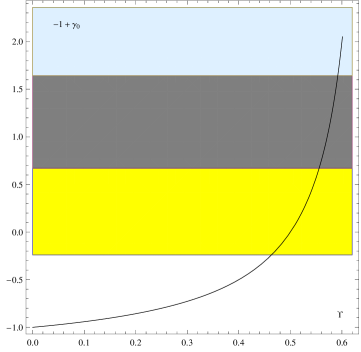
  Figure 1: Space of parameters ($\gamma_{0}-1$,$\Upsilon$) for the model. The yellow and gray regions show the values for $\gamma_{0}-1$ from the Planck CMB temperature data [24]. The gray and blue regions show the values for $\gamma_{0}-1$ from the combination of the Planck CMB temperature data and the weak lensing [24]. Solid line represents the prediction of the model in the de Sitter space for $\gamma_{1}\ll 1$.

  Finally when we insert (69) and (70) into eq. (67) or eq. (68), we obtain the equations for the remaining variables that can be easily solved. Equations (69) are interesting results since they give a relation between the parameters of the model and observation. If we take $\gamma_{1}\ll 1$ limit, it follows that

  $$(3\Upsilon-2)\Psi \approx-\Upsilon\Phi\hskip 11.38092pt\left(\text{for}\ \Upsilon\neq 0,\frac{1}{2},\frac{2}{3}\right)\ ,$$ (71a)

  $$\frac{\Psi}{\Phi} \ll 1\hskip 11.38092pt(\text{for}\ \Upsilon=0)\ ,$$ (71b)

  $$\frac{\Psi}{\Phi} \approx 1\hskip 11.38092pt\left(\text{for}\ \Upsilon=\frac{1}{2}\right)\ .$$ (71c)

  Note that, except for $\Upsilon=2/3$, in this limit( i.e $\gamma_{1}\ll 1$) the above relations do not depend on the form and dynamics of $f$ in the action (13). As shown in Fig. 1, for $\gamma_{1}\ll 1$ one can choose $\Upsilon$ to reconcile the model with the current observations.

5 Conclusion

This short note is devoted to the analysis of the cosmological fluctuations of the restricted $f(R)$-theory of gravity. We have determined the background equations of motion and then we have carefully analyzed the fluctuations above this background solution. We show that the vector and tensor fluctuations have the same dynamics as in case of the standard $f(R)$-gravity while the scalar sector possesses new interesting possibilities which depend on the values of coupling constants. In more details, we show that it is possible to choose the values of these parameters so that the predictions of the restricted $f(R)$-gravity are in agreement with recent observation data. In fact, we showed previously in [2] that the cosmological solutions found in the restricted $f(R)$-gravity are in agreement with observation and our current analysis of fluctuations confirms this fact as well. This is by itself an interesting result that suggests that it is indeed plausible to consider theories with the restricted diffeomorphism invariance as interesting alternatives to the fully diffeomorphism invariant theories of gravity.

Acknowledgement:

The work of J.K. was supported by the Grant Agency of the Czech Republic under the grant P201/12/G028.

References

- [1] P. A. R. Ade et al. [Planck Collaboration], “Planck 2015 results. XX. Constraints on inflation,” arXiv:1502.02114 [astro-ph.CO].
- [2] M. Chaichian, A. Ghalee and J. Kluson, “Restricted f(R) Gravity and Its Cosmological Implications,” Phys. Rev. D 93 (2016) 104020 [arXiv:1512.05866 [gr-qc]].
- [3] A. De Felice and S. Tsujikawa, “f(R) theories,” Living Rev. Rel. 13 (2010) 3 [arXiv:1002.4928 [gr-qc]].
- [4] R. L. Arnowitt, S. Deser and C. W. Misner, “The Dynamics of general relativity,” Gen. Rel. Grav. 40 (2008) 1997 doi:10.1007/s10714-008-0661-1 [gr-qc/0405109].
- [5] E. Gourgoulhon, “3+1 Formalism and Bases of Numerical Relativity,” arXiv:gr-qc/0703035.
- [6] P. Horava, “Membranes at Quantum Criticality,” JHEP 0903 (2009) 020 [arXiv:0812.4287 [hep-th]].
- [7] P. Horava, “Quantum Gravity at a Lifshitz Point,” Phys. Rev. D 79 (2009) 084008 [arXiv:0901.3775 [hep-th]].
- [8] D. Blas, O. Pujolas and S. Sibiryakov, “Consistent Extension of Horava Gravity,” Phys. Rev. Lett. 104 (2010) 181302 [arXiv:0909.3525 [hep-th]].
- [9] D. Blas, O. Pujolas and S. Sibiryakov, “Models of non-relativistic quantum gravity: The Good, the bad and the healthy,” JHEP 1104 (2011) 018 [arXiv:1007.3503 [hep-th]].
- [10] D. Blas, O. Pujolas and S. Sibiryakov, “Comment on ‘Strong coupling in extended Horava-Lifshitz gravity’,” Phys. Lett. B 688 (2010) 350 [arXiv:0912.0550 [hep-th]].
- [11] J. Kluson, “Note About Hamiltonian Formalism of Healthy Extended Horava-Lifshitz Gravity,” JHEP 1007 (2010) 038 [arXiv:1004.3428 [hep-th]].
- [12] W. Donnelly and T. Jacobson, “Hamiltonian structure of Horava gravity,” Phys. Rev. D 84 (2011) 104019 [arXiv:1106.2131 [hep-th]].
- [13] S. Mukohyama, R. Namba, R. Saitou and Y. Watanabe, “Hamiltonian analysis of nonprojectable Hooava-Lifshitz gravity with symmetry,” Phys. Rev. D 92 (2015) 2, 024005 [arXiv:1504.07357 [hep-th]].
- [14] M. Chaichian, J. Kluson and M. Oksanen, “Nonprojectable Horava-Lifshitz gravity without the unwanted scalar graviton,” Phys. Rev. D 92 (2015) no.10, 104043 doi:10.1103/PhysRevD.92.104043 [arXiv:1509.06528 [gr-qc]].
- [15] J. Kluson, “Horava-Lifshitz f(R) Gravity,” JHEP 0911 (2009) 078 [arXiv:0907.3566 [hep-th]].
- [16] J. Kluson, S. Nojiri, S. D. Odintsov and D. Saez-Gomez, “U(1) Invariant Horava-Lifshitz Gravity,” Eur. Phys. J. C 71 (2011) 1690 [arXiv:1012.0473 [hep-th]].
- [17] J. Kluson, “Note About Hamiltonian Formalism of Modified Hořava-Lifshitz Gravities and Their Healthy Extension,” Phys. Rev. D 82 (2010) 044004 [arXiv:1002.4859 [hep-th]].
- [18] J. Kluson, “New Models of f(R) Theories of Gravity,” Phys. Rev. D 81 (2010) 064028 [arXiv:0910.5852 [hep-th]].
- [19] S. Carloni, M. Chaichian, S. Nojiri, S. D. Odintsov, M. Oksanen and A. Tureanu, “Modified first-order Horava-Lifshitz gravity: Hamiltonian analysis of the general theory and accelerating FRW cosmology in power-law F(R) model,” Phys. Rev. D 82 (2010) 065020 [Phys. Rev. D 85 (2012) 129904] [arXiv:1003.3925 [hep-th]].
- [20] M. Chaichian, S. Nojiri, S. D. Odintsov, M. Oksanen and A. Tureanu, “Modified F(R) Horava-Lifshitz gravity: a way to accelerating FRW cosmology,” Class. Quant. Grav. 27 (2010) 185021 [Class. Quant. Grav. 29 (2012) 159501] [arXiv:1001.4102 [hep-th]].
- [21] M. Chaichian, M. Oksanen and A. Tureanu, “Hamiltonian analysis of non-projectable modified F(R) Horava-Lifshitz gravity,” Phys. Lett. B 693 (2010) 404 [Phys. Lett. B 713 (2012) 514] [arXiv:1006.3235 [hep-th]].
- [22] S. Weinberg, “Gravitation and Cosmology“, John Wiley & Sons, New York, (1972).
- [23] V. F. Mukhanov, H. A. Feldman, R. H. Brandenberger,“ Theory of cosmological perturbations“,215, 203, (1992).
- [24] P. A. R. Ade et al. [Planck Collaboration], “Planck 2015 results. XIV. Dark energy and modified gravity,” arXiv:1502.01590 [astro-ph.CO].
- [25] E. Di Valentino, A. Melchiorri, J. Silk,“ Cosmological Hints of Modified Gravity ?” arXiv:1509.07501 [astro-ph.CO].