Modelling Mechanical Heating in Star-Forming Galaxies: CO and ¹³CO Line Ratios as Sensitive Probes

We apply photo-dissociation region (PDR) molecular line emission models, that have varying degrees of enhanced mechanical heating rates, to the gaseous component of simulations of star-forming galaxies taken from the literature. Snapshots of these simulations are used to produce line emission maps for the rotational transitions of the CO molecule and its ¹³CO   isotope up to $J=4-3$.

We use these maps to investigate the occurrence and effect of mechanical feedback on the physical parameters obtained from molecular line intensity ratios.

We consider two galaxy models: a small disk galaxy of solar metallicity and a lighter dwarf galaxy with 0.2 $Z_{\odot}$ metallicity. Elevated excitation temperatures for CO($1-0$) correlate positively with mechanical feedback, that is enhanced towards the central region of both model galaxies. The emission maps of these model galaxies are used to compute line ratios of CO and ¹³CO   transitions. These line ratios are used as diagnostics where we attempt to match them These line ratios are used as diagnostics where we attempt to match them to mechanically heated single component (i.e. uniform density, Far-UV flux, visual extinction and velocity gradient) equilibrium PDR models. We find that PDRs ignoring mechanical feedback in the heating budget over-estimate the gas density by a factor of 100 and the far-UV flux by factors of $\sim 10-1000$. In contrast, PDRs that take mechanical feedback into account are able to fit all the line ratios for the central $<2$ kpc of the fiducial disk galaxy quite well. The mean mechanical heating rate per H atom that we recover from the line ratio fits of this region varies between $10^{-27}$ – $10^{-26}$ erg s^-1. Moreover, the mean gas density, mechanical heating rate, and the $A_{V}$ are recovered to less than half dex. On the other hand, our single component PDR model fit is not suitable for determining the actual gas parameters of the dwarf galaxy, although the quality of the fit line ratios are comparable to that of the disk galaxy.

1 Introduction

Most of the molecular gas in the universe is in the form of H₂. However, this simple molecule has no electric dipole moment. The rotational lines associated with its quadrupole moments are too weak to be observed at gas temperatures less than 100 K, where star formation is initiated inside clouds of gas and dust. This is also true for the vibrational and electronic emission of H₂; hence it is hard to detect directly in the infrared and the far-infrared spectrum. CO is the second most abundant molecule after H₂, and it has been detected ubiquitously. CO forms in shielded and cold regions where H₂ is present. Despite its relatively low abundance, it has been widely used as a tracer of molecular gas. Solomon & de Zafra (1975) were the first to establish a relationship between CO$(1-0)$ integrated intensity ($W_{\rm CO(1-0)}$) and H₂ column density ($N({\rm H}_{2}$)). Since then, this relationship has been widely used and it is currently known as the so-called $X$-factor. The applicability and limitations of the $X$-factor are discussed in a recent review by Bolatto et al. (2013).

Environments where cool H₂ is present allow the existence of CO, and many other molecular species. In such regions, collisions of these molecules with H₂ excite their various transitions, which emit at different frequencies. The emission line intensities can be used to understand the underlying physical phenomena in these regions. The line emission can be modeled by solving for the radiative transfer in the gas. One of the most direct ways to model the emission is the application of the large velocity gradient (LVG) approximation (Sobolev, 1960). LVG models model the physical state of the gas such as the density and temperature but do not differentiate among excitation mechanisms of the gas, such as heating by shocks, far-ultraviolet (FUV), or X-rays and cosmic rays, hence do not provide information about the underlying physics.

The next level of complexity involves modeling the gas as equilibrium photo-dissociation regions, PDRs (Tielens & Hollenbach, 1985; Hollenbach & Tielens, 1999; Röllig et al., 2007). These have been successfully applied to star forming regions and star-bursts. However, modeling of Herschel and other observations for, e.g., NGC 253, NGC 6240 and M82, using these PDRs show that other heating source rather than FUV are required to reproduce observational data. In particular, such heating source can be identified in AGN or enhanced cosmic ray ionization (Maloney et al., 1996; Komossa et al., 2003; Martín et al., 2006; Papadopoulos, 2010; Meijerink et al., 2013; Rosenberg et al., 2014, among many others), or mechanical heating due to turbulence (Loenen et al., 2008; Pan & Padoan, 2009; Aalto, 2013). The latter is usually not included in ordinary PDR models and is the focus of this paper.

Various attempts have been made in this direction in modeling star-forming galaxies and understanding the properties of the molecular gas. However, because of the complexity and resolution requirements of including the full chemistry in the models, self-consistent galaxy-scale simulations have been limited mainly to CO (Kravtsov et al., 2002; Wada & Tomisaka, 2005; Cubick et al., 2008; Narayanan et al., 2008; Pelupessy & Papadopoulos, 2009; Xu et al., 2010; Pérez-Beaupuits et al., 2011; Narayanan et al., 2011; Shetty et al., 2011; Feldmann et al., 2012; Narayanan & Hopkins, 2013; Olsen et al., 2016), but see also e.g. (Olsen et al., 2015) for an effort to model $[\rm{C}II]$.

The rotational transitions of CO up to $J=4-3$ predominantly probe the properties of gas with densities in the range of 10² - 10⁵ cm^-3 , and with temperatures from $\sim 10$K to $\sim 50$K. Higher $J$ transitions probe denser and warmer molecular gas around $\sim 200$K for the $J=10-9$ transition. In addition to high-$J$ CO transitions, low-$J$ transitions of high density tracers such as CS, CN, HCN, HNC and HCO⁺, are good probes of cold gas with $n\sim 10^{6}$ cm^-3 . Having a broad picture on the line emission of these species provides a full description of the thermal and dynamical state of the dense gas (where strong cooling and self-gravity dominate). Thus, potentially unique signatures of turbulent and cosmic ray/X-ray heating may lie in the line emission of these species in star-forming galaxies.

In Kazandjian et al. (2012, 2015) we studied the effect of mechanical feedback on diagnostic line ratios of CO, ¹³CO   and some high density tracers for grids of mechanically heated PDR models in a wide parameter space relevant to quiescent disks as well as turbulent galaxy centers. We found that molecular line ratios for CO lines with $J\leq 4-3$ are good diagnostics of mechanical heating. In this paper, we build on our findings in Kazandjian et al. (2015) to apply the chemistry models to the output of simulation models of star forming galaxies, using realistic assumptions on the structure of the ISM on unresolved, sub-grid, scales. mode to construct CO and ¹³CO   maps for transitions up to $J=4-3$. Our approach is similar to that by Pérez-Beaupuits et al. (2011) where the sub-grid modeling is done using PDR modeling that includes a full chemical network based on Le Teuff et al. (2000), which is not the case for the other references mentioned above. The main difference of our work from Pérez-Beaupuits et al. (2011) is that our sub-grid PDR modeling takes into account the mechanical feedback in the heating budget; on the other hand we do not consider X-ray heating effects due to AGN. The synthetic maps are processed in a fashion that simulates what observers would measure. These maps are used as a guide to determine how well diagnostics such as the line ratios of CO and ¹³CO   can be used to constrain the presence and magnitude of mechanical heating in actual galaxies.

In the method section we start by describing the galaxy models used, although our method is generally applicable to other grid and SPH based simulations. We then proceed by explaining the procedure through which the synthetic molecular line emission maps were constructed. In the results section we study the relationship and the correlation between the luminosities of CO, ¹³CO , and H₂. We also present maps of the line ratios of these two molecules and see how mechanical feedback affects them, how well the physical parameters of the molecular gas can be determined, when the gas is modeled as a single PDR with and without mechanical feedback. In particular, we try to constrain the local average mechanical heating rate, column density and radiation field and compare that to the input model. We finalize with a discussion and conclusions.

2 Methods

In order to construct synthetics emission maps of galaxies, we need two ingredients: (1) A model galaxy, which provides us with the state of the gas, and (2) a prescription to compute the various emission of the species. We start by describing the galaxy models in Section-2.1 along with the assumptions used in modeling the gas. The parameters of the gas, which are necessary to compute the emission of the species and the properties of the model galaxies chosen, are described in Section-2.2. In Section-2.3, we describe the method with which the sub-grid PDR modeling was achieved and from which the emission of the species were consequently computed. Sub-grid modeling is necessary since simulations which would resolve scales where H/H₂ transitions occur (Tielens & Hollenbach, 1985), and where CO forms, need to have a resolution less than $\sim 0.01$ pc. This is not the case for our model galaxies, but this is achieved in our PDR models. The procedure for constructing the emission maps is described in Section-2.4.

2.1 Galaxy models

In this paper, we will use the data of model galaxies of Pelupessy & Papadopoulos (2009), which are TreeSPH simulations of isolated dwarf galaxies containing gas stars and dark matter in a (quasi-) steady state. The simulation code calculates self-gravity using a Oct-tree method (Barnes & Hut, 1986) and gas dynamics using the softened particle hydrodynamics (SPH) formalism (see e.g. Monaghan, 1992), in the conservative formulation of Springel & Hernquist (2002). It uses an advanced model for the interstellar medium (ISM), a star formation recipe based on a Jeans mass criterion, and a well-defined feedback prescription. More details of the code and the simulations can be found in Pelupessy & Papadopoulos (2009). Below we will give the main ingredients.

The ISM model used in the dynamic simulation is similar, albeit simplified, to that of Wolfire et al. (1995, 2003). It solves for the thermal evolution of the gas including a range of collisional cooling processes, cosmic ray heating and ionization. It tracks the development of the warm neutral medium (WNM) and the cold neutral medium (CNM) HI phases. The latter is where densities, $n>10$ cm^-3 , and low temperatures, $T<100$ K, allow the $\rm H_{2}$ molecules to form. In violent star-forming galaxies the time-scale of the variations of the cloud boundary conditions, such as the FUV irradiation or the external pressure, are fast enough to be comparable to the time-scale of the HI-$\rm H_{2}$ phase transition. Hence this transition is handled in a time-dependent manner by Pelupessy & Papadopoulos (2009).

The FUV luminosities of the stellar particles, which are needed to calculate the photoelectric heating from the local FUV field, are derived from synthesis models for a Salpeter IMF with cut-offs at 0.1 ${\rm M}_{\odot}$ and 100 ${\rm M}_{\odot}$ by Bruzual A. & Charlot (1993), and updated by Bruzual & Charlot (2003). Dust extinction of UV light is not accounted for, other than that from the natal cloud. For a young stellar cluster we decrease the amount of UV extinction from 75% to 0% in 4 Myr (see Parravano et al., 2003).

For an estimate of the mechanical heating rate we extract the local dissipative terms of the SPH equations, the artificial viscosity terms (Springel, 2005). These terms describe the thermalization of shocks and random motions in the gas, and are in our model ultimately derived from the supernova and the wind energy injected by the stellar particles that are formed in the simulation (Pelupessy, 2005). We realize that this method of computing the local mechanical heating rate is very approximate. To be specific: this only crudely models the actual transport of turbulent energy from large scales to small scales happening in real galaxies, but for our purposes it suffices to obtain an order of magnitude estimate of the available energy and its relation with the local star formation.

We selected two galaxy types from the set of galaxy models by Pelupessy & Papadopoulos (2009), and applied our PDR models to them. These galaxies are star-forming galaxies and have metallicities representing typical dwarfs and disk-like galaxies, which enable us to study typical star-bursting regions. The first model galaxy is a dwarf galaxy with low metallicity ($Z=0.2$ $Z_{\odot}$ ). The second model is a heavier, disk like, galaxy with metallicity ($Z=$ $Z_{\odot}$ ). The basic properties of the two simulations are summarized in Table-1.

abrv	name	mass (${\rm M}_{\odot}$)	Z ($Z_{\odot}$ )	gas fraction
dwarf	coset2	$10^{9}$	0.2	0.5
disk	coset9	$10^{10}$	1.0	0.2

Table 1: Properties of the galaxies used. The gas fraction is the ratio of the gas mass relative to the total baryonic mass in the disk. (see Pelupessy & Papadopoulos (2009) for more detail on modelling each component).

2.2 Ingredients for further sub-grid modeling

While our method of constructing molecular emission maps is generally applicable to grid based or SPH hydrodynamic simulations of galaxies, we use the simulations of Pelupessy & Papadopoulos (2009) since they provide all the necessary ingredients for our sub-grid modeling prescription. These are necessary for the post-processing of the snapshots of the hydrodynamic density field, and to produce realistic molecular line emission maps. Our method is applicable to any simulation if it provides a number of physical quantities for each of the resolution elements (particles, grid cells): the densities resolved in the simulation must reach $n\sim 100-1000$ cm^-3 in-order to produce reliable CO and ¹³CO   emission maps up to $J=4-3$, and the simulation must provide estimates of the gas temperature, far-UV field flux and local mechanical heating rate. In essence, the simulation must provide realistic estimates of the CNM environment in which the molecular clouds develop. In the next section, we describe in detail the assumptions with which the CNM was modeled. A number of such galaxy models exist (see the introduction for references), and with the increase in computing power, more simulations, also in a cosmological context, are expected to become available. Pelupessy & Papadopoulos (2009) present a suite of SPH models of disk and dwarf galaxies. We note that the gas temperature estimated from the PDR models is not the same as the gas temperature of the SPH particle from the simulation. The reason for this is the assumption that the PDR is present in the sub-structures of the SPH particle. This sub-structure is not resolved by the large scale galaxy simulations, hence its thermal state is not probed. The thermal state of the ISM depends also on its structure that is known to be clumpy and with a fractal profile (e.g. Hopkins, 2012b, a, 2013). In star-bursting galaxies the gas density has a continuous distribution and is thought to be super-sonically turbulent (Norman & Ferrara, 1996; Goldman & Contini, 2012). Part of the turbulent energy is absorbed back into the ISM, thus affecting its thermal balance. However the fraction of absorbed turbulent energy into the ISM is under debate, where a commonly used fraction is about 10%(e.g. Loenen et al., 2008). For more details on sources of mechanical heating and turbulence, and gas dynamics see Kazandjian et al. (2012, 2015) and Pelupessy & Papadopoulos (2009) and references therein. We compared the PDR surface temperatures with those of the SPH particles as a check for the SPH-determined temperatures giving good boundary conditions to the embedded PDRs and found good agreement between them. We want to stress that we can apply our methodology to any simulation that fulfills the above criteria.

2.3 Sub-grid PDR modeling in post-processing mode

The two main assumptions for the sub-grid modelling are: (1) local dynamical and chemical equilibrium and (2) that the substructure where H₂ forms complies to the scaling relation of Larson (1981), from which the prescription, by Pelupessy et al. (2006), of the mean $A_{V}$ given in Eq-1 is derived.

$$<A_{V}>=3.344Z\left(\frac{P_{e}/k_{B}}{10^{4}\leavevmode\nobreak\ {\rm cm}^{-3}K}\right)^{1/2}$$ (1)

$Z$ is the metallicity of the galaxy in terms of $Z_{\odot}$ , $P_{e}$ is the boundary pressure of the SPH particle and $k_{B}$ is the Boltzmann constant. Using the boundary conditions as probed by the SPH particles and this expression for the mean $A_{V}$, we proceed to solve for the chemical and thermal equilibrium using PDR models.

We assume a 1D semi-infinite plane-parallel geometry for the PDR models whose equilibrium is solved for using the Leiden PDR-XDR code Meijerink & Spaans (2005). Each semi-infinite slab is effectively a finite slab illuminated from one side by an FUV source. This is of course an approximation, where the contribution of the FUV sources from the other end of the slab is ignored, and the exact geometry of the cloud is not taken into account. The chemical abundances of the species and the thermal balance along the slab are computed self-consistently at equilibrium, where the UMIST chemical network (Le Teuff et al., 2000) is used. In this paper we keep the elemental abundance ratio of ${}^{12}{\rm C}/^{13}{\rm C}$ fixed to a value of 40 (Wilson & Rood, 1994), that is the lower limit of the suspected range in the Milky way. This ratio is important in the optically thin limit of the CO line emission at the edges of the galaxies. It plays a less significant role in the denser central regions of galaxies. The same cosmic ray ionization rate used in modelling galaxies was used in the PDR models. We have outlined the major assumptions of the PDR models used in this paper, for more details on these see Meijerink & Spaans (2005) and Kazandjian et al. (2012, 2015).

The main parameters which determine the intensity of the emission of a PDR are the gas number density ($n$), the FUV flux ($G$) and the depth of the cloud measured in $A_{V}$. In our PDR models we also account for the mechanical feedback that is introduced as a uniform additional source of heating to the thermal budget of the PDR (Kazandjian et al., 2012). We refer to these models as mechanically heated PDRs (mPDR), where the additional mechanical heating affects the chemical abundances of species (Loenen et al., 2008; Kazandjian et al., 2012), as well as their emission (Kazandjian et al., 2015). Hence the fourth important parameter required for our PDR modeling is the mechanical feedback ($\Gamma_{\rm mech}$ ). In addition to these four parameters, metallicity plays an important role, but this is taken constant throughout each model galaxy (see Table-1). The SPH simulations provide local values for $n$, $G$, and $\Gamma_{\rm mech}$ .

Based on the PDR model grids in Kazandjian et al. (2015), we can compute the line emission intensity of CO and ¹³CO   given the four parameters ($n$, $G$, $\Gamma_{\rm mech}$ , $A_{V}$) at a given metallicity. We briefly summarize the method by which the emission was computed by Kazandjian et al. (2015). For each PDR model, the column densities of CO and ¹³CO , the mean density of their main collision partners, H₂, H, He and e^-, and the mean gas temperature in the molecular zone (i.e. the region in the cloud where species are prevalently present in molecular form, in general beyond $A_{\rm V}=5\leavevmode\nobreak\ \leavevmode\nobreak\ {\rm mag}$) are extracted from the model grids. Assuming the LVG approximation, these quantities are used as input to RADEX (Schöier et al., 2005) which computes the line intensities. In the LVG computations a micro-turbulence line-width, $v_{\rm turb}$, of 1 ${\rm km\leavevmode\nobreak\ s}^{-1}$ was used. Comparing this line width to the velocity dispersion of the SPH particles, we see that the velocity dispersion for particles with $n>10$ cm^-3 , where most of the emission comes from and which have $A_{V}>5$ mag, is $\sim$1 ${\rm km\leavevmode\nobreak\ s}^{-1}$ . The choice of the micro-turbulence line-width does not affect the general conclusions of the paper. This is discussed in more detail in Section-5.1.

In this paper, the parameter space used by Kazandjian et al. (2015) is extended to include $10^{-3}<n<10^{6}$ cm^-3 , $10^{-3}<G<10^{6}$, where $G$ is measured in units of $G_{0}=1.6\times 10^{-3}$ erg cm^-2 s^-1 . Moreover the emission is tabulated for $A_{V}=0.01,0.1,1...30$ mag. The range in $\Gamma_{\rm mech}$ is wide enough to cover all the states of the SPH particles. For each emission line of CO and ¹³CO   we construct 4D linear interpolation tables from the $\log_{10}$ of $n$, $G$ and $\Gamma_{\rm mech}$ . The dimensions of these tables is ($\log_{10}(n),\log_{10}(G),\log_{10}(\Gamma_{\rm mech}),A_{\rm V}$) $=(20,20,24,22)$. Consequently, given any set of the four PDR parameters for each SPH particle, we can compute the intensity of all the lines of these species. About 0.1% of the SPH particles had their parameters outside the lower bounds of the interpolation tables, mainly $n<10^{-3}$cm^-3  and $G<10^{-3}$. The disk galaxy consists of $2\times 10^{6}$ particles, half of which contribute to the emission. The surface temperature of the other half is larger than $10^{4}$K, which is caused by high $\Gamma_{\rm mech}$ where no transition from H to H₂ occurs in the PDR, thus CO and ¹³CO   are under-abundant. We ignore these SPH particles since they do not contribute to the mean flux of the emission maps and the total luminosities.

The use of interpolation tables in computing the emission is because of CPU time limitations. Computing the equilibrium state for a PDR model consumes, on average, 30 seconds on a single core^[]. Most of the time, about 50%, is spent in computing the equilibrium state up to $A_{V}=1$ mag near the H/H₂ transition zone. Beyond $A_{V}=1$ mag, the solution advances much faster. Finding the equilibria for a large number of SPH particles requires a prohibitively long time, thus we resort to interpolating. Although interpolation is less accurate, it does the required job. On average it takes 20 seconds to process all the SPH gas particles with $n>10^{-3}$ cm^-3 and produce an emission map for each of the line emission of CO and ¹³CO , with the scripts running serially on a single core.

2.4 Construction of synthetic emission maps and data cubes

The construction of the flux maps is achieved by the following steps:

1. Construct a 2D histogram (mesh) over the spatial region of interest.

2. For each bin (grid cell, pixel) compute the mean flux in units of energy per unit time per unit area.

3. Repeat steps 1 and 2 for each emission line.

In our analysis the region of interest is $R<8$ kpc for the disk galaxy and $R<2$ kpc for the dwarf galaxy. As for the pixel size, choosing a mesh with $100\times 100$ grid cells, results in having on the order of 100 SPH particles per grid cell that is a statistically significant distribution per pixel. The produced emission maps with such a resolution have smooth profiles for our galaxies (See Section-3.1 for more details). In practice a flux map is constructed from the brightness temperature of a line, measured in K, that is spectrally resolved over a certain velocity range. This provides a spectrum at a certain pixel as a function of velocity. The integrated spectrum over the velocity results in the flux. The velocity coordinate, in addition to the spatial dimensions projected on the sky, at every pixel can be thought of as a third dimension; hence the term “cube”. In what follows we describe the procedure by which we construct the data cube for a certain emission line from the SPH simulation. Each SPH particle has a different line-of-sight velocity and a common FWHM micro-turbulence line width of 1 ${\rm km\leavevmode\nobreak\ s}^{-1}$ . By adding the contribution of the Gaussian spectra of all the SPH particles within a pixel, we can construct a spectrum for that pixel. This procedure can be applied to all the pixels of our synthetic map producing a synthetic data cube. The main assumption in this procedure is that the SPH particles are distributed sparsely throughout each pixel and in the line of sight velocity space. We can estimate the number density of SPH particles per pixel per line-of-sight velocity bin by considering a typical pixel size of $\sim 1$ kpc and a velocity bin equivalent to the adopted velocity dispersion. The typical range in line of sight velocities in both simulations ranges from -50 to +50 km/s, which results in 100 velocity bins. For reference, the line-of-sight velocity dispersion in star-bursting galaxies could be as high as 500 km/s. But our model galaxies are smaller and less violent, resulting in lower line-of-sight velocities. With an average number of 5000 SPH particles in a pixel, the number density of SPH particles per pixel per velocity bin is 50. The scale size of an SPH particle is on the order of $\sim 1$ pc, which is consistent with the size derived from the scaling relation of Eq-1 by (Larson, 1981) by using a velocity dispersion of 1 km/s. Thus, the ratio of the projected aggregated area of the SPH particles to the area of the pixel is $\sim 10^{-4}$. This can roughly be thought of as the probability of two SPH particles overlapping along the line of sight within 1 km/s.

3 Results

3.1 Emission maps

In Figure-1, we show the distribution map of the disk galaxy for the input quantities to PDR models from which the emission maps are computed. The analogous maps for the dwarf galaxy are show in Figure-A1 in the appendix. The emission maps of the first rotational transition of CO and ¹³CO , for the model disk and dwarf galaxy are shown in Figure-2. These maps were constructed using the procedure described in Section-2.3. As the density and temperature of the gas increase towards the inner regions, the emission is enhanced. Comparing the corresponding top and bottom panels of Figure-2, we see that the emission of the dwarf galaxy is significantly weaker than that of the disk galaxy. The gas mass of the dwarf galaxy is four times less than the disk galaxy’s. Moreover, the metallicity of the dwarf galaxy is 5 times lower than that of the disk galaxy. Hence the column densities of CO and ¹³CO   are about 100 times lower in the former galaxy. The mean gas temperatures used to compute the emission is $\sim 10$ times lower in the PDR sub-grid modeling of the dwarf galaxy compared to the disk galaxy, which results in weak excitation of the upper levels of the molecules through collisions. All these factors combined result in a reduced molecular luminosity in the dwarf galaxy, which is $\sim 10^{4}$ times weaker than that of the disk galaxy.

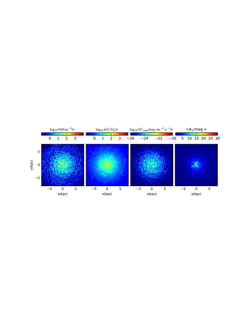
Figure 1: Left to right: distribution maps of the gas density, FUV flux, mechanical heating rate and the $A_{V}$ of the model disk galaxy. The galaxy is viewed face on where the averages (except $A_{\rm V}$) are computed by averaging along the line of sight.

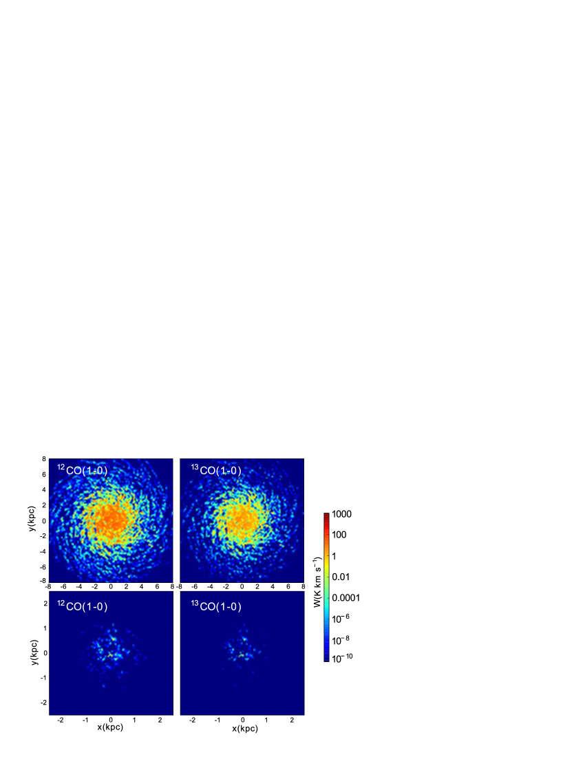
Figure 2: (Top row) CO($1-0$) and ¹³CO (1-0) fluxes of the disk galaxy. (Bottom row) CO(1-0) and ¹³CO (1-0) emission for the dwarf galaxy. The pixel size in these maps is 0.16 $\times$ 0.16 kpc.

We demonstrate the construction of the data cube, described in Section-2.4, by presenting the CO$(1-0)$ emission map of the disk galaxy in Figure-3. These maps provide insight on the velocity distribution of the gas along the line-of-sight. In the coordinate system we chose, negative velocities correspond to gas moving away from the observer, where the galaxy is viewed face-on in the sky. Thus, the velocities of the clouds are expected to be distributed around a zero mean. The width in the velocity distribution varies depending on the spatial location in the galaxy. For example, at the edge of the galaxy the gas is expected to be quiescent, with a narrow distribution in the line-of-sight velocities ($V_{\rm los}$). This is seen clearly in the channel maps $|V_{\rm los}|=20$ ${\rm km\leavevmode\nobreak\ s}^{-1}$ , where the CO$(1-0)$ emission is too weak outside the $R>3$ kpc region. In contrast the emission of these regions are relatively bright in the $|V_{\rm los}|=0$ ${\rm km\leavevmode\nobreak\ s}^{-1}$ map. In the inner regions, $R<1$ kpc, the CO$(1-0)$ emission is present even in the 40 ${\rm km\leavevmode\nobreak\ s}^{-1}$ channel, which is a sign of the wide dynamic range in the velocities of the gas at the central parts of the galaxy.

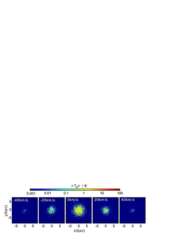
Figure 3: Channel maps of the CO($1-0$) emission of the disk galaxy. The width of each velocity channel is 20 ${\rm km\leavevmode\nobreak\ s}^{-1}$ , where the centroid of the velocity channel, is indicated at the top of each panel. Since the galaxy is projected face-on at the sky, most of the emission emanates from the channel [-10, 10] ${\rm km\leavevmode\nobreak\ s}^{-1}$ centered at $V_{\rm los}=0$ ${\rm km\leavevmode\nobreak\ s}^{-1}$ .

The relationship between excitation temperature, $T_{\rm ex}$ of the CO($1-0$) line, the distance of the molecular gas from the center of the galaxy ($R$) and mechanical feedback is illustrated in Figure-4; we plot the averages of $\Gamma_{\rm mech}$ $/n$, the mechanical heating rate per H nucleus, and the mean $T_{\rm ex}$ of the SPH particles in each pixel of the emission maps. $T_{\rm ex}$ for each SPH particle is a by product of the RADEX LVG computations (Schöier et al., 2005). We highlight the two obvious trends in the plots: (a) The mechanical heating per H nucleus increases as the gas is closer to the center, (b) The excitation temperature correlates positively with mechanical feedback and correlates negatively with distance from the center of the galaxy. It is also interesting to note that, on average, the SPH particles with the highest $\Gamma_{\rm mech}$ $/n$ have the highest excitation temperatures and are the closest to the center, see red points in the middle panel of Figure-4. On the other hand, gas situated at $R>3$ kpc has average excitation temperatures less than 10 K and approaches 2.73 K, the cosmic microwave background temperature we chose for the LVG modeling, at the outer edge of the galaxy. This decrease in the excitation temperature is not very surprising, since at the outer region CO is not collisionally excited due to collisions with H₂, which has a mean abundance 10 times lower than that of the central region. Collisional excitation depends strongly on the kinetic temperature of the gas. In Kazandjian et al. (2012), it was shown that small amounts of $\Gamma_{\rm mech}$  are required to double the kinetic temperature of the gas in the molecular zone, where most of the molecular emission originate. However, $\Gamma_{\rm mech}$  is at least 100 times weaker in the outer region compared to the central region, which renders mechanical feedback ineffective in collisionally exciting CO.

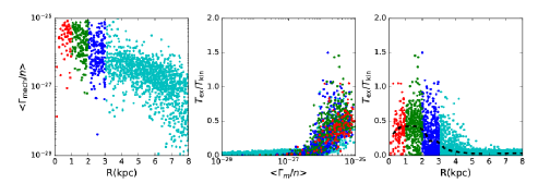
Figure 4: (Left) Mean mechanical heating per hydrogen (in erg s^-1) nucleus as a function of the distance from the center of the disk galaxy.(Center) The ratio of the mean excitation temperature of the CO(1-0) line to mean kinetic temperature as a function of mechanical heating rate per hydrogen nucleus. (Right) The ratio of the mean excitation temperature of the CO(1-0) line to mean kinetic temperature as a function of the distance from the center of the disk galaxy. The different colors correspond different galactocentric distance intervals. Red, green blue and cyan correspond to intervals [0, 1], [1,2] [2,3] and [3, 8] kpc respectively.

3.2 The X factor: correlation between CO emission and H₂ column density

Since H₂ can not been observed through its various transitions in cold molecular gas whose $T_{{\rm kin}}<100$ K, astronomers have been using the molecule CO as a proxy to derive the molecular mass in the ISM of galaxies. It has been argued that the relationship between CO(1-0) flux and $N(\rm H_{2})$ is more or less linear (Solomon et al., 1987; Bolatto et al., 2013, and references therein) with $X_{\rm CO}=N({\rm H}_{2})/W_{{\rm CO}(1-0)}$ nearly constant, where the proportionality factor $X_{\rm CO}$ is usually referred to as the $X$-factor. The observationally determined Milky Way $X_{\rm CO}$, $X_{\rm CO,MW}$, is given by $\sim 2\times 10^{20}$ cm^-2 (${\rm K\leavevmode\nobreak\ km\leavevmode\nobreak\ s}^{-1}$ )^-1 (Solomon et al., 1987). By using the emission map of CO(1-0) presented in Figure-2, and estimating the mean $N({\rm H}_{2})$ throughout the map from the PDR models, we test this relationship in Figure-5.

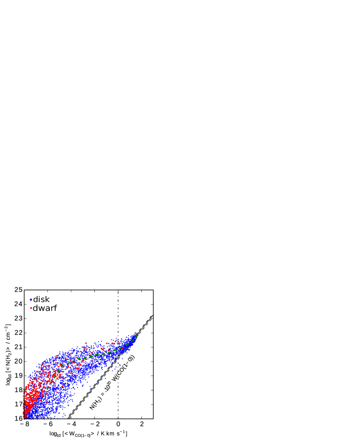
Figure 5: $N({\rm H}_{2})$ vs. CO(1-0) flux of the synthetic emission maps for the disk and dwarf galaxies. The blue and red points correspond to the pixels of the disk and dwarf galaxies respectively. The solid black line is the $W_{{\rm CO}(1-0)}=X_{\rm CO,MW}$ $N({\rm H}_{2})$ curve, with the observed $\pm 30\%$ uncertainty band (Bolatto et al., 2013) shown by the black dashed lines. This uncertainty could be up to a factor of two under a variety of conditions. $X_{\rm CO}$ for pixels with $W_{{\rm CO}(1-0)}<10$ ${\rm K\leavevmode\nobreak\ km\leavevmode\nobreak\ s}^{-1}$ diverges from that of the Milky way, where the mean $X_{\rm CO}$ for the pixels is plotted in green. We note that 99% of the luminosity of the disk galaxy emanates from pixels whose $W_{{\rm CO}(1-0)}>1$ ${\rm K\leavevmode\nobreak\ km\leavevmode\nobreak\ s}^{-1}$ indicated by the dot-dashed line.

It is clear that only for pixels with $W_{{\rm CO}(1-0)}>10$  ${\rm K\leavevmode\nobreak\ km\leavevmode\nobreak\ s}^{-1}$ $X_{\rm CO}$ approaches $X_{\rm CO,MW}$. These pixels are located within $R\lesssim 2$ kpc of the disk galaxy, and $R\lesssim 0.2$ kpc of the dwarf galaxy. Whenever $W_{{\rm CO}(1-0)}<10$  ${\rm K\leavevmode\nobreak\ km\leavevmode\nobreak\ s}^{-1}$ , $X_{\rm CO}$ increases rapidly reaching $\sim 1000X_{\rm CO,MW}$. Looking closely at pixels within $W_{{\rm CO}(1-0)}$ intervals of $[0.1,1]$, $[1,10]$ and $>10$ ${\rm K\leavevmode\nobreak\ km\leavevmode\nobreak\ s}^{-1}$ we see that the gas average densities in these pixels are $\sim 20,80$ and 300 cm^-3 respectively. This indicates that as the gas density becomes closer to the critical density, $n_{\rm crit}$, of the CO(1-0) transition, which is $\sim 2\times 10^{3}$cm^-3 , $X_{\rm CO}$ converges to that of the Milky Way. This is not surprising since as the density of gas increases, the mean $A_{V}$ of an SPH particle increases to more than 1 mag. In most cases, beyond $A_{V}>1$ mag, most of the H and C atoms are locked in H₂ and CO molecules respectively, where their abundances become constant. This leads to a steady dependence of the CO emission on $A_{V}$, and hence H₂. This is not the case for $A_{V}<1$ mag, where strong variations in the abundances of H₂ and CO result in strong variations in the column density of H₂ and the CO emission, leading to the spread in $X_{\rm CO}$ observed in Figure-5. A more precise description on this matter is presented by Bolatto et al. (2013).

Most of the gas of the dwarf galaxy lies in the $A_{V}<1$ mag range. Moreover, the low metallicity of dwarf galaxy results in a smaller abundance of CO in comparison to the disk galaxy, and thus a lower $W_{{\rm CO}(1-0)}$. This results in an $X_{\rm CO}$ which is 10 to 100 times higher than that of the Milky Way (Leroy et al., 2011). Our purpose of showing Figure-5 is to check the validity of our modeling of the emission. Maloney & Black (1988) provide a more rigorous explanation on the $W_{{\rm CO}(1-0)}$ and $N({\rm H}_{2})$ relationship.

3.3 Higher $J$-transitions

So far we have only mentioned the CO(1-0) transition. The critical density of this transition is $2\times 10^{3}$ cm^-3 . The maximum density of the gas in our simulations is $\sim 10^{4}$ cm^-3 . It is necessary to consider higher $J$ transitions in probing this denser gas. The critical density of the CO(4-3) transition is $\sim 10^{5}$ cm^-3 , which corresponds to densities 10 times higher than the maximum of our model galaxies. Despite this difference in densities the emission of this transition and the intermediate ones, $J=2-1$ and $J=3-2$, are bright enough to be observed due to collisional excitation mainly with H₂ . To have bright emission from these higher $J$ transitions, it also necessary for the gas to be warm enough, with $T_{\rm kin}\gtrsim 50$ K, so that these levels are collisionally populated. In Figure-6, we show the luminosities of the line emission up to $J=4-3$ of CO and ¹³CO , emanating from the disk and dwarf galaxies. In addition to that, we present the luminosity of the inner, $R<0.5$ kpc, region of the disk galaxy where $\Gamma_{\rm mech}$  is enhanced compared to the outer parts. This allows us to understand the trend in the line ratios and how they spatially vary and how mechanical feedback affects them (see next section). The ladders of both species are somewhat less steep for the central region, which can be seen when comparing the black and red curves of the disk galaxy in Figure-6. Hence, the line ratios for the high-$J$ transitions to the low-$J$ transitions are larger in the central region. This effect of $\Gamma_{\rm mech}$  was also discussed by Kazandjian et al (2015), who also showed that line ratios of high-$J$ to low-$J$ transitions are enhanced in regions where mechanical heating is high, which is also the case for the central parts of our disk galaxy. We will look at line ratios and how they vary spatially in Section-3.4.

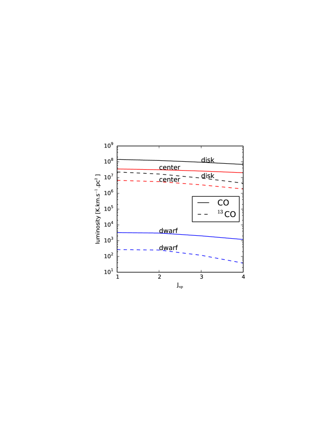
Figure 6: Total luminosity of CO and ¹³CO  transitions up to $J=4-3$ of the disk galaxy (black curves), the $R<2$ kpc region of the disk galaxy (red curves) and the dwarf galaxy (blue curves).

3.4 Diagnostics

In this section we use synthetic emission maps, for the $J>1-0$ transitions, constructed in a similar fashion as described in Section-3.1. These maps are used to compute line ratios among CO and ¹³CO   lines where we try to understand the possible ranges in diagnostic quantities. This can help us recover physical properties of a partially resolved galaxy.

In Figure-7, we show ratio maps for the various transitions of CO and ¹³CO . In these maps, line ratios generally exhibit uniform distributions in the regions where $R<2$ kpc. This uniform region shrinks down to 1 kpc as the emission from transition in the denominator becomes brighter. This is clearly visible when looking at the corresponding ¹³CO /CO line rations in the panels along the diagonal of Figure-7. This is also true for the CO/CO transitions shown in the upper right panels of the same figure. Exciting the $J>$ $1-0$ transitions requires enhanced temperatures, where $\Gamma_{\rm mech}$  and H₂ densities higher than $10^{3}$ cm^-3 plays an important role. Such conditions are typical to the central 2 kpc region that result in bright emission of $J>1-0$ transitions and lead to forming the compact peaks within that region that we mentioned. The peak value of the line ratios of CO/CO transitions at the center is around unity, compared to 0.1 - 0.3 for ratios involving transitions of ¹³CO /CO. Since $J>1-0$ transitions are weakly excited outside the central region, the line ratios decrease, e.g., by factors of 3 to 10 towards the outer edge of the galaxy for CO(2-1)/CO(1-0) and CO(4-3)/CO(1-0), respectively. Another consequence of the weak collisional excitation of CO and ¹³CO   is noticed by looking again at the ¹³CO /CO transitions along the diagonal panels of Fig-7, where the small scale structure of cloud “clumping”, outside the central region becomes evident by comparing the ¹³CO (1-0)/CO(1-0) to ¹³CO (4-3)/CO(4-3). This dense gas is compact and occupies a much smaller volume and mass, approximately 10% by mass.

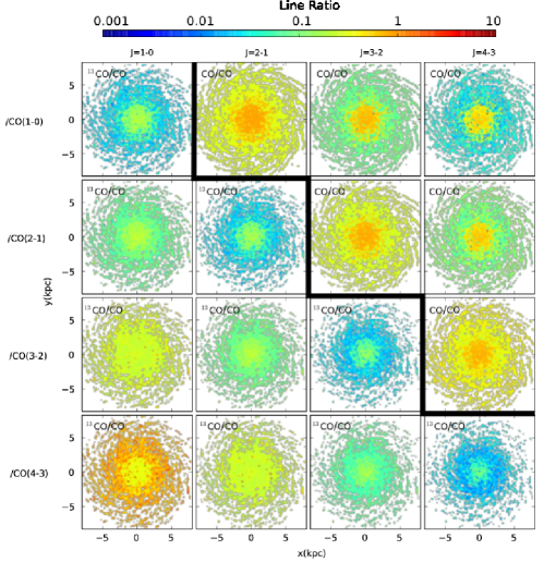
Figure 7: Line ratio maps for various transitions of CO and ¹³CO   for the disk galaxy. The transition of the line in the numerator is specified at the top of each column, whereas that of the denominator is specified at the left of each row. For example, the panel in the third row of the second column corresponds to the line ratio map of ¹³CO (2-1)/CO(3-2); the species involved in the line ratio are specified at the top left corner of each panel. Ratios larger than unity are typical to the central regions $R<2$ kpc. Line ratio maps between CO transitions are to the right of the zig-zagged line, whereas the remaining maps are for line ratios between ¹³CO   and CO. Ratios involving $J\geq 3-2$ transitions trace the small scale structure of the molecular gas for $R>2$ kpc.

Similar line ratio maps can be constructed for the dwarf galaxy, which are presented in Figure-A3 of the Appendix. These maps can be used to constrain the important physical parameters of the gas of both model galaxies, as we will demonstrate in the next section.

4 Application: modeling extra-galactic sources using PDRs and mechanical feedback

Now that we have established the spatial variation of diagnostic line ratios in the synthetic maps, we can use them to recover the physical parameters of the molecular gas that is emitting in CO and ¹³CO .

The synthetic maps that we have constructed assume a high spatial resolution of 100 $\times$ 100 pixels, where the size of our model disk galaxy is $\sim 16$ kpc. If we assume that the galaxy is in the local universe at a fiducial distance of 3 Mpc (the same distance chosen by Pérez-Beaupuits et al. (2011)), which is also the same distance of the well known galaxy NGC 253, then it is necessary to have an angular resolution of 1” to obtain such a resolution. This can be easily achieved with ALMA where it can easily achieve a resolution of 0.1” at all the frequency bands it operates in. A grid of size 21 $\times$ 21 is used to allow for a $\sim 0.8$kpc resolution per pixel, which is a typical resolution that can be achieved with single-dish studies of nearby galaxies such as the HERACLES/IRAM-30m survey (Leroy et al., 2009).

In the top panel of Figure-8, we show the normalized $W_{{\rm CO}(1-0)}$ map, normalized with respect to the peak flux, with an overlaid mesh of the resolution mentioned before. We re-compute the emission maps for all the CO and the ¹³CO  lines using the 21 $\times$ 21 pixel grid. Each pixel in the mesh contains on average a few thousand SPH particles. In what follows we treat these synthetic emission maps as input and try to find the best fitting mPDR models by following a minimization procedure applied to a certain pixel. Using the emission computed from the PDR models, we estimate the parameters $n,G,\Gamma_{\rm mech}$ and $A_{V}$ that best fit the emission of that pixel. Since we consider transitions up to $J=4-3$ for CO and ¹³CO , we have a total of 8 transitions, hence $8-4=4$ degrees of freedom in our fits. The purpose of favoring one PDR component in the fitting procedure is not to reduce the degrees of freedom, since for every added PDR component we lose five degrees of freedom, which could result in fits that are less significant.

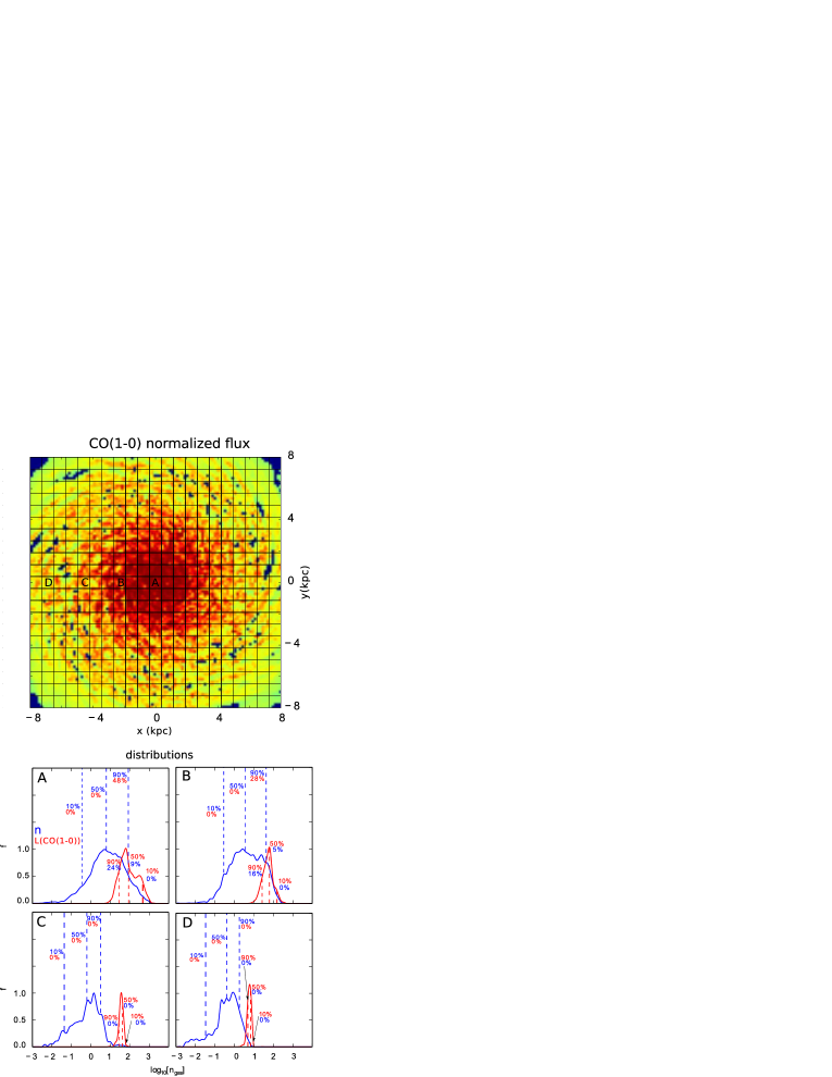
Figure 8: Distributions of gas density and $W({\rm CO}(1-0))$ as a function of distance from the center of the disk galaxy. The normalized $W_{{\rm CO}(1-0)}$ map, with the overlaid grid which has a resolution of $21\times 21$ pixels is show in the Upper panel. The labels A, B, C, D correspond to the pixels at distances of 0, 2, 4, and 7 kpc from the center of the galaxy. In the bottom panels we plot, in blue, the gas density distribution function, $f(n)$, of the SPH particles in these pixels. The fractional contribution of the SPH particles to the CO(1-0) luminosity of the pixel as a function of gas density, $f(L_{{\rm CO}(1-0)})(n)$, is plotted in red. Both curves are scaled to their maximum value so that we can compare the ranges where they overlap. The cumulative distribution function is defined as ${\rm CDF}(n)=\int_{10^{-3}}^{n}f(n)dn$. The blue dashed lines indicate the gas densities where the ${\rm CDF}=10,50,90$% respectively. Below these percentages, in red, are the fractional contribution of these SPH particles to the luminosity of the pixel. This contribution is defined as ${\rm LCDF}(n)=\int_{10^{-3}}^{n}f(L_{{\rm CO}(1-0)})(n)dn$. The red dashed lines represent the ${\rm LCDF}=\int_{n}^{10^{4}}f(L_{{\rm CO}(1-0)})(n)dn$ along with the analogous CDF integrated from $n=10^{4}$ cm^-3 . The corresponding distribution plots as a function of $G_{0}$, $\Gamma_{\rm mech}$  and $A_{V}$ are shown in Figure-A2 in the appendix.

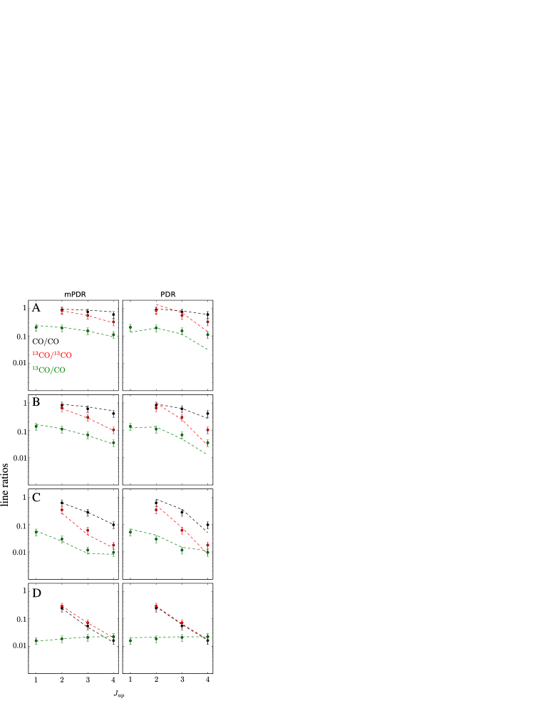
Figure 9: Constraining the parameters for a resolved galaxy. The black dots correspond to the line ratios of CO($J\geq 2-1$) with CO(1-0) for a pixel in the emission map. The red dots correspond to the line ratios of ¹³CO ($J\geq 2-1$) with ¹³CO (1-0) for the same pixel. The green dots correspond to the line ratios of the same transitions of ¹³CO   and CO for a pixel. The dashed line are the line ratios of these transitions of the best fit PDR model. The PDR models in the left column labeled “mPDR” consider a range of possible $\Gamma_{\rm mech}$ in the heating budget while fitting these line ratios (the dots), while the plots labeled “PDR” do not take $\Gamma_{\rm mech}$  into account. The labels A, B, C, and D correspond to the pixels indicated in the top panel of Figure-8. The parameters of the best fit PDR models for each pixel are listed in Table-2.

The statistic we minimize in the fitting procedure is :

$$\chi^{2}=\sum_{j}\sum_{i}\left[\frac{(r^{i}_{o}-r^{j}_{m})}{\sigma^{i}_{o}}\right]^{2}$$ (2)

(Press et al., 2002), where $r_{o}$ and $\sigma_{o}$ are the observed values and assumed error bars of the line ratios of the pixel in the synthetic map. $r_{m}$ is the line ratio for the single PDR model whose parameter set we vary to minimize $\chi^{2}$. The index $i$ corresponds to the different combinations of line ratios. The line ratios we try to match are the CO and ¹³CO   ladders normalized to their $J=1-0$ transition, in addition to the ratios of ¹³CO   to the CO ladder. These add up to 10 different line ratios which are not independent, and the number of degrees of freedom remains 4 for the mechanically heated model (mPDR), and 3 for the PDR which does not consider mechanical heating.

In Figure-9, we show the fitted line ratios of the pixels labeled (A, B, C, D) in Figure-8. The first row, labeled A, corresponds to the central pixel in the map. For this pixel, 90% of the emission emanates from gas whose density is higher than 10 cm^-3 , constituting 24% of the mass in that pixel. The normalized cumulative distribution functions for the gas density (blue curves) and CO(1-0) luminosity (red curves) are shown in the bottom panels of Figure-8. The blue dashed lines indicates the density where 10, 50 and 90% of the SPH particles have a density up to that value. The numbers in red below these percentages indicate the contribution of these particles to the total luminosity of that pixel. For instance, in pixel A 10% of the particles have a density less than $\sim 0.03$ cm^-3 and these particles contribute 0% to the luminosity of that pixel; at the other end, 90% of the particles have a density less than $\sim 100$ cm^-3 and these particle contribute 48% to the luminosity of that pixel. In a similar fashion, the red dashed lines show the cumulative distribution function of the CO(1-0) luminosity of the SPH particles, but this time integrated from the other end of the $n$ axis. For example, 50% of the luminosity results from particles whose density is larger than 100 cm^-3 . These particles constitute 9% of the gas mass in that pixel. The fits for PDR models that do not consider mechanical heating are shown in Figure-9. We see that these models fit ratios involving $J>3-2$ transitions poorly compared to the mPDR fits, especially for the pixel A and B which are closer to the center of the galaxy compared to pixels C and D. In the remaining rows (B,C,D) of Figure-9, we show fits for pixels of increasing distances from the center of the galaxy. We see that as we move away further from the center, the CO to ¹³CO  ratios become flat in general, close to the elemental abundance ratio of ¹³C/C which is 1/40 (see the green curve in the bottom row). This is essential, because the lines of both species are optically thin at the outer edge of the galaxy, hence the emission is linearly proportional to the column density, which is related to the mean abundance in the molecular zone. Another observation is that the distribution of the luminosity in a pixel becomes narrow at the edge of the galaxy. This is due to the low gas density and temperature in this region, where there are less SPH particles whose density is close to the critical density of the CO(1-0) line. We also see that $\Gamma_{\rm mech}$  plays a minor role, where both fits for a PDR with and without $\Gamma_{\rm mech}$  are equally significant. The parameters of the fits for the four representative pixels are listed in Table-2.

		$\log_{10}\left[\frac{n}{{\rm cm}^{-3}}\right]$	$\log_{10}\left[\frac{G}{G_{0}}\right]$	$\log_{10}\left[\frac{\Gamma_{\rm mech}}{{\rm erg\leavevmode\nobreak\ cm}^{-3}{\rm\leavevmode\nobreak\ s}^{-1}}\right]$	$\frac{A_{V}}{{\rm mag}}$	$\chi^{2}_{\rm red}$
disk
galaxy
A	mPDR	$1.8\pm 0.1$	$1.4\pm 1.0$	$-23.0\pm 0.1$	$22\pm 2$	$0.5\pm 0.1$
0.5 kpc	PDR	$3.5\pm 0.1$	$4.7\pm 0.3$	–	$7.6\pm 0.4$	$3.7\pm 0.1$
	Actual	$1.63\pm 0.1$	$1.71\pm 0.1$	$-23.1\pm 0.1$	$9.8\pm 0.7$	–
B	mPDR	$1.2\pm 0.3$	$0.6\pm 0.9$	$-23.5\pm 0.3$	$20.9\pm 3.1$	$0.7\pm 0.2$
2 kpc	PDR	$3.5\pm 0.1$	$2.8\pm 0.4$	–	$5.1\pm 0.6$	$3.6\pm 0.2$
	Actual	$1.16\pm 0.2$	$1.22\pm 0.1$	$-23.8\pm 0.2$	$4.7\pm 0.7$	–
C	mPDR	$1.5\pm 0.3$	$3.7\pm 1.1$	$-23.8\pm 0.3$	$10.1\pm 2.4$	$1.1\pm 0.2$
4 kpc	PDR	$2.7\pm 0.3$	$4.2\pm 0.7$	–	$6.6\pm 1.2$	$3.0\pm 0.8$
	Actual	$0.41\pm 0.1$	$0.53\pm 0.1$	$-24.9\pm 0.2$	$1.4\pm 0.1$	–
D	mPDR	$0.7\pm 0.5$	$1.6\pm 1.3$	$-26.5\pm 1.2$	$3.6\pm 1.7$	$0.3\pm 0.3$
7 kpc	PDR	$0.7\pm 0.6$	$3.3\pm 0.9$	–	$4.9\pm 1.5$	$0.6\pm 0.4$
	Actual	$-0.23\pm 0.1$	$-0.18\pm 0.1$	$-26.6\pm 0.2$	$0.4\pm 0.1$	–
dwarf
galaxy
	mPDR	$2.5\pm 0.3$	$3.4\pm 0.8$	$-23.4\pm 0.3$	$4.2\pm 0.6$	$0.6\pm 0.4$
0.5 kpc	PDR	$2.5\pm 0.3$	$4.7\pm 0.4$	–	$5.4\pm 0.4$	$0.5\pm 0.3$
	Actual	$1.1\pm 0.1$	$1.33\pm 0.1$	$-24.9\pm 0.2$	$0.8\pm 0.1$	–

Table 2: A comparison between the parameters fit using line ratios for the disk and dwarf galaxy. The listed numbers are the averages of the fit parameters for pixels at a specific distance from the center, these distances are listed on the left of the Table. For the dwarf galaxy we only show the fit parameters for the central 0.5 kpc. For each pixel, we present the fit parameter (first row) for a mechanically heated PDR (mPDR), a pure PDR which does not consider mechanical feedback into its heating budget (second row), and the actual mean and standard deviation for these quantities for the SPH particles within the pixel of the luminosity map. In the last column the statistic we minimize per degree of freedom, $\chi^{2}_{\rm red}$ is listed to compare the quality of the fits of the mPDR and the pure PDR models.

This fitting procedure can also be applied to the dwarf galaxy. The main difference in modeling the gas as a PDR in the disk and dwarf galaxy is that the mechanical heating in the dwarf is lower compared to the disk, thus it does not make a significant difference in the fits. In Figure-A3, the line ratio maps show small spatial variation, thus it is not surprising in having small standard deviations in the fit parameters, in Table-2 of the dwarf galaxy compared to the disk galaxy. We note that the for regions at the outskirts of the disk galaxy such as pixel C and D, we see significant deviations of the recovered values of $n$, $G$, and $A_{\rm V}$ from the mPDR and PDR models. For the mPDR models $\Gamma_{\rm mech}$ the deviation could be due to degeneracies imposed by the strong dependence of the emission on $\Gamma_{\rm mech}$ in this relatively “low” density region compared to the central region where $\Gamma_{\rm mech}$   is the dominant heating mechanism. As for the deviation of the best fit PDR model for these pixels, they could be linked to the fact that the quality of the fit is poor as indicated by the large $\chi^{2}$ values. An advantage of using PDR models is that they do a better job at recovering the actual value of $A_{\rm V}$ for pixels such as A and B ($R<2$ kpc), but these fits are statistical less significant than the mPDR fits and they do not provide information about the mechanical heating rate.

5 Conclusion and discussion

In this paper, we have presented a method to model molecular species emission such as CO and ¹³CO  for any simulation which includes gas and provides a local mechanical heating rate and FUV-flux. The method uses this local information to model the spatial dependence of the chemical structure of PDR regions assumed to be present in the sub-structure of the gas in the galaxy models. These are then used to derive brightness maps assuming the LVG approximation. The method for the determination of the emission maps together with the ISM model of the hydrodynamic galaxy models constitute a complete, self-consistent model for the molecular emission from a star forming galaxies’ ISM. We compute the emission of CO and ¹³CO   in rotational transitions up to $J=4-3$ for a model disk-like and a dwarf galaxy. From the emission maps line ratios were computed in order to constrain the physical parameters of the molecular gas using one component PDR models.

We conclude the following:

1. Excitation temperature correlates positively with mechanical feedback in equilibrium galaxies. This in turn increases for gas which is closer to the center of the galaxy. The analysis presented in this paper allows estimates of mechanical feedback in galaxies which have high excitation temperatures in the center such as those observed by, e.g., Mühle et al. (2007) and Israel (2009).

2. Fitting line ratios of CO and ¹³CO   using a single mechanically heated PDR component is sufficient to constrain the local $\Gamma_{\rm mech}$  throughout the galaxy within an order of magnitude, given the limitations of our modeling of the emission. The density of the gas emitting in CO and ¹³CO   is better constrained to within half dex. This approach is not suitable in constraining the gas parameters of the dwarf galaxy, although the statistical quality of the fits is on average better than that of the disk galaxy.

3. Our approach fails in constraining the local FUV-flux. It is under-estimated by two orders of magnitude in mechanically heated PDR fits, and over-estimated by more than that in PDRs, which do not account for mechanical feedback. This discrepancy is due considering one PDR component, where $J<3-2$ CO lines are optically thick and trace very shielded gas. This discrepancy can also be explained by looking at the right column of Figure-A2, where most of the emission results from SPH particles, which constitute a small fraction, and the rest of the gas is not captured by the PDR modeling.

The main features of our PDR modeling with mechanical feedback is the higher number of degrees of freedom it allows compared to LVG models and multi-component PDR modeling. We fit 10 line ratios while varying four parameters in the case where $\Gamma_{\rm mech}$  was considered, and 3 parameters when $\Gamma_{\rm mech}$  was not. We note that the actual number of independent measurements of line emission of CO and ¹³CO  up to $J=4-3$ is 8. In LVG modeling the number of free parameters is at least 5, since in fitting the line ratios we need to vary $T$, $n({\rm H}_{2}$), $N$(CO), N(¹³CO ) and the velocity gradient. On the other hand, PDR models assume elemental abundances and reaction rates. Moreover, the uncertainties in the PDR modeling could be much larger and depend on the micro-physics used in the PDR modeling (Vasyunin et al., 2004; Röllig et al., 2007). Thus, LVG models have more free parameters compared to single PDR models used in our method. On the other hand, considering two PDR components increases the number of free parameters to 9. This renders the fitting problem over-determined with more free parameters than independent measurements. Although LVG models are simple to run compared to PDR models, they do not provide information about the underlying physical phenomena exciting the line emission, which renders them useless for constraining $\Gamma_{\rm mech}$ . Although a two component PDR model produces better “Xi-by-eye” fits, these fits are statistically less significant than a single PDR model, but physically relevant. The main disadvantage of PDR modeling is the amount of bookkeeping required to run these models and they are computationally more demanding than LVG modeling, which is why we resorted to using interpolation tables.

5.1 Improvements and prospects

Our models have two main limitations: 1) we make implicit assumptions on the small scale structure of the galactic ISM and 2) we assume chemical equilibrium. The first limitation can be improved by performing higher spatial resolution simulations, which would result in gas that is better resolved and is denser than the current maximum of $10^{4}$ cm^-3 in the disk galaxy. Gas densities $>10^{6}$ cm^-3 allows us to consider transitions up to $J=15-14$ which are more sensitive to $\Gamma_{\rm mech}$  compared to the $J=1-0$. Galaxy scale simulations, which reach densities higher than $10^{4}$ cm^-3  have been performed by Narayanan & Hopkins (2013) and required about $3\times 10^{7}$ particles, and our method could be easily scaled to post-process such simulations. In a follow up paper (Kazandjian et al., 2016) we re-sampled the gas density distribution of the disk simulation used in this paper in-order to probe the effect of $n\gtrsim 10^{4}$ cm^-3 gas on the emission of $4-3<J\leq 15-14$ transitions of CO and ¹³CO , in addition to $J\leq 7-6$ transitions of HCN, HNC, and ${\rm HCO}^{+}$ and their associated diagnostic line ratios on galactic scales.

Having more data to fit helps in finding better diagnostics of $\Gamma_{\rm mech}$   and narrower constraints for it. Another advantage in having emission maps for these high $J$ transitions is having a higher number of degrees of freedom in fitting for the emission line ratios. This renders the best fit PDR models statistically more significant. Moreover, it would be natural to consider multi-components PDR models in these fits, a dense-component fitting the $J>4-3$ transitions and low-density component fitting the lower ones. These components are not independent, low-$J$ emission is also produced by the high density PDR components. The high density component PDR would generally have a filling factor 10 to 100 times lower than the low density component, thus the high density model contributes mainly to the high-$J$ transitions, whereas the low density models contributes mainly to the low-$J$ emission and less to the high-$J$ emission.

In producing the synthetic line emission maps, we have used the LVG emission from SPH particles, which assume PDR models as the governing sub-grid physics. The main assumption in computing the emission using LVG models was the fixed value of the micro-turbulence line-width $v_{\rm turb}=1$ km/s for all the SPH particles. The peak of the distribution of $v_{\rm turb}$ of the SPH particles is located at $\sim 3$ km/s. The optical depth in the lines are thus in reality smaller than what we used in the calculations for the paper. When the lines become optically thick it effectively reduces the critical density of those transitions, and allows the excitation to higher energy states. The lines become more easily optically thick, for normal cloud sizes ($A_{\rm V}=5-10$) at $v_{\rm turb}=1$ km/s, which causes the peak of the CO ladder to be at a higher rotational transition. In order to quantify the shift of the peak of the CO ladder, we calculated a grid with different turbulent velocities, $v_{\rm turb}=1.0,2.7,5.0$, and 10.0 km/s, representative of the turbulent velocities in the SPH simulation, and used that grid to produce the resulting CO ladder. We found that the peak of the CO ladder is located at CO(4-3) transition, when computed from the distribution of $v_{turb}$, while the peak is located at CO(6-5) for the calculations where only $v_{\rm turb}=1.0$ km/s was used. Although this causes a significant quantitative change in the emission, it does not affect the general conclusions of the paper. A possible consequence of considering $v_{\rm turb}$ to be constant is the fact that the ¹³CO /CO line rations increase towards the center of our model galaxies and are close to the elemental abundance ratio of ${}^{12}{\rm C}/^{13}{\rm C}$ $\sim 40$ in contrast to observations where this ratio ranges between 8 and 15 (e.g. Buchbender et al., 2013, and references therein). The emission of CO are enhanced towards the center due to the increasing temperature of the gas. Accounting for $v_{\rm turb}$ would most likely enhance the relative emission of CO compared to ¹³CO  where the computed line-ratios of the model galaxies would be in-line with the observed trends and could also reduce ${}^{12}{\rm C}(1-0)/^{13}{\rm C}(1-0)$ to the observed range of, which is currently a limitation to our proposed modelling approach.

An accurate treatment of the radiative transfer entails constructing the synthetic maps by solving the 3D radiative transfer of the line emission using tools such as LIME (Brinch & Hogerheijde, 2010). This would eliminate any possible bias in the fits. Currently, we construct the emission maps by considering the mean flux of the emission of SPH particles modeled as PDR within a pixel. This results in a distribution of the emission as a function of gas density as seen in Figure-8 and Figure-A2. When fitting the line ratios, we recover the mean physical parameters of the molecular gas in that pixel associated with these emission. Using tools such as LIME, the micro-turbulence line width would be treated in a more realistic way by using the actual local velocity dispersions in the small scale turbulent structure of the gas, as opposed to adopting a fiducial 1 ${\rm km\leavevmode\nobreak\ s}^{-1}$ as we have done throughout the paper. A major limitation of our sub-grid modelling is the assumption that the FUV flux at the surface of the PDR corresponds to that of the environment of the SPH particle. The FUV flux and the FUV-driven heating is strongly attenuated by the intervening dusty CNM, and the H₂ clouds embedded in it. This is in contrast to turbulent and cosmic ray heating that operate over large gas volumes. An accurate treatment of the FUV radiative transfer could influence the modeled abundances of the molecular species and consequently the computed line emission fluxes. that are used as diagnostics.

Not all H₂ gas is traced by CO, since the H/H₂ transition zone occurs around A${}_{V}=0.1$ mag whereas the C/CO transition occurs around A${}_{V}=1$ mag. When looking at Figure-8 and Figure-A2, we see that most of the CO emission emanates from a fraction of the gas. The remaining “major” part of the gas can contain molecular H₂, which is not traced by CO, but by other species such as C or C⁺, that do have high enough abundances to have bright emission (Madden et al., 1997; Papadopoulos et al., 2002; Wolfire et al., 2010; Pineda et al., 2014; Israel et al., 2015).

Finally, we note that we have ignored any “filling factor” effects in constructing the synthetic maps and the fitting procedure. This is not relevant to our method since in considering line ratios, and filling factors cancel out in single PDR modeling of line ratios. However, it is important and should be taken into account, when considering multi-component PDR modeling and when fitting the absolute luminosities.

Appendix-A

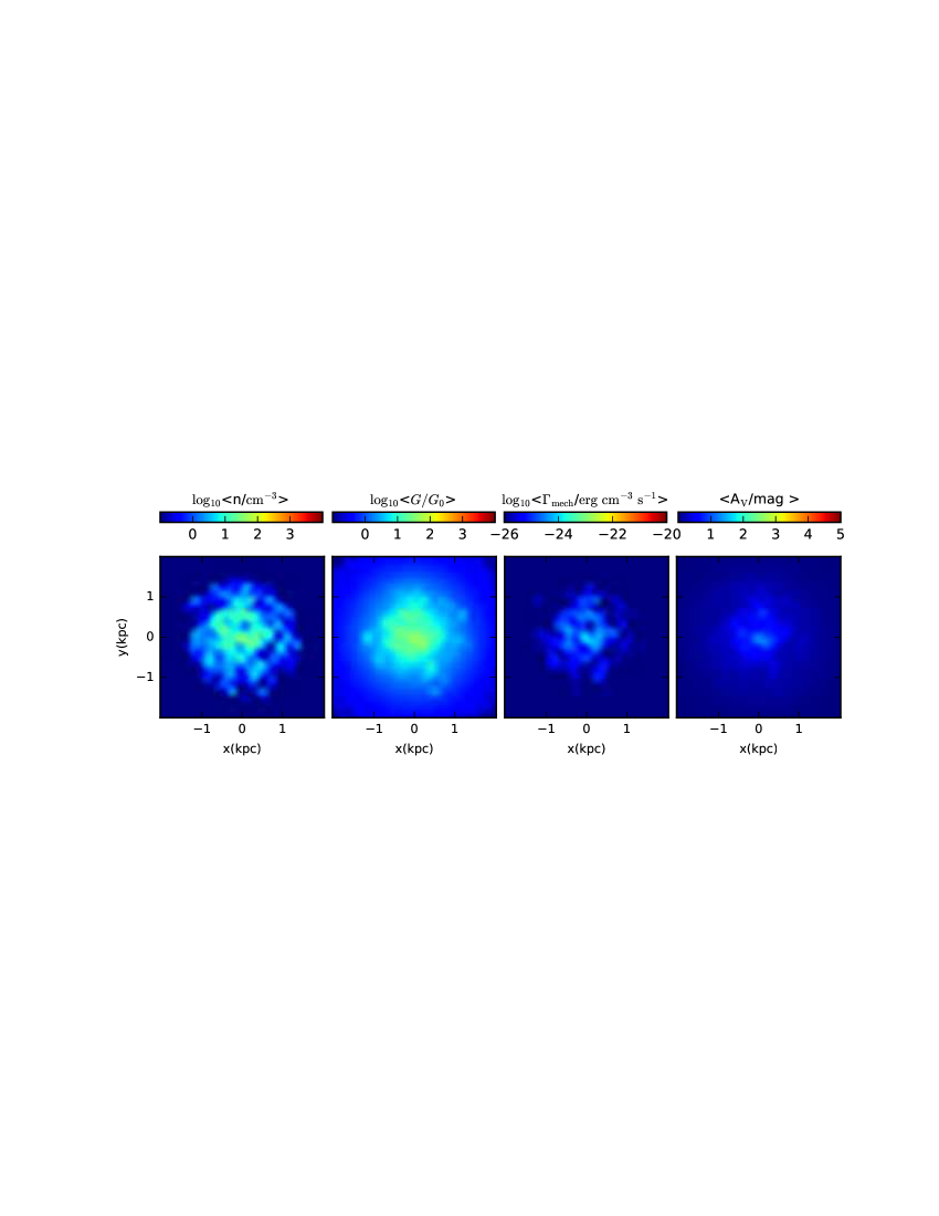
Figure A1: Left to right: distribution maps of the gas density, FUV flux, mechanical heating rate and the $A_{V}$ of the model dwarf galaxy.

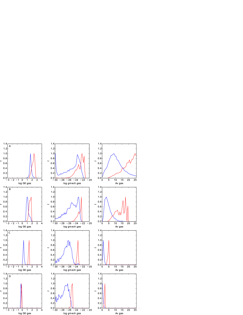
Figure A2: Distribution functions as a function of $G_{0}$, $\Gamma_{\rm mech}$  and $A_{V}$ for the representative pixels labeled A, B, C and D of Figure-8. The blue curves represent the distributions as a function of $G_{0}$ (first column), $\Gamma_{\rm mech}$  (second column) and $A_{V}$ (third column). The red curves represent the fractional contribution of these distributions to the luminosity of their corresponding pixels. Both curves are normalized to their peak so that we can visually compare the subset of these distributions which contribute to the luminosity.

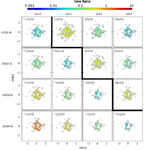
Figure A3: Line ratio maps for various transitions of CO and ¹³CO   for the dwarf galaxy. The line ratios are generally spatially uniform and show slight variation, unlike the disk galaxy. These maps are also patchy, especially for line ratios involving $J=3-2$ and $J=4-3$ transitions. This is due to the low number of SPH particles with densities close to $10^{4}$ cm^-3 which are a pre-requisites for these transitions. See caption of Figure-7 for more details on interpreting the maps.