Modelling Void Abundance in Modified Gravity

Abstract

We use a spherical model and an extended excursion set formalism with drifting diffusive barriers to predict the abundance of cosmic voids in the context of general relativity as well as $f(R)$ and symmetron models of modified gravity. We detect spherical voids from a suite of N-body simulations of these gravity theories and compare the measured void abundance to theory predictions. We find that our model correctly describes the abundance of both dark matter and galaxy voids, providing a better fit than previous proposals in the literature based on static barriers. We use the simulation abundance results to fit for the abundance model free parameters as a function of modified gravity parameters, and show that counts of dark matter voids can provide interesting constraints on modified gravity. For galaxy voids, more closely related to optical observations, we find that constraining modified gravity from void abundance alone may be significantly more challenging. In the context of current and upcoming galaxy surveys, the combination of void and halo statistics including their abundances, profiles and correlations should be effective in distinguishing modified gravity models that display different screening mechanisms.

I Introduction

The large scale structure of the Universe offers a promising means of probing alternative gravity theories Brax and Davis (2015); de Martino et al. (2015). Many models of modified gravity can be parameterized by a scalar degree of freedom that propagates an extra force on cosmologically relevant scales. Viable gravity theories must produce a background expansion that is close to that of a Lambda Cold Dark Matter ($\Lambda$CDM) model in order to satisfy current geometry and clustering constraints, and reduce to general relativity (GR) locally in order to satisfy solar system tests. The first feature may be imposed by construction or restriction of the parameter space whereas the latter feature relies on a nonlinear screening mechanism operating e.g. on regions of large density or deep potentials Brax (2012). Examples include $f(R)$ models with the chameleon mechanism Khoury and Weltman (2004a, b); Mota and Shaw (2007); Gannouji et al. (2010); Gubser and Khoury (2004); Navarro and Van Acoleyen (2007), braneworld models which display the Vainshtein mechanism Vainshtein (1972); Babichev and Deffayet (2013); Falck et al. (2014), and the symmetron model with a symmetry breaking of the scalar potential Hinterbichler and Khoury (2010); Hinterbichler et al. (2011); Hammami and Mota (2015); Davis et al. (2012). Most viable models of cosmic acceleration via modified gravity are nearly indistinguishable at the background level and may be quite degenerate, even when considering linear perturbation effects. However, different screening mechanisms operating on nonlinear scales are quite unique features of each model. It is therefore highly desirable to explore observational consequences that help expose these differences, despite the fact that nonlinear physics and baryonic effects must also be known to similar accuracy at these scales.

Investigating the nonlinear regime of modified gravity models requires N-body simulations Oyaizu (2008); Oyaizu et al. (2008); Schmidt et al. (2009); Schmidt (2009a, b); Clifton et al. (2005); Khoury and Wyman (2009); Li and Zhao (2009); Schmidt et al. (2010); Ferraro et al. (2011); Zhao et al. (2011); Li and Barrow (2011); Li et al. (2013); Wyman et al. (2013); Arnold et al. (2014); Brax et al. (2013); Candlish et al. (2015); Hagala et al. (2016); Achitouv et al. (2015); Hammami and Mota (2015); Winther et al. (2015); Barreira et al. (2016), in which one must solve nonlinear equations for the extra scalar field in order to properly account for screening mechanisms. From simulations one may extract the matter power spectrum on linear and non-linear scales Oyaizu et al. (2008); Schmidt (2009a, b); Khoury and Wyman (2009); Li and Hu (2011); Wyman et al. (2013); Taruya et al. (2014) as well as properties of dark matter halos, such as their abundance Schmidt et al. (2009); Schmidt (2009a); Bourliot et al. (2007); Schmidt (2009b); Li and Hu (2011); Zhao et al. (2011); Lombriser et al. (2013); Wyman et al. (2013), bias Schmidt et al. (2009, 2010); Zhao et al. (2011); Wyman et al. (2013) and profiles Schmidt et al. (2009); Schmidt (2009a); Zhao et al. (2011); Lombriser et al. (2012).

From the theoretical perspective, estimating e.g. the power spectrum in the nonlinear regime is non-trivial even for GR, and more so for modified gravity Koyama et al. (2009); Taruya et al. (2014), as the screening mechanisms must be properly accounted for in the evolution equations Brax and Valageas (2012). The halo model Cooray and Sheth (2002) provides an alternative to study these nonlinearities Schmidt et al. (2009, 2010), but it has its limitations even in standard GR. Moreover it requires accurate knowledge of various halo properties, including abundance, bias and profiles.

In GR the halo mass function may be estimated from the linear power spectrum and spherical collapse within the Press-Schechter Press and Schechter (1974) formalism and its extensions Sheth et al. (2001); Bond et al. (1991) or from empirical fits to simulations for higher precision Tinker et al. (2008); Jenkins et al. (2001). However for modified gravity screening mechanisms operate effectively within the most massive halos, and must be properly accounted for Li and Hu (2011). In addition, massive clusters have observational complications such as the determination of their mass-observable relation Lima and Hu (2005), which must be known to good accuracy in order for us to use cluster abundance for cosmological purposes. These relations may also change in modified gravity Arnold et al. (2014).

Cosmological voids, i.e. regions of low density and shallow potentials, offer yet another interesting observable to investigate modified gravity models Clampitt et al. (2013). Screening mechanisms operate weakly within voids, making them potentially more sensitive to modified gravity effects Pisani et al. (2015). One of the main issues for using voids is their very definition, which is not unique both theoretically and observationally. Compared to halos, the properties of voids have not been discussed in as much detail, although there have been a number of recent developments on the theory, simulations and observations of voids Sánchez et al. (2016); Pisani et al. (2015); Massara et al. (2015); Cai et al. (2016); Wojtak et al. (2016); Pollina et al. (2016); Nadathur and Hotchkiss (2015a, b); Nadathur et al. (2014).

Despite ambiguities in their exact definition, it has been observed in simulations that voids are quite spherical Sheth and van de Weygaert (2004), and therefore it is expected that the spherical expansion model for their abundance must work well (differently from halos, for which spherical collapse alone is not a very good approximation Corasaniti and Achitouv (2011a)). In this work, we use N-body simulations of $\Lambda$CDM as well as $f(R)$ and symmetron models of modified gravity in order to identify cosmic voids and study their abundance distribution. In order to interprete the simulation results, we use a spherical model and an extended excursion set formalism with underdense initial conditions to construct the void distribution function. Our extended model includes two drifting diffusive barriers in a similar fashion to the work from Maggiore and Riotto (2010a, b) to describe halo abundance. As a result, our model accounts for the void-in-cloud effect and generalizes models with static barriers Jennings et al. (2013).

We start in § II describing the parametrization of perturbations in $f(R)$ and symmetron gravity as well as the spherical model equations. In § III we use the excursion set formalism to model void abundance and in § IV we describe the procedure for void identification from simulations. Importantly, we define spherical voids in simulations with a criterium that is self-consistent with our predictions. In § V we present our main results, using simulations to fit for the model free parameters and studying constraints on modified gravity from ideal dark matter voids. We also study the possibility of using our model to describe galaxy voids. Finally, in § VI we discuss our results and conclude.

II Perturbations

The spherical evolution model is usually the first step to investigate the abundance of virialized objects tracing the Universe structure, such as halos, and likewise it is a promising tool for voids. It also offers a starting point to study the collapse of non-spherical structures Achitouv and Corasaniti (2012); Corasaniti and Achitouv (2011a) and the parameters required to quantify the abundance of these objects within extended models Zentner (2007).

The large scale structure of the Universe is well characterized by the evolution of dark matter, which interacts only gravitationally and can be approximated by a pressureless perfect fluid. The line element for a perturbed Friedmann-Lemaître-Robertson-Walker (FLRW) metric in the Newtonian gauge is given by

$$ds^{2}=-a^{2}(1+2\Psi)d\tau^{2}+a^{2}(1-2\Phi)dl^{2}\,,$$ (1)

where $a$ is the scale factor, $\tau$ is the conformal time related to the physical time $t$ by $ad\tau=dt$, $dl^{2}$ is the line element for the spatial metric in a homogeneous and isotropic Universe and $\Psi$ and $\Phi$ are the gravitational potentials.

For a large class of modified gravity models, the perturbed fluid equations in Fourier space are given by Brax and Valageas (2012)

$$\dot{\delta} = -(1+\delta)\theta\,,$$ (2)

$$\dot{\theta}+2H\theta+\frac{1}{3}\theta^{2} = k^{2}\Phi\,,$$ (3)

$$-k^{2}\Phi = 4\pi G\mu(k,a)\bar{\rho}_{\rm m}\delta\,,$$ (4)

where $\delta=(\rho_{\rm m}-\bar{\rho}_{\rm m})/\bar{\rho}_{\rm m}$ is the matter density contrast, $\theta$ is the velocity divergence, $H=\dot{a}/a$ is the Hubble parameter and dots denote derivatives with respect to physical time $t$.

The first is the continuity equation, the second the Euler equation and the last is the modified Poisson equation, where modified gravity effects are incorporated within the function $\mu(a,k)$. In general this function depends on scale factor $a$ as well as physical scale or wave number $k$ in Fourier space.

Combining these equations we obtain an evolution equation for spherical perturbations in modified gravity Pace et al. (2010) given by

$$\delta^{\prime\prime}+\left(\frac{3}{a}+\frac{E^{\prime}}{E}\right)\delta^{\prime}-\frac{4}{3}\frac{(\delta^{\prime})^{2}}{1+\delta}=\frac{3}{2}\frac{\Omega_{m}}{a^{5}E^{2}}\mu(k,a)\delta(1+\delta)\,,$$ (5)

where primes denote derivatives with respect to the scale factor $a$, $E(a)=H(a)/H_{0}$, $H(a)$ is the Hubble parameter at $a$, $H_{0}$ is the Hubble constant and $\Omega_{m}$ is the present matter density relative to critical. Clearly the growth of perturbations is scale-dependent – a general feature of modified theories of gravity.

The linearized version of Eq. (5) is given by

$$\delta^{\prime\prime}+\left(\frac{3}{a}+\frac{E^{\prime}}{E}\right)\delta^{\prime}=\frac{3}{2}\frac{\Omega_{m}}{a^{5}E^{2}}\mu(k,a)\delta\,,$$ (6)

and can be used to determine linear quantities, such as the linear power spectrum. Notice that this matter linear equation is valid more generally and does not not require spherical perturbations.

The function $\mu(k,a)$ above is given by Brax and Valageas (2012)

$$\mu(k,a)=\frac{(1+2\beta^{2})k^{2}+m^{2}a^{2}}{k^{2}+m^{2}a^{2}}\,,$$ (7)

where $\beta$ is the coupling between matter and the fifth force and $m$ is the mass of the scalar field propagating the extra force.

It is important to stress that the parameterization in Eq. (7) does not fully account for modified gravity perturbative effects, containing only effects of the background and linear perturbations for extra fields related to modified gravity. This is enough for the linearized Eq. (6), but is only an approximation in Eq. (5). For instance the parameterization in Eq. (7) does not contain effects from the screening mechanisms, which would turn $\mu$ into a function not only of scale $k$, but of e.g. the local density or gravitational potential.

II.1 $f(R)$ gravity

The action for $f(R)$ gravity is given by

$$S=\int d^{4}x\sqrt{-g}\left[\frac{M_{pl}^{2}}{2}R+f(R)\right]+S_{m}[g_{\mu\nu},\psi_{i}]\,,$$ (8)

where $g_{\mu\nu}$ is the Jordan frame metric, $g$ is the metric determinant, $M_{pl}^{2}=(8\pi G)^{-1}$, $G$ is Newton’s constant, $R$ is the Ricci scalar and $S_{m}$ is the action for the matter fields $\psi_{i}$ minimally coupled to the metric. For concreteness, we will employ the parameterization of Hu & Sawicki Hu and Sawicki (2007), which in the large curvature regime can be expanded in powers of $R^{-1}$ as

$$f(R)\approx-16\pi G\rho_{\Lambda}-\frac{f_{R0}}{n}\frac{R_{0}^{n+1}}{R^{n}}\,,$$ (9)

where the first constant term is chosen to match a $\Lambda$CDM expansion, such that $\rho_{\Lambda}$ is the effective dark energy density (of a cosmological constant $\Lambda$ in this case) in the late-time Universe, and $f_{R0}$ and $n$ are free parameters. Here $f_{R}\equiv df/dR$ represents an extra scalar degree of freedom propagating a fifth force, such that $f_{R0}$ denotes the background value of this scalar field at $z=0$. We fix $\Lambda$ such that $\Omega_{\Lambda}=0.733$ and $n=1$ to reflect the values used in the simulations to be described in § IV.

It can be shown that $f(R)$ models are a particular class of scalar-tensor theories, for which the parameters from Eq. (7) are Brax and Valageas (2012)

$$\beta = \frac{1}{\sqrt{6}}\,,$$

$$m(a) = m_{0}\left(\frac{\Omega_{m}a^{3}+4\Omega_{\Lambda}}{\Omega_{m}+4\Omega_{\Lambda}}\right)^{(n+2)/2}\,,$$ (10)

where

$$m_{0}=\frac{H_{0}}{c}\sqrt{\frac{\Omega_{m}+4\Omega_{\Lambda}}{(n+1)f_{R0}}}\,.$$ (11)

Solving Eqs. (5) and (6) numerically given initial conditions where the Universe evolution was similar to that from GR, it is possible to compute important parameters for characterizing the abundance of cosmic voids.

II.2 Symmetron

The symmetron model is described by the action Davis et al. (2012)

$$S = \int d^{4}x\sqrt{-\tilde{g}}\left[\frac{M_{p}l^{2}}{2}\tilde{R}-\frac{1}{2}\partial_{\mu}\phi\partial^{\mu}\phi-V(\phi)\right]$$ (12)

$$+ S_{m}[g_{\mu\nu},\psi_{i}]\,,$$

where $\phi$ is the symmetron field, $V(\phi)$ is the field potential, $S_{m}[g_{\mu\nu},\psi_{i}]$ is the action for the matter fields $\psi_{i}$ and $\tilde{g}_{\mu\nu}$ is the Einstein frame metric related with the Jordan frame metric via the conformal rescaling

$$g_{\mu\nu}=A^{2}(\phi)\tilde{g}_{\mu\nu}\,,$$ (13)

and $\tilde{R}$ is the corresponding Einstein frame Ricci scalar.

The coupling function $A(\phi)$ and the field potential $V(\phi)$ are chosen to be polynomials satisfying the parity symmetry $\phi\rightarrow-\phi$

$$A(\phi) = 1+\frac{1}{2}\left(\frac{\phi}{M}\right)^{2}\,,$$ (14)

$$V(\phi) = V_{0}-\frac{1}{2}\mu^{2}\phi^{2}+\frac{1}{4}\lambda\phi^{4}\,,$$ (15)

where $M$ and $\mu$ have dimensions of mass and $\lambda$ is dimensionless. We assume that $\left(\phi/{M}\right)^{2}\ll 1$, so that the coupling function can indeed be expanded up to second order.

The mass and coupling parameters of the field (see Eq. (7)) are Davis et al. (2012)

$$m_{\phi}^{2}(a) = \left\{\begin{array}[]{ll}\mu^{2}\left(\frac{\bar{\rho}_{m}(a)}{\rho_{SSB}}-1\right),\quad\bar{\rho}_{m}>\rho_{SSB}\\ 2\mu^{2}\left(1-\frac{\bar{\rho}_{m}(a)}{\rho_{SSB}}\right),\quad\bar{\rho}_{m}<\rho_{SSB}\end{array}\right.$$ (18)

$$\beta(a) = \beta_{0}\frac{\phi(a)}{\phi_{0}}\,,$$ (19)

where $\rho_{SSB}=3H_{0}^{2}M_{pl}^{2}\Omega_{m}(1+z_{SSB})^{3}$ is the background density at the redshift $z_{SSB}$ of spontaneous symmetry breaking (SSB), $\beta_{0}$ is a model parameter and $\phi_{0}$ is the symmetry breaking vacuum expectation value (VEV) of the field for $\rho_{m}\rightarrow 0$ . We define $L=H_{0}/\mu$, and fix $\beta_{0}=L=1$ to reflect simulated values, leaving only $z_{SSB}$ as a free parameter in our analysis.

II.3 Linear Power Spectrum

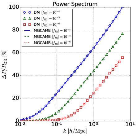
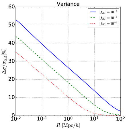
Figure 1: (Left ): Relative percent deviation in the linear matter power spectrum $P(k)$ at $z=0$ of $f(R)$ modified gravity with respect to the GR spectrum $P_{GR}(k)$ in $\Lambda$CDM. Results are shown for spectra obtained from MGCAMB (lines) as well as from evolving Eq. (6) for dark matter perturbations (open dots), for $|f_{R0}|=10^{-4}$ (blue solid line and circles), $10^{-5}$ (green dashed line and triangles) and $10^{-6}$ (red dot-dashed line and squares). (Right): Percent deviation with respect to GR of the mean square density $\sigma(R)=S(R)^{1/2}$ smoothed at scale $R$, computed from Eq. (21) at $z=0$ for the $f(R)$ model. In this case, the power spectrum was evaluated from Eq. (6).

We start by defining the linear density contrast field $\delta(R)$ smoothed on a scale $R$ around $\textbf{x}=0$

$$\delta(R)=\int\frac{d^{3}k}{(2\pi)^{3}}\tilde{\delta}(\textbf{k})\tilde{W}(k,R)\,,$$ (20)

where tildes denote quantities in Fourier space and $W(\textbf{x},R)$ is the window function that smooths the original field $\delta(\textbf{x})$ on scale $R$.

The variance $S(R)=\sigma^{2}(R)$ of the linear density field can be written as

$$S(R)=\langle|\delta(R)|^{2}\rangle=\int\frac{dk}{2\pi^{2}}k^{2}P(k)|\tilde{W}(k,R)|^{2}\,,$$ (21)

where $P(k)$ is the linear power spectrum defined via

$$\langle\tilde{\delta}(\textbf{k})\tilde{\delta}(\textbf{k}^{\prime})\rangle=(2\pi)^{3}\delta_{D}(\textbf{k}-\textbf{k}^{\prime})P(k)\,,$$ (22)

and $\delta_{D}(\textbf{k}-\textbf{k}^{\prime})$ is a Dirac delta function. Clearly the linear power spectrum will play a key role in describing the effects of modified gravity on void properties. For GR computations, we use CAMB Lewis et al. (2000) to compute the linear power spectrum. For modified gravity, we may use MGCAMB Hojjati et al. (2011); Zhao et al. (2009), a modified version of CAMB which generates the linear spectrum for a number of alternative models, such as the Hu & Sawicki $f(R)$ model Hu and Sawicki (2007) in Eq. (9) and others. However it does not compute the linear spectrum for instance for the symmetron model. Therefore we also construct the linear power spectrum independently for an arbitrary gravity theory parametrized by Eqs. (6) and  (7).

Our independent estimation of the spectrum is accomplished by evolving Eqs. (6) and (7) with parameters from specific gravity theories (e.g. Eq. (10) for $f(R)$ and Eq. (19) for symmetron models) for a set of initial conditions at matter domination. Since at sufficiently high redshifts viable gravity models reduce to GR, we take initial conditions given by CAMB at high redshifts ($z\approx 100$), when gravity is not yet modified and the Universe is deep into matter domination. We also compute initial conditions for $\dot{\delta}$ numerically by using the $\Lambda$CDM power spectrum at two closeby redshifts, e.g. at $z=99$ and $z=100$.

The results of using this procedure are shown (open dots) on the left panel of Fig. 1 and compared with the results from MGCAMB (lines) for the Hu & Sawicki model with $n=1$ and three values of the parameter $|f_{R0}|=10^{-4},10^{-5},10^{-6}$. We can see that solving Eq. (6) for the power spectrum produces results nearly identical to the full solution from MGCAMB on all scales of interest. The percent level differences may be traced to the fact that the simplified equation solved does not contain information about photons and baryons, but only dark matter. For our purposes, this procedure can be used to compute the linear power spectrum for other modified gravity models that reduce to GR at high redshifts, such as the symmetron model.

On the right panel of Fig. 1 we see that the relative difference of $\sigma(R)=S(R)^{1/2}$ for the $f(R)$ model with respect to GR can be significant on the scales of interest ($1$ Mpc/$h<R<20$ Mpc/$h$). Therefore we expect a similar impact on void properties derived from $\sigma$ and the linear power spectrum.

II.4 Spherical Collapse

Because of the void-in-cloud effect , the linearly extrapolated density contrast $\delta_{c}$ for the formation of halos is important in describing the properties of voids as both are clearly connected. Within theoretical calculations of the void abundance using the excursion set formalism, $\delta_{c}$ corresponds to another absorbing barrier, whose equivalent is not present for halo abundance. Therefore calculating $\delta_{c}$ in the gravity theory of interest gives us important hints into the properties of both halos and voids.

The computation of $\delta_{c}$ is done similarly to that of the GR case, but using Eqs. (5) and (6) with the appropriate modified gravity parameterization $\mu(k,a)$ (GR is recovered with $\mu(k,a)=1$).

Here we followed the procedure described in Pace et al. (2010). We start with appropriate initial conditions for $\delta$ and $\dot{\delta}$ and evolve the the linear Eq. (6) until $a_{c}$. The value of $\delta$ obtained is $\delta_{c}$, the density contrast linearly extrapolated for halo formation at $a=a_{c}$. In this work, since we only study simulation outputs at $z=0$, we take $a_{c}=1$ in all calculations. The only modification introduced by a nontrivial parameterization $\mu(k,a)$ is that the collapse parameters will depend on the scale $k$ of the halo. As mentioned previously, the parameterization of Eq. (7) only takes into account the evolution of the scalar field in the background , and does not account for the dependence of the collapse parameters on screening effects. Even though our calculation is approximated, it does approach the correct limits at sufficiently large and small scales.

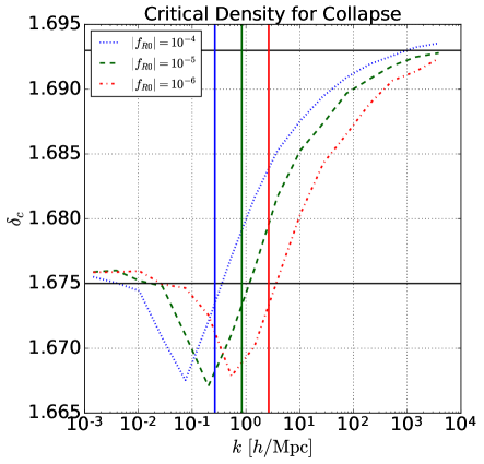
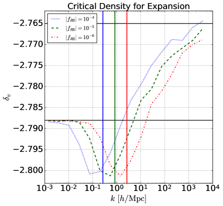
Figure 2: (Left): The critical density $\delta_{c}$ for collapse of a halo at $z=0$ as a function of halo scale $k$ in $f(R)$ modified gravity parameterized by Eq. (10) with $|f_{R0}|=10^{-4}$ (blue dotted line), $10^{-5}$ (green dashed line) and $10^{-6}$ (red dot-dashed line). The upper horizontal black line is the value expected for the strong field limit ($\mu=4/3$) and the lower line for the weak field limit, i.e. GR ($\mu=1$). The vertical lines indicate the Compton scales for each gravity with the same corresponding line colors. (Right): Same for the critical density $\delta_{v}$ for void formation at $z=0$.

For a Universe with only cold dark matter (CDM) under GR, the collapse equations can be solved analytically yielding $\delta_{c}=1.686$. For a $\Lambda$CDM Universe, still within GR, $\delta_{c}$ changes to a slightly lower value, whereas for stronger gravity it becomes slightly larger. In Fig. 2 we show $\delta_{c}$ as function of scale for the $f(R)$ model. The value of $\delta_{c}$ starts at its $\Lambda$CDM value $\delta_{c}=1.675$ on scales larger than the Compton scale ($k/a\ll m$; weak field limit where $\mu\approx 1$) and approaches the totally modified value $\delta_{c}=1.693$ on smaller scales ($k/a\gg m$; strong field limit where $\mu\approx 1+2\beta^{2}=4/3$) where the modification to the strength of gravitational force is maximal. These values were computed at the background cosmology described in § IV. They are similar to those of Schmidt et al. (2009), though the cosmology is slightly different. Note that $\delta_{c}$ reaches its strong field limit faster for larger values of $|f_{R0}|$ (value of the extra scalar field today), as expected. In the approximation of Eq. (5), $\delta_{c}$ varies with $k$ less than in the full collapse Kopp et al. (2013); Borisov et al. (2012), indicating that the no-screening approximation may not be sufficient. As a full exact calculation is beyond the scope of this work and given that $\delta_{c}$ does not change appreciably, in our abundance models we will fix $\delta_{c}$ to its $\Lambda$CDM value and encapsulate modified gravity effects on the linear power spectrum and on other model parameters.

II.5 Spherical Expansion

We now compute $\delta_{v}$, the analog of $\delta_{c}$ for voids, i.e. the density contrast linearly extrapolated to today for the formation of a void. We follow a procedure similar to spherical collapse, but in this case the initial values for $\delta_{i}$ are negative. We also set a criterium in the nonlinear field $\delta$ for the formation of a void to be $\delta_{sc}=-0.8$ or equivalently $\Delta_{sc}=1+\delta_{sc}=0.2$ Jennings et al. (2013). This quantity is somewhat the analogue for voids of the virial overdensity $\Delta_{vir}\approx 180$ for halo formation in an Einstein-de-Sitter (EdS) Universe. Despite the value of $\Delta_{vir}$ being only strictly appropriate for an EdS Universe, halos are often defined with this overdensity or other arbitrary values that may be more appropriate for specific observations. Similarly, $\delta_{sc}=-0.8$ is only strictly appropriate for shell-crossing in an EdS Universe. Here we will employ $\delta_{sc}=-0.8$, but we should keep in mind that this is an arbitrary definition of our spherical voids. When we fix this criterium for void formation we also fix the factor by which the void radius $R$ expands with respect to its linear theory radius $R_{L}$. This factor is given by $R/R_{L}=(1+\delta_{sc})^{-1/3}=1.717$ Jennings et al. (2013), and comes about from mass conservation throughout the expansion. Differently from halos, voids are not virialized structures and continue to expand faster than the background. Again environmental dependences are not incorporated in our computations as these values will depend only on scale factor $a$ and the scale $k$ or size of the void.

The right panel of Fig. 2 displays the behaviour of $\delta_{v}$ as a function of $k$, which is very similar to that of $\delta_{c}$. This is important when modelling the absorbing barriers used for evaluating the void abundance distribution function. Again the values of $\delta_{v}$ vary with $k$ less than in the full calculation Clampitt et al. (2013).

Table 1: Critical densities for the spherical collapse and expansion in the weak and strong field limits in $f(R)$ gravity.

Limit	$\mu$	$\delta_{c}$	$\delta_{v}$
Weak Field	1	1.675	-2.788
Strong Field	4/3	1.693	-2.765

In Table 1, we show the values of $\delta_{c}$ and $\delta_{v}$ in the weak and strong field limits of $f(R)$ gravity. We see that the parameters are not very much affected by the strong change in gravity ($1\%$ for $\delta_{c}$ and $0.8\%$ for $\delta_{v}$) compared with the change induced in the linear variance (see Fig. 1). Even though these collapse/expansion parameters come inside exponentials in the modeling of void abundance, these results indicate that the main contribution from gravity effects appear in the linear spectrum.

The spherical collapse and expansion calculations can be performed similarly for the symmetron model, with the appropriate change in the expression for the mass and coupling of the scalar field, as given by the Eq. (19). For $f(R)$ gravity the change in parameters does not seem to be relevant and we fix these parameters to their $\Lambda$CDM values. In order to treat both gravity models in the same way, we do the same for the symmetron model. Therefore we do not show explicit calculations of $\delta_{c}$ and $\delta_{v}$ for symmetron.

III Void Abundance Function

We now compute the void abundance distribution function as a function of void size using an extended Excursion Set formalism Maggiore and Riotto (2010a), which consists in solving the Fokker-Planck equation with appropriate boundary conditions .

Differently from the halo description, for voids it is necessary to use two boundary conditions, because of the void-in-cloud effect Sheth and van de Weygaert (2004). In this case we use two Markovian stochastic barriers with linear dependence in the density variance $S$, which is a simple generalization from the conventional problem with a constant barrier. The barriers can be described statistically as

$$\langle B_{c}(S)\rangle = \delta_{c}+\beta_{c}S\,,$$

$$\langle B_{c}(S)B_{c}(S^{\prime})\rangle = D_{c}\min(S,S^{\prime})\,,$$

$$\langle B_{v}(S)\rangle = \delta_{v}+\beta_{v}S\,,$$

$$\langle B_{v}(S)B_{v}(S^{\prime})\rangle = D_{v}\min(S,S^{\prime})\,,$$ (23)

where $B_{c}(S)$ is the barrier associated with halos and $B_{v}(S)$ the barrier associated with voids. Notice that the two barriers are uncorrelated, i.e. $\langle B_{c}(S)B_{v}(S^{\prime})\rangle=0$. Here $\beta_{c}$ describes the linear relation between the mean barrier and the variance $S$, $\delta_{c,v}$ is the mean barrier as $S\rightarrow 0$ ($R\rightarrow\infty$), and $D_{c,v}$ describes the barrier diffusion coefficient.

As we consider different scales $R$, the smoothed density field $\delta(R)$ performs a random walk with respect to a time coordinate $S$, and we have

$$\langle\delta(S)\rangle = 0\,,$$

$$\langle\delta(S)\delta(S^{\prime})\rangle = \min(S,S^{\prime})\,.$$ (24)

The field $\delta$ satisfies a Langevin equation with white noise and therefore the probability density $\Pi(\delta,S)$ to find the value $\delta$ at variance $S$ is a solution of the Fokker-Planck equation

$$\frac{\partial\Pi}{\partial S}=\frac{1}{2}\frac{\partial^{2}\Pi}{\partial\delta^{2}}\,,$$ (25)

with boundary conditions

$$\Pi(\delta=B_{c}(S),S)=0\quad\mbox{and}\quad\Pi(\delta=B_{v}(S),S)=0\,,$$ (26)

and initial condition

$$\Pi(\delta,S=0)=\delta_{D}(\delta)\,,$$ (27)

where $\delta_{D}$ is a Dirac delta function and notice that $S\rightarrow 0$ corresponds to void radius $R\rightarrow\infty$. In order to solve this problem, it is convenient to introduce the variable Corasaniti and Achitouv (2011a)

$$Y(S)=B_{v}(S)-\delta(S)\,.$$ (28)

Making the simplifying assumption that $\beta\equiv\beta_{c}=\beta_{v}$ and using the fact that all variances can be added in quadrature, the Fokker-Planck Eq. (25) becomes

$$\frac{\partial\Pi}{\partial S}=-\beta\frac{\partial\Pi}{\partial Y}+\frac{1+D}{2}\frac{\partial^{2}\Pi}{\partial Y^{2}}$$ (29)

where $D=D_{v}+D_{c}$.

We define $\delta_{T}=|\delta_{v}|+\delta_{c}$ and notice that $\delta(S)=B_{v}(S)$ implies $Y(S)=0$, $\delta(S)=B_{c}(S)$ implies $Y(S)=-\delta_{T}$ (only occurs because we set $\beta_{c}=\beta_{v}$) and $\delta(0)=0$ implies $Y(0)=\delta_{v}$. Therefore the boundary conditions become

$$\Pi(Y=0,S)=0\quad\mbox{and}\quad\Pi(Y=-\delta_{T},S)=0\,,$$ (30)

and the initial conditions

$$\Pi(Y,0)=\delta_{D}(Y-\delta_{v})\,.$$ (31)

Rescaling the variable $Y\rightarrow\tilde{Y}=Y/\sqrt{1+D}$ and factoring the solution in the form $\Pi(\tilde{Y},S)=U(\tilde{Y},S)\exp[c(\tilde{Y}-cS/2-\tilde{Y}_{0})]$ where $c=\beta/\sqrt{1+D}$ and $\tilde{Y}_{0}=\delta_{v}/\sqrt{1+D}$. The function $U(\tilde{Y},S)$ obeys a Fokker-Planck equation like Eq. (25), for which the solution is known Sheth and van de Weygaert (2004). Putting it all together the probability distribution function becomes

$$\Pi(Y,S) = \exp\left[\frac{\beta}{1+D}\left(Y-\frac{\beta S}{2}-\delta_{v}\right)\right]$$

$$\times\sum_{n=1}^{\infty}\frac{2}{\delta_{T}}\sin\left(\frac{n\pi\delta_{v}}{\delta_{T}}\right)\sin\left(\frac{n\pi}{\delta_{T}}Y\right)\exp\left[-\frac{n^{2}\pi^{2}(1+D)}{2\delta_{T}^{2}}S\right]\,.$$

The ratio of walkers that cross the barrier $B_{v}(S)$ is then given by

$$\mathcal{F}(S)=\frac{\partial}{\partial S}\int_{\infty}^{0}dY\Pi(Y,S)=\frac{1+D}{2}\left.\frac{\partial\Pi}{\partial Y}\right|_{Y=0}\,,$$ (33)

where we used the modified Fokker-Planck equation Eq. (29) and the first boundary condition from Eq. (30). The void abundance function, defined as $f(S)=2S\mathcal{F}(S)$, for this model is then given by

$$f(S) = 2(1+D)\exp\left[-\frac{\beta^{2}S}{2(1+D)}+\frac{\beta\delta_{v}}{(1+D)}\right]$$

$$\times \sum_{n=1}^{\infty}\frac{n\pi}{\delta_{T}^{2}}S\sin\left(\frac{n\pi\delta_{v}}{\delta_{T}}\right)\exp\left[-\frac{n^{2}\pi^{2}(1+D)}{2\delta_{T}^{2}}S\right]$$

There are four important limiting cases to consider:

• $D=\beta=0$: This is the simplest case of two static barries. The expression in this case was first obtained in Sheth and van de Weygaert (2004) and compared to simulations in Jennings et al. (2013). It is given by

  $$f_{D=\beta=0}(S) = 2\sum_{n=1}^{\infty}\frac{n\pi}{\delta_{T}^{2}}S\sin\left(\frac{n\pi\delta_{v}}{\delta_{T}}\right)$$ (35)

  $$\times \exp\left(-\frac{n^{2}\pi^{2}}{2\delta_{T}^{2}}S\right)\,,$$

  This is one of the functional forms tested in this work and the only case with no free parameters. We refer to this case as that of 2 static barriers (2SB).

• $D=0$ and $\beta\neq 0$: This case considers that the barriers depend linearly on $S$ but are not difusive. In this case the expression is given by

  $$f_{D=0}(S) = 2e^{-\frac{\beta^{2}S}{2}}e^{\beta\delta_{v}}\sum_{n=1}^{\infty}\frac{n\pi}{\delta_{T}^{2}}S\sin\left(\frac{n\pi\delta_{v}}{\delta_{T}}\right)$$ (36)

  $$\times \exp\left(-\frac{n^{2}\pi^{2}}{2\delta_{T}^{2}}S\right)$$

  This expression recovers Eq. (C10) from Sheth and van de Weygaert (2004). Note that these authors define the barrier with a negative slope, therefore our $\beta$ is equal to their $-\beta$, but $\delta_{v}<0$ in our case;

• $\beta=0$ and $D\neq 0$: Here we have a barrier that does not depend on $S$ but which is diffusive. In this case we have

  $$f_{\beta=0}(S) = 2(1+D)\sum_{n=1}^{\infty}\frac{n\pi}{\delta_{T}^{2}}S\sin\left(\frac{n\pi\delta_{v}}{\delta_{T}}\right)$$ (37)

  $$\times \exp\left(-\frac{n^{2}\pi^{2}(1+D)}{2\delta_{T}^{2}}S\right)$$

  This expression is the same as the original formula from Sheth and van de Weygaert (2004), but changing $S\rightarrow(1+D)S$ or $(\delta_{v},\delta_{v})\rightarrow(\delta_{v},\delta_{c})/\sqrt{1+D}$, as expected when the constant barrier becomes diffusive Maggiore and Riotto (2010b);
  

• Large void radius: As discussed in Sheth and van de Weygaert (2004) and Jennings et al. (2013), for large radii $R$ the void-in-cloud effect is not important as we do not expected to find big voids inside halos. In others words, when $S\rightarrow 0(R\rightarrow\infty)$ the abundance becomes equal to that of a one-barrier problem. Even though we do not attempt to properly consider the limit of Eq. (LABEL:my) when $S\rightarrow 0$, this expression can be directly compared to the function of the problem with one linear diffusive barrier (1LDB), given by Corasaniti and Achitouv (2011b)

  $$f_{1{\rm LDB}}(S)=\frac{|\delta_{v}|}{\sqrt{S(1+D_{v})}}\sqrt{\frac{2}{\pi}}\exp\left[-\frac{(|\delta_{v}|+\beta_{v}S)^{2}}{2S(1+D_{v})}\right]$$ (38)

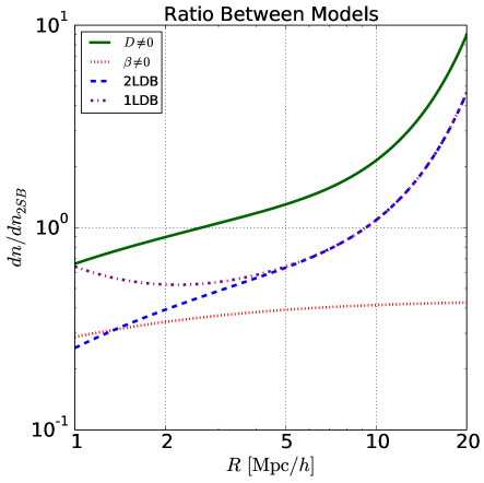
Figure 3: Ratio of multiple models for void abundance relative to the model with two static barriers (2SB) Eq. (35) ($\beta=D=0$). We show models with only $D\neq 0$ (green solid line), with only $\beta\neq 0$ (red dotted line), the 1LDB model (purple dotted-dashed line) and the 2LDB model (blue dashed line). The latter two cases are the main models considered in this work and differ only at small radii ($R\lesssim 4$ Mpc$/h$), as a manifestation of the void-in-cloud effect.

In Fig. 3, we compare the void abundance from multiple cases by taking their ratio with respect to the abundance of the 2SB model. The abundance of the model with $D\neq 0$ is substantially higher than 2SB, whereas that of the model with $\beta\neq 0$ is significantly lower. The cases with two linear diffusive barriers (2LDB) Eq. (LABEL:my) and one linear diffusive barrier (1LDB) Eq. (38) are the main models considered in this work. The void abundance of the 1LDB and 2LDB models are nearly identical for $R>4$ Mpc/$h$, when the same values of $\beta$ and $D$ are used. Table 2 summarizes the properties of the three main models considered and how they generalize each other.

Table 2: Abundance models for voids considered in this work. Voids require two barriers to avoid the void-in-cloud effect.

Model	Barriers	Nonzero Params	Equation
2SB	2 (static)	$\delta_{c}$, $\delta_{v}$	Eq.(35)
1LDB	1 (linear+diffusive)	$\delta_{v}$, $\beta_{v}$, $D_{v}$	Eq.(38)
2LDB	2 (linear+diffusive)	$\delta_{c}$, $\delta_{v}$, $\beta$, $D$	Eq.(LABEL:my)

Given the ratio of walkers that cross the barrier $B_{v}(S)$ with a radius given by $S(R)$, the number density of voids with radius between $R_{L}$ and $R_{L}+dR_{L}$ in linear theory is given by

$$\frac{dn_{L}}{d\ln R_{L}}=\left.\frac{f(\sigma)}{V(R_{L})}\frac{d\ln\sigma^{-1}}{d\ln R_{L}}\right|_{R_{L}(R)}$$ (39)

where the subscript $L$ denotes linear theory quantities, $V(R_{L})$ is the volume of the spherical void of linear radius $R_{L}$ and recall $S=\sigma^{2}$.

Whereas for halos the number density in linear theory is equal to the final nonlinear number density, for voids this is not the case. In fact, Jennings et al. Jennings et al. (2013) shows that such criterium produces nonphysical void abundances, in which the volume fraction of the Universe occupied by voids becomes larger than unity. Instead, to ensure that the void volume fraction is physical (less than unity) the authors of Jennings et al. (2013) impose that the volume density is the conserved quantity when going from the linear-theory calculation to the nonlinear abundance. Therefore, when a void expands from $R_{L}\rightarrow R$ it combines with its neighbours to conserve volume and not number. This assumption is quantified by the equation

$$V(R)dn=\left.V(R_{L})dn_{L}\right|_{R_{L}(R)}\,,$$ (40)

which implies

$$\frac{dn}{d\ln R}=\left.\frac{f(\sigma)}{V(R)}\frac{d\ln\sigma^{-1}}{d\ln R_{L}}\frac{d\ln R_{L}}{d\ln R}\right|_{R_{L}(R)}\,,$$ (41)

where recall in our case $R=(1+\delta_{sc})^{-1/3}R_{L}=1.717R_{L}$ is the expansion factor for voids. Therefore we have trivially $d\ln R_{L}/d\ln R=1$ above.

The expression in Eq. (41) – referred as the Vdn model – along with the function in Eq. (LABEL:my) provide the theoretical prediction for the void abundance distribution in terms of void radius, which will be compared to the abundance of spherical voids found in N-body simulations of GR and modified gravity.

IV Voids from Simulations

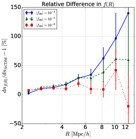
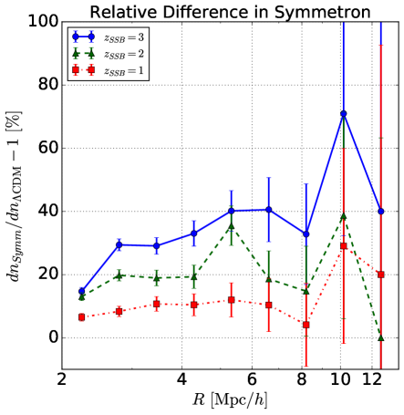
Figure 4: Relative difference between void abundance in modified gravity models and in standard GR ($\Lambda$CDM model). (Left): Relative difference of $f(R)$ theories, for parameters $|f_{R0}|=10^{-6}$ (red squares with dotted-dashed line), $10^{-5}$ (green triangles with dashed line) and $10^{-4}$ (blue circles with solid line). (Right): Relative difference of symmetron theories, for parameters $z_{SSB}=1$ (red squares with dotted-dashed line), $2$ (green triangles with dashed line) and $3$ (blue circles with solid line).

We used the N-body simulations that were run with the Isis code Llinares et al. (2014) for $\Lambda$CDM, $f(R)$ Hu-Sawicki and symmetron cosmological models. For the $f(R)$ case we fixed $n=1$ and considered $|f_{R0}|=10^{-4}$, $10^{-5}$ and $10^{-6}$. For symmetron, we fix $\beta_{0}=1$ and $L=1$ and used simulations SymmA, SymmB, SymmD, which have $z_{SSB}=1,2,3$ respectively. Each simulation has $512^{3}$ particles in a box of size $256$ Mpc/$h$, and cosmological parameters $(\Omega_{b},\Omega_{dm},\Omega_{\Lambda},\Omega_{\nu},h,T_{CMB},n_{s},\sigma_{8})=(0.045,0.222,0.733,0.0,0.72,2.726{\rm K},1.0,0.8)$. These represent the baryon density relative to critical, dark matter density, effective cosmological constant density, neutrino density, Hubble constant, CMB temperature, scalar spectrum index and spectrum normalization. The normalization is actually fixed at high redshifts, so that $\sigma_{8}=0.8$ is derived for the $\Lambda$CDM simulation, but is larger for the modified gravity simulations. In terms of spatial resolution, seven levels of refinement were employed on top of a uniform grid with 512 nodes per dimension. This gives an effective resolution of of 32,678 nodes per dimension, which corresponds to 7.8 kpc/$h$. The particle mass is $9.26\times 10^{9}M_{\odot}/h$.

We ran the ZOBOV void-finder algorithm Neyrinck (2008) – based on Voronoi tessellation – on the simulation outputs at $z=0$ in order to find underdense regions and define voids, and compared our findings to the Vdn model of Eq. (41) Jennings et al. (2013) with the various multiplicity functions $f(\sigma)$ proposed above (2SB, 1LDB and 2LDB models).

First, we used ZOBOV to determine the position of the density minima locations within the simulations and rank them by signal-to-noise S/N significance. Next, we started from the minimum density point of highest significance and grew a sphere around this point, adding one particle at a time in each step, until the overdensity $\Delta=1+\delta$ enclosed within the sphere was $0.2$ times the mean background density of the simulation at $z=0$. Therefore we defined spherical voids, which are more closely related to our theoretical predictions based on spherical expansion.

We also considered growing voids around the center-of-volume from the central Voronoi zones. The center-of-volume is defined similarly to the center-of-mass, but each particle position is weighted by the volume of the Voronoi cell enclosing the particle, instead of the particle mass. Using the center-of-volume produces results very similar to the previous prescription, so we only present results for the centers fixed at the density minima.

In Fig. 4 we compare the void abundance inferred from simulations for the three $f(R)$ and the three symmetron theories relative to the $\Lambda$CDM model. Since the differential abundance as a function of void radius is denoted by $dn/d\ln R$, we denote the relative difference between the $f(R)$ and $\Lambda$CDM abundances by $dn_{f(R)}/dn_{\Lambda{\rm CDM}}-1$ and show the results in terms of percent differences. The error bars shown here reflect shot-noise from voids counts in the simulation runs. In the $f(R)$ simulation this relative difference is around $100\%$ at radii $R>10$ Mpc$/h$ (for the $|f_{R0}|=10^{-4}$ case). In the symmetron simulation, the difference is around $40\%$ (for the $z_{SSB}=3$ case), for radii $R\sim 8$ Mpc$/h$. This indicates that void abundance is a potentially powerful tool for constraining modified gravity parameters.

V Results

V.1 Fitting $\beta$ and $D$ from Simulations

In order to use the theoretical expression in Eq. (LABEL:my) to predict the void abundance we need values for the parameters $\beta$ and $D$. The usual interpretation of $\beta$ is that it encodes, at the linear level, the fact that the true barrier in real cases is not constant. In other words, the contrast density for the void (or halo) formation depends on its size/scale. This can occur because halos/voids are not perfectly spherical and/or because the expansion (or collapse) intrinsically depends on scale (Birkhoff’s theorem is generally not valid in modified gravity). The scale dependency induced by modified gravity can be calculated using our model for spherical collapse (expansion), described in sections II.C and II.D, by fitting a linear relationship between $\delta_{c}$ ($\delta_{v}$) or average barrier $\langle B_{c}\rangle$ ($\langle B_{v}\rangle$) as a function of the variance $S(R)$. Here we use $k=2\pi/R$ to convert wave number to scale $R$.

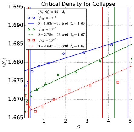
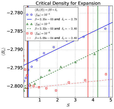
Figure 5: (Left): Average barrier $\langle B_{c}\rangle$ for halos as a function of variance $S$, for the $f(R)$ parameters: $|f_{R0}|=10^{-6}$ (red squares), $10^{-5}$ (green triangles) and $10^{-4}$ (blue circles), and corresponding fits for each case in same colors and with dotted-dashed, dashed and solid lines respectively. Vertical lines indicate the limits used for the fits, which also correspond to the range of interest for the study of voids in our case ($2.0-14.0$ Mpc/$h$). (Right): Same for the void barrier $\langle B_{v}\rangle$.

In Fig. 5 we show the average barriers $\langle B_{c}\rangle$ , $\langle B_{v}\rangle$ as functions of variance $S$ for multiple gravity theories, and empirical fits for the parameters $\delta_{c},\delta_{v},\beta_{c},\beta_{v}$ from Eqs. (23). These fits indicate that the barriers depend weakly on scale in the range of interest. The values of $\delta_{c},\delta_{v}$ are nearly constant and those of $\beta_{c},\beta_{v}$ are of order $10^{-3}$ while the corresponding values for halos in $\Lambda$CDM are of order $10^{-1}$ Achitouv and Corasaniti (2012). Even though voids are quite spherical, the small values of $\beta$ indicate that the main contribution to $\beta$ may come from more general aspects of nonspherical evolution. The small fitted values of $\beta$ can also be due to errors induced by the approximations in the nonlinear equation Eq. (5), which does not capture screening effects of modified gravity.

Given these issues, and as it is beyond the scope of this work to consider more general collapse models or study the exact modified gravity equations, we will instead keep the values of $\delta_{c}$ and $\delta_{v}$ fixed to their $\Lambda$CDM values and treat $\beta$ as a free parameter to be fitted from the abundance of voids detected in the simulations.

Likewise, the usual interpretation of $D$ is that it encodes stochastic effects of possible problems in our void (halo) finder Maggiore and Riotto (2010b), such as an intrinsic incompleteness or impurity of the void sample, or other peculiarities of the finder, which may even differ from one algorithm to another. Therefore $D$ is also taken as a free parameter in our abundance models.

We jointly fit for the parameters $\beta$ and $D$ using the voids detected in the N-body simulations described in §IV, with the values of $\delta_{c}$ and $\delta_{v}$ fixed to their $\Lambda$CDM values (the non-constant barrier introduced by modified gravity is therefore encoded by $\beta$).

We use the emcee algorithm Foreman-Mackey et al. (2013) to produce a Monte Carlo Markov Chain (MCMC) and map the posterior distribution of these parameters. The results for these fits using the 2LDB model Eq. (LABEL:my) the 1LDB model Eq. (38) are shown in Table 3, for $f(R)$ and symmetron gravity. The table shows the mean values and 1$\sigma$ errors around the mean, as inferred from the marginalized posteriors.

Table 3: Mean values and $1\sigma$ errors for $\beta$ and $D$, fitted from void abundance in N-body simulations for GR, $f(R)$ and symmetron gravity and for the 1LDB and 2LDB models of void abundance. For 1LDB, $\beta=\beta_{v}$ and $D=D_{v}$. For 2LDB, $\beta=\beta_{c}=\beta_{v}$ and $D=D_{c}+D_{v}$.

Gravity	Parameter	Model	$\beta$	$D$
GR	-	1LDB	$0.016^{0.004}_{0.004}$	$0.185^{0.021}_{0.021}$
$f(R)$	$|f_{R0}|=10^{-6}$	1LDB	$0.029^{0.033}_{0.032}$	$0.168^{0.020}_{0.021}$
$f(R)$	$|f_{R0}|=10^{-5}$	1LDB	$0.034^{0.003}_{0.003}$	$0.146^{0.021}_{0.021}$
$f(R)$	$|f_{R0}|=10^{-4}$	1LDB	$0.044^{0.003}_{0.003}$	$0.076^{0.021}_{0.021}$
symmetron	$z_{SSB}=1$	1LDB	$0.010^{0.003}_{0.003}$	$0.150^{0.020}_{0.020}$
symmetron	$z_{SSB}=2$	1LDB	$0.025^{0.002}_{0.002}$	$-0.011^{0.016}_{0.017}$
symmetron	$z_{SSB}=3$	1LDB	$0.034^{0.002}_{0.002}$	$-0.149^{0.014}_{0.014}$
GR	-	2LDB	$-0.034^{0.002}_{0.002}$	$0.057^{0.014}_{0.014}$
$f(R)$	$|f_{R0}|=10^{-6}$	2LDB	$-0.032^{0.002}_{0.002}$	$-0.003^{0.012}_{0.011}$
$f(R)$	$|f_{R0}|=10^{-5}$	2LDB	$-0.030^{0.002}_{0.002}$	$-0.065^{0.011}_{0.012}$
$f(R)$	$|f_{R0}|=10^{-4}$	2LDB	$-0.026^{0.002}_{0.002}$	$-0.155^{0.010}_{0.010}$
symmetron	$z_{SSB}=1$	2LDB	$-0.045^{0.002}_{0.002}$	$0.001^{0.012}_{0.012}$
symmetron	$z_{SSB}=2$	2LDB	$-0.032^{0.002}_{0.002}$	$-0.185^{0.009}_{0.009}$
symmetron	$z_{SSB}=3$	2LDB	$-0.024^{0.001}_{0.001}$	$-0.347^{0.006}_{0.006}$

In Fig. 6 we show the abundance of voids $dn/d\ln R$ as measured from simulations (open dots), as well as three theoretical models, namely the 2SBJennings et al. (2013), 1LDB Eq. (38) and 2LDB Eq. (LABEL:my) models. Multiple panels show results for $\Lambda$CDM and $f(R)$ models. In Fig. 7 we show the same for $\Lambda$CDM and symmetron models.

We can see that linear-diffusive-barrier models (1LDB and 2LDB) work best in all gravities, relative to the static barriers model (2SB). In fact, these two models describe the void abundance distribution within $10\%$ precision for $R\lesssim 10$ Mpc/$h$. As expected, the model with two linear diffusive barriers (2LDB) better describes the abundance of small voids ($R\lesssim 3$ Mpc/$h$), due to the void-in-cloud effect, more relevant for small voids Sheth and van de Weygaert (2004).

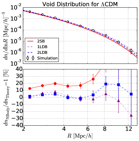
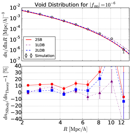
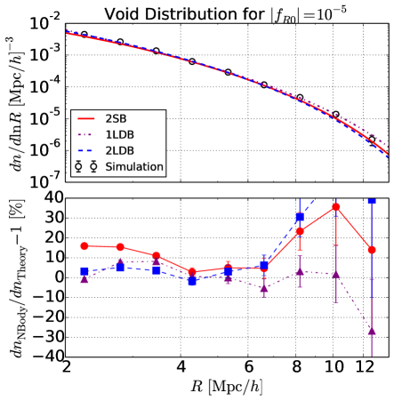
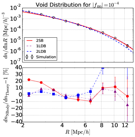
Figure 6: (Top Left): The upper sub-panel shows the void differential abundance distribution $dn/d\ln R$ as a function of void radius $R$ for GR ($\Lambda$CDM) from simulations (open dots), along with theory predictions from the 2SB model Jennings et al. (2013) (red solid curve), from the 1LDB Eq. (38) (purple dotted-dashed curve) and the 2LDB model Eq. (LABEL:my) (blue dashed line). The lower sub-panel shows the relative difference between simulation data and each theory model. (Top Right): Same for $f(R)$ modified gravity with $|f_{R0}|=10^{-6}$. (Bottom Left): Same for $|f_{R0}|=10^{-5}$ (Bottom Right): Same for $|f_{R0}|=10^{-4}$

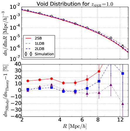
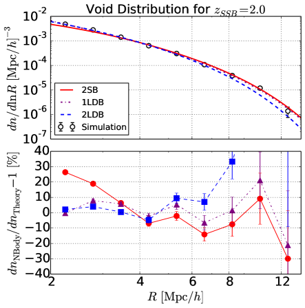
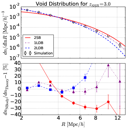
Figure 7: Same as Fig. 6, but for the symmetron model with $z_{SSB}=1$ (top right), $2$ (bottom left) and $3$ (bottom right).

In Table 4 we show the reduced $\chi^{2}$ for GR, the three $f(R)$ models and three symmetron models, This shows again that models with linear diffusive barriers provide a better fit to the simulation data – with $\chi^{2}$ one order of magnitude smaller – and that the 2LDB model gives the overall best fits. Another interesting feature for the main model presented in this work (2LDB) is that its reduced $\chi^{2}$ grows with the intensity of modified gravity. This may indicate that, despite being the best model considered, it may not capture all important features in modified gravity at all orders. We also find that the $f(R)$ model is better fitted than the symmetron model. Since the linear treatment is the same for both gravity models, the 2LDB model may be more appropriate to describe the chameleon screening of $f(R)$ than symmetron screening. Nonetheless, the 2LDB model provides a reasonable representation of the data from both gravity theories in the range considered here.

Table 4: Reduced $\chi^{2}$ for each gravity model and for the three models of void abundance considered.

Gravity	2SB	1LDB	2LDB
GR	15.76	3.45	1.59
$|f_{R0}|=10^{-6}$	13.10	3.97	1.67
$|f_{R0}|=10^{-5}$	21.10	5.52	2.11
$|f_{R0}|=10^{-4}$	34.86	5.66	2.78
$z_{SSB}=1$	22.20	3.64	1.12
$z_{SSB}=2$	49.06	4.75	2.57
$z_{SSB}=3$	209.05	8.10	4.77

As both parameters $\beta$ and $D$ have an explicit dependence on the modified gravity strength, next we fit a relationship between the abundance parameters $\beta$ and $D$ and the gravity parameters $\log_{10}|f_{R0}|$ and $z_{SSB}$. In these fits we set the value $\log_{10}|f_{R0}|=-8$ to represent the case of $\Lambda$CDM cosmology, as this is indeed nearly identical to $\Lambda$CDM for purposes of large-scale structure observables, i.e. $\log_{10}|f_{R0}|=-8\simeq-\infty$.

As we expect $\beta$ and $D$ to depend monotonically on the modified gravity parameters, we fit for them using simple two-parameter functions. For $\beta$ case we use a straight line, and for $D$ a second order polynomial with maximum fixed by the $\Lambda$CDM value. These fits are shown in the multiple panels of Fig. 8.

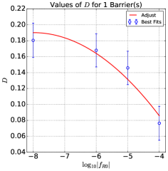
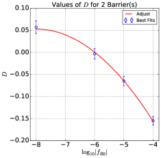
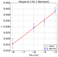
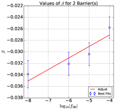
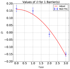
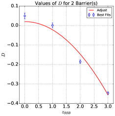
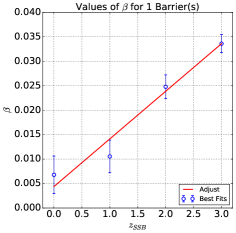
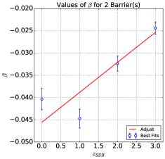
Figure 8: (Top Row): Fits of $D$ and $\beta$ as a function of $\log_{10}|f_{R0}|$ in $f(R)$ gravity. These fits are shown for $D$ in the 1LDB and 2LDB models, and for $\beta$ in the 1LDB and 2LDB models respectively from left to right. (Bottom Row): Same for fits as a function of $z_{SSB}$ in symmetron gravity.

Our values of $\beta$ and $D$ as a function of gravity parameters fluctuate considerably around the best fit. This occurs at least partially because we have used only one simulation for each gravity model, and we expect this oscillation to be reduced with a larger number of simulations. At present, the use of the fits is likely more robust than the use of exact values obtained for each parameter/case.

V.2 Constraining Modified Gravity

Given the fits for $\beta$ and $D$ obtained in the last subsection, we now check for the power of constraining modified gravity from the void distribution function in each of the three void abundance models considered, namely 2SB, 1LDB and 2LDB. We take the abundance of voids actually found in simulations (described in the §IV) to represent a hypothetical real measurement of voids and compare it to the model predictions, evaluating the posterior for $\log_{10}|f_{R0}|$ and $z_{SSB}$, thus assessing the constraining power of each abundance model in each gravity theory. Obviously the constraints obtained in this comparison are optimistic – since we are taking as real data the same simulations used to fit for the abundance model parameters – but they provide us with idealized constraints similar in spirit to a Fisher analysis around a fiducial model.

The posteriors for the gravity parameters are shown in Figs. 9 and 10, as well as the mean values and 1$\sigma$ errors in each case. For the results shown here all cosmological parameters from § IV have been fixed to their true values. We also considered the case where we apply Planck priors Planck Collaboration et al. (2015) on $\Omega_{dm}$ and $h$ and let them vary freely in the MCMC, keeping other parameters fixed. In the latter case, the mean values and errors found for $\log_{10}|f_{R0}|$ are slightly worse, but the errors remain less than twice those found for the case of all fixed parameters. Moreover, the errors derived for $\Omega_{dm}$ and $h$ reduce to half of their original Planck priors.

In Fig. 9 we can see that the 2SB model predicts values for the $f(R)$ parameter ($\log_{10}|f_{R0}|$) which are incorrect by more than 3$\sigma$ for all cases. In fact, this model predicts incorrect values even for general relativity. This is not surprising given the bad $\chi^{2}$ fits from Table IV. Therefore we find this model to be highly inappropriate to describe the abundance of dark matter voids, and focus on models with linear diffusive barriers.

Both the 1LDB and 2LDB models predict correct values for the gravity parameters within 1$\sigma$ in most cases. We find that the 1LDB model presents results similar to 2LDB, despite being a simpler model and providing a worse fit to the data (larger reduced $\chi^{2}$). For $\Lambda$CDM both posteriors go to $\log_{10}|f_{R0}|=10^{-8}$, which represents the GR case by assumption. This shows that within the $f(R)$ framework, we can also constrain GR with reasonable precision from void abundance, using one of these two abundance models with diffusive barriers (1LDB, 2LDB).

For the symmetron Model, we can see in Fig. 10 that the parameter $z_{SSB}$ is also well constrained, similarly to $f_{R0}$ in $f(R)$. Again the 2SB model has the worst result in all cases, and the 1LDB and 2LDB models produce similar results.

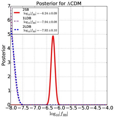
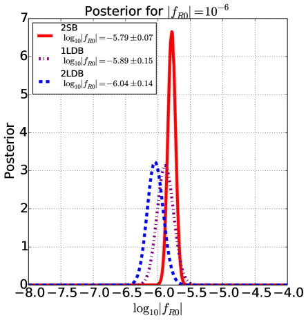
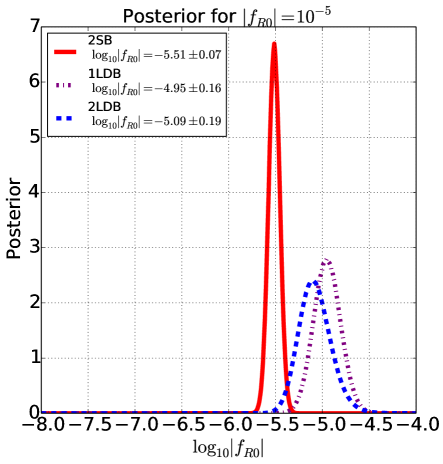
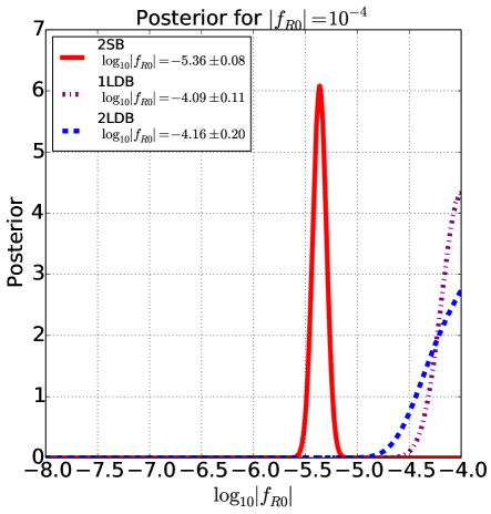
Figure 9: Posterior distribution for $\log_{10}|f_{R0}|$ and for the three abundance models considered in the text, 2SB model Jennings et al. (2013) (red continuous line), 2LDB model Eq. (LABEL:my) (blue dashed line) and 1LDB model Eq. (38) (purple dotted dashed line). The mean and 1$\sigma$ values of $\log_{10}|f_{R0}|$ in each case are indicated in the legend. (Top Left): Posterior for the $\Lambda$CDM simulation. (Top Right): Posterior for the $|f_{R0}|=10^{-6}$. (Bottom Left): Posterior for the $|f_{R0}|=10^{-5}$. (Bottom Right): Posterior for the $|f_{R0}|=10^{-4}$.

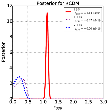
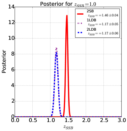
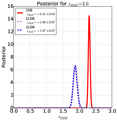
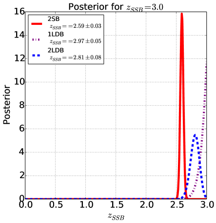
Figure 10: Same as Fig. 9, but for the symmetron model with $z_{SSB}=1$ (top right), 2 (bottom left) and 3 (bottom right).

In Table 5 we show the best-fit values, mean values and 1$\sigma$ errors from the posteriors distributions of Figs. 9, 10 for the $f(R)$ and symmetron theories. It becomes again clear that our proposed models with linear diffusive barriers (1LDB and 2LDB) give results much closer to the correct true values, compared to the original static barriers case 2SB Jennings et al. (2013). In particular, the 2LDB is within 1-3$\sigma$ concordance for all cases.

Table 5: Values for best-fit, mean and $1\sigma$ errors in the modified gravity parameters ($f_{R0}$ and $z_{SSB}$) for the three void abundance models 2SB, 1LDB and 2LDB.

Gravity parameters	Best-Fit			Mean $\pm$ ($1\sigma$ error)
	2SB	1LDB	2LDB	2SB	1LDB	2LDB
$\log_{10}|f_{R0}|=-8$ ($\Lambda$CDM)	-6.24	-8.00	-8.00	-6.24$\pm$0.09	-7.94$\pm$0.08	-7.92$\pm$0.10
$\log_{10}|f_{R0}|=-6$	-5.78	-5.88	-6.04	-5.79$\pm$0.07	-5.89$\pm$0.15	-6.04$\pm$0.14
$\log_{10}|f_{R0}|=-5$	-5.51	-4.95	-5.10	-5.51$\pm$0.07	-4.95$\pm$0.16	-5.09$\pm$0.19
$\log_{10}|f_{R0}|=-4$	-5.36	-4.01	-4.00	-5.36$\pm$0.08	-4.09$\pm$0.11	-4.16$\pm$0.20
$z_{SSB}=0$ ($\Lambda$CDM)	1.14	0.32	0.21	1.14$\pm$0.04	0.27$\pm$0.19	0.20$\pm$0.16
$z_{SSB}=1$	1.46	1.17	1.16	1.46$\pm$0.03	1.17$\pm$0.05	1.17$\pm$0.06
$z_{SSB}=2$	1.63	1.89	1.88	2.31$\pm$0.03	1.89$\pm$0.07	1.87$\pm$0.07
$z_{SSB}=3$	1.77	3.00	2.81	2.59$\pm$0.03	2.97$\pm$0.05	2.81$\pm$0.08

V.3 Voids in Galaxy Samples

In real observations it is much harder to have direct access to the the dark matter density field. Instead we observe the galaxy field, a biased tracer of the dark matter. Therefore it is important to investigate the abundance of voids defined by galaxies and the possibility of constraining cosmology and modified gravity in this case.

We introduce galaxies in the original dark matter simulations using the Halo Occupation Distribution (HOD) model from Zheng et al. (2007). In Nadathur and Hotchkiss (2015b) the authors investigated similar void properties but did not considered spherical voids, using instead the direct outputs of the VIDE Sutter et al. (2015) void finder.

In our implementation, first we find the dark matter halos in the simulations using the overdensities outputted by ZOBOV. We grow a sphere around each of the densest particles until its enclosed density is $200$ times the mean density of the simulation. This process is the reverse analog of the spherical void finder described in § IV, the only difference being the criterium used to sort the list of potential halo centers. Here we sort them using the value of the point density, not a S/N significance, as the latter is not provided by ZOBOV in the case of halos.

We populate these halos with galaxies using the HOD model of Zheng et al. (2007). This model consist of a mean occupation function of central galaxies given by

$$\langle N_{cen}(M)\rangle=\frac{1}{2}\left[1+{\rm erf}\left(\frac{\log M-\log M_{min}}{\sigma_{\log M}}\right)\right],$$ (42)

with a nearest-integer distribution. The satellite galaxies follow a Poisson distribution with mean given by

$$\langle N_{sat}(M)\rangle=\langle N_{cen}(M)\rangle\left(\frac{M-M_{0}}{M_{1}^{\prime}}\right)^{\alpha}.$$ (43)

Central galaxies are put in the center of halo, and the satellite galaxies are distributed following a Navarro Frenk and White ((NFW), Navarro et al., 1996) profile.

We use parameter values representing the sample Main 1 of Nadathur and Hotchkiss (2015b), namely: $(\log M_{min},\sigma_{\log M},\log M_{0},\log M_{1}^{\prime},\alpha)=(12.14,0.17,11.62,13.43,1.15)$. These parameters give a mock galaxy catalogue with galaxy bias $b_{g}=1.3$ and mean galaxy density $\bar{n}_{g}=5.55\times 10^{-3}(h/$Mpc$)^{3}$ in $\Lambda$CDM.

We then find voids in this galaxy catalogue using the same algorithm applied to the dark matter catalogue (described in § IV). We use the same criterium that a void is a spherical, non-overlapping structure with overdensity equal to $0.2$ times the background galaxy density. However, as the galaxies are a biased tracer of the dark matter field, if we find galaxy voids with $0.2$ times the mean density, we are really finding regions which are denser in the dark matter field. In fact, if $\delta_{g}=b_{g}\delta$ is the galaxy overdensity, with galaxy bias $b_{g}$ and $\delta$ is the dark matter overdensity we have

$$\Delta=1+\delta=1+\frac{\delta_{g}}{b_{g}},$$ (44)

Therefore, if we find voids with $\delta_{g}=-0.8$ and $b_{g}=1.3$ we have $\Delta=0.38$, i.e. the galaxy voids enclose a region of density $0.38$ times the mean density of the dark matter field. Therefore it is this value that must be used in the previous theoretical predictions.

Using this value, the relation between linear and nonlinear radii is $R=1.37R_{L}$, and the density parameter for the spherical void formation – calculated using the spherical expansion equations (§ II.D) – is $\delta_{v}=-1.33$. We insert these new values into the theoretical predictions and compare to the measured galaxy void abundance. The result is shown in Fig. 11 for the $\Lambda$CDM case. We see that both original models, 2SB and 2LDB (blue curves), with $R=1.71R_{L}$ and $\delta_{v}=-2.788$, provide incorrect predictions for the abundance of galaxy voids. However when corrected for the galaxy bias (red curves), these models are in good agreement with the data. We also see that the 2LDB provides a slightly better fit, which is not significant given the error bars.

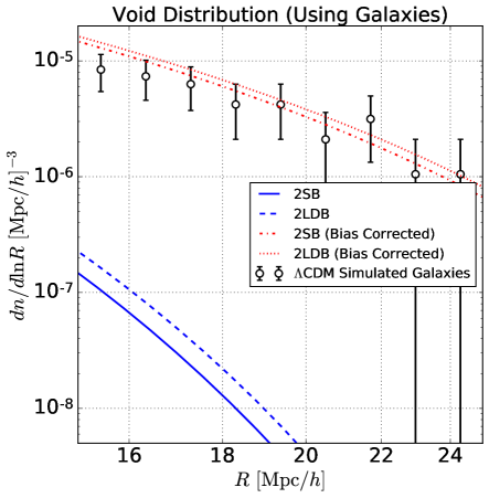
Figure 11: Void abundance distribution as a function of void radius for voids detected in the galaxy mock catalogue for $\Lambda$CDM (open circles). Also shown are the abundance predictions from the 2SB and 2LDB models with no corrections due to galaxy bias (blue solid and dashed lines respectively), as well as the same model predictions with the bias corrections (red dotted dashes and dotted lines respectively).

The main problem of our galaxy catalogues is the low number density of objects. Larger box sizes (or a galaxy population intrinsically denser) might help decrease the error bars sufficiently in order to constrain modified gravity parameters. In Fig. 12 we show the relative difference between the abundance for the three modified gravity models and GR as inferred from our simulations. We see that it is not possible to constrain the gravity model using the abundance of galaxy voids, as extracted from mock galaxy catalogues of the size considered here, due to limited statistics. Further investigations using larger or multiple boxes, or else considering a galaxy population with larger intrinsic number density should decrease Poisson errors significantly, allowing for a better investigation of void abundance in the large data sets expected for current and upcoming surveys, such as the SDSS-IV, DES, DESI, Euclid and LSST.

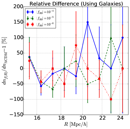
Figure 12: Relative difference in galaxy void abundance as measured in $f(R)$ gravity simulations and GR simulations. The difference is shown for $|f_{R0}|=10^{-6}$ (red squares), $10^{-5}$ (green triangles) and $10^{-6}$ (blue circles).

VI Discussion and Conclusion

We have used a suite of N-body simulations from the Isis code Llinares et al. (2014) for GR and modified gravity models to define spherical voids from underdensities detected by ZOBOV Neyrinck (2008), a void-finder based on Voronoi tesselation. We find that the void abundance in modified gravity and $\Lambda$CDM may differ by $\sim 100\%$ for the largest void radii in our simulations.

We interpreted the void abundance results through a spherical expansion model and extended Excursion Set approach. The most general theoretical model considered has two drifting diffusive barriers, with a linear dependence on the density variance (2LDB, see § III). This model depends on the theory linear power spectrum $P(k)$ and in principle has multiple parameters, namely $\delta_{c}$ and $\delta_{v}$ (the critical densities for collapse and expansion), $\beta_{c}$ and $\beta_{v}$ (the barrier slopes for halos and voids) and $D_{c}$ and $D_{v}$ (the diffusion coefficients for halos and voids). Fixing $\delta_{c}$ and $\delta_{v}$ to their GR values and under the simplifying assumption that $\beta=\beta_{c}=\beta_{v}$, the model depends on two free parameters: $\beta$ and $D=D_{c}+D_{v}$. Interestingly, our model accounts for the void-in-cloud effect and generalizes previous models for void abundance based on static barriers Jennings et al. (2013). The generalizations proposed here are similar to those made by Maggiore and Riotto (2010a, b) in the context of halos.

Since our model requires the linear power spectrum in modified gravity, we have implemented a numerical evolution of the linear perturbation equations for general theories of modified gravity parametrized by Eq. (6). We compared our computation to that from MGCAMB for $f(R)$ gravity and found very good agreement. We then use this implementation to compute the linear spectrum for both $f(R)$ and symmetron gravity.

We also considered approximate equations for spherical collapse and spherical expansion and derived the spherical collapse parameters $\delta_{c}$ and $\delta_{v}$ as a function of scale, recovering in particular the values in the strong and weak field regimes of $f(R)$ gravity – the latter corresponding to the GR solution. We then estimated the dependence of barriers $B_{c}$ and $B_{v}$ with the variance $S$ and derived values for $\beta_{c,v}$ and $\delta_{c,v}$. The values found did not however seem to correctly describe the void abundance from simulations, which may be due to the approximated equations used to study the expansion/collapse.

We also found that the variations on $P(k)$, $\beta$ and $D$ as a function of modified gravity were much stronger than those from $\delta_{c}$ and $\delta_{v}$. Therefore, in our modeling of void abundance we kept $\delta_{c}$ and $\delta_{v}$ fixed to their GR values, and took $\beta$ and $D$ as free parameters to be fit from simulations. Although beyond the scope of this work, we envision that it should be possible to derive the model parameters from first principles in the future.

By comparing the measured void abundance from the simulations to the theoretical models considered, we found the best fit values for $\beta$ and $D$ in each gravity theory and each abundance model. In particular, we found that these parameters were best-fit for models with linear diffusive barriers (see Figs. 6, 7 and Table 4), indicating that the addition of these features is important to describe modified gravity effects on void abundance. This allowed us to then fit for $\beta$ and $D$ as a function of modified gravity parameters, namely $|f_{R0}|$ in the case of $f(R)$ gravity, and $z_{SSB}$ in the case of symmetron.

Next we used these fits to check how well the calibrated models could recover the modified gravity parameters from hypothetical and idealized void abundance observations. We compared the void abundance measured in simulations to the model predictions and performed an MCMC search for the gravity parameters. Since the predictions were calibrated from the simulations themselves, our results may be highly optimistic. Nonetheless, we found that the models with linear diffusive barriers recover the modified gravity parameters better than the model with static barriers for all gravity theories (see Figs. 9, 10 and Table 5). We also found that when using voids found in the GR simulation to fit for modified gravity parameters, we seem to properly recover the GR limit at the $2\sigma$ level. Since we only used one simulation for each gravity model considered, our results have considerable uncertainties. We expect these to improve significantly with the use of multiple and larger simulations.

Finally, we populated the dark matter halos found in the simulations with galaxies in order to access the possibility of modeling the abundance of galaxy voids. For the GR case, we found that the same model with linear diffusive barriers properly describes the abundance of galaxy voids, provided we use the galaxy bias to correct for the effective overdensity $\Delta$ used for void detection. However, the error bars were too large to allow for any signal in the modified gravity case relative to GR. Again since we used a single simulation for each gravity, our results for galaxy voids are even more affected by shot noise and unknown sample variance effects.

Current and upcoming spectroscopic and photometric galaxy surveys will produce large catalogs of galaxies, clusters and voids. Observed void properties from real data are affected by nontrivial effects such as surveys masks and depth variations in the sky. One could partially characterize these effects from realistic simulations and understand their possible consequences, such as inappropriately breaking large voids into multiple smaller ones or vice-versa (i.e. merging small voids into larger ones). Assuming that such effects can be understood and characterized, we expect that the properties of voids, including their abundance, clustering properties and profiles, will be very important to constrain cosmological models, especially modified gravity. In particular, since voids and halos respond differently to screening effects present in viable modified gravity theories, a combination of voids and halo properties should be particularly effective in constraining and distinguishing alternative gravity models.

References

- Brax and Davis (2015) P. Brax and A.-C. Davis, ArXiv e-prints (2015), arXiv:1506.01519 .
- de Martino et al. (2015) I. de Martino, M. De Laurentis, and S. Capozziello, Universe 1, 123 (2015), arXiv:1507.06123 [gr-qc] .
- Brax (2012) P. Brax, ArXiv e-prints (2012), arXiv:1211.5237 [hep-th] .
- Khoury and Weltman (2004a) J. Khoury and A. Weltman, Physical Review Letters 93, 171104 (2004a), astro-ph/0309300 .
- Khoury and Weltman (2004b) J. Khoury and A. Weltman, Phys. Rev. D 69, 044026 (2004b), astro-ph/0309411 .
- Mota and Shaw (2007) D. F. Mota and D. J. Shaw, Phys. Rev. D75, 063501 (2007), arXiv:hep-ph/0608078 [hep-ph] .
- Gannouji et al. (2010) R. Gannouji, B. Moraes, D. F. Mota, D. Polarski, S. Tsujikawa, and H. A. Winther, Phys. Rev. D82, 124006 (2010), arXiv:1010.3769 [astro-ph.CO] .
- Gubser and Khoury (2004) S. S. Gubser and J. Khoury, Phys. Rev. D70, 104001 (2004), arXiv:hep-ph/0405231 [hep-ph] .
- Navarro and Van Acoleyen (2007) I. Navarro and K. Van Acoleyen, JCAP 0702, 022 (2007), arXiv:gr-qc/0611127 [gr-qc] .
- Vainshtein (1972) A. I. Vainshtein, Physics Letters B 39, 393 (1972).
- Babichev and Deffayet (2013) E. Babichev and C. Deffayet, Classical and Quantum Gravity 30, 184001 (2013), arXiv:1304.7240 [gr-qc] .
- Falck et al. (2014) B. Falck, K. Koyama, G.-b. Zhao, and B. Li, JCAP 1407, 058 (2014), arXiv:1404.2206 [astro-ph.CO] .
- Hinterbichler and Khoury (2010) K. Hinterbichler and J. Khoury, Physical Review Letters 104, 231301 (2010), arXiv:1001.4525 [hep-th] .
- Hinterbichler et al. (2011) K. Hinterbichler, J. Khoury, A. Levy, and A. Matas, Phys. Rev. D 84, 103521 (2011), arXiv:1107.2112 [astro-ph.CO] .
- Hammami and Mota (2015) A. Hammami and D. F. Mota, (2015), arXiv:1505.06803 [astro-ph.CO] .
- Davis et al. (2012) A.-C. Davis, B. Li, D. F. Mota, and H. A. Winther, Astrophys. J. 748, 61 (2012), arXiv:1108.3081 [astro-ph.CO] .
- Oyaizu (2008) H. Oyaizu, Phys. Rev. D 78, 123523 (2008), arXiv:0807.2449 .
- Oyaizu et al. (2008) H. Oyaizu, M. Lima, and W. Hu, Phys. Rev. D 78, 123524 (2008), arXiv:0807.2462 .
- Schmidt et al. (2009) F. Schmidt, M. Lima, H. Oyaizu, and W. Hu, Phys. Rev. D 79, 083518 (2009), arXiv:0812.0545 .
- Schmidt (2009a) F. Schmidt, Phys. Rev. D 80, 123003 (2009a), arXiv:0910.0235 [astro-ph.CO] .
- Schmidt (2009b) F. Schmidt, Phys. Rev. D 80, 043001 (2009b), arXiv:0905.0858 [astro-ph.CO] .
- Clifton et al. (2005) T. Clifton, D. F. Mota, and J. D. Barrow, Mon. Not. Roy. Astron. Soc. 358, 601 (2005), arXiv:gr-qc/0406001 [gr-qc] .
- Khoury and Wyman (2009) J. Khoury and M. Wyman, Phys. Rev. D 80, 064023 (2009), arXiv:0903.1292 [astro-ph.CO] .
- Li and Zhao (2009) B. Li and H. Zhao, Phys. Rev. D 80, 044027 (2009), arXiv:0906.3880 [astro-ph.CO] .
- Schmidt et al. (2010) F. Schmidt, W. Hu, and M. Lima, Phys. Rev. D 81, 063005 (2010), arXiv:0911.5178 [astro-ph.CO] .
- Ferraro et al. (2011) S. Ferraro, F. Schmidt, and W. Hu, Phys. Rev. D 83, 063503 (2011), arXiv:1011.0992 .
- Zhao et al. (2011) G.-B. Zhao, B. Li, and K. Koyama, Phys. Rev. D 83, 044007 (2011), arXiv:1011.1257 [astro-ph.CO] .
- Li and Barrow (2011) B. Li and J. D. Barrow, Phys. Rev. D 83, 024007 (2011), arXiv:1005.4231 [astro-ph.CO] .
- Li et al. (2013) B. Li, A. Barreira, C. M. Baugh, W. A. Hellwing, K. Koyama, S. Pascoli, and G.-B. Zhao, Journal of Cosmology and Astroparticle Physics 11, 012 (2013), arXiv:1308.3491 [astro-ph.CO] .
- Wyman et al. (2013) M. Wyman, E. Jennings, and M. Lima, Phys. Rev. D 88, 084029 (2013), arXiv:1303.6630 [astro-ph.CO] .
- Arnold et al. (2014) C. Arnold, E. Puchwein, and V. Springel, Mon. Not. R. Astron. Soc. 440, 833 (2014), arXiv:1311.5560 .
- Brax et al. (2013) P. Brax, A.-C. Davis, B. Li, H. A. Winther, and G.-B. Zhao, Journal of Cosmology and Astroparticle Physics 4, 029 (2013), arXiv:1303.0007 [astro-ph.CO] .
- Candlish et al. (2015) G. N. Candlish, R. Smith, and M. Fellhauer, Mon. Not. R. Astron. Soc. 446, 1060 (2015), arXiv:1410.3844 .
- Hagala et al. (2016) R. Hagala, C. Llinares, and D. F. Mota, Astron. Astrophys. 585, A37 (2016), arXiv:1504.07142 .
- Achitouv et al. (2015) I. Achitouv, M. Baldi, E. Puchwein, and J. Weller, (2015), arXiv:1511.01494 [astro-ph.CO] .
- Winther et al. (2015) H. A. Winther et al., Mon. Not. Roy. Astron. Soc. 454, 4208 (2015), arXiv:1506.06384 [astro-ph.CO] .
- Barreira et al. (2016) A. Barreira, C. Llinares, S. Bose, and B. Li, ArXiv e-prints (2016), arXiv:1601.02012 .
- Li and Hu (2011) Y. Li and W. Hu, Phys. Rev. D 84, 084033 (2011), arXiv:1107.5120 .
- Taruya et al. (2014) A. Taruya, T. Nishimichi, F. Bernardeau, T. Hiramatsu, and K. Koyama, Phys. Rev. D 90, 123515 (2014), arXiv:1408.4232 .
- Bourliot et al. (2007) F. Bourliot, P. G. Ferreira, D. F. Mota, and C. Skordis, Phys. Rev. D75, 063508 (2007), arXiv:astro-ph/0611255 [astro-ph] .
- Lombriser et al. (2013) L. Lombriser, B. Li, K. Koyama, and G.-B. Zhao, Phys. Rev. D 87, 123511 (2013), arXiv:1304.6395 [astro-ph.CO] .
- Lombriser et al. (2012) L. Lombriser, F. Schmidt, T. Baldauf, R. Mandelbaum, U. Seljak, and R. E. Smith, Phys. Rev. D 85, 102001 (2012), arXiv:1111.2020 [astro-ph.CO] .
- Koyama et al. (2009) K. Koyama, A. Taruya, and T. Hiramatsu, Phys. Rev. D 79, 123512 (2009), arXiv:0902.0618 [astro-ph.CO] .
- Brax and Valageas (2012) P. Brax and P. Valageas, Phys. Rev. D 86, 063512 (2012), arXiv:1205.6583 [astro-ph.CO] .
- Cooray and Sheth (2002) A. Cooray and R. K. Sheth, Phys. Rept. 372, 1 (2002), arXiv:astro-ph/0206508 [astro-ph] .
- Press and Schechter (1974) W. H. Press and P. Schechter, Astrophys. J. 187, 425 (1974).
- Sheth et al. (2001) R. K. Sheth, H. J. Mo, and G. Tormen, Mon. Not. R. Astron. Soc. 323, 1 (2001), astro-ph/9907024 .
- Bond et al. (1991) J. R. Bond, S. Cole, G. Efstathiou, and N. Kaiser, Astrophys. J. 379, 440 (1991).
- Tinker et al. (2008) J. Tinker, A. V. Kravtsov, A. Klypin, K. Abazajian, M. Warren, G. Yepes, S. Gottlöber, and D. E. Holz, Astrophys. J. 688, 709 (2008), arXiv:0803.2706 .
- Jenkins et al. (2001) A. Jenkins, C. S. Frenk, S. D. M. White, J. M. Colberg, S. Cole, A. E. Evrard, H. M. P. Couchman, and N. Yoshida, Mon. Not. R. Astron. Soc. 321, 372 (2001), astro-ph/0005260 .
- Lima and Hu (2005) M. Lima and W. Hu, Phys. Rev. D 72, 043006 (2005), astro-ph/0503363 .
- Clampitt et al. (2013) J. Clampitt, Y.-C. Cai, and B. Li, Mon. Not. R. Astron. Soc. 431, 749 (2013), arXiv:1212.2216 [astro-ph.CO] .
- Pisani et al. (2015) A. Pisani, P. M. Sutter, N. Hamaus, E. Alizadeh, R. Biswas, B. D. Wandelt, and C. M. Hirata, ArXiv e-prints (2015), arXiv:1503.07690 .
- Sánchez et al. (2016) C. Sánchez, J. Clampitt, A. Kovacs, B. Jain, J. García-Bellido, S. Nadathur, D. Gruen, N. Hamaus, D. Huterer, P. Vielzeuf, A. Amara, C. Bonnett, J. DeRose, W. G. Hartley, M. Jarvis, O. Lahav, R. Miquel, E. Rozo, E. S. Rykoff, E. Sheldon, R. H. Wechsler, J. Zuntz, T. M. C. Abbott, F. B. Abdalla, J. Annis, A. Benoit-Lévy, G. M. Bernstein, R. A. Bernstein, E. Bertin, D. Brooks, E. Buckley-Geer, A. Carnero Rosell, M. Carrasco Kind, J. Carretero, M. Crocce, C. E. Cunha, C. B. D’Andrea, L. N. da Costa, S. Desai, H. T. Diehl, J. P. Dietrich, P. Doel, A. E. Evrard, A. Fausti Neto, B. Flaugher, P. Fosalba, J. Frieman, E. Gaztanaga, R. A. Gruendl, G. Gutierrez, K. Honscheid, D. J. James, E. Krause, K. Kuehn, M. Lima, M. A. G. Maia, J. L. Marshall, P. Melchior, A. A. Plazas, K. Reil, A. K. Romer, E. Sanchez, M. Schubnell, I. Sevilla-Noarbe, R. C. Smith, M. Soares-Santos, F. Sobreira, E. Suchyta, G. Tarle, D. Thomas, A. R. Walker, and J. Weller, ArXiv e-prints (2016), arXiv:1605.03982 .
- Massara et al. (2015) E. Massara, F. Villaescusa-Navarro, M. Viel, and P. M. Sutter, Journal of Cosmology and Astroparticle Physics 11, 018 (2015), arXiv:1506.03088 .
- Cai et al. (2016) Y.-C. Cai, A. Taylor, J. A. Peacock, and N. Padilla, ArXiv e-prints (2016), arXiv:1603.05184 .
- Wojtak et al. (2016) R. Wojtak, D. Powell, and T. Abel, Mon. Not. R. Astron. Soc. 458, 4431 (2016), arXiv:1602.08541 .
- Pollina et al. (2016) G. Pollina, M. Baldi, F. Marulli, and L. Moscardini, Mon. Not. R. Astron. Soc. 455, 3075 (2016), arXiv:1506.08831 .
- Nadathur and Hotchkiss (2015a) S. Nadathur and S. Hotchkiss, ArXiv e-prints (2015a), arXiv:1504.06510 .
- Nadathur and Hotchkiss (2015b) S. Nadathur and S. Hotchkiss, ArXiv e-prints (2015b), arXiv:1507.00197 .
- Nadathur et al. (2014) S. Nadathur, S. Hotchkiss, J. M. Diego, I. T. Iliev, S. Gottlöber, W. A. Watson, and G. Yepes, ArXiv e-prints (2014), arXiv:1412.8372 .
- Sheth and van de Weygaert (2004) R. K. Sheth and R. van de Weygaert, Mon. Not. R. Astron. Soc. 350, 517 (2004), astro-ph/0311260 .
- Corasaniti and Achitouv (2011a) P. S. Corasaniti and I. Achitouv, Physical Review Letters 106, 241302 (2011a), arXiv:1012.3468 [astro-ph.CO] .
- Maggiore and Riotto (2010a) M. Maggiore and A. Riotto, Astrophys. J. 711, 907 (2010a), arXiv:0903.1249 [astro-ph.CO] .
- Maggiore and Riotto (2010b) M. Maggiore and A. Riotto, Astrophys. J. 717, 515 (2010b), arXiv:0903.1250 .
- Jennings et al. (2013) E. Jennings, Y. Li, and W. Hu, Mon. Not. R. Astron. Soc. 434, 2167 (2013), arXiv:1304.6087 .
- Achitouv and Corasaniti (2012) I. E. Achitouv and P. S. Corasaniti, Journal of Cosmology and Astroparticle Physics 2, 002 (2012), arXiv:1109.3196 [astro-ph.CO] .
- Zentner (2007) A. R. Zentner, International Journal of Modern Physics D 16, 763 (2007), astro-ph/0611454 .
- Pace et al. (2010) F. Pace, J.-C. Waizmann, and M. Bartelmann, Mon. Not. R. Astron. Soc. 406, 1865 (2010), arXiv:1005.0233 [astro-ph.CO] .
- Hu and Sawicki (2007) W. Hu and I. Sawicki, Phys. Rev. D 76, 064004 (2007), arXiv:0705.1158 .
- Lewis et al. (2000) A. Lewis, A. Challinor, and A. Lasenby, Astrophys. J. 538, 473 (2000), astro-ph/9911177 .
- Hojjati et al. (2011) A. Hojjati, L. Pogosian, and G.-B. Zhao, Journal of Cosmology and Astroparticle Physics 8, 005 (2011), arXiv:1106.4543 [astro-ph.CO] .
- Zhao et al. (2009) G.-B. Zhao, L. Pogosian, A. Silvestri, and J. Zylberberg, Phys. Rev. D 79, 083513 (2009), arXiv:0809.3791 .
- Kopp et al. (2013) M. Kopp, S. A. Appleby, I. Achitouv, and J. Weller, Phys. Rev. D 88, 084015 (2013), arXiv:1306.3233 [astro-ph.CO] .
- Borisov et al. (2012) A. Borisov, B. Jain, and P. Zhang, Phys. Rev. D 85, 063518 (2012), arXiv:1102.4839 .
- Corasaniti and Achitouv (2011b) P. S. Corasaniti and I. Achitouv, Physical Review Letters 106, 241302 (2011b), arXiv:1012.3468 [astro-ph.CO] .
- Llinares et al. (2014) C. Llinares, D. F. Mota, and H. A. Winther, Astron. Astrophys. 562, A78 (2014), arXiv:1307.6748 .
- Neyrinck (2008) M. C. Neyrinck, Mon. Not. R. Astron. Soc. 386, 2101 (2008), arXiv:0712.3049 .
- Foreman-Mackey et al. (2013) D. Foreman-Mackey, D. W. Hogg, D. Lang, and J. Goodman, Pub. Astron. Soc. Pacific 125, 306 (2013), arXiv:1202.3665 [astro-ph.IM] .
- Planck Collaboration et al. (2015) Planck Collaboration, P. A. R. Ade, N. Aghanim, M. Arnaud, M. Ashdown, J. Aumont, C. Baccigalupi, A. J. Banday, R. B. Barreiro, J. G. Bartlett, and et al., ArXiv e-prints (2015), arXiv:1502.01589 .
- Zheng et al. (2007) Z. Zheng, A. L. Coil, and I. Zehavi, Astrophys. J. 667, 760 (2007), astro-ph/0703457 .
- Sutter et al. (2015) P. M. Sutter, G. Lavaux, N. Hamaus, A. Pisani, B. D. Wandelt, M. Warren, F. Villaescusa-Navarro, P. Zivick, Q. Mao, and B. B. Thompson, Astronomy and Computing 9, 1 (2015), arXiv:1406.1191 .
- Navarro et al. (1996) J. F. Navarro, C. S. Frenk, and S. D. M. White, Astrophys. J. 462, 563 (1996), arXiv:astro-ph/9508025 [astro-ph] .