Importance sampling type estimators based on approximate marginal MCMC

Abstract.

We consider importance sampling (IS) type weighted estimators based on Markov chain Monte Carlo (MCMC) targeting an approximate marginal of the target distribution. In the context of Bayesian latent variable models, the MCMC typically operates on the hyperparameters, and the subsequent weighting may be based on IS or sequential Monte Carlo (SMC), but allows for multilevel techniques as well. The IS approach provides a natural alternative to delayed acceptance (DA) pseudo-marginal/particle MCMC, and has many advantages over DA, including a straightforward parallelisation and additional flexibility in MCMC implementation. We detail minimal conditions which ensure strong consistency of the suggested estimators, and provide central limit theorems with expressions for asymptotic variances. We demonstrate how our method can make use of SMC in the state space models context, using Laplace approximations and time-discretised diffusions. Our experimental results are promising and show that the IS type approach can provide substantial gains relative to an analogous DA scheme, and is often competitive even without parallelisation.

1. Introduction

Markov chain Monte Carlo (MCMC) has become a standard tool in Bayesian analysis. The greatest benefit of MCMC is its general applicability — it is guaranteed to be consistent with virtually no assumptions on the underlying model. However, the practical applicability of MCMC generally depends on the dimension of the unknown variables, the number of data, and the computational resources available. Because MCMC is only asymptotically unbiased, and sequential in nature, it can be difficult to implement efficiently with modern parallel and distributed computing facilities [64, 45, 104].

We promote a simple two-phase inference approach, based on importance sampling (IS), which is well-suited for parallel implementation. It combines a typically low-dimensional MCMC targeting an approximate marginal distribution with independently calculated estimators, which yield exact inference over the full posterior. The estimator is similar to self-normalised importance sampling, but is more general, allowing for sequential Monte Carlo and multilevel type corrections. The method is naturally applicable in a latent variable models context, where the MCMC operates on the hyperparameter distribution using an approximate marginal likelihood, and re-weighting is based on a sampling scheme on the latent variables. We detail the application of the method with Bayesian state space models, where we use importance sampling and particle filters for correction.

1.1. Related work

We consider a framework which combines and generalises upon various previously suggested methods, which, to our knowledge, has not been systematically explored before. Importance sampling correction of MCMC has been suggested early in the MCMC literature [e.g. 47, 39, 20], and used, for instance, to estimate Bayes factors using a single MCMC output [21]. Related confidence intervals have been suggested based on regeneration [11] and in case of multiple Markov chains [95]. Using unbiased estimators of importance weights in this context has been suggested at least in [65, 68], who consider marginal inference with a generalisation of the pseudo-marginal method, allowing for likelihood estimators that may take negative values, and in [82] with data sub-sampling.

Nested or compound sampling has also appeared in many forms in the Monte Carlo literature. The SMC² algorithm [13] is based on an application of nested sequential Monte Carlo steps, which has similarities with our framework, and the IS² method [97] focuses on the case where the preliminary inference is based on independent sampling. We focus on the MCMC approximation of the marginal distribution, which we believe often to be easily implementable in practice, also when the marginal distribution has a non-standard form. The Markov dependence in the marginal Monte Carlo approximation comes with some extra theoretical issues, which we address in detail.

Our setting highlights explicitly the connection of IS type correction and delayed acceptance (DA) [34, 67, 15], and recently developed pseudo-marginal type MCMC [4, 65] such as particle MCMC [2], grouped independence Metropolis-Hastings [9], approximate Bayesian computation (ABC) MCMC [69], the algorithm for estimation of discretely observed diffusions suggested in [10], and annealed IS [58, 74]. Theoretical advances of pseudo-marginal methods [6, 7, 28, 92, 3, 14, 66] have already led to more efficient implementation of such methods, but have also revealed fundamental limitations. For instance, the methods may suffer from slow (non-geometric) convergence in practically interesting scenarios [4, 63]. Adding dependence to the estimators [cf. 7], such as using the recently proposed correlated version of the pseudo-marginal MCMC [18], may help in more efficient implementation in certain scenarios, but a successful implementation of such a method may not always be possible, and the question of efficient parallelisability remains a challenge. The blocked parallelisable particle Gibbs [93] has appealing limiting properties, but its implementation still requires synchronisation between every update cycle, which may be costly in some computing environments.

The IS approach which we propose may assuage some of the aforementioned challenges of the pseudo-marginal framework, by replacing a pseudo-marginal MCMC with a fast-mixing but approximate MCMC, and postponing the computationally intensive calculations to parallelisable post-processing; see Section 2.3.

1.2. Outline

We introduce a generic Bayesian latent variable model in Section 2, detail our approach algorithmically, and compare it with DA. We also discuss practical implications, modifications and possible extensions. After introducing notation in Section 3, we formulate general IS type correction of MCMC and related consistency results in Section 4. We detail the general case (Theorem 3), based on a concept (Definition 2), which we call a ‘proper weighting’ scheme (following the terminology of Liu [67]), which is natural and convenient in many contexts. In Section 5, we state central limit theorems and expressions for asymptotic variances. Section 6 focuses on estimators which calculate IS correction once for each accepted state, stemming from a so-called ‘jump chain’ representation. Section 7 details consistency of our estimators in case the approximate chain is pseudo-marginal.

We then focus on state-space models with linear-Gaussian state dynamics in Section 8, and show how a Laplace approximation can be used both for approximate inference, and for construction of efficient proper weighting schemes. Section 9 describes an instance of our approach in the context of discretely observed diffusions, with an approximate pseudo-marginal chain. We compare empirically several algorithmic variations in Section 10 with Poisson observations, with a stochastic volatility model and with a discretely observed geometric Brownian motion. Section 11 concludes, with discussion.

2. The proposed latent variable model inference methodology

A generic Bayesian latent variable model is defined in terms of three random vector, and corresponding conditional densities:

• $\Theta\sim\mathrm{pr}(\,\cdot\,)$ — prior density of (hyper)parameters,

• $X\mid\Theta=\theta\sim\mu^{(\theta)}(\,\cdot\,)$ — prior of latent variables given parameters, and

• $Y\mid(\Theta=\theta,X=x)\sim g^{(\theta)}(\,\cdot\,\mid x)$ — the observation model.

The aim is inference over the posterior of $(\Theta,X)$ given observations $Y=y$, with density $\pi(\theta,x)\propto\mathrm{pr}(\theta)\mu^{(\theta)}(x)g^{(\theta)}(y\mid x)$. Standard MCMC algorithms may, in principle, be applied directly for inference, but the typical high dimension of the latent variable $x$ and the common strong dependency structures often lead to poor performance of generic algorithms.

Our inference approach focuses on the specific structure of the model, based on the factorisation $\pi(\theta,x)=\pi_{m}(\theta)r(x\mid\theta)$, where the marginal posterior density $\pi_{m}$ and the corresponding conditional $r$ are:

$$\pi_{m}(\theta)\mathrel{\mathop{:}}=\int\pi(\theta,x)\mathrm{d}x\propto\mathrm{pr}(\theta)L(\theta)\qquad\text{and}\qquad r(x\mid\theta)\mathrel{\mathop{:}}=\frac{p^{(\theta)}(x,y)}{L(\theta)},$$

with the joint density of the latent and the observed $p^{(\theta)}(x,y)$, and the marginal likelihood $L(\theta)$ given as follows:

$$p^{(\theta)}(x,y) \mathrel{\mathop{:}}=\mu^{(\theta)}(x)g^{(\theta)}(y\mid x) L(\theta) \mathrel{\mathop{:}}=\int p^{(\theta)}(x,y)\mathrm{d}x.$$ and

Two particularly successful latent variable model inference methods, the integrated nested Laplace approximation (INLA) [87] and the particle MCMC methods (PMCMC) [2], rely on this structure. In essence, the INLA is based on an efficient Laplace approximation $p_{a}^{(\theta)}(x,y)$ of $p^{(\theta)}(x,y)$, determining an approximate marginal likelihood $L_{a}(\theta)$ and approximate conditional distribution $r_{a}(x\mid y)$. Particle MCMC uses a specialised SMC algorithm, which provides an unbiased approximation of expectations with respect to $p^{(\theta)}(x,y)$ allowing for exact inference, and which is particularly efficient in the state space models context.

2.1. An algorithmic description

The primary aim of this paper is the efficient use of an approximate marginal likelihood $L_{a}(\theta)$ within a Monte Carlo framework that leads to efficient, parallelisable and exact inference. For instance, Laplace approximations often lead to a natural choice for $L_{a}(\theta)$. The inference method which we propose comprises two algorithmic phases, which are summarised below:

1. Simulate a Markov chain $(\Theta_{k})_{k=1,\ldots,n}$ targeting an approximate hyperparameter posterior $\pi_{a}(\theta)\propto\mathrm{pr}(\theta)L_{a}(\theta).$

2. For each $\Theta_{k}$, sample $(V_{k}^{(i)},X_{k}^{(i)})_{i=1,\ldots,m}$ where $V_{k}^{(i)}\in\mathbb{R}$ and $X_{k}^{(i)}$ are in the latent variable space, and calculate $W_{k}^{(i)}\mathrel{\mathop{:}}=V_{k}^{(i)}/L_{a}(\Theta_{k})$, which determine a weighted estimator

   (1) $$E_{n}(f)\mathrel{\mathop{:}}=\frac{\sum_{k=1}^{n}\sum_{i=1}^{m}W_{k}^{(i)}f(\Theta_{k},X_{k}^{(i)})}{\sum_{j=1}^{n}\sum_{\ell=1}^{m}W_{j}^{(\ell)}}$$

   of the full posterior expectation $\mathbb{E}_{\pi}[f(\Theta,X)]=\int f(\theta,x)\pi(\theta,x)\mathrm{d}\theta\mathrm{d}x$.

The following conditions are essential to ensure the consistency of the estimator:

1. The approximation is consistent, in the sense that $L_{a}(\theta)>0$ whenever $L(\theta)>0$, and $\int\mathrm{pr}(\theta)L_{a}(\theta)\mathrm{d}\theta<\infty$.

2. The Markov chain $(\Theta_{k})_{k\geq n}$ is Harris ergodic (Definition 1) with respect to $\pi_{a}$.

3. Denoting $f^{*}(\theta)\mathrel{\mathop{:}}=\mathbb{E}_{\pi}[f(\Theta,X)\mid\Theta=\theta]=\int r(x\mid\theta)f(\theta,x)\mathrm{d}x$, there exists a constant $c_{w}>0$ such that

   (2) $$\mathbb{E}\bigg{[}\sum_{i=1}^{m}V_{k}^{(i)}f(\Theta_{k},X_{k}^{(i)})\mathrel{\bigg{|}}\Theta_{k}=\theta\bigg{]} =c_{w}L(\theta)f^{*}(\theta),$$

   for all $\theta\in\mathsf{T}$, all functions $f$ of interest, and for $f\equiv 1$ (i.e. (2) holds with $f(\,\cdot\,)$ and $f^{*}(\,\cdot\,)$ omitted). The value of $c_{w}$ need not be known.

Both C1 and C2 are easily satisfied by construction of the approximation, and C3 is satisfied by many schemes. Appendix D reviews how the particle filter leads to such schemes. The conditions C1–C3 are key, but unfortunately not enough to guarantee consistency, which requires also a (mild) integrability condition, which $(W_{k}^{(i)},X_{k}^{(i)})_{k=1,\ldots,n;\,i=1,\ldots,m}$ must satisfy. Fortunately, in the common case of non-negative $V_{k}^{(i)}$, this integrability is guaranteed if also $|f|$ satisfies (2); see Section 4 for details. Further conditions ensure a central limit theorem $\sqrt{n}\{E_{n}(f)-\mathbb{E}_{\pi}[f(\Theta,X)]\}\to N(0,\sigma^{2})$, as detailed in Section 5.

When Phase 1 is a Metropolis-Hastings algorithm, it is possible to generate only one batch of $(\tilde{V}_{k}^{(i)},\tilde{X}_{k}^{(i)})_{i=1,\ldots,m}$ for each accepted state $(\tilde{\Theta}_{k})$. If $N_{k}$ stands for the time spent at $\tilde{\Theta}_{k}$, then the corresponding weights are determined as $\tilde{W}_{k}\mathrel{\mathop{:}}=N_{k}V_{k}^{(i)}/L_{a}(\tilde{\Theta}_{k})$; see Section 6 for details about such ‘jump chain’ estimators.

2.2. Use with approximate pseudo-marginal MCMC

In many scenarios, such as with time-discretised diffusions, the latent variable prior density $\mu^{(\theta)}$ cannot be evaluated, and exact simulation is impossible or very expensive. Simulation is also expensive with a fine enough time-discretisation.

A coarsely discretised model leads to a natural cheap approximation $\hat{\mu}^{(\theta)}$, but in Phase 1, the Markov chain will often be a pseudo-marginal MCMC [cf. 4], in which case our scheme would have the following form:

1. Simulate a pseudo-marginal Metropolis-Hastings chain $(\Theta_{k},U_{k})$ for $k=1,\ldots,n$, following

   1. Draw a proposal $\tilde{\Theta}_{k}$ from $q(\Theta_{k-1},\,\cdot\,)$ and given $\tilde{\Theta}_{k}$, construct an estimator $\tilde{U}_{k}\geq 0$ such that $\mathbb{E}[\tilde{U}_{k}\mid\tilde{\Theta}_{k}=\theta]=L_{a}(\theta)$.

   2. With probability $\min\Big{\{}1,\frac{\mathrm{pr}(\tilde{\Theta}_{k})\tilde{U}_{k}q(\tilde{\Theta}_{k},\Theta_{k-1})}{\mathrm{pr}(\Theta_{k-1})U_{k-1}q(\Theta_{k-1},\tilde{\Theta}_{k})}\Big{\}}$, accept and set $(\Theta_{k},U_{k})=(\tilde{\Theta}_{k},\tilde{U}_{k})$; otherwise reject the move.

2. For each $(\Theta_{k},U_{k})$, sample $(V_{k}^{(i)},X_{k}^{(i)})_{i=1,\ldots,m}$ and set $W_{k}^{(i)}\mathrel{\mathop{:}}=V_{k}^{(i)}/U_{k}$, which determine the estimator as in (1).

Algorithmically, the pseudo-marginal version above is similar to the method in Section 2.1, with the likelihood $L_{a}(\Theta_{k})$ replaced with its estimator $U_{k}$. The requirements for the approximate likelihood C1 and its estimator C3 remain identical, and C2 must hold for the pseudo-marginal chain $(\Theta_{k},U_{k})_{k\geq 1}$, together with the following condition:

1. The estimators $\tilde{U}_{k}$ are strictly positive, almost surely, for all $\tilde{\Theta}_{k}\in\mathsf{T}$.

These are enough to guarantee consistency; see Section 7, and in particular Proposition 17 for details, which also justifies why C4 is needed for consistency. In practice it may be easily satisfied, because the likelihood estimators $\tilde{U}_{k}$ may be inflated, if necessary (see Section 11).

Note that the variables $(V_{k}^{(i)},X_{k}^{(i)})_{i=1,\ldots,m}$ may depend on both $\Theta_{k}$ and the related likelihood estimate $U_{k}$. The dependency may be useful, if positively correlated $V_{k}^{(i)}$ and $U_{k}$ are available, leading to lower variance weights $W_{k}^{(i)}=V_{k}^{(i)}/U_{k}$. This is similar to the correlated pseudo-marginal algorithm [18], which relies on a particular form of $V_{k}^{(i)}$ and $U_{k}$. If positively correlated structure is unavailable, $(V_{k}^{(i)},X_{k}^{(i)})_{i=1,\ldots,m}$ may be constructed independently of $U_{k}$.

2.3. Comparison with delayed acceptance

The key condition, under which we believe our method to be useful, is that the Phase 1 Markov chain is computationally relatively cheap compared to construction of the random variables $(W_{k}^{(i)},X_{k}^{(i)})$ computed in Phase 2. Similar rationale, and similar building blocks — a $\pi_{a}$-reversible Markov chain and random variables analogous to $(W_{k}^{(i)},X_{k}^{(i)})$ — have been suggested earlier for construction of a delayed acceptance (DA) pseudo-marginal MCMC scheme [cf. 43]. Such an algorithm defines a Markov chain $(\Theta_{k},W_{k}^{(i)},X_{k}^{(i)})_{k\geq 1}$, with one iteration consisting of the following steps:

1. Draw $\tilde{\Theta}_{k}\sim P(\Theta_{k-1},\,\cdot\,)$. If $\tilde{\Theta}_{k}=\Theta_{k-1}$ reject and set $(\Theta_{k},W_{k}^{(i)},X_{k}^{(i)})=(\Theta_{k-1},W_{k-1}^{(i)},X_{k-1}^{(i)})$; otherwise go to (DA 2).

2. Conditional on $\tilde{\Theta}_{k}$, draw $(\tilde{V}_{k}^{(i)},\tilde{X}_{k}^{(i)})_{i=1,\ldots,m}$ which satisfy (2) with $\tilde{\Theta}_{k}$ in place of $\Theta_{k}$, and set $\tilde{W}_{k}^{(i)}\mathrel{\mathop{:}}=\tilde{V}_{k}^{(i)}/L_{a}(\tilde{\Theta}_{k})$. With probability $\min\Big{\{}1,\frac{\sum_{i=1}^{m}\tilde{W}_{k}^{(i)}}{\sum_{\ell=1}^{m}W_{k-1}^{(\ell)}}\Big{\}}$, accept and set $(\Theta_{k},W_{k}^{(i)},X_{k}^{(i)})=(\tilde{\Theta}_{k},\tilde{W}_{k}^{(i)},\tilde{X}_{k}^{(i)})$; otherwise reject and set $(\Theta_{k},W_{k}^{(i)},X_{k}^{(i)})=(\Theta_{k-1},W_{k-1}^{(i)},X_{k-1}^{(i)})$

If the pseudo-marginal method is used in DA 1 the value $L_{a}(\Theta_{k})$ is replaced with the related likelihood estimator. Under the same assumptions as required by our scheme, and additionally requiring that $\tilde{W}_{k}^{(i)}\geq 0$, and that the Markov chain $(\Theta_{k},W_{k}^{(i)},X_{k}^{(i)})_{k\geq 1}$ is Harris, the DA scheme leads to a consistent estimator:

$$\frac{1}{n}\sum_{k=1}^{n}\sum_{i=1}^{m}\bigg{(}\frac{W_{k}^{(i)}}{\sum_{\ell=1}^{m}W_{k}^{(\ell)}}\bigg{)}f(\Theta_{k},X_{k}^{(i)})\xrightarrow{n\to\infty}\mathbb{E}_{\pi}[f(\Theta,X)].$$

Our IS scheme is a natural alternative to such a DA scheme, replacing the independent Metropolis-Hastings type accept-reject step DA 2 with analogous weighting. This relatively small algorithmic change brings many, potentially substantial, benefits over DA, which we note next.

1. Phase 2 corrections are entirely independent ‘post-processing’ of Phase 1 MCMC output $(\Theta_{k})_{k=1,\ldots,n}$, which is easy to implement efficiently using parallel or distributed computing. This is unlike DA 1 and DA 2, which must be iterated sequentially.

2. If Phase 2 correction variables are calculated only once for each accepted $\Theta_{k}$ (so-called ‘jump chain’ representation, see Section 6), the IS method will typically be computationally less expensive than DA with the same number of iterations, even without parallelisation.

3. The Phase 1 MCMC chain $(\Theta_{k})$ may be (further) thinned before applying (much more computationally demanding) Phase 2. Thinning of the DA chain is less likely beneficial [cf. 78].

4. In case the approximate marginal MCMC $(\Theta_{k})$ is based on a deterministic likelihood approximation, it is generally ‘safer’ than (pseudo-marginal) DA using likelihood estimators, because pseudo-marginal MCMC may have issues with mixing [cf. 6]. It is also easier to implement efficiently. For instance, popular adaptive MCMC methods which rely on acceptance rate optimisation [5, and references therein] are directly applicable.

5. Reversibility of the MCMC kernel $P$ in DA 1 is necessary, but not required for the Phase 1 MCMC.

6. The average of the weights, $n^{-1}\sum_{k=1}^{n}\sum_{i=1}^{m}W_{k}^{(i)}$, provides a consistent estimator of the ratio of the normalising constants of $\pi$ and $\pi_{a}$, which may be useful in some contexts.

7. Non-negativity of $W_{k}^{(i)}$ is required in DA 2, but not in Phase 2. This may be useful in certain contexts, where multilevel [48, 38] or debiasing [71, 84, 99] are applicable. (See also the discussion in [53] why pseudo-marginal method may not be applicable at all in such a context.)

8. The separation of ‘approximate’ Phase 1 and ‘exact’ Phase 2 allows for two-level inference. In statistical practice, preliminary analysis could be based on (fast) purely approximate inference, and the (computationally demanding) exact method could be applied only as a final verification to ensure that the approximation did not affect the findings.

To elaborate the last point, the approximate likelihood $L_{a}(\theta)$ is usually based on an approximation $p_{a}^{(\theta)}(x,y)$ of the latent model $p^{(\theta)}(x,y)$. If the approximate model admits tractable expectations of functions $f$ of interest or exact simulation, direct approximate inference is possible, because

$$\frac{1}{n}\sum_{k=1}^{n}f_{a}^{*}(\Theta_{k})\to\mathbb{E}_{\tilde{\pi}}[f(\Theta,X)],\qquad\text{where}\qquad f_{a}^{*}(\theta)\mathrel{\mathop{:}}=\mathbb{E}_{\tilde{\pi}}[f(\Theta,X)\mid\Theta=\theta],$$

with approximate joint posterior $\tilde{\pi}(\theta,x)\propto\mathrm{pr}(\theta)p_{a}^{(\theta)}(x,y)$. Then, Phase 2 allows for quantification of the bias $\mathbb{E}_{\tilde{\pi}}[f(\Theta,X)]-\mathbb{E}_{\pi}[f(\Theta,X)]$, and confirmation that both inferences lead to the same conclusions.

Even though IS is likely to bring benefits over DA in many scenarios, there are some situations where DA might perform better. In fact, DA may be used in some scenarios where IS cannot be used at all; namely, $P$ may only be reversible with respect to a positive measure that is not a probability measure, and DA can still be valid. DA may also be more robust with respect to tail behaviour of $\pi_{a}$, where IS needs more care; see the discussion in Section 11. The further theoretical work [36] provides upper bounds for ratios of the asymptotic variances of IS and DA in terms of (lower or upper) bounds of the weights $W_{k}^{(i)}$, and includes examples where DA outperforms IS and vice versa.

3. Notation and preliminaries

Throughout the paper, we consider general state spaces while using standard integral notation. If the model at hand is given in terms of standard probability densities, the rest of this paragraph can be skipped. Each space $\mathsf{X}$ is assumed to be equipped with a $\sigma$-finite dominating measure ‘$\mathrm{d}x$’ on a $\sigma$-algebra denoted with a corresponding calligraphic letter, such as $\mathcal{X}$. Product spaces are equipped with the related product $\sigma$-algebras and product dominating measures. If $\mathsf{X}$ is a subset of an Euclidean space $\mathbb{R}^{d}$, $\mathrm{d}x$ is taken by default as the Lebesgue measure and $\mathcal{X}$ as the Borel subsets of $\mathsf{X}$. $\mathbb{R}_{+}$ stands for the non-negative real numbers, and constant unit function is denoted by $\mathbf{1}$.

If $\nu$ is a probability density on $\mathsf{X}$, we define the support of $\nu$ as $\mathop{\mathrm{supp}}(\nu)\mathrel{\mathop{:}}=\{x\in\mathsf{X}\,:\,\nu(x)>0\}$, and the probability measure corresponding to $\nu$ with the same symbol $\nu(\mathrm{d}x)\mathrel{\mathop{:}}=\nu(x)\mathrm{d}x$. If $g:\mathsf{X}\to\mathbb{R}$, we denote $\nu(g)\mathrel{\mathop{:}}=\int g(x)\nu(\mathrm{d}x)$, whenever well-defined. For a probability density or measure $\nu$ on $\mathsf{X}$ and $p\in[1,\infty)$, we denote by $L^{p}(\nu)$ the set of measurable $g:\mathsf{X}\to\mathbb{R}$ with $\nu(|g|^{p})<\infty$, and by $L_{0}^{p}(\nu)\mathrel{\mathop{:}}=\{g\in L^{p}(\nu)\,:\,\nu(g)=0\}$ the corresponding set of zero-mean functions. If $P$ is a Markov transition probability, we denote the probability measure $(\nu P)(A)\mathrel{\mathop{:}}=\int\nu(\mathrm{d}x)P(x,A)$, and the function $(Pg)(x)\mathrel{\mathop{:}}=\int P(x,\mathrm{d}y)g(y)$. Iterates of transition probabilities are defined recursively through $P^{n}(x,A)\mathrel{\mathop{:}}=\int P(x,\mathrm{d}y)P^{n-1}(y,A)$ for $n\geq 1$, where $P^{0}(y,A)\mathrel{\mathop{:}}=\mathbb{I}\left(y\in A\right)$.

We follow the conventions $0/0\mathrel{\mathop{:}}=0$ and $\mathbb{N}\mathrel{\mathop{:}}=\{1,2,\ldots\}$. For integers $a\leq b$, we denote by $a{:}b$ the integers within the interval $[a,b]$. We use this notation in indexing, so that $x_{a:b}=(x_{a},\ldots,x_{b})$, $x^{(a:b)}=(x^{(a)},\ldots,x^{(b)})$. If $a>b$, then $x_{a:b}$ or $x^{(a:b)}$ is void, so that for example $g(x,y_{1:0})$ is interpreted as $g(x)$. Similarly, if $i_{1:T}$ is a vector, then $x^{(i_{1:T})}=(x^{(i_{1})},\ldots,x^{(i_{T})})$ and $x_{1:T}^{(i_{1:T})}=(x_{1}^{(i_{1})},\ldots,x_{T}^{(i_{T})})$. We also use double-indexing, such as $x_{k}^{(1:m,1:n)}=(x_{k}^{(1,1)}$, $\!\ldots\,$, $x_{k}^{(1,n)}$, $x_{k}^{(2,1)}$, $\!\ldots\,$, $x_{k}^{(m,n)})$.

Throughout the paper, we assume the underlying MCMC scheme to satisfy the following standard condition.

Definition 1 (Harris ergodicity).

A Markov chain is called Harris ergodic with respect to $\nu$, if it is $\psi$-irreducible, Harris recurrent and with invariant probability $\nu$.

Virtually all MCMC schemes are Harris ergodic [cf. 96, 75], although in some cases careless implementation could lead to a non-Harris chain [cf. 85]. Thanks to the Harris assumption, all the limit theorems which we give hold for any initial distribution of the related Markov chain.

4. General importance sampling type correction of MCMC

Hereafter, $\pi_{a}$ is a probability density on $\mathsf{T}$ and represents an approximation of a probability density $\pi_{m}$ of interest. The consistency of IS type correction relies on the following mild assumption.

Assumption 1.

The Markov chain $(\Theta_{k})_{k\geq 1}$ and the density $\pi_{a}$ satisfy:

1. $(\Theta_{k})_{k\geq 1}$ is Harris ergodic with respect to $\pi_{a}$.

2. $\mathop{\mathrm{supp}}(\pi_{m})\subset\mathop{\mathrm{supp}}(\pi_{a})$.

3. $w_{u}(\theta)\mathrel{\mathop{:}}=c_{w}\pi_{m}(\theta)/\pi_{a}(\theta)$, where $c_{w}>0$ is a constant.

If Assumption 1 holds and it is possible to calculate the unnormalised importance weight $w_{u}(\theta)$ pointwise, the chain $(\Theta_{k})_{k\geq 1}$ can be weighted in order to approximate $\pi_{m}(g)$ for every $g\in L^{1}(\pi_{m})$, using (self-normalised) importance sampling [e.g. 39, 20]

$$\frac{\sum_{k=1}^{n}w_{u}(\Theta_{k})g(\Theta_{k})}{\sum_{j=1}^{n}w_{u}(\Theta_{j})}=\frac{n^{-1}\sum_{k=1}^{n}w_{u}(\Theta_{k})g(\Theta_{k})}{n^{-1}\sum_{j=1}^{n}w_{u}(\Theta_{j})}\xrightarrow{n\to\infty}\frac{\pi_{a}(w_{u}g)}{\pi_{a}(w_{u})}=\pi_{m}(g)\qquad\text{almost surely},$$

as Harris ergodicity guarantees the almost sure convergence of both the numerator and the denominator.

In case $\pi_{m}$ is a marginal density, which we will focus on, both the ratio $w_{u}(\theta)$ and the function $g$ (which will be a conditional expectation) are typically intractable. Instead, it is often possible to construct unbiased estimators, which may be used in order to estimate the numerator and the denominator, in place of $w_{u}(\Theta_{k})$ and $g(\Theta_{k})$, under mild conditions. In order to formalise such a setting, we give the following generic condition for ratio estimators, which resemble the IS correction above.

Assumption 2.

Suppose Assumption 1 holds, and let $(S_{k})_{k\geq 1}$, where $S_{k}=\big{(}A_{k},B_{k}\big{)}\in\mathbb{R}^{2}$, be conditionally independent given $(\Theta_{k})_{k\geq 1}$, such that the distribution of $S_{k}$ depends only on the value of $\Theta_{k}$, and

1. $f_{A}(\theta)\mathrel{\mathop{:}}=\mathbb{E}[A_{k}\mid\Theta_{k}=\theta]$ satisfies $\pi_{a}(f_{A})=c_{w}\pi_{m}(g)$,

2. $f_{B}(\theta)\mathrel{\mathop{:}}=\mathbb{E}[B_{k}\mid\Theta_{k}=\theta]$ satisfies $\pi_{a}(f_{B})=c_{w}$, and

3. $\pi_{a}(m^{(1)})<\infty$ where $m^{(1)}(\theta)\mathrel{\mathop{:}}=\mathbb{E}\big{[}|A_{k}|+|B_{k}|\mathrel{\big{|}}\Theta_{k}=\theta\big{]}$.

We record the following simple statement which guarantees consistency under Assumption 2.

Lemma 1.

If Assumption 2 holds for some $g\in L^{1}(\pi_{m})$, then

$$E_{n}(g)\mathrel{\mathop{:}}=\frac{\sum_{k=1}^{n}A_{k}}{\sum_{j=1}^{n}B_{j}}\xrightarrow{n\to\infty}\pi_{m}(g)\qquad\text{almost surely}.$$

The proof of Lemma 1 follows by observing that $(\Theta_{k},S_{k})_{k\geq 1}$ is Harris ergodic, where $S_{k}=(A_{k},B_{k})$, and the functions $h_{1}(\theta,a,b)=a$ and $h_{2}(\theta,a,b)=b$ are integrable with respect to its invariant distribution $\check{\pi}(\mathrm{d}\theta\times\mathrm{d}s)\mathrel{\mathop{:}}=\pi_{a}(\mathrm{d}\theta)Q(\theta,\mathrm{d}s)$, where $Q(\theta,A)\mathrel{\mathop{:}}=\mathbb{P}(S_{k}\in A\mid\Theta_{k}=\theta)$; see Lemma 21 in Appendix A.

In the latent variable model discussed in Section 2, the aim is inference over a joint target density $\pi(\theta,x)\mathrel{\mathop{:}}=\pi_{m}(\theta)r(x\mid\theta)$ on an extended state space $\mathsf{T}\times\mathsf{X}$. For every function $f\in L^{1}(\pi)$, we denote by $f^{*}(\theta)\mathrel{\mathop{:}}=\int r(x\mid\theta)f(\theta,x)\mathrm{d}x$ the conditional expectation of $f$ given $\theta$, so $\pi(f)=\pi_{m}(f^{*})$. The following formalises a scheme which satisfies Assumption 2 with $g=f^{*}$ and therefore guarantees consistency for a class of functions $f\in\mathcal{L}\subset L^{1}(\pi)$.

Definition 2 ($\mathcal{L}$-Proper weighting scheme).

Suppose Assumption 1 holds, and let $(P_{k})_{k\geq 1}$ be conditionally independent given $(\Theta_{k})_{k\geq 1}$, such that the distribution of each $P_{k}=(M_{k},W_{k}^{(1:M_{k})},X_{k}^{(1:M_{k})})$ depends only on the value of $\Theta_{k}$, where $M_{k}\in\mathbb{N}$, $W_{k}^{(i)}\in\mathbb{R}$ and $X_{k}^{(i)}\in\mathsf{X}$. Define for any $f\in L^{1}(\pi)$,

$$\xi_{k}(f)\mathrel{\mathop{:}}=\sum_{i=1}^{M_{k}}W_{k}^{(i)}f(\Theta_{k},X_{k}^{(i)}).$$

Let $\mathcal{L}\subset L^{1}(\pi)$ be all the functions for which

1. $\mu_{f}(\theta)\mathrel{\mathop{:}}=\mathbb{E}[\xi_{k}(f)\mid\Theta_{k}=\theta]$ satisfies $\pi_{a}(\mu_{f})=c_{w}\pi(f)$, and

2. $\pi_{a}(m_{f}^{(1)})<\infty$ where $m_{f}^{(1)}(\theta)\mathrel{\mathop{:}}=\mathbb{E}\big{[}|\xi_{k}(f)|\mathrel{\big{|}}\Theta_{k}=\theta\big{]}$.

If $\mathbf{1}\in\mathcal{L}$, then $(W_{k}^{(1:M_{k})},X_{k}^{(1:M_{k})})_{k\geq 1}$ or equivalently $(\xi_{k})_{k\geq 1}$, form a $\mathcal{L}$-proper weighting scheme.

Remark 2.

Regarding Definition 2:

1. In case of non-negative weights, that is, $W_{k}^{(i)}\geq 0$ almost surely, we have $|\xi_{k}(\mathbf{1})|=\xi_{k}(\mathbf{1})$, so $f\equiv\mathbf{1}\in\mathcal{L}$ if and only if (i) holds for $f\equiv\mathbf{1}$. Further, if (i) holds for both $f$ and $|f|$, then (ii) holds, because $|\xi_{k}(f)|\leq\xi_{k}(|f|)$.

2. When certain multilevel [48, 38] or debiasing methods [cf. 71, 84, 40] are applied, $W_{k}^{(i)}$ generally take also negative values. In such a case, an extra integrability condition is necessary, and we believe (ii) is required for consistency in general.

3. Note that $\mathcal{L}$ is closed under linear operations, that is, if $a,b\in\mathbb{R}$ and $f,g\in\mathcal{L}$, then $af+bg\in\mathcal{L}$. This, together with $\mathcal{L}$ containing constant functions, implies that if $f\in\mathcal{L}$, then $\bar{f}\mathrel{\mathop{:}}=f-\pi(f)\in\mathcal{L}$.

4. In fact, $\xi_{k}$ may be interpreted as a random (signed) measure $\xi_{k}(\mathrm{d}\theta,\mathrm{d}x)=\sum_{i=1}^{M_{k}}W_{k}^{(i)}\delta_{\Theta_{k}}(\mathrm{d}\theta)\delta_{X_{k}^{(i)}}(\mathrm{d}x)$. Our results extend also to a generalisation, where $\delta_{X_{k}^{(i)}}(\mathrm{d}x)$ is replaced by another measure, as long as (i) and (ii) hold. For instance, in the context of Rao-Blackwellisation, we could have Gaussian distributions in place of $\delta_{X_{k}^{(i)}}(\mathrm{d}x)$.

The following consistency result is a direct consequence of Lemma 1.

Theorem 3.

If $(\xi_{k})_{k\geq 1}$ form a $\mathcal{L}$-proper weighting scheme, then the IS type estimator is consistent, that is,

(3) $$E_{n}(f)\mathrel{\mathop{:}}=\frac{\sum_{k=1}^{n}\xi_{k}(f)}{\sum_{j=1}^{n}\xi_{j}(\mathbf{1})}\xrightarrow{n\to\infty}\pi(f),\qquad\text{almost surely}.$$

Let us next exemplify a ‘canonical’ setting of a proper weighting scheme, stemming from standard unnormalised importance sampling.

Proposition 4.

Suppose Assumption 1 holds and $q^{(\theta)}(\,\cdot\,)$ defines a probability density on $\mathsf{X}$ for each $\theta\in\mathsf{T}$ and $\mathop{\mathrm{supp}}(\pi)\subset\{(\theta,x)\,:\,\pi_{a}(\theta)q^{(\theta)}(x)>0\}$. Let

$$X_{k}^{(1:m)}\overset{\mathrm{i.i.d.}}{\sim}q^{(\Theta_{k})},\quad V_{k}^{(i)}\mathrel{\mathop{:}}=\frac{1}{m}\cdot\frac{c_{w}\pi(\Theta_{k},X_{k}^{(i)})}{q^{(\Theta_{k})}(X_{k}^{(i)})}\quad\text{and}\quad W_{k}^{(i)}\mathrel{\mathop{:}}=\frac{V_{k}^{(i)}}{\pi_{a}(\Theta_{k})},$$

where $c_{w}>0$ a constant. Then, $(W_{k}^{(1:m)},X_{k}^{(1:m)})_{k\geq 1}$ form a $L^{1}(\pi)$-proper weighting scheme.

When the weights are all positive, sub-sampling may be used in order to save memory.

Proposition 5.

Suppose that $(W_{k}^{(1:M_{k})},X_{k}^{(1:M_{k})})_{k\geq 1}$ forms a $\mathcal{L}$-proper weighting scheme with non-negative $W_{k}^{(1:M_{k})}\geq 0$ (a.s.). Let $W_{k}\mathrel{\mathop{:}}=\sum_{i=1}^{M_{k}}W_{k}^{(i)}$ and let $(I_{k})$ be random variables conditionally independent of $(\Theta_{k},X_{k}^{(i)})$ such that $\mathbb{P}(I_{k}=i)=W_{k}^{(i)}/W_{k}$ (and let $I_{k}=1$ if $W_{k}=0$). Then, $(W_{k},X_{k}^{(I_{k})})_{k\geq 1}$ forms a $\mathcal{L}$-proper weighting scheme.

The sub-sampling estimator simplifies to

$$E_{n}(f)=\frac{\sum_{k=1}^{n}W_{k}f(\Theta_{k},X_{k}^{(I_{k})})}{\sum_{k=1}^{n}W_{k}}.$$

We conclude by a complementary statement about convex combinations of multiple proper sampling schemes.

Proposition 6.

Suppose $(\xi_{k,j})_{k\geq 1}$ forms a $\mathcal{L}$-proper weighting scheme for each $j\in\{1{:}N\}$, then, for any constants $\beta_{1},\ldots,\beta_{N}\geq 0$ with $\sum_{j=1}^{N}\beta_{j}=1$, the convex combinations $\xi_{k}(f)\mathrel{\mathop{:}}=\sum_{j=1}^{N}\beta_{j}\xi_{k,j}(f)$ form a $\mathcal{L}$-proper sampling scheme.

5. Asymptotic variance and a central limit theorem

The asymptotic variance is a common efficiency measure for Markov chain estimators, because it coincides with the limiting variance of a central limit theorem (CLT), under general conditions [59, 70].

Definition 3.

Suppose the Markov chain $(\Theta_{k})_{k\geq 1}$ on $\mathsf{T}$ has transition probability $P$ which is Harris ergodic with respect to invariant probability $\pi_{a}$. For $f\in L^{2}(\pi_{a})$, the asymptotic variance of $f$ with respect to $P$ is

$$\mathrm{Var}(f,P)\mathrel{\mathop{:}}=\lim_{n\to\infty}\mathbb{E}\bigg{(}\frac{1}{\sqrt{n}}\sum_{k=1}^{n}\big{[}f(\Theta_{k}^{(s)})-\pi_{a}(f)\big{]}\bigg{)}^{2},$$

whenever the limit exists in $[0,\infty]$, where $(\Theta_{k}^{(s)})_{k\geq 1}$ stands for the stationary Markov chain with transition probability $P$, that is, with $\Theta_{1}^{(s)}\sim\pi_{a}$.

In what follows, we denote by $\bar{f}(\theta,x)=f(\theta,x)-\pi(f)$ the centred version of any $f\in L^{1}(\pi)$, and recall that if $f\in\mathcal{L}$, then $\bar{f}\in\mathcal{L}$. We also denote $m_{f}^{(2)}(\theta)\mathrel{\mathop{:}}=\mathbb{E}[|\xi_{k}(f)|^{2}\mid\Theta_{k}=\theta]$ for any $f\in\mathcal{L}$. The proof of the following CLT is given in Appendix B.

Theorem 7.

Suppose that the conditions of Theorem 3 are satisfied, and $(\Theta_{k})_{k\geq 1}$ is aperiodic. Let $f\in\mathcal{L}\cap L^{2}(\pi)$ and denote $\bar{f}(\theta,x)\mathrel{\mathop{:}}=f(\theta,x)-\pi(f)$. If $\pi_{a}(m_{\bar{f}}^{(2)})<\infty$ and either of the following hold:

1. $(\Theta_{k})_{k\geq 1}$ is reversible and $\mathrm{Var}(\mu_{\bar{f}},P)<\infty$, or

2. $\sum_{n=1}^{\infty}n^{-3/2}\big{\{}\pi_{m}\big{(}\big{[}\sum_{k=0}^{n-1}P^{k}\mu_{\bar{f}}\big{]}^{2}\big{)}\big{\}}^{1/2}<\infty$,

then, the estimator $E_{n}(f)$ defined in (3) satisfies a CLT:

(4) $$\sqrt{n}[E_{n}(f)-\pi(f)]\xrightarrow{n\to\infty}N\big{(}0,\sigma_{f}^{2}\big{)},\quad\text{in distribution, where}\quad\sigma_{f}^{2}\mathrel{\mathop{:}}=\frac{\mathrm{Var}(\mu_{\bar{f}},P)+\pi_{a}(v)}{c_{w}^{2}},$$

and where $v(\theta)\mathrel{\mathop{:}}=\mathrm{Var}\big{(}\xi_{k}(\bar{f})\mathrel{\big{|}}\Theta_{k}=\theta\big{)}$.

Remark 8.

In case of reversible chains, the condition in Theorem 7 (i) is essentially optimal, and the CLT relies on a result due to Kipnis and Varadhan [59]. The condition always holds when $(\Theta_{k})_{k\geq 1}$ is geometrically ergodic, for instance $(\Theta_{k})_{k\geq 1}$ is a random-walk Metropolis algorithm and $\pi_{a}$ is light-tailed [54, 86]. In case $(\Theta_{k})_{k\geq 1}$ is sub-geometric, such as polynomial, extra conditions are required; see for instance [55]. The condition (ii) applies for non-reversible chains, and relies on a result due to Maxwell and Woodroofe [70]. If there exists $g\in L^{2}(\pi_{a})$ which solves the Poisson equation $g-Pg=\mu_{\bar{f}}$, then (ii) holds, but this is not necessary. See also the review on Markov chain CLTs by Jones [56].

When Theorem 7 holds, we recall how a consistent confidence interval may be constructed.

Corollary 9.

Suppose that $\hat{a}_{n}$ is an estimator of the integrated autocovariance of the sequence $(\xi_{1}(f),\ldots,\xi_{n}(f))$. If the conditions of Theorem 7 hold and $\hat{a}_{n}$ is consistent (see below), then for any $z_{q}>0$,

$$\mathbb{P}\Big{(}\pi(f)\in\Big{[}\mathbb{E}_{n}(f)\pm z_{q}\Big{(}\frac{\hat{s}_{n}}{n}\Big{)}^{1/2}\Big{]}\Big{)}\xrightarrow{n\to\infty}1-2\Phi(z_{q}),\qquad\text{where}\qquad\hat{s}_{n}\mathrel{\mathop{:}}=\frac{\hat{a}_{n}}{\big{(}n^{-1}\sum_{k=1}^{n}\xi_{k}(1)\big{)}^{2}}$$

where $\Phi$ is the standard Gaussian distribution function.

The proof of Corollary 9 is given in Appendix B.

By consistency of $\hat{a}_{n}$ we mean that it converges to $\gamma_{0}+2\sum_{k\geq 1}\gamma_{k}$ in probability, which is assumed to exist and be finite, where $(\gamma_{k})_{k\geq 1}$ is the stationary lag-$k$ autocovariance of the sequence $(\xi_{k}(f))_{k\geq 1}$. We refer the reader to consult, for instance, [33] for details about consistent integrated autocovariance estimators.

Note that the latter term $\pi_{a}(v)$ in (4) contains the contribution of the ‘noise’ in the IS estimates. If the estimators $\xi_{k}(f)$ are made increasingly accurate, in the sense that $\pi_{a}(v)$ becomes negligible, the limiting case corresponds to an IS corrected approximate MCMC and calculating averages over conditional expectations $\mu_{\bar{f}}(\theta)$. We conclude by relating the asymptotic variance with a straightforward estimator.

Theorem 10.

Suppose $f\in\mathcal{L}\cap L^{2}(\pi)$ and $\pi_{a}(v)<\infty$ where $v$ is defined in Theorem 7, and also $\pi_{a}(m_{\mathbf{1}}^{(2)})<\infty$. Then, the estimator

$$\hat{v}_{n}\mathrel{\mathop{:}}=\frac{\sum_{k=1}^{n}\big{(}\xi_{k}(f)-\xi_{k}(\mathbf{1})E_{n}(f)\big{)}^{2}}{\big{(}\sum_{j=1}^{n}\xi_{j}(\mathbf{1})\big{)}^{2}}$$

satisfies $n\hat{v}_{n}\to\pi_{a}(v+\mu_{\bar{f}}^{2})/c_{w}^{2}$ almost surely as $n\to\infty$.

Proof of Theorem 10 is given in Appendix B.

Remark 11.

When $P$ corresponds to i.i.d. sampling from $\pi_{a}$, the estimator $n\hat{v}_{n}$ in Theorem 10 provides a consistent estimate for the CLT variance $\sigma_{f}^{2}$. In most practical cases, $\mathrm{Var}(\mu_{\bar{f}},P)\geq\pi_{a}(\mu_{\bar{f}}^{2})$ (which is always true when $P$ is a positive operator [cf. 6]), and then $n\hat{v}_{n}$ provides an empirical lower bound of the asymptotic variance. Furthermore, it may be useful to inspect the ‘decomposition’ of the asymptotic variance into $n\hat{v}_{n}$ and the residual $\hat{s}_{n}-n\hat{v}_{n}$. The former may be regarded as the ‘independent IS variance’ and the residual may be interpreted as ‘excess marginal MCMC variance,’ as it converges to $2c_{w}^{-2}\pi_{a}(\mu_{\bar{f}}^{2})\sum_{k\geq 1}\rho_{k}$, where $\rho_{k}$ are the stationary autocorrelations of $(\xi_{k}(f))_{k\geq 1}$. If the residual term is small relative to $\hat{s}_{n}$, this suggests that either $\mu_{\bar{f}}^{2}\ll v$, and/or that $\rho_{k}$ are small. These inspections could provide insight to choosing the parameters of the underlying marginal MCMC and the proper weighting.

6. Jump chain estimators

Many MCMC algorithms such as the Metropolis-Hastings include an accept-reject mechanism, which results in blocks of repeated values $\Theta_{k}=\ldots=\Theta_{k+b}$. In the context of IS type correction, and when the computational cost of each estimate $\xi_{k}$ is high, it may be desirable to construct only one estimator per each accepted state. To formalise such an algorithm we consider the ‘jump chain’ representation of the approximate marginal chain [cf. 24, 28, 19].

Definition 4 (Jump chain).

Suppose that $(\Theta_{k})_{k\geq 1}$ is Harris ergodic with respect to $\pi_{a}$. The corresponding jump chain $(\tilde{\Theta}_{k})_{k\geq 1}$ with holding times $(N_{k})_{k\geq 1}$ is defined as follows:

$$\tilde{\Theta}_{k}\mathrel{\mathop{:}}=\Theta_{\bar{N}_{k-1}+1}\qquad\text{and}\qquad N_{k}\mathrel{\mathop{:}}=\inf\big{\{}j\geq 1\,:\,\Theta_{\bar{N}_{k-1}+j+1}\neq\tilde{\Theta}_{k}\big{\}},$$

where $\bar{N}_{k}\mathrel{\mathop{:}}=\sum_{j=1}^{k}N_{j}$, and with $\bar{N}_{0}\equiv 0$.

Remark 12.

If $(\Theta_{k})_{k\geq 1}$ corresponds to a Metropolis-Hastings chain, with non-diagonal proposal distributions $q$ (that is, $q(\theta,\{\theta\})=0$ for every $\theta\in\mathsf{T}$), then the jump chain $(\tilde{\Theta}_{k})$ consists of the accepted states, and $N_{k}-1$ is the number of rejections occurred at state $(\tilde{\Theta}_{k})$.

Hereafter, we denote by $\alpha(\theta)\mathrel{\mathop{:}}=\mathbb{P}(\Theta_{k+1}\neq\Theta_{k}\mid\Theta_{k}=\theta)$ the overall acceptance probability at $\theta$. We consider next the practically important ‘jump IS’ estimator, involving a proper weighting for each accepted state.

Assumption 3.

Suppose that Assumption 1 holds, and let $(\tilde{\Theta}_{k},N_{k})_{k\geq 1}$ denote the corresponding jump chain (Definition 4). Let $(\xi_{k})_{k\geq 1}$ be a $\mathcal{L}$-proper weighting scheme, where the variables $(M_{k},W_{k}^{(1:M_{k})},X_{k}^{(1:M_{k})})$ in the scheme are now allowed to depend on both $\tilde{\Theta}_{k}$ and $N_{k}$, and the conditions (i) and (ii). in Definition 2 are replaced with the following:

1. $\mathbb{E}[\xi_{k}(f)\mid\Theta_{k}=\theta,N_{k}=n]=\mu_{f}(\theta)$ for all $n\in\mathbb{N}$ and $\pi_{a}(\mu_{f})=c_{w}\pi(f)$,

2. $\pi_{a}(\bar{m}^{(1)})<\infty$ where $\bar{m}^{(1)}(\theta)\mathrel{\mathop{:}}=\sup_{n\in\mathbb{N}}\mathbb{E}\big{[}|\xi_{k}(f)|\mathrel{\big{|}}\Theta_{k}=\theta,N_{k}=n\big{]}$.

Theorem 13.

Suppose Assumption 3 holds, then,

(5) $$E_{n}(f)\mathrel{\mathop{:}}=\frac{\sum_{k=1}^{n}N_{k}\xi_{k}(f)}{\sum_{j=1}^{n}N_{j}\xi_{j}(\mathbf{1})}\xrightarrow{n\to\infty}\pi(f)\qquad\text{almost surely}.$$

The proof follows from Lemma 1 because $(\tilde{\Theta}_{k})$ is Harris ergodic with invariant probability $\tilde{\pi}_{a}(\theta)\propto\pi_{a}(\theta)\alpha(\theta)$; see Proposition 24 in Appendix C. Furthermore, the holding times $N_{k}\geq 0$ are, conditional on $(\tilde{\Theta}_{k})$, independent geometric random variables with parameter $\alpha(\tilde{\Theta}_{k})$ (Proposition 24), and therefore $\mathbb{E}[N_{k}\mid\tilde{\Theta}_{k}=\theta]=1/\alpha(\theta)$.

Remark 14.

Regarding Assumption 3:

1. Condition (ii) in Assumption 3 is practically convenient, because $\xi_{k}$ are usually chosen either as independent of $N_{k}$, or increasingly accurate in $N_{k}$ (often taking $M_{k}$ proportional to $N_{k}$); see the discussion below. However, (ii) is not optimal: it is not hard to find examples where the estimator is strongly consistent, even though $\bar{m}^{(1)}(\theta)=\infty$ for some $\theta\in\mathsf{T}$.

2. In case each $\xi_{k}$ is constructed as a mean of independent $(\xi_{k,1},\ldots,\xi_{k,N_{k}})$ (cf. Proposition 6), the jump chain estimator coincides with the simple estimator discussed in Section 5 (at jump times). However, the jump chain estimator offers more flexibility, which may allow for variance reduction, for instance by using a single $mN_{k}$ particle filter (cf. Appendix D) instead of an average of $N_{k}$ independent $m$-particle filters, or by stratification or control variates.

3. Even though we believe that the estimators of the form (5) are often appropriate, we note that in some cases Rao-Blackwellised lower-variance estimators of $1/\alpha(\tilde{\Theta}_{j})$ may be used instead of $N_{k}$, as suggested in [24].

Let us finally consider a central limit theorem corresponding to the estimator in Theorem 13, whose proof is given in Appendix C.

Theorem 15.

Suppose Assumption 3 holds, $(\tilde{\Theta}_{k})_{k\geq 1}$ is aperiodic, $f\in\mathcal{L}\cap L^{2}(\pi)$,

(6) $$\pi_{a}\big{(}\alpha\tilde{m}^{(2)}\big{)}<\infty,\qquad\text{where}\qquad\tilde{m}^{(2)}(\theta)\mathrel{\mathop{:}}=\mathbb{E}\big{[}N_{k}^{2}|\xi_{k}(\bar{f})|^{2}\mathrel{\big{|}}\tilde{\Theta}_{k}=\theta\big{]},$$

and one of the following holds:

1. $(\Theta_{k})_{k\geq 1}$ is reversible and $\mathrm{Var}(\mu_{\bar{f}},P)<\infty$.

2. There exists $g\in L^{2}(\pi_{a})$ satisfying the Poisson equation $g-Pg=\mu_{\bar{f}}$.

Then, the estimator $E_{n}(f)$ in (5) satisfies

$$\sqrt{n}\big{[}E_{n}(f)-\pi(f)\big{]}\xrightarrow{n\to\infty}N(0,\sigma^{2})\quad\text{in distribution, where}\quad\sigma^{2}=\frac{\pi_{a}(\alpha)}{c_{w}^{2}}\Big{[}\mathrm{Var}\big{(}\mu_{\bar{f}},P\big{)}+\pi_{a}(\alpha\tilde{v})\Big{]},$$

and where $\tilde{v}(\theta)\mathrel{\mathop{:}}=\mathbb{E}\big{[}N_{k}^{2}\mathrm{Var}\big{(}\xi_{k}(\bar{f})\mathrel{\big{|}}\tilde{\Theta}_{k}=\theta,N_{k}\big{)}\mathrel{\big{|}}\tilde{\Theta}_{k}=\theta\big{]}$.

Let us briefly discuss the conditions and implications of Theorem 15 under certain specific cases. When the acceptance probability is bounded from below, $\inf_{\theta}\alpha(\theta)>0$, using a proper weighting $\xi_{k}$ independent of $N_{k}$ is ‘safe’, because

$$\tilde{v}(\theta)\leq\tilde{m}^{(2)}(\theta)\leq\frac{2-\alpha(\theta)}{\alpha^{2}(\theta)}b(\theta);\quad b(\theta)\mathrel{\mathop{:}}=\sup_{n\geq 1}\mathbb{E}\big{[}|\xi_{k}(\bar{f})|^{2}\mathrel{\big{|}}\tilde{\Theta}_{k}=\theta,N_{k}=n\big{]},$$

and so $\pi_{a}(b)<\infty$ guarantees (6). For example, if $(\Theta_{k})_{k\geq 1}$ is $L^{2}$-geometrically ergodic, then the acceptance probability is (essentially) bounded away from zero [86], and $g\mathrel{\mathop{:}}=\sum_{k\geq 0}P^{k}\mu_{\bar{f}}\in L^{2}(\pi_{a})$ satisfies $g-Pg=\mu_{\bar{f}}$, so that (ii) is satisfied.

When $\xi_{k}$ corresponds to an average of i.i.d. $\xi_{k,1},\ldots$, $\xi_{k,N_{k}}$ (cf. Proposition 6) which do not depend on $N_{k}$,

$$\mathrm{Var}\big{(}\xi_{k}(\bar{f})\mathrel{\big{|}}\tilde{\Theta}_{k}=\theta,N_{k}\big{)}=\hat{v}(\theta)/N_{k};\quad\hat{v}(\theta)\mathrel{\mathop{:}}=\mathrm{Var}\big{(}\xi_{k,1}(\bar{f})\mathrel{\big{|}}\tilde{\Theta}_{k}=\theta).$$

Then, $\pi_{a}(\alpha\tilde{v})=\pi_{a}(\hat{v})$, which leads to an asymptotic variance that coincides with simple IS correction (cf. Theorem 7).

Remark 16.

Our condition in Theorem 15 (ii), requires the solution to the Poisson equation, and is therefore more stringent than the Maxwell-Woodroofe condition in Theorem 7 (ii). We believe that the result holds more generally, but this would require knowing properties of the jump chain $(\tilde{\Theta}_{k})_{k\geq 1}$, which may be unavailable. Theorem 7 (ii) may be applied instead, if such properties are available.

7. Pseudo-marginal approximate chain

We next discuss how our limiting results still apply, in case the approximate chain is a pseudo-marginal MCMC, as discussed in Section 2.2. Let us first formalise a pseudo-marginal Markov chain $(\boldsymbol{\Theta}^{\circ}_{k})_{k\geq 1}$, where $\boldsymbol{\Theta}^{\circ}_{k}=(\Theta_{k},\Phi_{k})$ takes values on $\mathsf{T}\times\mathsf{S}_{\Phi}$. Let $\boldsymbol{\Theta}^{\circ}_{0}\in\mathsf{T}\times\mathsf{S}_{\Phi}$ such that $U(\Phi_{0})>0$, and for $k\geq 1$, iterate

1. Generate $\tilde{\Theta}_{k}\sim q(\Theta_{k-1},\,\cdot\,)$ and $\tilde{\Phi}_{k}\sim Q_{a}(\tilde{\Theta}_{k},\,\cdot\,)$.

2. With probability $\min\big{\{}1,\frac{U(\tilde{\Phi}_{k})q(\tilde{\Theta}_{k},\Theta_{k-1})}{U(\Phi_{k-1})q(\Theta_{k-1},\tilde{\Theta}_{k})}\big{\}},$ accept and set $(\Theta_{k},\Phi_{k})=(\tilde{\Theta}_{k},\tilde{\Phi}_{k})$; otherwise reject and set $(\Theta_{k},\Phi_{k})=(\Theta_{k-1},\Phi_{k-1})$.

Above, $Q_{a}(\theta,\,\cdot\,)$ defines a (regular conditional) distribution on (a measurable space) $\mathsf{S}_{\Phi}$, and $U:\mathsf{S}_{\Phi}\to\mathbb{R}_{+}$ is a (measurable) function. Under the following condition, the pseudo-marginal Markov chain $(\boldsymbol{\Theta}^{\circ}_{k})_{k\geq 1}$ is reversible with respect to the probability measure $\pi_{a}^{\circ}(\mathrm{d}\theta,\mathrm{d}\phi)\mathrel{\mathop{:}}=\mathrm{d}\theta Q_{a}(\theta,\mathrm{d}\phi)U(\phi)/c_{a},$ which admits the marginal $\pi_{a}(\theta)$ [e.g. 6]:

Assumption 4.

There exists a constant $c_{a}>0$ such that for each $\theta$, the random variable $\Phi_{\theta}\sim Q_{a}(\theta,\,\cdot\,)$ satisfies $\mathbb{E}[U(\Phi_{\theta})]=c_{a}\pi_{a}(\theta)$.

In addition, $(\boldsymbol{\Theta}^{\circ}_{k})_{k\geq 1}$ is easily shown to be Harris ergodic under minimal conditions.

Hereafter, when we refer to the results in Sections 4–6, we take the chain $(\boldsymbol{\Theta}^{\circ}_{k})_{k\geq 1}$ as the approximate chain (in place of $(\Theta_{k})_{k\geq 1}$), with approximate marginal distribution $\pi_{a}^{\circ}(\mathrm{d}\theta,\mathrm{d}\phi)$ (in place of $\pi_{a}(\theta)\mathrm{d}\theta$). The following abstract minimal condition ensures consistency of an IS type estimator. We discuss practically relevant sufficient conditions later in Proposition 19.

Assumption 5.

Suppose Assumption 1 holds, $(\boldsymbol{\Theta}^{\circ}_{k})_{k\geq 1}$ is Harris ergodic, $c_{m}>0$ is a constant, and let $(P_{k})_{k\geq 1}$ be conditionally independent given $(\boldsymbol{\Theta}^{\circ}_{k})_{k\geq 1}$, such that the distribution of each $P_{k}=(M_{k},V_{k}^{(1:M_{k})},X_{k}^{(1:M_{k})})$ depends only on $\boldsymbol{\Theta}^{\circ}_{k}$, where $M_{k}\in\mathbb{N}$, $V_{k}^{(i)}\in\mathbb{R}$ and $X_{k}^{(i)}\in\mathsf{X}$. Define for any $f\in L^{1}(\pi)$, $\zeta_{k}(f)\mathrel{\mathop{:}}=\sum_{i=1}^{M_{k}}V_{k}^{(i)}f(\Theta_{k},X_{k}^{(i)})$, and let $\mathcal{L}\subset L^{1}(\pi)$ stand for all the functions for which

1. $\textstyle\iint Q_{a}(\theta,\mathrm{d}\phi)\mathbb{I}\left(U(\phi)>0\right)\mathbb{E}[\zeta_{k}(f)\mid\Theta_{k}=\theta,\Phi_{k}=\phi]\mathrm{d}\theta=c_{m}\pi(f),$ and

2. $\textstyle\iint Q_{a}(\theta,\mathrm{d}\phi)\mathbb{I}\left(U(\phi)>0\right)\mathbb{E}\big{[}|\zeta_{k}(f)|\mathrel{\big{|}}\Theta_{k}=\theta,\Phi_{k}=\phi\big{]}\mathrm{d}\theta<\infty.$

Proposition 17.

Suppose Assumption 4 and 5 hold, and $\mathbf{1}\in\mathcal{L}$. Then, Theorem 3 holds with

$$\xi_{k}(f)\mathrel{\mathop{:}}=\sum_{i=1}^{M_{k}}W_{k}^{(i)}f(\Theta_{k},X_{k}^{(i)})\qquad\text{where}\qquad W_{k}^{(i)}=\frac{V_{k}^{(i)}}{U(\Phi_{k})}.$$

The proof of Proposition 17 follows by noting a proper weighting scheme involving the augmented approximate marginal distribution $\pi_{a}^{\circ}$ and target distribution $\pi^{\circ}$ (Lemma 18), and Theorem 3.

Lemma 18.

Suppose the conditions of Proposition 17 hold. Then, $\xi_{k}$ form a $\mathcal{L}^{\circ}$-proper weighting scheme, with $\mathcal{L}^{\circ}\mathrel{\mathop{:}}=\{f^{\circ}(\theta,\phi,x)=f(\theta,x)\,:\,f\in\mathcal{L}\}$, in the sense of Proposition 2, corresponding to

1. approximate marginal $\pi_{a}^{\circ}(\mathrm{d}\theta,\mathrm{d}\phi)=\mathrm{d}\theta Q_{a}(\theta,\mathrm{d}\phi)U(\phi)/c_{a}$,

2. target $\pi^{\circ}\big{(}(\mathrm{d}\theta,\mathrm{d}\phi),\mathrm{d}x\big{)}$ which admits the marginal $\pi(\theta,x)\mathrm{d}\theta\mathrm{d}x$.

Proof.

For any $f^{\circ}\in L^{\circ}$ and $\phi\in\mathsf{S}_{\Phi}$, let $\nu_{f}(\theta,\phi)\mathrel{\mathop{:}}=\mathbb{E}[\zeta_{k}(f)\mid\Theta_{k}=\theta,\Phi_{k}=\phi]$. Whenever $U(\phi)>0$, define

$$\mu_{f^{\circ}}^{\circ}(\theta,\phi)\mathrel{\mathop{:}}=\mathbb{E}[\xi_{k}(f^{\circ})\mid\Theta_{k}=\theta,\Phi_{k}=\phi]=\nu_{f}(\theta,\phi)/U(\phi),$$

and $\mu_{f^{\circ}}^{\circ}(\theta,\phi)\mathrel{\mathop{:}}=0$ otherwise. We have

$$\pi_{a}^{\circ}(\mu_{f^{\circ}}^{\circ})=c_{a}^{-1}\textstyle\iint Q_{a}(\theta,\mathrm{d}\phi)\mathbb{I}\left(U(\phi)>0\right)\nu_{f}(\theta,\phi)\mathrm{d}\theta=c_{w}\pi(f),$$

by Assumption 5 (i), where $c_{w}=c_{m}/c_{a}$. We also have

$$m_{f^{\circ}}^{\circ(1)}(\theta,\phi)\mathrel{\mathop{:}}=\mathbb{E}[\xi_{k}(f^{\circ})\mid\Theta_{k}=\theta,\phi_{k}=\phi]=|\nu_{f}(\theta,\phi)|/U(\phi),$$

so $\pi_{a}^{\circ}(m_{f^{\circ}}^{\circ(1)})<\infty$ by Assumption 5 (ii). ∎

Let us finally consider different conditions, which guarantee Assumption 5 (i); the integrability Assumption 5 (ii) may be shown similarly.

Proposition 19.

Assumption 5 (i) holds if one of the following hold:

1. For $\pi_{a}$-a.e. $\theta\in\mathsf{T}$, $U(\Phi_{\theta})>0$ a.s. and

   (7) $$\mathbb{E}[\zeta_{k}(f)\mid\Theta_{k}=\theta]=c_{m}\pi_{m}(\theta)f^{*}(\theta),$$

   where $\mathbb{E}[\zeta_{k}(f)\mid\Theta_{k}=\theta]=\textstyle\int Q_{a}(\theta,\mathrm{d}\phi)\mathbb{E}[\zeta_{k}(f)\mid\Theta_{k}=\theta,\Phi_{k}=\phi]$.

2. $\zeta_{k}$ only depend on $\Theta_{k}$, and for $\pi_{a}$-a.e. $\theta\in\mathsf{T}$,

   $$\mathbb{E}[\zeta_{k}(f)\mid\Theta_{k}=\theta]=c_{m}\pi_{m}(\theta)f^{*}(\theta)/p(\theta),$$

   where $p(\theta)\mathrel{\mathop{:}}=\mathbb{P}(U(\Phi_{\theta})>0)$ with $\Phi_{\theta}\sim Q_{a}(\theta,\,\cdot\,)$.

3. For $\pi_{a}$-a.e. $\theta\in\mathsf{T}$ (7) holds, and $U(\phi)=0$ implies $\mathbb{E}[\zeta_{k}(f)\mid\Theta_{k}=\theta,\Phi_{k}=\phi]=0$.

Proof.

Note that (i) implies (iii), under which

$$\textstyle\iint Q_{a}(\theta,\mathrm{d}\phi)\mathbb{I}\left(U(\phi)>0\right)\nu_{f}(\theta,\phi)\mathrm{d}\theta=c_{m}\int\pi_{m}(\theta)f^{*}(\theta)\mathrm{d}\theta=c_{m}\pi(f),$$

where $\nu_{f}(\theta,\phi)=\mathbb{E}[\zeta_{k}(f)\mid\Theta_{k}=\theta,\Phi_{k}=\phi]$.

In case of (ii), we have $\nu_{f}(\theta,\phi)=\mathbb{E}[\zeta_{k}(f)\mid\Theta_{k}=\theta]$ and so

$$\textstyle\int Q_{a}(\theta,\mathrm{d}\phi)\mathbb{I}\left(U(\phi)>0\right)\nu_{f}(\theta,\phi)=c_{m}\pi_{m}(\theta)f^{*}(\theta).$$

∎

Remark 20.

Proposition 19 (i) is the most straightforward in the latent variable context, and often sufficient, since we may choose a positive $U(\phi)$ (e.g. by considering inflated $\tilde{U}(\phi)=U(\phi)+\epsilon$ instead). Proposition 19 (ii) may be used directly to verify the validity of an MCMC version of the lazy ABC algorithm [81]. It also demonstrates why positivity plays a key role: if only (7) is assumed and $p(\theta)$ is non-constant, then $p(\theta)$ must be accounted for, or else we end up with biased estimators targeting a marginal proportional to $\pi_{m}(\theta)p(\theta)$. Proposition 19 (iii) demonstrates that strict positivity is not necessary, but in this case a delicate dependency structure is required.

8. State space models and linear-Gaussian state dynamics

State space models (SSM) are latent variable models which are commonly used in time series analysis [cf. 12]. In the setting of Section 2, SSMs are parametrised by $\theta\in\mathsf{T}$, and $x=z_{1:T}\in\mathsf{X}=\mathsf{S}_{z}^{T}$ and $y=y_{1:T}\in\mathsf{Y}=\mathsf{S}_{y}^{T}$, and

$$\mu^{(\theta)}(x)=\prod_{t=1}^{T}\mu_{t}^{(\theta)}(z_{t}\mid z_{t-1})\qquad\text{and}\qquad g^{(\theta)}(y\mid x)=\prod_{t=1}^{T}g_{t}^{(\theta)}(y_{t}\mid z_{t}),$$

where, by convention, $\mu_{1}^{(\theta)}(z_{1}\mid z_{0})\mathrel{\mathop{:}}=\mu_{1}^{(\theta)}(z_{1})$. That is, the latent states $Z_{1:T}$ form a Markov chain with initial density $\mu_{1}^{(\theta)}$ and state transition densities $\mu_{t}^{(\theta)}$, and $g_{t}^{(\theta)}$ define the model for the observations $Y_{1:T}$ given $Z_{1:T}$.

Appendix D reviews general techniques to construct $V^{(1:m)}_{\theta}$ and $X^{(1:m)}_{\theta}$ for which $\zeta_{\theta}(h)\mathrel{\mathop{:}}=\sum_{i=1}^{m}V^{(i)}_{\theta}h(X^{(i)})$ satisfy:

(8) $$\mathbb{E}[\zeta_{\theta}(h)] =\int p^{(\theta)}(z_{1:T},y_{1:T})h(z_{1:T})\mathrm{d}z_{1:T},$$

for any $\theta$ and for some class of functions $h:\mathsf{S}_{z}^{T}\to\mathbb{R}$. These random variables lead directly to a proper weighting; see Corollary 28 in Appendix D.

We focus next on a special case of the general SSM, where both $\mathsf{S}_{z}$ and $\mathsf{S}_{y}$ are Euclidean and $\mu_{t}^{(\theta)}$ are linear-Gaussian, but the observation models $g_{t}^{(\theta)}$ may be non-linear and/or non-Gaussian, taking the form

$$g_{t}^{(\theta)}(y_{t}\mid z_{t})=\eta_{t}^{(\theta)}(y_{t}\mid H_{t}^{(\theta)}z_{t}).$$

Our setting covers exponential family observation models with Gaussian, Poisson, binomial, negative binomial, and Gamma distributions, and a stochastic volatility model. This class contains a large number of commonly used models, such as structural time series models, cubic splines, generalised linear mixed models, and classical autoregressive integrated moving average models.

8.1. Marginal approximation

The scheme we consider here is based on [90, 29], and relies on a Laplace approximation $p^{(\theta)}_{a}(z_{1:T},\tilde{y}_{1:T}^{(\theta)})=\mu^{(\theta)}(z_{1:T})\tilde{g}^{(\theta)}(\tilde{y}_{1:T}^{(\theta)}\mid z_{1:T})$, where $\tilde{g}^{(\theta)}(\tilde{y}_{1:T}^{(\theta)}\mid z_{1:T})\mathrel{\mathop{:}}=\prod_{t=1}^{T}\tilde{g}_{t}^{(\theta)}(\tilde{y}_{t}^{(\theta)}\mid z_{t})$. The linear-Gaussian terms $\tilde{g}_{t}$ approximate $g_{t}$ in terms of pseudo-observations $\tilde{y}_{t}^{(\theta)}$ and pseudo-covariances $R_{t}^{(\theta)}$, which are found by an iterative process, which we detail next for a fixed $\theta$. Denote $D_{t}^{(n)}(z_{t})\mathrel{\mathop{:}}=\frac{\partial^{n}}{\partial^{n}z_{t}}\log\eta_{t}^{(\theta)}(y_{t}\mid z_{t})$, and assume that $\tilde{z}_{1:T}$ is an initial estimate for the mode $\hat{z}_{1:T}^{(\theta)}$ of $p^{(\theta)}(z_{1:T}\mid y_{1:T})$ following:

1. $R_{t}^{(\theta)}=-[D_{t}^{(2)}(H_{t}^{(\theta)}\tilde{z}_{t})]^{-1}$ and $\tilde{y}_{t}^{(\theta)}=H_{t}^{(\theta)}\tilde{z}_{t}+R_{t}^{(\theta)}D_{t}^{(1)}(H_{t}^{(\theta)}\tilde{z}_{t})$

2. Run the Kalman filter and smoother for the model with $g_{t}^{(\theta)}(y_{t}\mid z_{t})$ replaced by $\tilde{g}_{t}^{(\theta)}(\tilde{y}_{t}^{(\theta)}\mid z_{t})=N(\tilde{y}_{t}^{(\theta)};H_{t}^{(\theta)}z_{t},R_{t}^{(\theta)})$ and set $\tilde{z}_{1:T}$ to the smoothed mean.

These steps are then repeated until convergence, which is typically quick: often less than 10 iterations are enough [30].

Consider the following decomposition of the marginal likelihood:

(9) $$L(\theta)=\tilde{L}_{a}(\theta)\frac{g^{(\theta)}(y_{1:T}\mid\hat{z}_{1:T}^{(\theta)})}{\tilde{g}^{(\theta)}(\tilde{y}_{1:T}^{(\theta)}\mid\hat{z}_{1:T}^{(\theta)})}\mathbb{E}\left[\frac{g^{(\theta)}(y_{1:T}\mid Z_{1:T})/g^{(\theta)}(y_{1:T}\mid\hat{z}_{1:T}^{(\theta)})}{\tilde{g}^{(\theta)}(\tilde{y}_{1:T}^{(\theta)}\mid Z_{1:T})/\tilde{g}^{(\theta)}(\tilde{y}_{1:T}^{(\theta)}\mid\hat{z}_{1:T}^{(\theta)})}\right],$$

where $\tilde{L}_{a}(\theta)\mathrel{\mathop{:}}=\int p^{(\theta)}_{a}(z_{1:T},\tilde{y}_{1:T}^{(\theta)})\mathrm{d}z_{1:T}$ is the marginal likelihood (from the Kalman filter), and the expectation is taken with respect to the approximate smoothing distribution $p_{a}^{(\theta)}(z_{1:T}\mid\tilde{y}_{1:T}^{(\theta)})=p^{(\theta)}_{a}(z_{1:T},\tilde{y}_{1:T}^{(\theta)})/\tilde{L}_{a}(\theta)$. If the pseudo-likelihoods $\tilde{g}_{t}^{(\theta)}$ are nearly proportional to the true likelihoods $g_{t}^{(\theta)}$ around the mode of $p_{a}^{(\theta)}(z_{1:T}\mid y_{1:T})$, the expectation in (9) is close to one. Our approximation is based on dropping the expectation in (9): $L_{a}(\theta)\mathrel{\mathop{:}}=\tilde{L}_{a}(\theta)g^{(\theta)}(y_{1:T}\mid\hat{z}_{1:T})/\tilde{g}^{(\theta)}(\tilde{y}_{1:T}^{(\theta)}\mid\hat{z}_{1:T}).$ The same approximate likelihood $L_{a}(\theta)$ was also used in a maximum likelihood setting by [32] as an initial objective function before more expensive importance sampling based maximisation was done.

The evaluation of the approximation $L_{a}(\theta)$ above requires a reconstruction of the Laplace approximation for each value of $\theta$. We call this local approximation, and consider also a faster global approximation variant, where the pseudo-observations and covariances are constructed only once, at the maximum likelihood estimate of $\theta$.

8.2. Proper weighting schemes

The simplest approach to construct a proper weighting scheme based on the Laplace approximations is to use the approximate smoothing distribution $p_{a}^{(\theta)}(z_{1:T}\mid y_{1:T})$ as IS proposal. We consider such scheme using the simulation smoother [31] with one antithetic variable, which we call SPDK, following [90].

We consider also several variants of $M_{t}$ and $G_{t}$ in the particle filter discussed in Appendix D. The bootstrap filter [44], abbreviated as BSF, uses $M_{t}=\mu_{t}^{(\theta)}$ and $G_{t}=g_{t}^{(\theta)}(y_{t}\mid\,\cdot\,)$, and hence does not rely on an approximation. Inspired by the developments in [103, 46], we consider also the choice

$$M_{t}(z_{t}\mid z_{1:t-1})=p_{a}^{(\theta)}(z_{t}\mid z_{t-1},y_{1:T}),\qquad\text{and}\qquad G_{t}(z_{1:t})=g_{t}^{(\theta)}(y_{t}\mid z_{t})/\tilde{g}_{t}^{(\theta)}(\tilde{y}_{t}\mid z_{t}),$$

where $p_{a}^{(\theta)}(z_{t}\mid z_{t-1},y_{1:T})=p_{a}^{(\theta)}(z_{t}\mid z_{1:t-1},y_{1:T})$ are conditionals of $p_{a}^{(\theta)}(z_{1:T}\mid y_{1:T})$. This would be optimal in our setting if the $G_{t}$ were constants [46]. As they are often approximately so, we believe that this choice, which we call $\psi$-APF following [46], can provide substantial benefits over BSF.

9. Discretely observed diffusions

In many applications, for instance in finance or physical systems modelling, the SSM state transitions arise naturally from a continuous time diffusion model, such as

$$\mathrm{d}\tilde{Z}_{t}=m^{(\theta)}(t,\tilde{Z}_{t})\mathrm{d}t+\sigma^{(\theta)}(t,\tilde{Z}_{t})\mathrm{d}B_{t},$$

where $B_{t}$ is a (vector valued) Brownian motion and where $m^{(\theta)}$ and $\sigma^{(\theta)}$ are functions (vector and matrix valued, respectively). The latent variables $X=(Z_{1},\ldots,Z_{T})$ are assumed to follow the law of $(\tilde{Z}_{t_{1}},\ldots,\tilde{Z}_{t_{T}})$, so $\mu_{k}^{(\theta)}$ would ideally be the transition densities of $\tilde{Z}_{t_{k}}$ given $\tilde{Z}_{t_{k-1}}$. These transition densities are generally unavailable (for non-linear diffusions), but standard time-discretisation schemes allow for straightforward approximate simulation [cf. 61]. The denser the time-discretisation the less bias, but the computational complexity of the simulation is higher — generally proportional to the size of the mesh.

The MCMC-IS may be applied to speed up the inference of discretely observed diffusions by the following simple two-level approach. The ‘true’ state transition $\mu_{t}^{(\theta)}$ are based on ‘fine enough’ discretisations, which are assumed to ensure a negligible bias, but which are expensive to simulate. Cheaper ‘coarse’ discretisation corresponds to transitions $\hat{\mu}_{t}^{(\theta)}$.

Because neither of the models admit exact calculations, we may only use a pseudo-marginal approximate chain as discussed in Sections 2.2 and 7). More specifically, we may use the bootstrap filter (Appendix D) with SSM $(\hat{\mu}_{t}^{(\tilde{\Theta}_{k})},g_{t}^{(\tilde{\Theta}_{k})})$ to generate the likelihood estimators $\tilde{U}_{k}$ in Phase 1’, and in Phase 2’, we may use bootstrap filters for SSM $(\mu_{t}^{(\Theta_{k})},g_{t}^{(\Theta_{k})})$ to generate $(V_{k}^{(i)},X_{k}^{(i)})$.

Assuming that the observation model satisfies $g_{t}^{(\theta)}>0$ guarantees the validity of this scheme, because then $\tilde{U}_{k}>0$ (see Proposition 19 (i)). It is most straightforward to simulate the bootstrap filters in Phases 1’ and 2’ independent of each other, but they may be made dependent as well, by using a coupling strategy [cf. 89]. The correction phase could be also based on exact sampling for diffusions [10], which allow for elimination of the discretisation bias entirely.

The recent work [35] details how unbiased inference is also possible with IS type correction, using randomised multilevel Monte Carlo.

10. Experiments

We did experiments for our generic framework with SSMs, using Laplace approximations (Section 8) and an approximation based on coarsely discretised diffusions (Section 9). We compared several approaches in our experiments:

AI:

Approximate inference with MCMC targeting $\pi_{a}(\theta)$, and for each accepted $\tilde{\Theta}_{k}$, sampling one realisation from $\tilde{p}^{(\tilde{\Theta}_{k})}(z_{1:T}\mid y_{1:T})$.

PM:

Pseudo-marginal MCMC with $m$ samples targeting directly $\pi(\theta,x)$.

DA:

Two-level delayed acceptance pseudo-marginal MCMC with first stage acceptance based on $\pi_{a}(\theta)$ and with target $\pi(\theta,x)$.

IS1:

Jump chain IS correction with $mN_{k}$ samples for each accepted $\tilde{\Theta}_{k}$.

IS2:

Jump chain IS correction with $m$ samples for each accepted $\tilde{\Theta}_{k}$.

The IS1 algorithm is similar to simple IS estimator (1), but is expected to be generally safer; see Remark 14 (ii) Except for AI, all the algorithms are asymptotically exact. Ignoring the effects of parallel implementation, the average computational complexity, or cost, of DA and IS2 are roughly comparable, and we have similar pairing between PM and IS1. However, as the weighting in IS methods is based only on the post-burn-in chain, the IS methods are generally somewhat faster.

We used a random walk Metropolis algorithm for $\pi_{a}$ with a Gaussian proposal distribution, whose covariance was adapted during burn-in following [98], targeting the acceptance rate 0.234. In DA, the adaptation was based on the first stage acceptance probability, which was also used in PM for SPDK and $\psi$-APF variants as this led to more robust adaptation.

All the experiments were conducted in R [83] using the bssm package which is available online [49]. The experiments were run on a Linux server with four 24-core Intel Xeon E7-8890 2.6GHz processors with total 2.1TB of RAM.

In each experiment, we calculated the Monte Carlo estimates several times independently, and the inverse relative efficiency (IRE) was reported. The IRE, defined as the mean square error (MSE) of the estimate multiplied by the average computation time, provides a justified way to compare Monte Carlo algorithms with different costs [41].

Further details and results of the experiments may be found in the preprint version of our article [101].

10.1. Laplace approximations

In case of Laplace approximations, the maximum likelihood estimate of $\theta$ was always used as the starting value of MCMC. We used sub-sampling as in Proposition 5, and sampled one trajectory $Z_{1:T}$ per each accepted state. We tested the exact methods with three different IS correction schemes, SPDK, BSF and $\psi$-APF, described in Section 8.2. For BSF and $\psi$-APF, the filter-smoother estimates as in Proposition 27 (i) were used. When calculating the MSE, we used the average over all estimates from all unbiased algorithms as the ground truth.

For all the exact methods, we chose the IS accuracy parameter $m$ based on a pilot experiment, following the guidelines for optimal tuning of pseudo-marginal MCMC in [28]. More specifically, $m$ was set so that the standard deviation of the logarithm of the likelihood estimate, denoted with $\delta$, was around 1.2 in the neighbourhood of the posterior mean of $\theta$. We kept the same $m$ for all methods, for comparability, even though in some cases optimal choice might differ [91].

10.1.1. Poisson observations

Our first model is of the following form:

$$g_{t}^{(\theta)}(y_{t}\mid z_{t})=\mathrm{Poisson}(y_{t};e^{u_{t}}),\quad\text{and}\quad\begin{pmatrix}u_{t+1}\\ v_{t+1}\end{pmatrix}=\begin{pmatrix}u_{t}+v_{t}+\sigma_{\eta}\eta_{t}\\ v_{t}+\sigma_{\xi}\xi_{t}\end{pmatrix},$$

with $Z_{1}=(U_{1},V_{1})\sim N(0,0.1I)$, where $\xi_{t},\eta_{t}\sim N(0,1)$. For testing our algorithms, we simulated a single set of observations $y_{1:100}$ from this model with $Z_{1}=(0,0)$ and $\theta=(\sigma_{\eta},\sigma_{\xi})=(0.1,0.01)$. We used a uniform prior $U(0,2s)$ for the parameters, where the cut-off parameter $s$ was set to $1.6$ based on the sample standard deviation of $\log(y_{1:T})$, where zeros were replaced with 0.1. Results were not sensitive to this upper bound.

Based on a pilot optimisation, we set $m=10$ for SPDK and $\psi$-APF, and $m=200$ for BSF, leading to $\delta\approx 0.05$ for SPDK, $\delta\approx 0.1$ for $\psi$-APF, and $\delta\approx 1.2$ for BSF. For all algorithms, we used 100,000 MCMC iterations with the first half discarded as burn-in. We ran all the algorithms independently 1000 times.

Table 1 shows the IREs, which are re-scaled such that all IREs of PM-BSF equal one. The overall acceptance rate of DA-BSF was around 0.101, and 0.218-0.234 for all others. All exact methods led to essentially the same overall mean estimate $(0.093,0.016,-0.075,2.618)$ for ($\sigma_{\eta}$, $\sigma_{\xi}$, $u_{1}$, $u_{100}$), in contrast with AI showing some bias on $(u_{1},u_{100})$, with overall mean estimates $(-0.063,2.629)$ and $(-0.064,2.631)$ with local and global approximation, respectively. IS2-BSF clearly outperformed DA-BSF in terms of IRE, because of the burn-in benefit. Similarly, IS1-BSF outperformed PM-BSF by a clear margin. With SPDK and $\psi$-APF, the IS1 and IS2 outperformed the PM and DA alternatives, but with a smaller margin because of smaller overall execution times. There were no significant differences between the SEs of local and global variants, but the global one was faster leading to smaller IREs. The execution times of SPDK were slightly less than $\psi$-APF due to the use of antithetic variable which increased the relative efficiency of SPDK algorithm.

Using Corollary 9, we constructed 95% confidence intervals for our IS-MCMC estimators, and computed the average coverage of these intervals over all replications. The coverages were between 0.93 and 0.99, averaging the nominal 0.95 over all methods, with no clear differences between them. In addition, we computed the ‘variance decomposition’ as suggested in Remark 11. That is, we calculated the estimator $n\hat{v}_{n}$ of Theorem 10, and calculated the proportion of it with respect to the overall asymptotic variance estimated with $\hat{s}_{n}$ of Corollary 9, using the integrated autocovariance estimator suggested by sokal-notes [94]. For the hyperparameters $\sigma_{\eta}$ and $\sigma_{\xi}$, these proportions were around 0.5 and 0.6, respectively, except for IS2-BSF which resulted proportions 0.7 and 0.8. This suggests that the MCMC autocorrelations and the IS correction contribute roughly equally to the overall uncertainty For the latent states $(u_{1},u_{100})$ the proportion was close to 1 in all cases. This is expected, because in the case of the latent variables, the centred conditional expectation terms $\mu_{\bar{f}}^{2}$ are expected to be small relative to the conditional variance $v$.

Table 1. IREs for the Poisson model, with local (top) and global (bottom) approximations. Times are in seconds. For PM-BSF, IREs are one and time 811s.

		BSF			SPDK				$\psi$-APF
	AI	DA	IS1	IS2	PM	DA	IS1	IS2	PM	DA	IS1	IS2
Time	82	273	540	178	137	93	102	86	206	110	111	94
$\sigma_{\eta}$	0.031	0.354	0.240	0.134	0.051	0.035	0.037	0.033	0.077	0.044	0.043	0.034
$\sigma_{\xi}$	0.037	0.388	0.290	0.159	0.063	0.043	0.049	0.042	0.091	0.054	0.056	0.042
$u_{1}$	0.964	0.795	0.544	0.414	0.122	0.076	0.090	0.040	0.176	0.095	0.093	0.072
$u_{100}$	1.713	0.825	0.523	0.382	0.113	0.079	0.082	0.042	0.172	0.101	0.095	0.067
Time	23	214	482	120	78	35	44	28	147	51	53	36
$\sigma_{\eta}$	0.012	0.284	0.220	0.091	0.033	0.015	0.019	0.013	0.065	0.024	0.022	0.017
$\sigma_{\xi}$	0.065	0.340	0.268	0.118	0.041	0.019	0.024	0.015	0.074	0.029	0.027	0.019
$u_{1}$	0.211	0.601	0.440	0.271	0.061	0.028	0.032	0.013	0.122	0.043	0.039	0.027
$u_{100}$	0.660	0.592	0.433	0.240	0.067	0.031	0.038	0.015	0.126	0.048	0.042	0.023

10.1.2. Stochastic volatility model

Our second illustration is more challenging, involving analysis of real time series: the daily log-returns for the S&P index from 4/1/1995 to 28/9/2016, with total number of observations $T=5473$. The data was analysed using the following stochastic volatility (SV) model:

$$Y_{t}\mid Z_{t}\sim N(0,e^{Z_{t}}),\qquad Z_{t+1}\mid Z_{t}\sim N(\nu+\phi(Z_{t}-\nu),\sigma_{\eta}^{2}),$$

with $Z_{1}\sim N(\nu,\sigma^{2}_{\eta}/(1-\phi^{2}))$. We used a uniform prior on $[-0.9999,0.9999]$ for $\phi$, a half-Gaussian prior with standard deviation 5 for $\sigma_{\eta}$, and a zero-mean Gaussian prior with standard deviation 5 for $\nu$. SPDK was expected to be problematic, due to its well-known exponential deterioration in $T$, unlike the particle filter which often scales much better in $T$ [102]. In addition, it is known that for this particular model, the importance weights may have large variability [80, 62]. While in principle $\psi$-APF may also be affected by such fluctuations, we did not observe any problems with it in our experiments.

Based on our pilot experiment, we chose $m=10$ for $\psi$-APF, $m=70$ for SPDK and $m=3400$ for BSF, which all led to $\delta\approx 1.1$. We used 100,000 MCMC iterations with the first half discarded as burn-in, and 100 independent replications. the IREs re-scaled here with respect to DA-BSF are shown in Table 2. The PM and IS1 were not tested because of their high costs. The results with global approximation are shown only for AI, and indicate significant computational savings. The parallelisation with 8 cores dropped the execution time nearly ideally. The total acceptance rates were 0.1 for DA-BSF, PM-SPDK and DA-$\psi$-APF, 0.06 for DA-SPDK, and 0.15 for PM-$\psi$-APF.

Table 2. IREs for SV model. Times are in hours. AI^G is with global approximation and IS2⁸ is with 8 parallel cores. For DA-BSF, IREs are one and time 37h.

			BSF		SPDK				$\psi$-APF
	AI	AIG	IS2	IS28	PM	DA	IS1	IS2	PM	DA	IS1	IS2
Time	0.9	0.2	19.6	3.1	3.8	1.6	2.4	1.2	2.1	1.2	1.2	1
$\phi$	0.114	0.114	0.328	0.068	0.634	2.901	0.346	0.645	0.035	0.036	0.012	0.017
$\sigma_{\eta}$	0.466	0.259	0.493	0.068	3.014	1.190	0.456	0.545	0.035	0.035	0.013	0.019
$\nu$	0.008	1.023	0.388	0.080	2.346	1.867	0.287	0.606	0.041	0.033	0.013	0.019
$Z_{1}$	0.498	0.184	0.389	0.096	1.834	1.081	1.448	0.201	0.067	0.033	0.013	0.019
$Z_{5473}$	0.571	0.152	0.385	0.053	2.611	1.224	1.021	0.396	0.035	0.031	0.009	0.014

Like in the Poisson experiment, the overall means of the exact methods were close to each other, but AI had some bias, this time also with some of the hyperparameters ($\sigma_{\eta}$ and $\nu$). The IS1 and IS2 methods outperformed the PM and DA methods similarly as in the Poisson experiment. Due to a much smaller $m$, the DA-SPDK and DA-$\psi$-APF were an order of magnitude faster than DA-BSF. Diagnostics from the individual runs of PM-SPDK and DA-SPDK sometimes showed poor mixing, and despite the large reductions in execution time, the IREs were worse than PM-BSF. We observed also cases with a few very large correction weights in IS1-SPDK and IS2-SPDK, which had some impact also on their efficiencies. The SEs of DA-$\psi$-APF were comparable with the DA-BSF. We did not experience problems with mixing or overly large weights with $\psi$-APF, which suggests $\psi$-APF being more robust than SPDK. There were no significant differences in the SEs between the exact methods when using the local and global approximation schemes.

We calculated the asymptotic variances, the 95% confidence intervals and the variance decomposition as in Section 10.1.1. The coverages of 95% CIs for IS-MCMC estimators were between 0.91–1 for all variants and variables, except for $\sigma_{\eta}$ for which the average coverages were 0.77, 0.85, and 0.88 for IS1-SPDK, IS2-BSF, and IS2-SPDK, but this is likely due to random fluctuation, because there were only 100 replications. For the latent states, the proportions $n\hat{v}_{n}/\hat{s}_{n}$ were close to 1 in all cases, as in Section 10.1.1. For the hyperparameters, the proportion was around 0.9 for IS1-SPDK, 0.6 for IS1-$\psi$-APF, 1 for IS2-SPDK, and 0.8 for both IS2-$\psi$-APF and IS2-BSF. These proportions suggest that SPDK is less efficient than $\psi$-APF, which is in line with the observed IREs in Table 2.

10.2. Discretely observed Geometric Brownian motion

Our last experiment was about a discretely observed diffusion as discussed in Section 9. The model was a geometric Brownian motion, with noisy log-observations:

$$\mathrm{d}\tilde{Z}_{t}=\nu\tilde{Z}_{t}\mathrm{d}t+\sigma_{z}\tilde{Z}_{t}\mathrm{d}B_{t},\qquad Y_{k}\mid(Z_{k}=z)\sim N(\log(z),\sigma^{2}_{y}),$$

with $\tilde{Z}_{0}\equiv 1$, where $(B_{t})_{t\geq 1}$ stands for the standard Brownian motion, and where $Z_{k}=\tilde{Z}_{k}$. The discretisations $\mu_{t}^{(\theta)}$ and $\hat{\mu}_{t}^{(\theta)}$ were based on a Milstein discretisation with uniform meshes of sizes $2^{L_{F}}$ and $2^{L_{C}}$, respectively, with $L_{C}=4$ and $L_{F}=16$, reflected to positive values. We did not consider optimising $L_{C}$ and $L_{F}$, but rather aimed for illustrating the potential gains for the IS2 algorithm from parallelisation. The data was a single simulated realisation of length $50$ from the exact model, with $\nu=0.05$, $\sigma_{x}=0.3$, and $\sigma_{y}=1$. We used a half-Gaussian prior with s.d. $0.1$ for $\nu$, a half-Gaussian prior with s.d. $0.5$ for $\sigma_{x}$, and $N(1.5,0.5^{2})$ prior truncated to $>0.5$ for $\sigma_{y}$. For both IS2 and DA, and both levels, we used $m=50$ which led to $\delta\approx 0.6$.

Assuming a unit cost for each step in the BSF, the total average cost of a parallel IS2 run is $n2^{L_{C}}+\alpha(n-n_{b})2^{L_{F}}/M$, where $\alpha$ is the mean acceptance rate of the approximate MCMC, $n_{b}$ is the length of burn-in and $M$ is the number of parallel cores used for the weighting. We chose $n=5000$, $n_{b}=2500$, $M=48$, and the target acceptance rate $\alpha=0.234$, leading to an expected 43-fold speed-up due to the parallelisation of IS2.

Single run of DA cannot be easily parallelised, but we ran instead multiple independent DA chains in parallel, and averaged their outputs for inference. While such parallelisation may not be optimal, it allows for utilisation of all of the available computational resources. The running time of each DA chain was constrained to be similar to the time required by IS2, leading to $n=100$ with $n_{b}=50$. Because of the short runs, we suspected that initial bias could play a significant role, which was explored by running two experiments, with MCMC initialised either to the prior mean $\theta_{0}=(0.08,0.4,1.5)$, or to an independent sample from the prior. We experimented also with further thinning, by forming the IS2 correction based on every other accepted state.

Table 3 summarises the results from 100 replications. The run time of the parallel DA algorithms was defined as the maximum run time of all parallel chains. The parallelisation speedup of IS2 was nearly optimal, as well as the further speedup from thinning. The SEs with prior mean initialisation were similar between DA and IS2, but DA produced slightly biased results, leading to 9.5 to 13.0 times higher IREs. The efficiency gains of thinning were inconclusive, indicating some gains for the hyperparameters $\theta$, but not for the state variables. The smaller memory requirements and smaller absolute time requirements for the thinning make it still appealing. With prior sample initialisation, DA behaved sometimes poorly, in contrast with IS2 which behaved similarly with both initialisation strategies.

Table 3. Results for the geometric Brownian motion experiment using 48 cores. IS2^t is with thinning, and time is in minutes. Ground truth (GT) was calculated with MCMC using exact latent inference.

	Mean						IRE
Init.		Prior mean			Prior sample		Prior mean			Prior sample
	GT	DA	IS2	IS2t	DA	IS2	DA	IS2	IS2t	DA	IS2
Time	—	12.3	3.4	1.9	14.0	3.3	12.3	3.4	1.9	14.0	3.3
$\nu$	0.053	0.061	0.053	0.053	0.064	0.053	0.069	0.004	0.002	0.135	0.004
$\sigma_{x}$	0.253	0.278	0.253	0.253	0.251	0.252	0.576	0.029	0.019	0.336	0.022
$\sigma_{y}$	1.058	1.054	1.058	1.058	1.083	1.058	0.088	0.020	0.014	1.010	0.022
$Z_{1}$	1.254	1.273	1.254	1.246	1.243	1.252	0.670	0.109	0.119	0.805	0.103
$Z_{50}$	2.960	2.953	2.966	2.935	20.773	2.971	12.605	1.880	2.074	4$\times 10^{6}$	2.308

10.3. Summary of results

In our experiments with Laplace approximations, IS1 and IS2 were competitive alternatives to PM and DA, respectively, even without parallelisation. The differences were more emphasised when the cost of correction (number of samples $m$) was higher. The $\psi$-APF was generally preferable over SPDK, and BSF was the least efficient. The global approximation gave additional performance boost in our experiments, without compromising the accuracy of the estimates, but we stress that it may not be stable in all scenarios.

As noted earlier, the use of the guidelines by [28] were not necessarily optimal in our setting. We did an additional experiment to inspect how the choice of $m$ affects the IRE with BSF in the Poisson model, and with $\psi$-APF in the SV model. Figure 1 shows the average IREs as a function of $m$. Both IS2 and DA behaved similarly, and IS2 was less than DA uniformly in terms of IRE. In the Poisson-BSF case, the choice $m=200$ based on [28] appears nearly optimal. In case of the SV-$\psi$-APF, the optimal $m$ for DA and IS2 was around 50, which was higher than $m=10$ based on [28]. This is likely because of the initial overhead cost of the approximation.

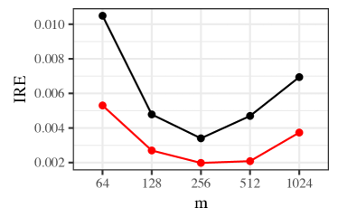
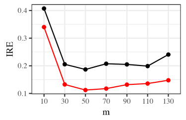
Figure 1. Average IRE of $(\sigma_{\eta},\sigma_{\xi},Z_{1},Z_{100})$ in the Poisson model with BSF (left) and of $(\phi,\sigma_{\eta},\nu,Z_{1},Z_{5473})$ in the SV model with $\psi$-APF (right). DA is shown in black and IS2 in red.

The discretely observed geometric Brownian motion example illustrated the potential gains which may be achieved by using the IS2 method in a parallel environment. While we admit that our experiment is academic, we believe that it is indicative, and shows that IS2 can provide substantial gains, and makes reliable inference possible in a much shorter time than DA. The IS framework is less prone to issues with burn-in bias, which can be problematic with naive MCMC parallelisation based on independent chains.

11. Discussion

Our framework of IS type estimators based on approximate marginal MCMC provides a general way to construct consistent estimators. Our experiments demonstrate that the IS estimator can provide substantial speedup relative to a delayed acceptance (DA) analogue with parallel computing, and appears to be competitive to DA even without parallelisation. We believe that IS is often better than DA in practice, but it is not hard to find simple examples where DA can be arbitrarily better than IS (and vice versa) [36]. Our followup work [36] complements our findings by theoretical considerations, with guaranteed asymptotic variance bounds between IS and DA.

IS is known to be difficult to implement efficiently in high dimensions, but this is not a major concern in most latent variable models, where the hyperparameters are low-dimensional. It is also generally desirable to design the approximate marginal $\pi_{a}$ to have heavier tails than the desired marginal $\pi_{m}$, in order to guarantee bounded (expected) weights. When the method of Section 2 is used, the IS weight may be directly regularised by inflating the (estimated) approximate likelihood, for instance with $L_{a}(\theta)+\epsilon$, with some $\epsilon>0$. If the likelihood $L$ is bounded, then $w_{u}(\theta)\propto L(\theta)/(L_{a}(\theta)+\epsilon)$ is bounded as well. The latter approach can be seen as an instance of defensive importance sampling [50], using the prior as a proposal component. Other generic safe IS schemes may also be useful [cf. 77], and tempering may be applied for the likelihood as well.

We used adaptive MCMC in order to construct the marginal chain $(\Theta_{k})_{k\geq 1}$ in our experiments, and believe that it is often useful [cf. 5]. Note, however, that our theoretical results do not apply directly with adaptive MCMC, unless the adaptation is stopped after suitable burn-in. Our results could be extended to hold with continuous adaptation, under certain technical conditions. We detailed proper weighting schemes based on standard IS and particle filters. We note that various PF variations, such as Rao-Blackwellisation, alternative resampling strategies [12], or quasi-Monte Carlo updates [37], apply directly. PFs can also be useful beyond the state space models context [17]. Twisted particle filters [103, 1] could also be applied, instead of the $\psi$-APF.

In a diffusion context, a proper weighting can be constructed based on randomised multilevel Monte Carlo, as recently described in [35], and ABC post-correction may be seen as IS-type correction [100]. Laplace approximations are available for a wider class of Gaussian latent variable models beyond SSMs [cf. 87]. Variational approximations [8, 57] and expectation propagation [73] have been found useful in a wide variety of models. In the SSM context, various non-linear filters could also be applied [cf. 88]. Our framework provides a generic validation mechanism for approximate inference, where assessment of bias is difficult in general [cf. 76]. Contrary to purely approximate inference, our approach only requires moderately accurate approximations, as demonstrated by our experiment with global Laplace approximations. Debiased MCMC, as suggested in [40] and further explored in [51, 52], may also lead to useful proper weighting schemes.

Appendix A Properties of augmented Markov chains

Throughout this section, suppose that $K$ is a Markov kernel on $\mathsf{X}$ and $Q$ is a kernel from $\mathsf{X}$ to a space $\mathsf{S}$. We consider here properties of an augmented Markov kernel $\check{K}$ defined on $\mathsf{X}\times\mathsf{S}$ as follows:

$$\check{K}\big{(}(x,s),\mathrm{d}x^{\prime}\times\mathrm{d}s^{\prime}\big{)}\mathrel{\mathop{:}}=K(x,\mathrm{d}x^{\prime})Q(x^{\prime},\mathrm{d}s^{\prime}).$$

We first state the following basic result.

Lemma 21.

The properties of $K$ and the augmented chain $\check{K}$ are related as follows:

1. Let $\mathrm{irr}(K)$ denote the set of $\phi$-irreducibility measures of a Markov kernel $K$, then

   • $\varphi_{K}\in\mathrm{irr}(K)\implies\varphi_{\check{K}}(\mathrm{d}x\times\mathrm{d}s)\mathrel{\mathop{:}}=\varphi_{K}(\mathrm{d}x)Q(x,\mathrm{d}s)\in\mathrm{irr}(\check{K})$,

   • $\varphi_{\check{K}}\in\mathrm{irr}(\check{K})\implies\varphi_{K}(\mathrm{d}x)\mathrel{\mathop{:}}=\varphi_{\check{K}}(\mathrm{d}x\times\mathsf{S})\in\mathrm{irr}(K)$.

2. The implications in ((i)) hold when $\mathrm{irr}(K)$ and $\mathrm{irr}(\check{K})$ are replaced with sets of maximal irreducibility measures of $K$ and $\check{K}$, respectively.

3. The invariant probabilities of $K$ and $\check{K}$ satisfy:

   • $\nu K=\nu\implies\check{\nu}\check{K}=\check{\nu}\quad\text{where}\quad\check{\nu}(\mathrm{d}x\times\mathrm{d}y)\mathrel{\mathop{:}}=\nu(\mathrm{d}x)Q(x,\mathrm{d}y)$,

   • $\check{\nu}\check{K}=\check{\nu}\implies\nu K=\nu\quad\text{where}\quad\nu(\mathrm{d}x)\mathrel{\mathop{:}}=\check{\nu}(\mathrm{d}x\times\mathsf{S})$.

   These implications hold also with invariance replaced by reversibility.

4. $K$ is Harris recurrent if and only if $\check{K}$ is Harris recurrent.

5. Suppose $h:\mathsf{X}\times\mathsf{S}\to\mathbb{R}$ is measurable and such that $m_{h}(x)\mathrel{\mathop{:}}=\int Q(x,\mathrm{d}s)h(x,s)$ and $(K^{n}m_{h})(x)$ are well-defined. Then, for any $n\geq 1$ and $s\in\mathsf{S}$, $(\check{K}^{n}h)(x,s)=(K^{n}m_{h})(x)$.

Proof.

The inheritance of irreducibility measures (i), maximal irreducibility measures (ii), invariant measures (iii), and reversibility is straightforward.

For Harris recurrence (iv), let the probability $\phi_{K}$ be a maximal irreducibility measure for $K$, then $\phi_{\check{K}}(\mathrm{d}x\times\mathrm{d}s)\mathrel{\mathop{:}}=\phi_{K}(\mathrm{d}x)Q(x,\mathrm{d}s)$ is the maximal irreducibility measure for $\check{K}$. Let $C\in\mathcal{X}\otimes\mathcal{S}$ with $\phi_{\check{K}}(C)>0$, and choose $\epsilon>0$ such that $\phi_{K}(C(\epsilon))>0$, where $C(\epsilon)\mathrel{\mathop{:}}=\{x\in\mathsf{X}\,:\,Q(x,C_{x})>\epsilon\}$ with $C_{x}\mathrel{\mathop{:}}=\{s\in\mathsf{S}\,:\,(x,s)\in C\}$. Notice that

$$\mathbb{P}\bigg{(}\sum_{k=1}^{\infty}\mathbb{I}\left((X_{k},S_{k})\in C\right)=\infty\bigg{)} \geq\mathbb{P}\bigg{(}\sum_{k=1}^{\infty}\mathbb{I}\left(S_{\tau_{k}}\in C_{X_{\tau_{k}}}\right)=\infty\bigg{)},$$

where $\tau_{k}$ are the hitting times of $(X_{k})$ to $C(\epsilon)$. This concludes the proof because $\mathbb{I}\left(S_{\tau_{k}}\in C_{X_{\tau_{k}}}\right)$ are independent Bernoulli random variables with success probability at least $\epsilon$. The converse statement is similar.

For (v), it is enough to notice that for any $(x,s)\in\mathsf{X}\times\mathsf{S}$ and $n\geq 1$, it holds that $\check{K}^{n}\big{(}(x,s),\mathrm{d}x^{\prime}\times\mathrm{d}s^{\prime}\big{)}=K^{n}(x,\mathrm{d}x^{\prime})Q(x^{\prime},\mathrm{d}s)$. ∎

We next state the following generic results about the asymptotic variance and the central limit theorem of an augmented Markov chain. For $h\in L_{0}^{2}(\check{\nu})$, we denote as above the conditional mean $m_{h}(x)\mathrel{\mathop{:}}=\int Q(x,\mathrm{d}s)h(x,s)$ and the conditional variance $v_{h}(x)\mathrel{\mathop{:}}=\int Q(x,\mathrm{d}s)h^{2}(x,s)-m_{h}^{2}(x)$.

Lemma 22.

Let $h\in L_{0}^{2}(\check{\nu})$. The asymptotic variance of an augmented Markov chain satisfies

$$\mathrm{Var}(h,\check{K})=\mathrm{Var}(m_{h},K)+\nu(v_{h}),$$

whenever $\mathrm{Var}(m_{h},K)$ is well-defined.

Proof.

Let $(X_{k},S_{k})$ be a stationary Markov chain with transition probability $\check{K}$.

$$\mathrm{Var}\bigg{(}\frac{1}{\sqrt{n}}\sum_{k=1}^{n}h(X_{k},S_{k})\bigg{)} =\check{\nu}(h^{2})+\frac{2}{n}\sum_{i=1}^{n-1}\sum_{\ell=1}^{n-i}\mathbb{E}[h(X_{0},S_{0})h(X_{\ell},S_{\ell})],$$

by stationarity. For $\ell\geq 1$, Lemma 21 (v) implies

$$\mathbb{E}[h(X_{0},S_{0})h(X_{\ell},S_{\ell})] =\mathbb{E}[m_{h}(X_{0})m_{h}(X_{\ell})].$$

We deduce for any $n\geq 1$

$$\mathrm{Var}\bigg{(}\frac{1}{\sqrt{n}}\sum_{k=1}^{n}h(X_{k},S_{k})\bigg{)}=\mathrm{Var}\bigg{(}\frac{1}{\sqrt{n}}\sum_{k=1}^{n}m_{h}(X_{k})\bigg{)}+\nu(v_{h}),$$

because $\check{\nu}(h^{2})-\nu(m_{h}^{2})=\nu(v_{h})$. The claim follows by taking limit $n\to\infty$. ∎

Lemma 23.

Suppose $K$ is Harris ergodic and aperiodic, and $h\in L_{0}^{2}(\check{\nu})$. The CLT

(10) $$Z_{n}\mathrel{\mathop{:}}=\frac{1}{\sqrt{n}}\sum_{k=1}^{n}h(X_{k},S_{k})\xrightarrow{n\to\infty}N\big{(}0,\sigma_{h}^{2}\big{)},\qquad\text{where}\qquad\sigma_{h}^{2}\mathrel{\mathop{:}}=\mathrm{Var}(m_{h},K)+\nu(v_{h})$$

holds for every initial distribution, if one of the following holds:

1. $K$ is reversible and $\mathrm{Var}(m_{h},K)<\infty$.

2. $\sum_{n=1}^{\infty}n^{-3/2}\big{\{}\nu\big{(}\big{[}\sum_{i=0}^{n-1}K^{i}m_{h}\big{]}^{2}\big{)}\big{\}}^{1/2}<\infty$.

3. There exists $g\in L^{2}(\nu)$ which solves the Poisson equation $g-Kg=m_{h}$. In this case, $\mathrm{Var}(m_{h},K)=\nu(g^{2}-(Kg)^{2})$.

Proof.

The case (i) follows from Lemma 22 and the Kipnis-Varadhan CLT [59], which implies (10) for the initial distribution $\check{\nu}$. Because the jump chain is Harris by Lemma 21 (iv), (10) holds for every initial distribution [23, Corollary 21.1.6].

The case (ii) follows similarly, but relies on a result due to Maxwell and Woodroofe [70], which implies (10) for the initial distribution $\check{\nu}$, if $\sum_{n=1}^{\infty}n^{-3/2}\big{\{}\check{\nu}\big{(}\big{[}\sum_{i=0}^{n-1}\check{K}^{i}h\big{]}^{2}\big{)}\big{\}}^{1/2}<\infty$. Notice that for $n\geq 2$ by Lemma 21 (v),

$$\check{\nu}\bigg{(}\bigg{[}\sum_{i=0}^{n-1}\check{K}^{i}h\bigg{]}^{2}\bigg{)} =\check{\nu}\bigg{(}\bigg{[}(h-m_{h})+\sum_{i=0}^{n-1}K^{i}m_{h}\bigg{]}^{2}\bigg{)}=\nu(v_{h})+\nu\bigg{(}\bigg{[}\sum_{i=0}^{n-1}K^{i}m_{h}\bigg{]}^{2}\bigg{)}.$$

Because $(a+b)^{1/2}\leq a^{1/2}+b^{1/2}$ for $a,b\geq 0$ and $\nu(v_{h})<\infty$, the claim follows.

For (iii), we first observe that

$$\check{g}-\check{K}\check{g}=h\qquad\text{where}\qquad\check{g}(x,s)\mathrel{\mathop{:}}=g(x)+h(x,s)-m_{h}(x)\in L^{2}(\check{\nu}).$$

Indeed, it is clear that $\check{g}\in L^{2}(\check{\nu})$ and because $(\check{K}\check{g})(x,s)=(Kg)(x)$,

$$\check{g}(x,s)-(\check{K}\check{g})(x,s)=g(x)-(Kg)(x)+h(x,s)-m_{h}(x)=h(x,s).$$

The CLT and asymptotic variance follow from [72, Theorem 17.4.4]. ∎

Appendix B Proofs about CLT and asymptotic variance

Proof of Theorem 7.

Whenever $\sum_{i=1}^{n}\xi_{i}(\mathbf{1})>0$, we may write

(11) $$\sqrt{n}\big{[}E_{n}(f)-\pi(f)\big{]}=\frac{n^{-1/2}\sum_{k=1}^{n}\xi_{k}(\bar{f})}{n^{-1}\sum_{j=1}^{n}\xi_{j}(\mathbf{1})}.$$

The denominator converges to $c_{w}>0$ almost surely, so by Slutsky’s lemma, it is enough to show that the numerator converges in distribution to $N\big{(}0,\mathrm{Var}(\nu_{\bar{f}},P)+\pi_{a}(v)\big{)}$. This follows from Lemma 23 (i) and (ii), under conditions (i) and (ii), respectively. ∎

Proof of Corollary 9.

If $\sqrt{n}\big{[}E_{n}(f)-\pi(f)\big{]}\to N(0,\sigma_{f}^{2})$, Slutsky’s lemma applied to (11) implies that $n^{-1/2}\sum_{k=1}^{n}\xi_{k}(\bar{f})\to N(0,c_{w}^{2}\sigma_{f}^{2})$. Consistency of the integrated autocovariance estimator implies $\hat{a}_{n}\to\sum_{k=-\infty}^{\infty}\gamma_{k}=c_{w}^{2}\sigma_{f}^{2}$, and therefore $\hat{s}_{n}\to\sigma_{f}^{2}$. The conclusion follows by a standard continuity argument. ∎

Proof of Theorem 10.

For $n$ large enough such that $\sum_{j=1}^{n}\xi_{j}(\mathbf{1})>0$, we may write

$$n\hat{v}_{n}=\frac{\frac{1}{n}\sum_{k=1}^{n}\big{(}\xi_{k}(f)-\xi_{k}(\mathbf{1})E_{n}(f)\big{)}^{2}}{\big{(}\frac{1}{n}\sum_{j=1}^{n}\xi_{j}(\mathbf{1})\big{)}^{2}}.$$

The denominator converges to $c_{w}^{2}$, and the numerator can be written as

$$\frac{1}{n}\sum_{k=1}^{n}\big{[}\xi_{k}^{2}(\bar{f})+\xi_{k}^{2}(\mathbf{1})D_{n}^{2}+2\xi_{k}(\mathbf{1})\xi_{k}(\bar{f})D_{n}\big{]}\qquad\text{with}\qquad D_{n}\mathrel{\mathop{:}}=\pi(f)-E_{n}(f).$$

The term $n^{-1}\sum_{k=1}^{n}\xi_{k}^{2}(\bar{f})\to\pi_{a}(v+\mu_{\bar{f}}^{2})$, and because $D_{n}\to 0$, the remainder terms tend to zero. ∎

Appendix C Proofs about jump chain estimators

In this section, $K$ is assumed to be a Markov kernel on $\mathsf{X}$ which is non-degenerate, that is, $a(x)\mathrel{\mathop{:}}=K(x,\mathsf{X}\setminus\{x\})>0$ for all $x\in\mathsf{X}$. The following proposition complements [24, Lemma 1] and [19], which are stated for more specific cases.

Proposition 24.

Suppose $(X_{k})$ is a Markov chain with kernel $K$ and $(\tilde{X}_{k})$ the corresponding jump chain with holding times $(N_{k})$ (Definition 4). Then, the following hold:

1. $(\tilde{X}_{k})$ is Markov with transition kernel $\tilde{K}(x,A)=K(x,A\setminus\{x\})/a(x)$.

2. The holding times $(N_{k})$ are conditionally independent given $(\tilde{X}_{k})$, and each $N_{k}$ has geometric distribution with parameter $a(\tilde{X}_{k})$.

3. If $K$ admits invariant probability $\nu(\mathrm{d}x)$, then $\tilde{K}$ admits invariant probability $\tilde{\nu}(\mathrm{d}x)\mathrel{\mathop{:}}=\nu(\mathrm{d}x)a(x)/\nu(a).$ In addition, if $K$ is reversible with respect to $\nu$, then $\tilde{K}$ is reversible with respect to $\tilde{\nu}$.

4. $(X_{k})$ is $\psi$-irreducible if and only if $(\tilde{X}_{k})$ is $\psi$-irreducible, with the same maximal irreducibility measure.

5. $(X_{k})$ is Harris recurrent if and only if $(\tilde{X}_{k})$ is Harris recurrent.

Proof.

The expression of the kernel (i) is due to straightforward conditioning, and (ii) was observed in [24]. The invariance (iii) follows from

$$\int\tilde{\nu}(\mathrm{d}x)\tilde{K}(x,A) =\frac{1}{\nu(a)}\int\nu(\mathrm{d}x)\big{[}K(x,A)-\mathbb{I}\left(x\in A\right)K(x,\{x\})\big{]}$$

$$=\frac{1}{\nu(a)}\bigg{[}\nu(A)-\int_{A}\nu(\mathrm{d}x)\big{(}1-a(x)\big{)}\bigg{]}=\tilde{\nu}(A),$$

and the reversibility is shown in [24]. For (iv) it is sufficient to observe that

$$\forall x\in\mathsf{X}:\sum_{n\geq 1}\mathbb{P}_{x}(X_{n}\in A)>0\iff\forall x\in\mathsf{X}:\sum_{n\geq 1}\mathbb{P}_{x}(\tilde{X}_{n}\in A)>0,$$

where $\mathbb{P}_{x}(\,\cdot\,)=\mathbb{P}(\,\cdot\,\mid X_{0}=\tilde{X}_{0}=x)$, which holds because the sets $\{X_{k}\}_{k\geq 0}$ and $\{\tilde{X}_{k}\}_{k\geq 0}$ coincide. Similarly, (v) holds because

$$\forall x\in\mathsf{X}:\mathbb{P}_{x}(\eta_{A}=\infty)=1\iff\forall x\in\mathsf{X}:\mathbb{P}_{x}(\tilde{\eta}_{A}=\infty)=1,$$

where $\eta_{A}\mathrel{\mathop{:}}=\sum_{k=1}^{\infty}\mathbb{I}\left(X_{k}\in A\right)$ and $\tilde{\eta}_{A}\mathrel{\mathop{:}}=\sum_{k=1}^{\infty}\mathbb{I}\left(\smash{\tilde{X}_{k}\in A}\right)$. ∎

We now state results about the asymptotic variance of the jump chain, complementing the reversible case characterisation of [19, 28].

Proposition 25.

Let $f\in L^{2}_{0}(\tilde{\nu})$. With the notation of Proposition 24,

1. If $K$ is reversible, then $\mathrm{Var}(f,\tilde{K})<\infty$ iff $af\in L^{2}(\nu)$ and $\mathrm{Var}(af,K)<\infty$, and

   (12) $$\mathrm{Var}(f,\tilde{K})=\nu(a)^{-1}\big{[}\mathrm{Var}(af,K)-\nu\big{(}a(1-a)f^{2}\big{)}\big{]}.$$

2. If there exists a function $g\in L^{2}(\nu)$ which satisfies $g-Kg=af$, then $\mathrm{Var}(f,\tilde{K})<\infty$, $\mathrm{Var}(af,K)<\infty$, (12) holds, $g-\tilde{K}g=f$ and $g\in L^{2}(\tilde{\nu})$.

Proof.

The reversible case (i) is a restatement of [19, Theorem 1].

Consider then (ii). By Proposition 24 (i), we obtain for any $h:\mathsf{X}\to\mathbb{R}$ with $Kh$ well-defined,

$$(\tilde{K}h)(x)=\frac{(Kh)(x)-\big{(}1-a(x)\big{)}h(x)}{a(x)}=\frac{(Kh)(x)-h(x)}{a(x)}+h(x).$$

Consequently, we observe that $g-\tilde{K}g=a^{-1}\big{(}g-Kg\big{)}=f$ implying (ii). Because $g\in L^{2}(\tilde{\nu})$, Lemma 23 (iii) and a straightforward calculation yield

$$\mathrm{Var}(f,\tilde{K}) =\tilde{\nu}\big{(}g^{2}-(\tilde{K}g)^{2}\big{)}$$

$$=2\langle g,g-\tilde{K}g\rangle_{\tilde{\nu}}-\langle g-\tilde{K}g,g-\tilde{K}g\rangle_{\tilde{\nu}}$$

$$=\nu(a)^{-1}\big{[}2\langle g,g-Kg\rangle_{\nu}-\nu(af^{2})\big{]},$$

where $\langle f,g\rangle_{\nu}\mathrel{\mathop{:}}=\int f(x)g(x)\nu(\mathrm{d}x)$. Similarly, by Lemma 23 (iii)

$$\mathrm{Var}(af,K)=\nu\big{(}g^{2}-(Kg)^{2}\big{)}=2\langle g,g-Kg\rangle_{\nu}-\nu(a^{2}f^{2}),$$

which allows us to conclude. ∎

Proof of Theorem 15.

Whenever $\sum_{j=1}^{n}\xi_{j}(\mathbf{1})>0$, we may write

$$\sqrt{n}\big{[}E_{n}(f)-\pi(f)\big{]}=\frac{n^{-1/2}\sum_{k=1}^{n}N_{k}\xi_{k}(\bar{f})}{n^{-1}\sum_{j=1}^{n}N_{j}\xi_{j}(\mathbf{1})}.$$

We shall show below that the CLT holds for the numerator, with asymptotic variance $\sigma^{2}\mathrel{\mathop{:}}=\big{[}\mathrm{Var}(\mu_{\bar{f}},P)+\pi_{a}(\alpha\tilde{v})\big{]}/\pi_{a}(\alpha)$. This implies the claim by Slutsky’s lemma, as the denominator converges to $c_{w}/\pi_{a}(\alpha)$. For the rest of the proof, let $\tilde{P}$ and $\check{P}$ be the Markov kernels of $(\tilde{\Theta}_{k})_{k\geq 1}$ and $(\tilde{\Theta}_{k}$,$N_{k}$,$\xi_{k}(\bar{f}))_{k\geq 1}$, respectively, and let $\tilde{\pi}$ and $\check{\pi}$ be the corresponding invariant probabilities. Note that the function $h(\theta,n,\xi)\mathrel{\mathop{:}}=n\xi$ is in $L^{2}(\check{\pi})$ by assumption (6).

In case (i) holds, also $\tilde{P}$ and $\check{P}$ are reversible by Proposition 24 (iii) and Lemma 21 (iii). Lemma 23 (i) with $K=\tilde{P}$, $\check{K}=\check{P}$, $\nu=\tilde{\pi}$ and $\check{\nu}=\check{\pi}$ implies that a CLT holds for $h$ whenever the asymptotic variance is finite:

$$\mathrm{Var}(h,\check{P})=\mathrm{Var}\big{(}\mu_{\bar{f}}/\alpha,\tilde{P}\big{)}+\pi_{a}(\alpha\tilde{v}_{N\xi})/\pi_{a}(\alpha),$$

where, by the variance decomposition formula,

$$\tilde{v}_{N\xi}(\theta) \mathrel{\mathop{:}}=\mathrm{Var}(N_{k}\xi_{k}(\bar{f})\mid\tilde{\Theta}_{k}=\theta)$$

$$=\tilde{v}(\theta)+\mathrm{Var}\big{(}N_{k}\mathbb{E}[\xi_{k}(\bar{f})\mid\tilde{\Theta}_{k}=\theta,N_{k}]\mathrel{\big{|}}\tilde{\Theta}_{k}=\theta\big{)}$$

$$=\tilde{v}(\theta)+\mu_{\bar{f}}^{2}(\theta)\big{(}1-\alpha(\theta)\big{)}/\alpha^{2}(\theta).$$

Proposition 25 (i) implies that

$$\mathrm{Var}\big{(}\mu_{\bar{f}}/\alpha,\tilde{P}\big{)}=\pi_{a}(\alpha)^{-1}\big{[}\mathrm{Var}(\mu_{\bar{f}},P)-\pi_{a}\big{(}(1-\alpha)\mu_{\bar{f}}^{2}/\alpha\big{)}\big{]},$$

which implies $\mathrm{Var}(h,\check{P})=\sigma^{2}$.

Consider then (ii). Proposition 25 (ii) implies that $g-\tilde{P}g=\mu_{\bar{f}}/\alpha$, and $g\in L^{2}(\tilde{\pi})$. Lemma 23 (iii) implies the CLT, and together with Proposition 25 (ii) leads to $\mathrm{Var}(h,\check{P})=\sigma^{2}$. ∎

Appendix D Proper weightings for general state space models

We review some techniques to construct proper weightings in case of general state-space models introduced in Section 8. First, note that the simple IS correction may be applied directly (see Proposition 4). Note that (8) is satisfied for all integrable $h$, so $\mathcal{L}=L^{1}(\pi)$. It is often useful to combine such schemes as in Proposition 6, allowing for instance variance reduction by using pairs of antithetic variables [30].

For the rest of the section, we focus on the particle filter (PF) algorithm [44]; see also the monographs [25, 16, 12]. We consider a generic version of the algorithm, with the following components [cf. 16]:

1. Proposal distributions: $M_{1}$ is a probability density on $\mathsf{S}_{z}$ and $M_{t}(\,\cdot\,\mid z_{1:t-1})$ defines conditional densities on $\mathsf{S}_{z}$ given $z_{1:t-1}\in\mathsf{S}_{z}^{t-1}$.

2. Potential functions: $G_{t}:\mathsf{S}_{z}^{t}\to\mathbb{R}_{+}$.

3. Resampling laws: $\mathrm{Res}(\,\cdot\,\mid\bar{\omega}^{(1:m)})$ defines a probability distribution on $\{1{:}m\}^{m}$ for every discrete probability mass $\bar{\omega}^{(1:m)}$.

The following well-known two conditions are minimal to ensure unbiasedness, which is required for proper weighting:

Assumption 6.

Suppose that the following hold:

1. $\prod_{t=1}^{T}M_{t}(z_{t}\mid z_{1:t-1})G_{t}(z_{1:t})\ =p^{(\theta)}(z_{1:T},y_{1:T})$ for all $z_{1:T}\in\mathsf{S}_{z}^{T}$.

2. $\mathbb{E}\big{[}\sum_{i=1}^{m}\mathbb{I}\left(\vphantom{(}\smash{A^{(i)}=j}\right)\big{]}=m\bar{\omega}^{(j)}$, where $A^{(1:m)}\sim\mathrm{Res}(\,\cdot\,\mid\bar{\omega}^{(1:m)})$, for any $j\in\{1{:}m\}$ and any probability mass vector $\bar{\omega}^{(1:m)}$.

Assumption 6 (i) holds with traditionally used ‘filtering’ potentials $G_{t}(z_{1:t})\mathrel{\mathop{:}}=g_{t}^{(\theta)}(y_{t}\mid z_{t})\mu_{t}^{(\theta)}(z_{t}\mid z_{t-1})/M_{t}(z_{t}\mid z_{1:t-1})$, assuming a suitable support condition. We discuss another choice of $M_{t}$ and $G_{t}$ in Section 8, inspired by the ‘twisted SSM’ approach of [46]. It allows a ‘look-ahead’ strategy based on approximations of the full smoothing distributions $q^{(\theta)}(z_{1:T}\mid y_{1:T})$. Assumption 6 (ii) allows for multinomial resampling, where $A_{t}^{(i)}$ are independent draws from $\bar{\omega}_{t}^{(1:m)}$, but also for lower variance schemes, including stratified, residual and systematic resampling methods [cf. 22].

Below, whenever the index ‘$i$’ appears, it takes values $i=1,\ldots,m$.

Algorithm 1 (Particle filter).

Initial state:

1. Sample $Z_{1}^{(i)}\sim M_{1}$ and set $\bar{Z}_{1}^{(i)}=Z_{1}^{(i)}$.

2. Calculate $\omega_{1}^{(i)}\mathrel{\mathop{:}}=G_{1}(Z_{1}^{(i)})$ and set $\bar{\omega}_{1}^{(i)}\mathrel{\mathop{:}}=\omega_{1}^{(i)}/\omega_{1}^{*}$ where $\omega_{1}^{*}=\sum_{j=1}^{m}\omega_{1}^{(j)}$.

For $t=2,\ldots,T$, do:

1. Sample $A_{t-1}^{(1:m)}\sim\mathrm{Res}(\,\cdot\,\mid\bar{\omega}_{t-1}^{(1:m)})$.

2. Sample $Z_{t}^{(i)}\sim M_{t}(\,\cdot\,\mid\bar{Z}_{t-1}^{(A_{t-1}^{(i)})})$ and set $\bar{Z}_{t}^{(i)}=(\bar{Z}_{t-1}^{(A_{t-1}^{(i)})},Z_{t}^{(i)})$.

3. Calculate $\omega_{t}^{(i)}\mathrel{\mathop{:}}=G_{t}(\bar{Z}_{t-1}^{(A_{t-1}^{(i)})},Z_{t})$ and set $\bar{\omega}_{t}^{(i)}\mathrel{\mathop{:}}=\omega_{t}^{(i)}/\omega_{t}^{*}$ where $\omega_{t}^{*}=\sum_{j=1}^{m}\omega_{t}^{(j)}$.

Remark 26.

If all weights are zero, $\omega_{t}^{*}=0$, then Algorithm 1 may be terminated immediately (cf. Proposition 27).

The following result summarises alternative ways how the random variables $(V^{(1:m)}_{\theta},X^{(1:m)}_{\theta})$ may be constructed from the PF output, in order to satisfy (8). The results stated below are gathered from the literature [e.g. 16, 79], and some may be stated under slightly more stringent conditions; a self-contained proof of Proposition 27 may be found, for instance, in [101].

Proposition 27.

Let $\theta\in\mathsf{T}$ be fixed, assume $\mathrm{Res}$, $M_{t}$ and $G_{t}$ satisfy Assumption 6, and let $h:\mathsf{S}_{z}^{T}\to\mathbb{R}$ be such that the integral in (8) is well-defined and finite. Consider the random variables generated by Algorithm 1, and let $U\mathrel{\mathop{:}}=\prod_{t=1}^{T}\big{(}\frac{1}{m}\omega_{t}^{*}\big{)}$. Then,

1. the random variables $(V^{(1:m)}_{\theta},X^{(1:m)}_{\theta})$ where $V^{(i)}_{\theta}=U\bar{\omega}_{T}^{(i)}$ and $X^{(i)}_{\theta}=\bar{Z}_{T}^{(i)}$ satisfy (8).

Suppose in addition that $M_{t}(z_{t}\mid z_{1:t-1})G_{t}(z_{1:t})=C_{t}(z_{t-1:t})$ for all $t\in\{1{:}T\}$ and all $z_{1:T}\in\mathsf{S}_{z}^{T}$. Define for $t\in\{2{:}T\}$, and any $i_{t},i_{t-1}\in\{1{:}m\}$, the backwards sampling probabilities

$$b_{t-1}(i_{t-1}\mid i_{t})\mathrel{\mathop{:}}=\frac{\bar{\omega}_{t-1}^{(i_{t-1})}C_{t}(Z_{t-1}^{(i_{t-1})},Z_{t}^{(i_{t})})}{\sum_{\ell=1}^{m}\bar{\omega}_{t-1}^{(\ell)}C_{t}(Z_{t-1}^{(\ell)},Z_{t}^{(i_{t})})},\quad\text{and}\quad b_{T}(i_{T}\mid i_{T+1})=\bar{\omega}_{T}^{(i_{T})}.$$

1. Let $I_{1:T}$ be random indices generated recursively backwards by $I_{T}\sim b_{T}$ and $I_{t}\sim b_{t}(\,\cdot\,\mid I_{t+1})$. The random variables $(V^{(1)}_{\theta},X^{(1)}_{\theta})$ satisfy (8), where $V^{(1)}_{\theta}=U$ and $X^{(1)}_{\theta}=Z_{1:T}^{(I_{1:T})}$.

2. If $h(z_{1:T})=\hat{h}(z_{t-1},z_{t})$ for some $t\in\{2{:}T\}$, that is, $h$ is constant in all coordinates except $t-1$ and $t$, then, the random variables $(V^{(1:m,1:m)}_{\theta}$, $X^{(1:m,1:m)}_{\theta})$ satisfy (8) (with $\hat{h}$ on the left), where

   1. $X^{(i,j)}_{\theta}\mathrel{\mathop{:}}=(Z_{t-1}^{(i)},Z_{t}^{(j)})$,

   2. $V^{(i,j)}_{\theta}\mathrel{\mathop{:}}=Ub_{t-1}(i\mid j)\hat{\omega}_{t}^{(j)}$, and where

   3. $\hat{\omega}_{T}^{(i)}\mathrel{\mathop{:}}=\bar{\omega}_{T}^{(i)}$ and $\hat{\omega}_{t}^{(i)}\mathrel{\mathop{:}}=\sum_{k=1}^{m}\hat{\omega}_{t+1}^{(k)}b_{t}(i\mid k)$ for $t=T-1,\ldots,t$.

3. If $h(z_{1:T})=\hat{h}(z_{t})$ for some $t\in\{1{:}T\}$, then the random variables $(V^{(1:m)}_{\theta},X^{(1:m)}_{\theta})$ satisfy (8) (with $\hat{h}$ on the left), where $X^{(i)}_{\theta}=Z_{t}^{(i)}$ and $V^{(i)}_{\theta}=U\hat{\omega}_{t}^{(i)}$ are defined in (iii)c.

The estimator in Proposition 27 (i) was called the filter-smoother in [60]. This property was shown in [16, Theorem 7.4.2] in case of multinomial resampling, and extended later [cf. 2]. Proposition 27 (ii) corresponds to backwards simulation smoothing [42]. Drawing a single backward trajectory does not improve on the filter-smoother [cf. 27], but drawing several $I_{1:T}$ independently may lead to lower variance estimators. Proposition 27 (iii) and its special case (iv) correspond to the forward-backward smoother [26]; see also [12]. It is a Rao-Blackwellised version of (ii), but applicable only when considering estimates of a single marginal (pair). This scheme can lead to lower variance, but suffers from $O(m^{2})$ complexity.

We next formally state how Proposition 27 allows to use Algorithm 1 to derive a proper weighting scheme.

Corollary 28.

Let $(\Theta_{k})_{k\geq 1}$ be a Markov chain which is Harris ergodic with respect to $\pi_{a}$. Suppose each $(V^{(1:m)}_{k},X^{(1:m)}_{k})$ corresponds to an independent run of Algorithm 1 with $\theta=\Theta_{k}$, as defined in Proposition 27 (i), (ii), (iii) or (iv). Then, $(W_{k}^{(1:m)},X^{(1:m)}_{k})_{k\geq 1}$ with $W_{k}^{(i)}\mathrel{\mathop{:}}=\mathrm{pr}(\theta_{k})V_{k}^{(i)}/\pi_{a}(\theta_{k})$ provide a proper weighting scheme for target distribution $\pi(\theta,x_{1:T})=p(\theta,x_{1:T}\mid y_{1:T})$ (Definition 2), for the following classes of functions, respectively:

$$\ref{item:filter-smoother}\quad\mathcal{L} =L^{1}(\pi), \ref{item:fwd-bwd-smoothing}\quad\mathcal{L} =\big{\{}f\in L^{1}(\pi)\,:\,f(\theta,x_{1:T})=f(\theta,x_{t-1:t}),\text{ for some $t\in\{2{:}T\}$}\big{\}},$$

$$\ref{item:backwards-sampling}\quad\mathcal{L} =L^{1}(\pi), \ref{item:fwd-bwd-smoothing2}\quad\mathcal{L} =\big{\{}f\in L^{1}(\pi)\,:\,f(\theta,x_{1:T})=f(\theta,x_{t}),\text{ for some $t\in\{1{:}T\}$}\big{\}}.$$

In case $(\Theta_{k},U_{k})_{k\geq 1}$ is a pseudo-marginal algorithm, $W_{k}\mathrel{\mathop{:}}=\mathrm{pr}(\theta_{k})V_{k}^{(i)}/U_{k}$.

References

- [1] J. Ala-Luhtala, N. Whiteley, K. Heine, and R. Piché. An introduction to twisted particle filters and parameter estimation in non-linear state-space models. IEEE Trans. Signal Process., 64(18):4875–4890, 2016.
- [2] C. Andrieu, A. Doucet, and R. Holenstein. Particle Markov chain Monte Carlo methods. J. R. Stat. Soc. Ser. B Stat. Methodol., 72(3):269–342, 2010.
- [3] C. Andrieu, A. Lee, and M. Vihola. Uniform ergodicity of the iterated conditional SMC and geometric ergodicity of particle Gibbs samplers. Bernoulli, 24(2):842–872, 2018.
- [4] C. Andrieu and G. O. Roberts. The pseudo-marginal approach for efficient Monte Carlo computations. Ann. Statist., 37(2):697–725, 2009.
- [5] C. Andrieu and J. Thoms. A tutorial on adaptive MCMC. Statist. Comput., 18(4):343–373, Dec. 2008.
- [6] C. Andrieu and M. Vihola. Convergence properties of pseudo-marginal Markov chain Monte Carlo algorithms. Ann. Appl. Probab., 25(2):1030–1077, 2015.
- [7] C. Andrieu and M. Vihola. Establishing some order amongst exact approximations of MCMCs. Ann. Appl. Probab., 26(5):2661–2696, 2016.
- [8] M. J. Beal. Variational algorithms for approximate Bayesian inference. PhD thesis, University College London, 2003.
- [9] M. A. Beaumont. Estimation of population growth or decline in genetically monitored populations. Genetics, 164:1139–1160, 2003.
- [10] A. Beskos, O. Papaspiliopoulos, G. O. Roberts, and P. Fearnhead. Exact and computationally efficient likelihood-based estimation for discretely observed diffusion processes. J. R. Stat. Soc. Ser. B Stat. Methodol., 68(3):333–382, 2006.
- [11] S. Bhattacharya. Consistent estimation of the accuracy of importance sampling using regenerative simulation. Statist. Probab. Lett., 78(15):2522–2527, 2008.
- [12] O. Cappé, E. Moulines, and T. Rydén. Inference in Hidden Markov Models. Springer, 2005.
- [13] N. Chopin, P. Jacob, and O. Papaspiliopoulos. SMC2: A sequential Monte Carlo algorithm with particle Markov chain Monte Carlo updates. J. R. Stat. Soc. Ser. B Stat. Methodol., 75(3):397–426, 2013.
- [14] N. Chopin and S. S. Singh. On particle Gibbs sampling. Bernoulli, 21(3):1855–1883, 2015.
- [15] J. A. Christen and C. Fox. Markov chain Monte Carlo using an approximation. J. Comput. Graph. Statist., 14(4), 2005.
- [16] P. Del Moral. Feynman-Kac Formulae. Springer, 2004.
- [17] P. Del Moral, A. Doucet, and A. Jasra. Sequential Monte Carlo samplers. J. R. Stat. Soc. Ser. B Stat. Methodol., 68(3):411–436, 2006.
- [18] G. Deligiannidis, A. Doucet, M. K. Pitt, and R. Kohn. The correlated pseudo-marginal method. Preprint, arXiv:1511.04992v3, 2015.
- [19] G. Deligiannidis and A. Lee. Which ergodic averages have finite asymptotic variance? Ann. Appl. Probab., 28(4):2309–2334, 2018.
- [20] H. Doss. Discussion: Markov chains for exploring posterior distributions. Ann. Statist., 22(4):1728–1734, 1994.
- [21] H. Doss. Estimation of large families of Bayes factors from Markov chain output. Statist. Sinica, pages 537–560, 2010.
- [22] R. Douc, O. Cappé, and E. Moulines. Comparison of resampling schemes for particle filtering. In Proc. Image and Signal Processing and Analysis, 2005, pages 64–69, 2005.
- [23] R. Douc, E. Moulines, P. Priouret, and P. Soulier. Markov chains. Springer, 2018.
- [24] R. Douc and C. P. Robert. A vanilla Rao-Blackwellization of Metropolis-Hastings algorithms. Ann. Statist., 39(1):261–277, 2011.
- [25] A. Doucet, N. de Freitas, and N. Gordon. Sequential Monte Carlo Methods in Practice. Springer-Verlag, New York, 2001.
- [26] A. Doucet, S. Godsill, and C. Andrieu. On sequential Monte Carlo sampling methods for Bayesian filtering. Statist. Comput., 10(3):197–208, 2000.
- [27] A. Doucet and A. Lee. Sequential Monte Carlo methods. In M. Matthuis, M. Drton, S. Lauritzen, , and M. Wainwright, editors, Handbook of Graphical Models, pages 165–188. CRC press, 2019.
- [28] A. Doucet, M. Pitt, G. Deligiannidis, and R. Kohn. Efficient implementation of Markov chain Monte Carlo when using an unbiased likelihood estimator. Biometrika, 102(2):295–313, 2015.
- [29] J. Durbin and S. J. Koopman. Monte Carlo maximum likelihood estimation for non-Gaussian state space models. Biometrika, 84(3):669–684, 1997.
- [30] J. Durbin and S. J. Koopman. Time series analysis of non-Gaussian observations based on state space models from both classical and Bayesian perspectives. J. R. Stat. Soc. Ser. B Stat. Methodol., 62:3–56, 2000.
- [31] J. Durbin and S. J. Koopman. A simple and efficient simulation smoother for state space time series analysis. Biometrika, 89:603–615, 2002.
- [32] J. Durbin and S. J. Koopman. Time series analysis by state space methods. Oxford University Press, New York, 2nd edition, 2012.
- [33] J. M. Flegal and G. L. Jones. Batch means and spectral variance estimators in Markov chain Monte Carlo. Ann. Statist., 38(2):1034–1070, 2010.
- [34] C. Fox and G. Nicholls. Sampling conductivity images via MCMC. In K. V. Mardia, C. A. Gill, and R. G. Aykroyd, editors, Proceedings in The Art and Science of Bayesian Image Analysis, pages 91–100. Leeds University Press, 1997.
- [35] J. Franks, A. Jasra, K. Law, and M. Vihola. Unbiased inference for discretely observed hidden markov model diffusions. Preprint, arXiv:1807.10259, 2018.
- [36] J. Franks and M. Vihola. Importance sampling and delayed acceptance via a Peskun type ordering. Preprint, arXiv:1706.09873, 2017.
- [37] M. Gerber and N. Chopin. Sequential quasi-Monte Carlo. J. R. Stat. Soc. Ser. B Stat. Methodol., 77(3):509–579, 2015.
- [38] M. B. Giles. Multilevel Monte Carlo path simulation. Oper. Res., 56(3):607–617, 2008.
- [39] P. W. Glynn and D. L. Iglehart. Importance sampling for stochastic simulations. Management Science, 35(11):1367–1392, 1989.
- [40] P. W. Glynn and C.-H. Rhee. Exact estimation for Markov chain equilibrium expectations. J. Appl. Probab., 51(A):377–389, 2014.
- [41] P. W. Glynn and W. Whitt. The asymptotic efficiency of simulation estimators. Oper. Res., 40(3):505–520, 1992.
- [42] S. J. Godsill, A. Doucet, and M. West. Monte Carlo smoothing for nonlinear time series. J. Amer. Statist. Assoc., 99(465):156–168, 2004.
- [43] A. Golightly, D. A. Henderson, and C. Sherlock. Delayed acceptance particle MCMC for exact inference in stochastic kinetic models. Statist. Comput., 25(5):1039–1055, 2015.
- [44] N. J. Gordon, D. J. Salmond, and A. F. M. Smith. Novel approach to nonlinear/non-Gaussian Bayesian state estimation. IEE Proceedings-F, 140(2):107–113, 1993.
- [45] P. J. Green, K. Łatuszyński, M. Pereyra, and C. P. Robert. Bayesian computation: a summary of the current state, and samples backwards and forwards. Statist. Comput., 25(4):835–862, 2015.
- [46] P. Guarniero, A. M. Johansen, and A. Lee. The iterated auxiliary particle filter. J. Amer. Statist. Assoc., 112(520):1636–1647, 2017.
- [47] W. K. Hastings. Monte Carlo sampling methods using Markov chains and their applications. Biometrika, 57(1):97–109, Apr. 1970.
- [48] S. Heinrich. Multilevel Monte Carlo methods. In Large-scale scientific computing, pages 58–67. Springer, 2001.
- [49] J. Helske and M. Vihola. bssm: Bayesian inference of non-linear and non-Gaussian state space models in R, 2017. https://CRAN.R-project.org/package=bssm.
- [50] T. Hesterberg. Weighted average importance sampling and defensive mixture distributions. Technometrics, 37(2):185–194, 1995.
- [51] P. E. Jacob, F. Lindsten, and T. B. Schön. Smoothing with couplings of conditional particle filters. J. Amer. Statist. Assoc., to appear. Preprint arXiv:1701.02002v1.
- [52] P. E. Jacob, J. O’Leary, and Y. F. Atchadé. Unbiased Markov chain Monte Carlo with couplings. Preprint, arXiv:1708.03625v1, 2017.
- [53] P. E. Jacob and A. H. Thiery. On nonnegative unbiased estimators. Ann. Statist., 43(2):769–784, 2015.
- [54] S. F. Jarner and E. Hansen. Geometric ergodicity of Metropolis algorithms. Stochastic Process. Appl., 85(2):341–361, 2000.
- [55] S. F. Jarner and G. O. Roberts. Convergence of heavy-tailed Monte Carlo Markov chain algorithms. Scand. J. Stat., 34(4):781–815, Dec. 2007.
- [56] G. L. Jones. On the Markov chain central limit theorem. Probab. Surv., 1:299–320, 2004.
- [57] M. I. Jordan. Graphical models. Statist. Sci., pages 140–155, 2004.
- [58] G. Karagiannis and C. Andrieu. Annealed importance sampling reversible jump MCMC algorithms. J. Comput. Graph. Statist., 22(3):623–648, 2013.
- [59] C. Kipnis and S. S. Varadhan. Central limit theorem for additive functionals of reversible Markov processes and applications to simple exclusions. Comm. Math. Phys., 104(1):1–19, 1986.
- [60] G. Kitagawa. Monte Carlo filter and smoother for non-Gaussian nonlinear state space models. J. Comput. Graph. Statist., 5(1):1–25, 1996.
- [61] P. E. Kloeden and E. Platen. Numerical solution of stochastic differential equations. Springer, 1992.
- [62] S. J. Koopman, N. Shephard, and D. Creal. Testing the assumptions behind importance sampling. J. Econometrics, 149(1):2 – 11, 2009.
- [63] A. Lee and K. Łatuszynski. Variance bounding and geometric ergodicity of Markov chain Monte Carlo kernels for approximate Bayesian computation. Biometrika, 101(3):655–671, 2014.
- [64] A. Lee, C. Yau, M. B. Giles, A. Doucet, and C. C. Holmes. On the utility of graphics cards to perform massively parallel simulation of advanced Monte Carlo methods. J. Comput. Graph. Statist., 19(4):769–789, 2010.
- [65] L. Lin, K. Liu, and J. Sloan. A noisy Monte Carlo algorithm. Phys. Rev. D, 61, 2000.
- [66] F. Lindsten, R. Douc, and E. Moulines. Uniform ergodicity of the Particle Gibbs sampler. Scand. J. Stat., 42(3):775–797, 2015.
- [67] J. S. Liu. Monte Carlo Strategies in Scientific Computing. Springer-Verlag, New York, 2003.
- [68] A.-M. Lyne, M. Girolami, Y. Atchade, H. Strathmann, and D. Simpson. On Russian roulette estimates for Bayesian inference with doubly-intractable likelihoods. Statist. Sci., 30(4):443–467, 2015.
- [69] P. Marjoram, J. Molitor, V. Plagnol, and S. Tavaré. Markov chain Monte Carlo without likelihoods. Proc. Natl. Acad. Sci. USA, 100(26):15324–15328, 2003.
- [70] M. Maxwell and M. Woodroofe. Central limit theorems for additive functionals of Markov chains. Ann. Probab., 28(2):713–724, 2000.
- [71] D. McLeish. A general method for debiasing a Monte Carlo estimator. Monte Carlo Methods Appl., 17(4):301–315, 2011.
- [72] S. Meyn and R. L. Tweedie. Markov Chains and Stochastic Stability. Cambridge University Press, 2nd edition, 2009.
- [73] T. P. Minka. Expectation propagation for approximate Bayesian inference. In Proceedings of the Seventeenth conference on Uncertainty in artificial intelligence, pages 362–369, 2001.
- [74] R. M. Neal. Annealed importance sampling. Statist. Comput., 11(2):125–139, 2001.
- [75] E. Nummelin. MC’s for MCMC’ists. Int. Statist. Rev., 70(2):215–240, 2002.
- [76] H. E. Ogden. On asymptotic validity of naive inference with an approximate likelihood. Biometrika, 104(1):153–164, 2017.
- [77] A. Owen and Y. Zhou. Safe and effective importance sampling. J. Amer. Statist. Assoc., 95(449):135–143, 2000.
- [78] A. B. Owen. Statistically efficient thinning of a Markov chain sampler. J. Comput. Graph. Statist., 26(3):738–744, 2017.
- [79] M. K. Pitt, R. dos Santos Silva, P. Giordani, and R. Kohn. On some properties of Markov chain Monte Carlo simulation methods based on the particle filter. J. Econometrics, 171(2):134–151, 2012.
- [80] M. K. Pitt, M.-N. Tran, M. Scharth, and R. Kohn. On the existence of moments for high dimensional importance sampling. Preprint, arXiv:1307.7975, 2013.
- [81] D. Prangle. Lazy ABC. Statist. Comput., 26(1-2):171–185, 2016.
- [82] M. Quiroz, M. Villani, and R. Kohn. Exact subsampling MCMC. Preprint, arXiv:1603.08232v2, 2016.
- [83] R Core Team. R: A Language and Environment for Statistical Computing. R Foundation for Statistical Computing, Vienna, Austria, 2016.
- [84] C.-H. Rhee and P. W. Glynn. Unbiased estimation with square root convergence for SDE models. Oper. Res., 63(5):1026–1043, 2015.
- [85] G. O. Roberts and J. S. Rosenthal. Harris recurrence of Metropolis-within-Gibbs and trans-dimensional Markov chains. Ann. Appl. Probab., 16(4):2123–2139, 2006.
- [86] G. O. Roberts and R. L. Tweedie. Geometric convergence and central limit theorems for multidimensional Hastings and Metropolis algorithms. Biometrika, 83(1):95–110, 1996.
- [87] H. Rue, S. Martino, and N. Chopin. Approximate Bayesian inference for latent Gaussian models by using integrated nested Laplace approximations. J. R. Stat. Soc. Ser. B Stat. Methodol., 71(2):319–392, 2009.
- [88] S. Särkkä. Bayesian filtering and smoothing. Cambridge University Press, 2013.
- [89] D. Sen, A. H. Thiery, and A. Jasra. On coupling particle filter trajectories. Statist. Comput., 28(2):461–475, 2018.
- [90] N. Shephard and M. K. Pitt. Likelihood analysis of non-Gaussian measurement time series. Biometrika, 84(3):653–667, 1997.
- [91] C. Sherlock, A. H. Thiery, and A. Lee. Pseudo-marginal Metropolis–Hastings sampling using averages of unbiased estimators. Biometrika, 104(3):727–734, 2017.
- [92] C. Sherlock, A. H. Thiery, G. O. Roberts, and J. S. Rosenthal. On the efficiency of pseudo-marginal random walk Metropolis algorithms. Ann. Statist., 43(1):238–275, 2015.
- [93] S. S. Singh, F. Lindsten, and E. Moulines. Blocking strategies and stability of particle Gibbs samplers. Biometrika, 104(1):953–969, 2017.
- [94] A. D. Sokal. Monte Carlo methods in statistical mechanics: Foundations and new algorithms. Lecture notes, 1996.
- [95] A. Tan, H. Doss, and J. P. Hobert. Honest importance sampling with multiple Markov chains. J. Comput. Graph. Statist., 24(3):792–826, 2015.
- [96] L. Tierney. Markov chains for exploring posterior distributions. Ann. Statist., 22(4):1701–1728, 1994.
- [97] M.-N. Tran, M. Scharth, M. K. Pitt, and R. Kohn. Importance sampling squared for Bayesian inference in latent variable models. Preprint, arXiv:1309.3339v3, 2014.
- [98] M. Vihola. Robust adaptive Metropolis algorithm with coerced acceptance rate. Statist. Comput., 22(5):997–1008, 2012.
- [99] M. Vihola. Unbiased estimators and multilevel Monte Carlo. Oper. Res., 66(2):448–462, 2017.
- [100] M. Vihola and J. Franks. On the use of approximate Bayesian computation Markov chain Monte Carlo with inflated tolerance and post-correction. Biometrika, to appear.
- [101] M. Vihola, J. Helske, and J. Franks. Importance sampling type estimators based on approximate marginal Markov chain Monte Carlo. Preprint, arXiv:1609.02541v3, 2017.
- [102] N. Whiteley. Stability properties of some particle filters. Ann. Appl. Probab., 23(6):2500–2537, 2013.
- [103] N. Whiteley and A. Lee. Twisted particle filters. Ann. Statist., 42(1):115–141, 2014.
- [104] D. J. Wilkinson. Parallel Bayesian computation. In E. J. Kontoghiorghes, editor, Handbook of Parallel Computing and Statistics, pages 481–512. Chapman & Hall/CRC, 2005.