Proximity-induced minimum radius of superconducting thin rings
closed by the Josephson $0\,$ or $\pi\,$ junction

Abstract

Superconductivity is shown to be completely destroyed in thin mesoscopic or nanoscopic rings closed by the junction with a noticeable interfacial pair breaking and/or a Josephson coupling, if a ring’s radius $r$ is less than the minimum radius $r_{\text{min}}$. The quantity $r_{\text{min}}$ depends on the phase difference $\chi$ across the junction, or on the magnetic flux that controls $\chi$ in the flux-biased ring. It also depends on the Josephson and interfacial effective coupling constants, and in particular, on whether the ring is closed by $0$ or $\pi$ junction. The current-phase relation is substantially modified when the ring’s radius exceeds $r_{\text{min}}$ for some of the phase difference values, or slightly goes beyond its maximum. The modified critical temperature $T_{c}$, as well as the temperature dependent supercurrent near $T_{c}$ are identified here as functions of the ring’s radius and the magnetic flux.

I Introduction

The superfluid flow in thin superconducting wires is known to result in pair-breaking effects, which reduce the order parameter and, in accordance with the Landau criterion, can fully destroy superconductivity at the critical value of the superfluid velocity $v_{s}$. While the Cooper pair density diminishes with increasing $v_{s}$, the supercurrent shows a nonmonotonic behavior, with its maximum value called the depairing current $j_{\text{dp}}$. Tinkham (1996) When a thin wire forms a circular loop with radius $r$ and the absolute value of the order parameter stays spatially constant, the order parameter-superflow relation remains as it was in the straight wire. Specific features of the loop topology show up, when, for example, $v_{s}$ is induced by the magnetic flux $\Phi$ penetrating the loop. The flux-induced changes of the winding number result in the oscillations of physical characteristics of the ring, in particular, of $v_{s}$ and $T_{c}$, i.e., in the standard Little-Parks effect Little and Parks (1962); *LittleParks1964; Tinkham (1996). The effect allows a remarkably simple description within the Ginzburg-Landau (GL) approach, since the equilibrium order-parameter absolute value and $v_{s}$ are spatially constant in a cylindrically symmetric thin ring.

Constant $v_{s}$ is determined, along with its circulation, by a full magnetic flux through the loop:  $2\pi rv_{s}\propto\bigl{(}\widetilde{\Phi}-n\bigr{)}$. Here $\widetilde{\Phi}=\frac{\Phi}{\Phi_{0}}$ is the magnetic flux in units of the superconductor flux quantum $\Phi_{0}$, and $n$ is the winding number. The critical temperature $T_{c}$, modified by the magnetic flux in the Little-Parks effect, can be found taking $v_{s}$ in the last relation to be equal to the critical superfluid velocity, when the order parameter vanishes and thermodynamic potential of the ring coincides with that of the normal metal ring. This results in the equation $r=\xi(T)\bigl{|}\widetilde{\Phi}-n\bigr{|}$, where $\xi(T)$ is the temperature dependent coherence length of the superconducting material. Solving the equation with regard to the temperature, establishes the modified $T_{c}$ that depends on the magnetic flux, the winding number and the loop radius. When the quantity $\bigl{(}\widetilde{\Phi}-n\bigr{)}$ is fixed, the superfluid velocity is inversely proportional to the radius, analogously to its dependence on the distance to the center of the Abrikosov vortex. As a result, the minimum radius $r_{\text{min}}=\xi(T)\bigl{|}\widetilde{\Phi}-n\bigr{|}$, at which $v_{s}$ takes its critical value, exists for mesoscopic and nanoscopic uninterrupted rings. Superconductivity is fully destroyed in the rings with radii $r\leq r_{\text{min}}$. Since the pair breaking induced by the superflow is most pronounced at the maximum equilibrium value $\bigl{|}\widetilde{\Phi}-n\bigr{|}=0.5$, there is no superconductor-normal metal transition, when the magnetic flux slowly varies in the rings with $r>0.5\xi(T)$. There are only the usual Little-Parks oscillations that occur in this case. The transition comes about under the opposite condition, i.e., in the rings with radii $r\leq 0.5\xi(T)$. It can be experimentally observed down to quite low temperatures, when the quantum phase transition takes place de Gennes (1981); Liu et al. (2001); Schwiete and Oreg (2010).

This paper addresses thin superconducting loops closed by the Josephson junction. It will be demonstrated theoretically that the minimum radius $r_{\text{min}}$ of thin superconducting rings involving the junction, unlike the case of the unbroken rings, is nonzero even if $v_{s}$ is much less than its critical value throughout the loop. It is the pair breaking due to the inverse proximity effect locally induced by the junction interface and by the phase difference $\chi$ across it that leads to the superconductor-normal metal phase transition in the rings of mesoscopic or nanoscopic size. The Josephson and interfacial pair breaking inevitably result in an inhomogeneous profile of the complex order parameter, which contributes considerably to the gradient term in thermodynamic potential and makes a superconducting state energetically unfavorable in the rings with $r<r_{\text{min}}$.

The minimum radius is found to be a fraction of the temperature dependent coherence length $\xi(T)$, up to $0.5\xi(T)$. When the ring is closed by $0$ junction, the minimum radius, as a function of the phase difference, is shown to have its maxima at $\chi=(2m+1)\pi$ ($m$ is an integral number). For $\pi$ junction, the maxima are at $\chi=2m\pi$. In both cases, i.e. at $\chi=m\pi$, $v_{s}$ vanishes together with the supercurrent all along the ring. It is in contrast to uninterrupted rings, where the kinetic energy of the supercurrent becomes equal to the condensation energy and $v_{s}$ takes its critical value at the superconductor-normal metal transition point. When $r$ exceeds $r_{\text{min}}$ for some of $\chi$’s values, or goes somewhat beyond its maximum, both the critical current and the current-phase relation of the junction become quite sensitive to the radius value.

The phase difference across the junction will be assumed to be controlled by the applied magnetic flux $\Phi_{e}$ in the flux-biased ring. The magnetic field much less than the superconductor critical fields will also be supposed. Since the inductance effects are negligibly small near the transition point $r=r_{\text{min}}$, where the supercurrent vanishes, the difference between the full magnetic flux $\Phi$ and the applied one $\Phi_{e}$ will be disregarded below. Therefore, the supercurrent hysteretic behavior due to the inductance effects Silver and Zimmerman (1967); Barone and Paterno (1982) will not be considered. When the difference $r-r_{\text{min}}$ is large or moderate, the hysteretic behavior will be shown to appear also due to the absence of the Meissner effect in thin superconducting rings. This paper mainly concerns itself with the rings of smaller sizes. Superconductivity continuously weakens in such rings and is ultimately destroyed, when the difference $r-r_{\text{min}}$ slowly diminishes. Once the difference vanishes, the superconductor-normal metal phase transition of the second order occurs.

Within the GL theory, the coherence length $\xi(T)$ of the superconducting material is the only characteristic length of the problem in question, and the equation for the minimum radius is actually formulated for the dimensionless quantity $R=r\big{/}\xi(T)$. When the fixed value of $r$ slightly exceeds $r_{\text{min}}$, the quantity $R$ can reach $R_{\text{min}}$ as the temperature goes up making $\xi(T)$ sufficiently large. This results in the modified critical temperature $T_{c}$, which depends on $r$ and $\chi$, or $\Phi$. The current-phase and current-flux relations can become quite sensitive to the temperature in the narrow vicinity of $T_{c}$, similarly to the presence of the radius dependence of the Josephson current, with $r$ being quite close to $r_{\text{min}}$.

The existing temperature and magnetic flux dependence of $r_{\text{min}}$ near the transition make it possible to observe the phase transition by changing the temperature or the magnetic flux that penetrates the individual ring. Likely alternatives to make the effect discernible are the junctions with interfaces made of normal metals, magnets or other pair breaking materials, and/or the junctions involving unconventional superconductors. The pair breaking by the phase difference becomes noticeable for interfaces with sufficiently high transparency.

In the paper, Sec. II addresses basic equations of the GL theory that describe properties of thin superconducting rings closed by the Josephson junction. The minimum radius for such rings is obtained in Sec. III. The modified critical temperature is identified in Sec. IV. The current-phase and current-flux relations and their dependence on the ring’s radius and on the temperature are found in Sec. V. Sec. VI concludes the paper. Appendices A and B present the analytical solutions of the equations studied.

II Basic equations

Consider a superconducting circular thin ring closed by the Josephson junction. The ring’s lateral dimensions are supposed to be much less than $\xi(T)$ and the magnetic penetration depth. The thickness of the junction interface is on the order of or less than the zero temperature coherence length. Within the GL approach, the latter scale is considered to be zero. The GL free energy of the ring is represented as a sum of two terms: ${\cal F}={\cal F}_{b}+{\cal F}_{\text{int}}$. The bulk free energy per unit area of the cross section is

$${\cal F}_{b}\!=\!\!\!\int\limits_{0}^{2\pi r}\!\!ds\!\left[K\left|\left(\dfrac{d}{ds}-\dfrac{2\mathtt{i}e}{\hbar c}A\right)\Psi(s)\right|^{2}\!\!+\right.\\ \left.+a\left|\Psi(s)\right|^{2}\!\!+\dfrac{b}{2}\left|\Psi(s)\right|^{4}\right]\,,$$ (1)

where $r$ is the ring’s radius, $s=r\varphi$ is the coordinate along the ring’s circumference and $\varphi$ is the polar angle. The coefficient in front of the gradient term is here denoted as $K$. The vector potential is taken to be cylindrically symmetric and to have only the polar component, i.e., the $s$-component in our notations. Such a gauge exists, for example, for the Aharonov-Bohm flux, which is delta-localized along the ring’s axis, for the homogeneous magnetic field as well as for the one produced by the current in a thin circular ring.

The term ${\cal F}_{\text{int}}$ is the interfacial free energy per unit area that can be written as

$${\cal F}_{\text{int}}=g_{J}\left|\Psi_{0+}-\Psi_{0-}\right|^{2}+g\left(\left|\Psi_{0+}\right|^{2}+\left|\Psi_{0-}\right|^{2}\right)\,.$$ (2)

The junction interface is taken at $s=0$.

Two interface invariants in (2) are determined both by the symmetry of the system and by the microscopic consideration. The latter allows one to unambiguously identify the two contributions to (2), one with the Josephson coupling of the superconducting banks, with the coupling constant $g_{J}$, the other with the interfacial pair breaking ($g>0$) that in particular takes place in the absence of the supercurrent. In a symmetric junction $\left|\Psi_{0+}\right|=\left|\Psi_{0-}\right|$ the first term in (2) takes the form $g_{J}\left|\Psi_{0}\right|^{2}(1-\cos\chi)$, which is known in decribing standard symmetric tunnel junctions. In the standard case the interfacial pair breaking is negligibly small (i.e., $g=0$), and a thin interface does not affect the superconductor at zero phase difference $\chi$ across it. Based on (1) and (2), the supercurrent through the Josephson junction can be described also beyond the tunneling approximation and taking account of the interfacial pair breaking ($g\neq 0$) Barash (2012, 2014a, 2014b). The interfacial free energy (2) controls the corresponding anharmonic current-phase relation as well as the normalized critical current $\tilde{\jmath}_{\text{c}}=j_{\text{c}}\big{/}j_{\text{dp}}$, where $j_{\text{dp}}=\bigl{(}8|e||a|^{3/2}K^{1/2}\bigr{)}\big{/}\bigl{(}3\sqrt{3}\hbar b\bigr{)}$ is the depairing current deep inside the superconducting leads.

Taking the order parameter in the form $\Psi=(|a|/b)^{1/2}f(s)e^{\mathtt{i}\phi(s)}$, one can transform the GL equation for the order parameter, which follows from the bulk free energy (1), to the equations for $f$

$$\dfrac{d^{2}f}{dx^{2}}-\dfrac{i^{2}}{f^{3}}+f-f^{3}=0$$ (3)

and to the current conservation condition. Here $x=s/\xi(T)$ is the dimensionless coordinate and $\xi(T)=(K/|a|)^{1/2}$. The dimensionless current density in (3) is $i=\frac{2}{3\sqrt{3}}\tilde{\jmath}=\frac{2}{3\sqrt{3}}(j\big{/}j_{\text{dp}})$.

The quantity $f(x)$ is continuous at the interface of the symmetric junction and has to satisfy the periodicity condition $f(x+2\pi R)=f(x)$, where $R=r/\xi$ is the dimensionless radius. The boundary conditions at $x=\pm 0$ that follow from (2) and (1), can be split into the discontinuity condition for ${df}/{dx}$ and the expression for the Josephson current via the value $f_{0}$ at the interface and the phase difference $\chi=\phi_{0-}-\phi_{0+}$:

$$\biggl{(} \frac{df}{dx}\!\biggr{)}_{\pm 0}\!\!\!=\pm g_{b}f_{0},\qquad g_{b}=g_{\delta}+2g_{\ell}\sin^{2}\!\frac{\chi}{2},$$ (4)

$$i=-\,f^{2}\left(\dfrac{d\phi}{dx}+\dfrac{2\pi\xi}{\Phi_{0}}A\right)=g_{\ell}f_{0}^{2}\sin\chi.$$ (5)

Here $\Phi_{0}=\frac{\pi\hbar c}{|e|}$ is the magnetic flux quantum; $g_{\ell}=g_{J}\xi(T)/K$ and $g_{\delta}=g\xi(T)/K$ are the dimensionless Josephson and interface effective coupling constants.

The effective coupling constants play an important role in the approach developed. Within the BCS theory, the range of variations of $g_{\ell}$ and $g_{\delta}$ is generally quite wide Barash (2012, 2014a, 2014b). Thus in dirty junctions with small or moderate transparency the quantity $g_{\ell}>0$ can vary from extremely small values in the tunneling limit to values that are larger than $100$. The parameter $g_{\ell}$ in junctions with high transparency can be very large. While the depairing by the interface is very weak $g_{\delta}\ll 1$ in standard tunnel junctions with a conventional insulating barrier, a pronounced depairing $g_{\delta}\gg 1$ can occur in various superconductors, including s-wave superconductors, near interfaces with normal metals and/or magnets. In unconventional superconductors, significant depairing can also occur near the superconductor-insulator and superconductor-vacuum interfaces.

Once $g_{b}\neq 0$, the boundary conditions (4) induce an inhomogeneous equilibrium profile of the order parameter $f(x)$ in the ring, with its minimal value $f_{0}<1$ at $x=0$. Since the supercurrent in thin wires is spatially constant, the modulus and the phase of the complex order parameter vary in space interactively, and pronounced inhomogeneities of $f(x)$ and of the gradient of the phase along the ring take place simultaneously. To find the current-phase relation based on (5), the self-consistent interface value $f_{0}$ should be determined as a function of $R$ and $\chi$. The corresponding solution can be obtained based on the first integral of the one-dimensional GL equation (3), analogously to other problems of this type Langer and Ambegaokar (1967).

The analytical solutions of the GL equations that describe the order-parameter profile, the magnetic flux and thermodynamic potential as functions of $R$ and $\chi$, are obtained in Appendix A and used for further studies in the following sections. A periodic inhomogeneous solution for the order-parameter absolute value, with only a single minimum and a single maximum in the ring, is considered as being, as a rule, energetically the most favorable one. The minimum is induced at the junction interface $x=0$ by the pair breaking effects. Its derivative at $x=0$ is nonzero and discontinuous in accordance with the boundary conditions (4). In the equilibrium, one expects the maximum to be realized at the point $x=\pi R$ diametrically opposed to $x=0$.

The location of the minimum at the junction interface implies an interface’s pair breaking effect $g_{b}=g_{\delta}+2g_{\ell}\sin^{2}\frac{\chi}{2}>0$ to take place at all phase differences, that signifies the validity of the conditions $g_{\delta}>0$ and $-2g_{\ell}<g_{\delta}$, irrespective of the sign of the effective Josephson coupling constant $g_{\ell}$. Within this framework, the solutions obtained describe at $g_{\ell}<0$ the properties of thin superconducting rings closed by $\pi$ junction with a pair breaking interface. Another possible solution, which corresponds to a proximity-enhanced superconductivity near the junction interface ($g_{b}<0$), at least for some of the phase differences, will not be considered in the paper, as no evidences for thin interfaces of such type in the Josephson junctions are available till now.

III Minimum radius

Superconductivity in a thin ring closed by the junction is destroyed under the condition $R<R_{\text{min}}$. The dimensionless minimum radius $R_{\text{min}}$ appears as a consequence of the junction’s destructive effects on the adjacent superconductivity region, i.e., of the inverse proximity effects underlying the boundary conditions (4). Solutions of (3)-(5) take into account the effects.

Since the second order phase transition takes place at $R=R_{\text{min}}$, the quantity $f(x)$ should be very small in its vicinity. A linearization of the GL equation is known to be the simplest way for describing superconducting phenomena very close to the superconductor-normal metal transition. One could mention in this regard, for example, the problems of $H_{c2}$ and $H_{c3}$ Abrikosov (1957); de Gennes (1963); Tinkham (1996), as well as of the proximity effects in the vicinity of the superconductor-normal metal boundaries Deutscher and de Gennes (1969); Abrikosov (1988).

However, in the issue under consideration, the spatial dependence of both the absolute value of the order parameter and the gradient of its phase play an important part. At a nonzero supercurrent density $i$, spatially constant in thin rings, the gauge invariant gradient of the phase (the superfluid velocity) is proportional to $\frac{i}{f^{2}}$. In agreement with this relation, $v_{s}(x)$ is a spatially dependent quantity that does not vanish at the transition point, if the phase difference is not a multiple of $\pi$. This substantially complicates the linearization in $f(x)$ of the GL equation (3), where the supercurrent density $i$ should be obtained via (5) that incorporates the solution $f_{0}$ taken at the interface. The quantities $v_{s}(x)$, $i$ and $f_{0}$ are, in general, nonlocal functionals of $f(x)$ that result in the complication mentioned. Because of the second term $i^{2}f^{-3}$ in equation (3), its linearization in $f(x)$ is impossible without specifying the corresponding behavior of the supercurrent. Were $v_{s}(x)$ vanishingly small near the transition, the second term $i^{2}f^{-3}\propto v_{s}^{2}(x)f(x)$ would be negligible in (3) as compared to the linear one. It is, however, not the case and the term, in general, can’t be disregarded.

A specific case comes about, when $\chi$ is a multiple of $\pi$ and the term $i^{2}f^{-3}$ strictly equals to zero, together with $v_{s}$ and $i$. Quite close to the transition point one can also put $R=R_{\text{min}}$ and neglect the cubic term in (3). The resulting solution, for $|x|\leq\pi R_{\text{min}}$, is $f=f_{d}\cos(|x|-\pi R_{\text{min}})$, and the boundary conditions (4) take the form $\tan(\pi R_{\text{min}})=g_{\delta}$ at $\chi=2m\pi$ and $\tan(\pi R_{\text{min}})=g_{\delta}+2g_{\ell}$ at $\chi=(2m+1)\pi$. One gets from here the quantities

$$R_{\text{min}}(0)=\frac{1}{\pi}\arctan g_{\delta},\quad R_{\text{min}}(\pi)=\frac{1}{\pi}\arctan(g_{\delta}+2g_{\ell}),$$ (6)

which satisfy the relation $R_{\text{min}}(\pi)>R_{\text{min}}(0)$ for zero junctions ($g_{\ell}>0$), while $R_{\text{min}}(\pi)<R_{\text{min}}(0)$ for $\pi$ junctions ($g_{\ell}<0$). Under the condition $g_{\delta}\gg 1$ (and/or $g_{\ell}\gg 1$ and $\chi\approx\pi$, in case of $0$ junctions) the minimum radius $r_{\text{min}}$ approaches its upper bound $0.5\xi(T)$. Exactly the same bound to $r_{\text{min}}$ arises in uninterrupted mesoscopic thin rings, where $r_{\text{min}}=\xi(T)\bigl{|}\widetilde{\Phi}-n\bigr{|}$ and the maximum equilibrium value of $\bigl{|}\widetilde{\Phi}-n\bigr{|}$ is $0.5$. It is also noted that the quantity $r_{\text{min}}(0)$ is related to the minimum length $L_{\text{min}}$ of a thin straight superconducting wire or a thin film symmetrically sandwiched between identical pair breaking walls: $L_{\text{min}}=2\pi r_{\text{min}}(0)=2\xi(T)\arctan g_{\delta}$ Ginzburg and Pitaevskii (1958); Zaitsev (1965); Andryushin et al. (1993).

Moving over to a more general description, one could proceed by taking into account the nonlinear second term, but neglecting from the very beginning the cubic term in (3). The corresponding simplified solution is expressed via the inverse trigonometric functions. Alternatively, one can find the minimum radius by introducing the corresponding simplifications in the exact solution of the GL equations (3)-(5) obtained in Appendix A. The former approach works well just at the transition point and it does not apply to the vicinity of the transition, which will be studied in Sec. V. Since the exact solution is in any case required for this paper, it is also used for the present purpose in Appendix B, where the dimensionless minimum radius, obtained as a function of the phase difference as well as of the Josephson and interface effective coupling constants, is shown to be described by the following expression

$$R_{\text{min}}\!=\!\dfrac{1}{2\pi}\arccos\left(\!\dfrac{1-g^{2}_{\ell}\sin^{2}\!\chi-g_{b}^{2}}{\sqrt{\smash[g]{\left(1-g^{2}_{\ell}\sin^{2}\!\chi-g_{b}^{2}\right)^{2}+4g_{b}^{2}}}}\!\right).$$ (7)

As defined in (4), $g_{b}=g_{\delta}+2g_{\ell}\sin^{2}\!\frac{\chi}{2}$. Simple analytical expression (7), describing the minimum radius $R_{\text{min}}$ as a function of $\chi$, $g_{\ell}$ and $g_{\delta}$, is one of the prime results of the paper.

The continuous character of the phase transition is confirmed at sufficiently small $R-R_{\text{min}}$ by the order-parameter behavior $f_{0}^{2}\propto(R-R_{\text{min}})$. The free energy linearly vanishes with $(R-R_{\text{min}})$ near the transition point

$$\widetilde{\cal F}\approx-\,\dfrac{4\pi}{3}\bigl{(}R-R_{\text{min}}\bigr{)}.$$ (8)

It is the result of a strong competition between the interfacial and bulk contributions, that takes place in mesoscopic and nanoscopic rings in the presence of the inverse proximity effects.

As follows from (7) for the rings closed by $0$ junction, the phase dependence of $R_{\text{min}}$ becomes noticeable, when the interface pair breaking is not too strong $g_{\delta}\lesssim 1$. The larger the strength of the Josephson coupling $g_{\ell}>0$, the more pronounced modulation of $R_{\text{min}}$ with the phase difference that takes place in a wide ($g_{\ell}^{2}\lesssim 1$) or narrow ($g_{\ell}^{2}\gg 1$) vicinity of $\chi=2m\pi$. The difference between $R_{\text{min}}(0)$ and $R_{\text{min}}(\pi)$, and, therefore, the phase dependence of $R_{\text{min}}$ as a whole, become negligibly small, when $g_{\delta}\gg 1$ (see also (6)). Since $R_{\text{min}}$ increases with $g_{\ell}$ for $0$ junctions, its minima stay at $\chi=2\pi m$ and do not depend on $g_{\ell}$. Its maxima are at $\chi=(2m+1)\pi$ and depend on both coupling constants $g_{\ell}$ and $g_{\delta}$.

As $g_{\ell}<0$ in $\pi$ junctions and $g_{b}>0$ is assumed, a finite Josephson coupling term $2g_{\ell}\sin^{2}\frac{\chi}{2}$ reduces the strength of the pair breaking by the junction interface characterized by the parameter $g_{b}$. Correspondingly, the quantity $R_{\text{min}}$ decreases with increasing strength of the Josephson coupling $|g_{\ell}|$. Its minima occur at $\chi=(2m+1)\pi$ and depend on both values $g_{\ell}$ and $g_{\delta}$, while the maxima are at $\chi=2m\pi$ and depend solely on $g_{\delta}$. Since the supercurrent (5) and the superfluid velocity vanish at $\chi=m\pi$, the results regarding the extrema of $R_{\text{min}}$ agree with (6) found for $\chi=0,\pi$ within the linearized description. In accordance with (8), free energy has its minimum at $\chi=2m\pi$ for $0$ junction, and at $\chi=(2m+1)\pi$ for $\pi$ junction.

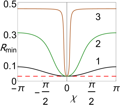
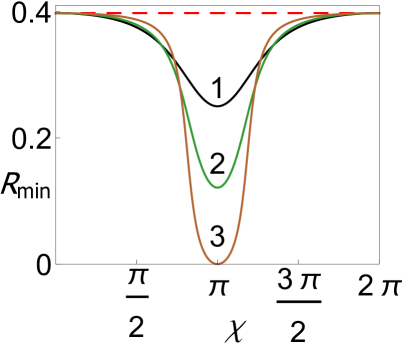
Figure 1: $R_{\text{min}}(\chi)$ for the rings closed by $0$ junction (left panel) and $\pi$ junction (right panel). Left panel: $g_{\delta}=0.1$ and    (1)  $g_{\ell}=0.1$   (2)  $g_{\ell}=0.7$   (3)  $g_{\ell}=5$,   and $g_{\ell}=0$ - dashed curve. Right panel: $g_{\delta}=3$ and    (1)  $g_{\ell}=-1$   (2)  $g_{\ell}=-1.3$   (3)  $g_{\ell}=-1.5$,   and $g_{\ell}=0$ - dashed curve.

The minimum radius $R_{\text{min}}$ as a function of the phase difference, for the thin rings closed by $0$ junctions and $\pi$ junctions, is shown in the left and right panels of Fig. 1 respectively. The minimum radius has been found above by comparing the superconducting rings with various radii at fixed $\chi$. When the Josephson coupling induces a noticeable phase dependence of $R_{\text{min}}$, the critical value $R=R_{\text{min}}(\chi)$ is not necessarily to be the minimum radius of the superconducting rings with $\chi^{\prime}\neq\chi$.

In the flux-biased rings the minimum radius actually depends on $\widetilde{\Phi}$, rather than on $\chi$. The relationship between the quantities $\chi$ and $\widetilde{\Phi}$ can be obtained by integrating the first expression for the current in (5) along the ring. Since $\oint_{{\cal C}}\mathbf{A}\cdot\xi dx=\Phi$ is the full magnetic flux penetrating the ring, one gets

$$\chi+2\pi\left(\widetilde{\Phi}-n\right)=-\,2i\int\limits_{0}^{\pi R}\dfrac{dx}{f^{2}(x)}.$$ (9)

Here $n$ is the winding number and the relation $f(x)=f(-x)$ has been used.

The integration on the right hand side in (9), taken with the solution for the order parameter, results in (24), which is valid at arbitrary ring’s size. The expression (24) is substantially simplified at $R=R_{\text{min}}(\chi)$, as shown in Appendix B Note (1):

$$\widetilde{\Phi}-n=-\dfrac{1}{2\pi}\Biggl{(}\chi+\operatorname{sgn}(g_{\ell}\sin\chi)\times\\ \arccos\frac{1+g_{b}^{2}-g^{2}_{\ell}\sin^{2}\chi}{\sqrt{\Bigl{(}1+g_{b}^{2}-g^{2}_{\ell}\sin^{2}\chi\Bigr{)}^{2}+4g_{b}^{2}g_{\ell}^{2}\sin^{2}\chi}}\Biggr{)}.$$ (10)

The relationships between the magnetic flux and the phase difference, obtained in the paper, can strongly deviate from the linear dependence $\chi=-2\pi(\widetilde{\Phi}-n)$ taking place in thick rings closed by the Josephson junction, in the absence of noticeable inductance effects Barone and Paterno (1982). Due to the Meissner effect, the supercurrent vanishes along with $v_{s}$ in the depth of a thick ring, while the order parameter remains finite. On the contrary, in thin rings the supercurrent vanishes at $R=R_{\text{min}}$ together with the order parameter, while $v_{s}$, in general, stays finite. As can be seen in (9), where the right hand side represents circulation of $v_{s}$, the superfluid velocity is responsible for the nonlinear character of the relationship (10). The integral $\int{dx}\big{/}{f^{2}(x)}$ on the right hand side of (9) diverges at the transition point. However, the integral multiplied by the supercurrent $i=g_{\ell}f^{2}_{0}\sin\chi$, remains finite even in the limit $f(x)\to 0$, in accordance with the relation $f_{0}\leq f(x)$. Both sides in (9) take zero values, along with $v_{s}$, when $\chi$ is a multiple of $\pi$. In this particular case the relation (10) acquires the familiar linear character and $|\widetilde{\Phi}|$ takes an integer or a half-integer number. For example, for $|\chi|=\pi$ (and $n=0$) one gets $|\widetilde{\Phi}|=\frac{1}{2}$. Therefore, the free energy (8) has its minimum at $\widetilde{\Phi}=0$ in the case of $0$ junction, and at $|\widetilde{\Phi}|=\frac{1}{2}$ in the case of $\pi$ junction. This agrees with the emergence of the spontaneous magnetic flux penetrating the ring closed by the $\pi$ junction Bulaevskii et al. (1977).

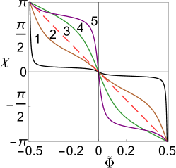
Figure 2: $\chi(\widetilde{\Phi})$ in the rings of minimum radius. $0$ junctions: $g_{\delta}=0.1$ and    (1)  $g_{\ell}=5$   (2)  $g_{\ell}=0.7$   (3)  $g_{\ell}\ll 1$.   $\pi$ junctions: $g_{\delta}=3$ and    (3)  $|g_{\ell}|\ll 1$   (4)  $g_{\ell}=-1$   (5)  $g_{\ell}=-1.5$.

The magnetic flux dependence $\chi(\widetilde{\Phi})$ in the minimum radius rings is shown in Fig. 2 for $|\widetilde{\Phi}|<0.5$, $|\chi|<\pi$. If the Josephson coupling is sufficiently weak $|g_{\ell}|\ll 1$, then the phase difference $\chi$ depends almost linearly on the magnetic flux $\widetilde{\Phi}$, as follows from (10) and seen in the dashed curve in Fig. 2. At the same time, curves 1 and 5 in Fig. 2, which correspond to $0$ and $\pi$ junctions with comparatively large Josephson coupling strengths $|g_{\ell}|$, demonstrate opposite signs of pronounced deviations from the linear behavior. Curves 1 and 5 show that the phase difference varies weakly in the wide region of $\widetilde{\Phi}$, while it undergoes abrupt changes in the narrow vicinities of the half-integer (integer) values of $\widetilde{\Phi}$ in $0$ junctions ($\pi$ junctions).

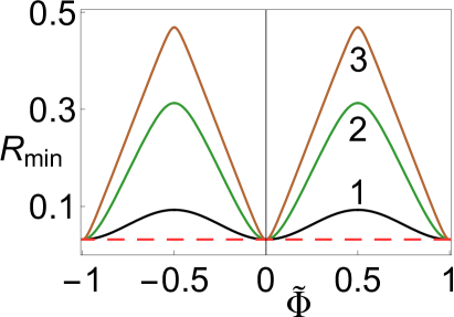
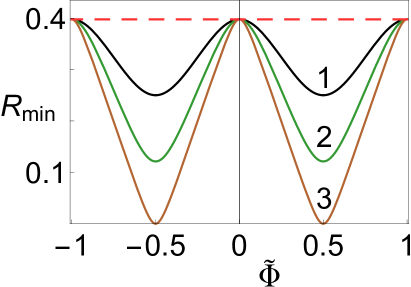
Figure 3: $R_{\text{min}}(\widetilde{\Phi})$ for the rings with $0$ junctions (left panel) and $\pi$ junctions (right panel) under the same set of parameters as in the corresponding panels in Fig. 1.

A combined consideration of (7) and (10) results in the periodic dependence of the minimum radius on the magnetic flux $R_{\text{min}}(\widetilde{\Phi})$, which is depicted in Fig. 3. The stronger the Josephson coupling strength is, the more intense the modulation of $R_{\text{min}}$ with the magnetic flux. In the case of $0$ junction ($\pi$-junction), the maxima of $R_{\text{min}}$ and of the pair breaking parameter $g_{b}$ occur at the magnetic flux half-integer (integer) values.

IV Modified critical temperature

Since temperature has been incorporated in the definitions of a number of dimensionless quantities, it implicitly enters all the results obtained above. Thus the temperature dependent coherence length $\xi(T)$, as the characteristic length of the inverse proximity effects, is included in the dimensionless radius $R(T)=r\big{/}\xi(T)$. When $R(T)$ is taken at fixed $r$, it decreases with diminishing $\tau$, and, at least formally, vanishes at $\tau=0$. Here $\tau=1-(T/T_{c0})$, and $T_{c0}$ is an unperturbed critical temperature of the superconducting material.

On the other hand, the right hand side of (7), i.e., $R_{\text{min}}$, depends on $\tau$ via the temperature dependent effective coupling constants $g_{\ell}=(g_{J}\xi(T))\big{/}K$ and $g_{\delta}=(g\xi(T))\big{/}K$. They increase with $\xi(T)$, when the temperature draws near to $T_{c}$, as a consequence of an increasing influence of the junction interface and, therefore, the boundary conditions (4), on the ring’s properties as a whole. When $\tau$ goes down, the dimensionless radius decreases down to $0$ at $\tau=0$, while the quantity $R_{\text{min}}$ increases up to $0.5$, as seen in (6) and (7).

Therefore, if the ring’s radius $R$ initially exceeds $R_{\text{min}}$ and temperature goes up, making $\xi(T)$, $g_{\ell}$ and $g_{\delta}$ sufficiently large and $\tau$ small, the quantities $R$ and $R_{\text{min}}$ will inevitably become equal to each other. The temperature $T_{c}$, at which the equality takes place, is the modified critical temperature of the superconducting transition in the ring closed by the junction. In other words, the equality $R=R_{\text{min}}$, with $R_{\text{min}}$ given in (7), can also be considered as the equation for the proximity-modified critical temperature $T_{c}<T_{c0}$ that depends on the ring’s radius and the phase difference. The critical temperature shift $\Delta T_{c}=T_{c}-T_{c0}$ is discernible within the mean field theory, when exceeding the fluctuation region near $T_{c0}$. This is the case for mesoscopic or nanoscopic rings, when the ring’s radius slightly differs from the minimum one. For a sufficiently large $R$ the shift is negligibly small.

In order to reveal the temperature dependence in the equation $R=R_{\text{min}}$, let us introduce an auxiliary ‘‘low-temperature’’ GL coherence length $\xi_{0}^{\text{GL}}=\xi(T)\sqrt{\tau}$  and move on to a rescaled dimensionless radius $\widetilde{R}=r\big{/}\xi_{0}^{\text{GL}}=R\big{/}\sqrt{\tau}$. The effective ‘‘low-temperature’’ coupling constants of the GL theory are defined as $g_{\ell 0}=(g_{J}\xi_{0}^{\text{GL}})\big{/}K$, $g_{\delta 0}=(g\xi_{0}^{\text{GL}})\big{/}K$. With these definitions, one gets from (7) the following relationship

$$\widetilde{R}\!=\dfrac{1}{2\pi\sqrt{\tau}}\arccos\dfrac{\tau-g^{2}_{\ell 0}\sin^{2}\!\chi-g^{2}_{b0}}{\sqrt{\smash[bg]{\left(\tau-g^{2}_{\ell 0}\sin^{2}\!\chi-g^{2}_{b0}\right)^{2}+4g^{2}_{b0}\tau}}}\,,$$ (11)

which can be used either as the expression for the temperature dependent minimum radius $\widetilde{R}_{\text{min}}\bigl{(}\frac{T}{T_{c0}},\chi\bigr{)}$, or as the equation for the critical temperature shift $\tau_{c}(\widetilde{R},\chi)=1-\frac{T_{c}(\widetilde{R},\chi)}{T_{c0}}=-\frac{\Delta T_{c}(\widetilde{R},\chi)}{T_{c0}}$ in the ring with radius $\widetilde{R}$.

At a given temperature, the extrema of $\widetilde{R}_{\text{min}}\bigr{(}\frac{T}{T_{c0}},\chi\bigr{)}$ take the form

$$\widetilde{R}_{\text{min}}\Bigl{(}\frac{T}{T_{c0}},\pi\Bigr{)}=\dfrac{1}{2\pi\sqrt{\tau}}\arccos\dfrac{\tau-(g_{\delta 0}+2g_{\ell 0})^{2}}{\tau+(g_{\delta 0}+2g_{\ell 0})^{2}}\,,$$ (12)

$$\widetilde{R}_{\text{min}}\Bigl{(}\frac{T}{T_{c0}},0\Bigr{)}=\dfrac{1}{2\pi\sqrt{\tau}}\arccos\dfrac{\tau-g_{\delta 0}^{2}}{\tau+g_{\delta 0}^{2}}\,.$$ (13)

The temperature dependence of the extrema of $\widetilde{R}_{\text{min}}(\chi)$ near $T_{c}$ is depicted in Fig. 4 for $0$ junctions (the left panel) and $\pi$ junctions (the right panel).

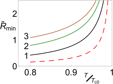
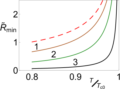
Figure 4: $\widetilde{R}_{\text{min}}(\frac{T}{T_{c0}})$ at $\chi=0,\pi$ for rings with $0$ junction (left panel) and $\pi$ junction (right panel). Left panel:  $g_{\delta 0}=0.1$,  $\chi=\pi$ and (1)  $g_{\ell 0}=0.1$   (2)  $g_{\ell 0}=0.4$   (3)  $g_{\ell 0}=5$;  $\chi=0$ - dashed curve.  Right panel:  $g_{\delta 0}=3$,  $\chi=\pi$ and (1)  $g_{\ell 0}=-1.2$   (2)  $g_{\ell 0}=-1.4$   (3)  $g_{\ell 0}=-1.48$;  $\chi=0$ - dashed curve.

For $0$ junctions, the temperature dependent minimal value $\widetilde{R}_{\text{min}}\bigr{(}\frac{T}{T_{c0}},0\bigr{)}$ is independent of $g_{\ell 0}$, being the same for $g_{\delta 0}=0.1$ and various values of $g_{\ell 0}$ considered in the left panel in Fig. 4 (the dashed curve). The solid curves in the Fig. 4 left panel demonstrate the temperature dependent maximum $\widetilde{R}_{\text{min}}\bigr{(}\frac{T}{T_{c0}},\pi\bigr{)}$ at various values of $g_{\ell 0}$ for $g_{\delta 0}=0.1$. For $\pi$ junctions, the temperature dependent maximum $\widetilde{R}_{\text{min}}\bigr{(}\frac{T}{T_{c0}},0\bigr{)}$ is independent of $g_{\ell 0}$, being the same for $g_{\delta 0}=3$ and various values of $g_{\ell 0}$ considered in the right panel of Fig. 4 (the dashed curve). The solid curves in the right panel of Fig. 4 demonstrate the temperature dependent minimum $\widetilde{R}_{\text{min}}\bigr{(}\frac{T}{T_{c0}},\pi\bigr{)}$, taken at various negative values of $g_{\ell 0}$ for $g_{\delta 0}=3$.

As seen in (11), the upper bound on the shift of the critical temperature is $\tau_{c}\leq 1/(4\widetilde{R}^{2})$. While $\xi(T)$ diverges at $T=T_{c0}$, it stays finite at $T=T_{c}<T_{c0}$. Taking jointly the upper bound obtained and the simplest condition $\tau_{c}\ll 1$ for the GL theory to be applied, one gets $4\widetilde{R}^{2}\gg 1$, which also agrees with the applicability domain of the GL theory.

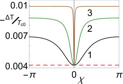
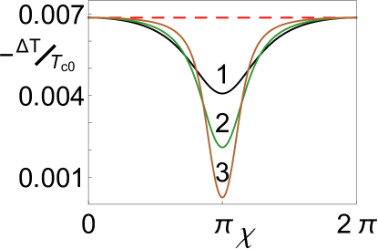
Figure 5: $-\,\frac{\Delta T_{c}}{T_{c0}}$ as a function of $\chi$ in rings with $0$ junction (left panel) and $\pi$ junction (right panel); $\widetilde{R}=5$. Left panel: $g_{\delta 0}=0.1$ and    (1)  $g_{\ell 0}=0.1$   (2)  $g_{\ell 0}=0.4$   (3)  $g_{\ell 0}=5$;   $g_{\ell 0}=0$ - dashed line. Right panel: $g_{\delta 0}=0.3$ and    (1)  $g_{\ell 0}=-0.1$   (2)  $g_{\ell 0}=-0.13$   (3)  $g_{\ell 0}=-0.148$;   $g_{\ell 0}=0$ - dashed line.

One notes, for example, that under the particular conditions $\tau_{c}\ll\min\bigl{(}1,g_{b0}^{2}+g^{2}_{\ell 0}\sin^{2}\chi\bigr{)}$, the solution of equation (11) takes the form

$$\tau_{c}(\widetilde{R},\chi)=-\dfrac{\Delta T_{c}}{T_{c0}}\approx\dfrac{\pi^{2}}{4\left(\pi\widetilde{R}+\dfrac{g_{b0}(\chi)}{g_{b0}^{2}+g^{2}_{\ell 0}\sin^{2}\chi}\right)^{2}}.$$ (14)

The critical temperature shift $\tau_{c}(\widetilde{R},\chi)$ as a function of the phase difference is shown in Fig. 5 for the rings with $\widetilde{R}=5$, closed by $0$ junction (left panel) and $\pi$ junction (right panel). For $0$ junction ($\pi$ junction) the shift takes its maxima at $\chi=(2m+1)\pi$ ($\chi=2m\pi$) and minima at $\chi=2m\pi$ ($\chi=(2m+1)\pi$).

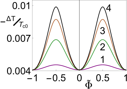
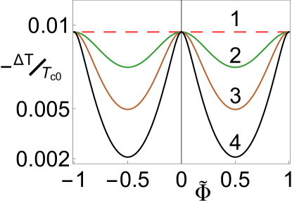
Figure 6: $-\,\frac{\Delta T_{c}}{T_{c0}}$ as a periodic function of $\widetilde{\Phi}$ in a ring with radius $\widetilde{R}=5$, closed by $0$ junction (left panel), and $\pi$ junction (right panel). Left panel: $g_{\delta 0}=0.1$ and    (1)  $g_{\ell 0}=0.01$   (2)  $g_{\ell 0}=0.1$   (3)  $g_{\ell 0}=0.4$   (4)  $g_{\ell 0}=5$. Right panel: $g_{\delta 0}=3$ and    (1)  $g_{\ell 0}=0$   (2)  $g_{\ell 0}=-1.3$   (3)  $g_{\ell 0}=-1.43$   (4)  $g_{\ell 0}=-1.48$.

The dependence of the magnetic flux $\Phi_{c}(\widetilde{R},\chi)$, taken at the modified critical temperature, can be obtained by extracting the temperature dependence in equation (10) and substituting for $\tau$ the solution of (11) $\tau_{c}(\widetilde{R},\chi)$. This allows one to get the relative shift of the critical temperature $-\,\frac{\Delta T_{c}}{T_{c0}}$ as a periodic function of the magnetic flux $\widetilde{\Phi}$, shown in Fig.  6 for $0$ junction (the left panel) and $\pi$ junction (the right panel). As expected, the shift of $T_{c}$ obtained is comparatively small but can lie beyond the fluctuation region near $T_{c}$, in a wide range of $g_{\delta 0}$ and $g_{\ell 0}$ variations.

V Radius-dependent Josephson current

A noticeable dependence of the Josephson current on the ring’s radius appears, when $r$ becomes close to the minimum radius. Since $r_{\text{min}}$ depends on the phase difference, not only the critical current, but also the current-phase relation of the junction can be strongly modified, when $r$ either exceeds the minimum radius for some of phase differences, or goes slightly over its maximum. With increasing $r$ at $r\gtrsim\xi(T)$, the current-phase relation quickly approaches the one describing the junctions included in asymptotically large rings, or in straight long superconducting leads.

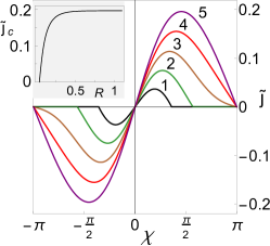
Figure 7: $\tilde{\jmath}(\chi)$ for $0$ junction: ($g_{\ell}=g_{\delta}=0.1$) included in the rings with various $R$:   (1)  $R=0.05$   (2)  $R=0.07$   (3)  $R=0.1$   (4)  $R=0.16$   (5)  $R\gg 1$. Inset: The critical current $\tilde{\jmath}_{c}$ as a function of $R$.

The normalized circulating supercurrent $\tilde{\jmath}=j/j_{\text{dp}}$ is depicted as a function of the phase difference in the main panel of Fig. 7 for various ring’s radii and for $0$ junction with $g_{\ell}=g_{\delta}=0.1$. The numerical results have been obtained by carrying out the evaluation of the supercurrent (5) with the exact self-consistent formulas of Appendix A. For the set of parameters chosen, one gets from (7) $r_{\text{min}}(0)\approx 0.0317\xi(T)$ and $r_{\text{min}}(\pi)\approx 0.093\xi(T)$. Curves 1-3 in Fig. 7 correspond to the condition $r_{\text{min}}(0)<r\lesssim r_{\text{min}}(\pi)$, while curve 5 describes the current-phase relation of the same junction included in a large ring. The dependence of the critical current on the ring’s radius is shown for the same set of parameters in the inset in Fig. 7. The critical current vanishes at $r=r_{\text{min}}(0)$, while at $r\geq\xi(T)$ its value is quite close to the asymptotic one.

The current-phase relations of $\pi$ junction with $g_{\ell}=-0.1$ and $g_{\delta}=0.3$, which closes the rings with the same set of radii, are shown in the main panel of Fig. 8. For curves 1-3 in Fig. 8, $\pi$ junction destroys superconductivity in the rings in a vicinity of $\chi=2m\pi$, while the supercurrent still survives at phase differences closer to $\chi=(2m+1)\pi$. The dependence of the critical current on the ring’s radius is similar to the case of $0$ junction. For $g_{\ell}=-0.1$ and $g_{\delta}=3$, the critical current vanishes at $r=r_{\text{min}}(\pi)\approx 0.0317\xi(T)$, while at $r\geq\xi(T)$ its value is quite close to the asymptotic one.

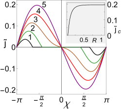
Figure 8: $\tilde{\jmath}(\chi)$ for $\pi$ junction  ($g_{\ell}=-0.1$ and $g_{\delta}=0.3$) included in the rings with various $R$:   (1)  $R=0.05$   (2)  $R=0.07$   (3)  $R=0.1$   (4)  $R=0.16$   (5)  $R\gg 1$. Inset: The critical current $\tilde{\jmath}_{c}$ as a function of $R$.

The magnetic flux dependence of the Josephson current can be found, in the case of $0$ junction, combining the phase dependence of the supercurrent shown in Fig. 7 with such a dependence of the magnetic flux given by (24). Unlike the current-phase relation, the current-magnetic flux relation in thin superconducting rings substantially depends on the radius even at large $R$. In the absence of the Meissner screening, the circulation of $v_{s}$ described on the right hand side of (9), enters and can considerably change the relation between $\Phi$ and $\chi$. As was shown in Sec. III, the circulation of $v_{s}$ noticeably modifies the $\Phi-\chi$ relation even at small $r$, i.e., quite close to the transition point $r=r_{\text{min}}$, where the superfluid velocity does not vanish. At sufficiently large $r$, which enters the upper limit of the integration in (9), the ‘‘$v_{s}$-term’’ in (9) increases $\propto r$ and has a profound influence on the $\Phi-\chi$ relation. While at small $r$ the dependence $\Phi(\chi)$ is a monotonic one within the period $2\pi$, resulting in the single valued inverse function $\chi(\Phi)$, in the rings with comparatively large radii a nonmonotonic dependence $\Phi(\chi)$ can appear and lead to a multivalued dependence of $\chi$ (and, therefore, of $j(\chi)$) on the full magnetic flux $\Phi$.

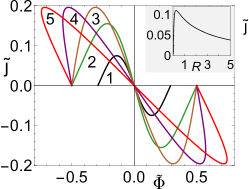
Figure 9: $\tilde{\jmath}(\widetilde{\Phi})$ in thin mesoscopic rings closed by $0$ junction with $g_{\ell}=g_{\delta}=0.1$, at various values of rings’s radii:   (1)  $R=0.07$   (2)  $R=0.16$   (3)  $R=1.03$   (4)  $R=4.00$   (5)  $R=6.50$. Inset: The supercurrent $\tilde{\jmath}$, taken at $\widetilde{\Phi}=-0.1$, as a function of the ring’s radius.

The resulting supercurrent-magnetic flux relation for $0$ junction is shown in Fig. 9. The relation between the magnetic flux and the phase difference for curves 1 and 2 is almost linear, as could be expected from discussing it in Sec. III in the case of $g_{\ell}=g_{\delta}=0.1\ll 1$ and at a sufficiently small $R$. However, the ring’s radii that correspond to curves 4 and 5, are already large enough for the $v_{s}$-term to substantially shift the magnetic flux, when the supercurrent is comparatively large. When $\chi$ is a multiple of $\pi$, the effect of the $v_{s}$-term vanishes together with $v_{s}$ and $j$. This ultimately results in the multivalued supercurrent-magnetic flux relation, as seen in curves 4 and 5. Such a behavior implies also a nonmonotonic radius dependence of the supercurrent at a fixed magnetic flux, as seen in the inset in Fig. 9.

The magnetic flux dependence of the supercurrent flowing along the rings closed by $\pi$ junction, is demonstrated in Fig. 10. Curve 1 represents the supercurrent-magnetic flux relation for the ring’s radius satisfying the conditions $R_{\text{min}}(0.5)<R<R_{\text{min}}(0)$. Superconductivity is destroyed in such a ring at small values of the full magnetic flux $\widetilde{\Phi}$, while it exists, and a finite supercurrent flows, in a vicinity of $\widetilde{\Phi}=0.5$.

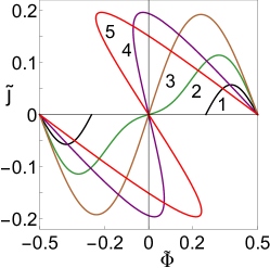
Figure 10: $\tilde{\jmath}(\widetilde{\Phi})$ in thin mesoscopic rings closed by $\pi$ junction with $g_{\ell}=-0.1$ and $g_{\delta}=0.3$, at various values of rings’s radii:   (1)  $R=0.06$   (2)  $R=0.10$   (3)  $R=0.40$   (4)  $R=4.00$   (5)  $R=6.50$.

As known, the spontaneous supercurrent and self magnetic flux arise in the superconducting rings closed by $\pi$ junction Bulaevskii et al. (1977); Sigrist and Rice (1992); Radović et al. (1999); Ariando et al. (2007). The spontaneous flux is a nontrivial solution of the equation $\Phi=\frac{1}{c}LI$, where the total supercurrent is considered as a function of the magnetic flux. Since the inductance contribution is of importance for the effect, the magnetic-field term $\frac{1}{2c^{2}}LI^{2}$ should be added to the free energy of the flux-biased ring, identified in Appendix A. A nontrivial solution is, as a rule, energetically more favorable than at $\Phi=0$. As the supercurrent vanishes at $\Phi=0.5\Phi_{0}$, for sufficiently large $L$ the solution with a comparatively small supercurrent and a flux close to half a flux quantum exists. On the contrary, there is no nontrivial solution of the equation $\Phi=\frac{1}{c}LI(\Phi)$ for sufficiently small $L$. When the difference $R-R_{\text{min}}$ diminishes, the minimum inductance for the nontrivial solution to appear increases since the superconductivity region in a vicinity of half a flux quantum, as well as the supercurrent within the region, are reduced by the inverse proximity effects (see Fig. 10). Therefore, when the effects are noticeable and the temperature draws near to $T_{c}$, the spontaneous supercurrent can disappear at sufficiently small nonzero value of $R-R_{\text{min}}$, i.e., below $T_{c}$.

Consider now the evolution of the current-magnetic flux relation with temperature. The temperature dependence of the supercurrent $j=\tilde{\jmath}j_{\text{dp}}$ originates not only from the dimensionless radius $R=\widetilde{R}\tau^{1/2}$ and from the effective coupling constants $g_{\ell\,(\delta)}=g_{\ell 0\,(\delta 0)}/\sqrt{\tau}$, but also from the temperature dependence of the depairing current $j_{\text{dp}}\propto\tau^{3/2}$. For extracting the temperature dependence of $j$, it is convenient to switch over to a new dimensionless quantity $J=j/j_{\text{dp}}^{GL}(0)$, where $j_{\text{dp}}^{GL}(0)$ is the so called zero-temperature depairing current of the GL theory $j_{\text{dp}}^{GL}(0)=\tau^{-3/2}j_{\text{dp}}$. The quantity $j_{\text{dp}}^{GL}(0)$ is known to exceed in $2-3$ times the real zero temperature depairing current $j_{\text{dp}}(0)$. For example, the equality $j_{\text{dp}}(0)\approx 0.385j_{\text{dp}}^{GL}(0)$ follows from microscopic results for the junctions, involving conventional diffusive superconductors Geers et al. (2001).

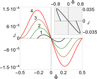
Figure 11: $J(\widetilde{\Phi})$ at $\widetilde{R}=5$,  $g_{\ell 0}=g_{\delta 0}=0.1$, taken at various temperatures:   (1)  $\tau=0.005$   (2)  $\tau=0.006$   (3)  $\tau=0.007$   (4)  $\tau=0.008$. Inset: The multivalued current-magnetic flux relation at $g_{\ell 0}=g_{\delta 0}=0.1$, $\widetilde{R}=15$ and $\tau=0.1$.

The magnetic flux dependence of $J$, taken near $T_{c}$ at various values of $\tau$, is shown in Fig. 11 for the ring with $\widetilde{R}=5$ and $g_{\ell\,(\delta),0}=0.1$. The supercurrent takes quite small values, as it is taken in units of $j_{\text{dp}}^{GL}(0)$, and not of $j_{\text{dp}}$. At substantially larger values of $\widetilde{R}$ and $J$, the multivalued current-magnetic flux relation can arise with varying temperature, and hence $\tau$, as shown in the inset for the case $\tau=0.1\ll 1$ and $\widetilde{R}=15$.

This paper has focused on the mean field results within the GL theory. The current-phase relation of the junction in the superconducting ring can also be affected both by classical fluctuations of the order parameter in or close to the fluctuation region near $T_{c}$, and by quantum fluctuations, which are of importance at very low temperatures. The former case is still an open field for further study, while a number of results have already been obtained regarding the latter one Hekking and Glazman (1997).

VI Conclusions

The problem of destructive effects of the Josephson junction on superconductivity of mesoscopic or nanoscopic rings has been solved in this paper within the GL theory. The superconducting state is shown to take place, when the ring’s radius exceeds a minimum radius $r_{\text{min}}$ that depends on the phase difference or the magnetic flux, as well as on the temperature and the effective Josephson and interface coupling constants. Depending on the junction transparency and/or the strength of the pair breaking by the junction interface, the minimum radius can become a noticeable fraction of the temperature dependent coherence length, up to $0.5\xi(T)$. The superconductor-normal metal phase transition that takes place at $r=r_{\text{min}}$, is shown to be of the second order. The magnetic flux and temperature dependence of $r_{\text{min}}$ allow an observation of the transition under slowly varying magnetic field or temperature. The minimum radius increases when the temperature draws near to $T_{c}$, resulting in the equality $r=r_{\text{min}}(T_{c})$ at the modified critical temperature.

When the ring’s radius slightly exceeds $r_{\text{min}}$, not only the critical temperature of the superconducting state, but also the current-phase and current-magnetic flux relations can be noticeably modified by the inverse proximity effects in the ring. The specific features of these characteristics have been determined both for $0$ and $\pi$ junctions, and their dependence on the ring’s radius as well as on the temperature have been obtained. A substantial evolution of the magnetic flux dependence of the Josephson current with increasing radius of thin rings has been demonstrated to persist even at large ring’s radii and result in a multivalued behavior, while the current-phase dependence stays almost unchanged at $r\gtrsim\xi(T)$, approaching the one that describes the junctions in asymptotically large rings. The identified multivaluedness of the supercurrent’s magnetic flux dependence is related to the presence of the corresponding equilibrium and metastable states, and with possible transitions between them, which result in the hysteretic behavior of the supercurrent. The hysteretic properties, however, lie outside the scope of this paper. They appear in the rings with comparatively large radii and take place irrespective of the proximity effects’ strength, while the paper mainly concerns itself with the proximity-induced effects in the rings of smaller sizes.

Currents flowing in individual nanoscopic and mesoscopic superconducting rings can be experimentally determined using a number of methods. In addition to methods based on electrical transport measurement technique employing direct electrical contacts with the system Liu et al. (2001), there also are the non-invasive ones that use micromechanical torsional magnetometers Castellanos-Beltran et al. (2013); Petković et al. (2016) or measure the ring’s susceptibility Koshnick et al. (2007); Bert et al. (2011). The present sensitivity and accuracy of the experimental techniques as well as modern technological developments for fabrication of superconducting nanorings, nanocylinders and nano-SQUIDs Liu et al. (2001); Granata and Vettoliere (2016) represent the basis for possible observations of the theoretical predictions of this paper.

Appendix A Solutions of the GL equations

The parameter ${\cal E}$, related to the first integral of the GL equation (3) and defined as

$${\cal E}=\left(\dfrac{df(x)}{dx}\right)^{2}+\dfrac{i^{2}}{f^{2}(x)}+f^{2}(x)-\dfrac{1}{2}f^{4}(x),$$ (15)

is spatially constant, when taken for the solutions $f(x)$.

Taking $x=0$ in (15) and making use of (4) and (5), one can express $\cal E$ via $f_{0}$ and the parameters of the superconducting ring closed by the junction:

$${\cal E}=\bigl{(}1+g_{b}^{2}+g_{\ell}^{2}\sin^{2}\chi\bigr{)}f_{0}^{2}-\dfrac{1}{2}f_{0}^{4}\,.$$ (16)

Eq. (15) can be also rewritten in the form

$$\left(\dfrac{df}{dx}\right)^{2}=\dfrac{1}{2f^{2}}(f^{2}-f_{+}^{2})(f^{2}-f_{d}^{2})(f^{2}-f_{-}^{2}).$$ (17)

The quantities $t_{-}=f_{-}^{2}$, $t_{d}=f_{d}^{2}$ and $t_{+}=f_{+}^{2}$ satisfy the following set of equations

$$t_{-}+t_{d}+t_{+}=2, \qquad t_{-}t_{d}t_{+}=2i^{2},$$

$$t_{d}t_{-}+t_{d}t_{+}+ t_{-}t_{+}=2{\cal E}.$$ (18)

Apart from the boundary and periodic conditions, the solution of equation (17) is characterized by three formal extrema $f_{-},\,f_{d},\,f_{+}$ with vanishing first derivatives $\frac{df}{dx}$. When the ring closed by the junction is in the equilibrium, only one of the extrema represents an actual (maximum) value of $f(x)$ in the ring, while the other two are just auxiliary quantities. Indeed, a periodic inhomogeneous solution $t(x)=f^{2}(x)$ with only a single minimum and a single maximum in the ring, should energetically be the most favorable one. The minimum $t_{0}=f_{0}^{2}$ is induced at the junction interface $x=0$ by the pair breaking effects. In contrast to the extrema described by (17) and (18), the derivative at $x=0$ is nonzero and discontinuous in accordance with the boundary conditions (4). In the equilibrium, one expects the maximum of $t(x)$ to coincide with one of the roots of the right hand side of (17) (let it be $t_{d}$), and to be realized at the point $x=\pi R$ diametrically opposed to $x=0$. In general, either all three roots $t_{-},\,t_{d}$ and $t_{+}$ take real values, or only one is real and the other two are the complex conjugate of each other. As the left hand side of (17) takes nonnegative values, one concludes that the minimum that does not actually show up in the ring (let it be $t_{-}$), has to be real in both cases. Since one of the other two extrema is the real quantity $t_{d}$, both of them also have to be real.

Let $t(x)$ have a minimum $t_{0}$ at $x=0$ and a maximum $t_{d}$ at $x=\pi R$. A nonnegative value of the left hand side of (17) entails the existence of one more maximum $t_{+}$. Assuming that $t_{-}\leq t_{0}\leq t(x)\leq t_{d}\leq t_{+}$, the solution of (17) can be represented in the region $|x|\leq\pi R$ as

$$|x|=\sqrt{\dfrac{2}{t_{+}-t_{-}}}\left[F\left(\left.\arcsin\sqrt{\dfrac{t-t_{-}}{t_{d}-t_{-}}}\right|\,\dfrac{t_{d}-t_{-}}{t_{+}-t_{-}}\right)-\right.\\ \left.-F\left(\left.\arcsin\sqrt{\dfrac{t_{0}-t_{-}}{t_{d}-t_{-}}}\right|\,\dfrac{t_{d}-t_{-}}{t_{+}-t_{-}}\right)\right].$$ (19)

Here $F\left(\varphi\left|\,m\right.\right)$ is the elliptic integral of the first kind. The notations of arguments of elliptic integrals vary in literature and here the definitions of the Mathematica book are used Wolfram (2003). Making use of the addition theorem for $F(\varphi|m)$ Prasolov and Solovyev (1997), the solution (19) can be rewritten in the form

$$|x|=\sqrt{\dfrac{2}{t_{+}-t_{-}}}F\left(\psi\left|\,\dfrac{t_{d}-t_{-}}{t_{+}-t_{-}}\right.\right),$$ (20)

where

$$\sin\psi=\dfrac{\sqrt{\left(t-t_{-}\right)\left(t_{d}-t_{0}\right)\left(t_{+}-t_{0}\right)}-\sqrt{\left(t_{0}-t_{-}\right)\left(t_{d}-t\right)\left(t_{+}-t\right)}}{\left(t_{d}-t_{-}\right)\left(t_{+}-t_{-}\right)-\left(t-t_{-}\right)\left(t_{0}-t_{-}\right)}\sqrt{t_{+}-t_{-}}\enspace.$$ (21)

The solution (20), (21) contains four parameters $t_{-}$, $t_{d}$, $t_{+}$ and $t_{0}$. They are linked to each other by the system of three equations (18), where expressions (5) and (16) should be substituted for ${\cal E}$ and $i$. The fourth equation is obtained taking $x=\pi R$ and $t(\pi R)=t_{d}$ in (20):

$$\!\pi R=\\ \!=\!\sqrt{\dfrac{2}{t_{+}-t_{-}}}F\!\left(\!\arcsin\sqrt{\dfrac{(t_{+}-t_{-})(t_{d}-t_{0})}{(t_{d}-t_{-})(t_{+}-t_{0})}}\,\left|\dfrac{t_{d}-t_{-}}{t_{+}-t_{-}}\right.\!\right).$$ (22)

When the relation (22) is taken into account, the solution (20)-(21) is simplified and can be reduced to the form

$$|x|=\pi R-\\ -\,\sqrt{\dfrac{2}{t_{+}-t_{-}}}F\biggl{(}\arcsin\sqrt{\dfrac{\left(t_{+}-t_{-}\right)\left(t_{d}-t\right)}{\left(t_{d}-t_{-}\right)\left(t_{+}-t\right)}}\,\left|\dfrac{t_{d}-t_{-}}{t_{+}-t_{-}}\right.\biggr{)},\\ |x|\leq\pi R.$$ (23)

A joint solution of (18) and (22) represents $t_{-},\,t_{0},\,t_{d}$ and $t_{+}$, as well as the whole of the inhomogeneous profile of the order parameter (23), as functions of the phase difference $\chi$ and of the dimensionless radius of the ring $R=r\big{/}\xi(T)$.

In the case of a flux-biased ring the relationship (9) between the phase difference and the magnetic flux should be used. The integration on the right hand side of (9) can be carried out after inserting the order parameter profile (23). The result contains the elliptic integral of the third kind and takes the form

$$\widetilde{\Phi}-n=-\left\{\dfrac{\chi}{2\pi}+\,i\Biggl{[}\dfrac{1}{t_{+}}R+\dfrac{\sqrt{2}\left(t_{+}-t_{d}\right)}{\pi t_{+}t_{d}\sqrt{t_{+}-t_{-}}}\,\Pi\left(\dfrac{t_{+}\left(t_{d}-t_{-}\right)}{t_{d}\left(t_{+}-t_{-}\right)};\left.\arcsin\sqrt{\dfrac{\left(t_{+}-t_{-}\right)\left(t_{d}-t_{0}\right)}{\left(t_{d}-t_{-}\right)\left(t_{+}-t_{0}\right)}}\,\right|\dfrac{t_{d}-t_{-}}{t_{+}-t_{-}}\right)\Biggr{]}\right\}\,.$$ (24)

When the solutions of (18), (22) for $t_{-}$, $t_{d}$, $t_{+}$ and $t_{0}$, along with the second expression in (5) for the supercurrent, are inserted on the right hand side of (24), the latter represents the quantity $\widetilde{\Phi}-n$ as a function of $\chi$ and $R$. As follows from (24), the magnetic flux equals an integral (a half-integral) number, when the phase difference is an even (odd) multiple of $\pi$, since the supercurrent vanishes at $\chi=m\pi$. Since the change of the winding number by one is, by definition, the change of the order-parameter phase $\phi(x)$ by $2\pi$ after it has gone around the loop, the changes of $\chi$ by a multiple of $2\pi$ and of the winding number by an integer are unambiguously interrelated in (24). The $2\pi$-periodic dependence of $t_{-}$, $t_{d}$, $t_{+}$ and $t_{0}$ on $\chi$ that follows from (18), (22) and (5), (16), should be noted here.

If the critical current is small as compared to the depairing current and the ring’s radius satisfies the condition $R\lesssim 1$, the quantity $\widetilde{\Phi}-n$ in (24), as a function of $\chi$ and $R$, can be inversed resulting in a single valued function $\chi(\widetilde{\Phi}-n,R)$. This allows one to obtain all the quantities as functions of $\widetilde{\Phi}-n$ and $R$. Similar to the unbroken rings, the dependence of the winding number on the magnetic flux should be determined from the minimization of thermodynamic potential at a fixed $\widetilde{\Phi}$. In this case one gets the physical quantities in the equilibrium state as periodic functions of $\widetilde{\Phi}$ with unit period: $\chi(\widetilde{\Phi}+1)=\chi(\widetilde{\Phi})+2\pi$.

While the superconducting state in the ring closed by the junction is inevitably inhomogeneous unless the effective coupling constants $g_{\ell}$ and $g_{\delta}$ vanish, the equilibrium state of the unbroken cylindrically symmetric thin ring is characterized by the spatially constant absolute value of the order parameter. However, an inhomogeneous profile of the order parameter can arise as an unstable (metastable) state of the uninterrupted rings Horane et al. (1996); Vodolazov et al. (2002); Castro and López (2005). Such a nonuniform solution follows from (22) - (24) in the limit $t_{0}\to t_{-}$ and $\chi\to 0$. For the unbroken rings, the three extrema $t_{-}$, $t_{d}$ and $t_{+}$ can be calculated, as functions of $\widetilde{\Phi}$ and $R$, based on the first equation in (18), as well as on (22) and (24). The inhomogeneous solution does not always exist in the unbroken axially symmetric rings, for example, at sufficiently small magnetic fluxes, since the condition $\chi\equiv 0$ makes the equation (24) to be substantially more restrictive than in the case of rings with a junction. The junction breaks the ring’s axial symmetry, that modifies the nonuniform solution and stabilizes it. Some other examples of its stabilization in rings with the broken symmetry have been discussed earlier Berger and Rubinstein (1995, 1997); Kanda et al. (2007).

The spatial integration can also be taken analytically in the expression for the bulk thermodynamic potential, with the solution (23) of the GL equation inserted in (1). As a result, one gets the free energy in the form

$$\widetilde{\cal F}=g_{b}t_{0}-\,\dfrac{\sqrt{2}}{3}\sqrt{\bigl{(}t_{+}-t_{0}\bigr{)}\bigl{(}t_{d}-t_{0}\bigr{)}\bigl{(}t_{0}-t_{-}\bigr{)}}\,-\dfrac{\pi R}{3}\Bigl{[}2t_{+}-\bigl{(}1+g_{b}^{2}+g_{\ell}^{2}\sin^{2}\chi\bigr{)}t_{0}+\dfrac{1}{2}t_{0}^{2}\Bigr{]}+\\ +\dfrac{2\sqrt{2}}{3}\biggl{[}\sqrt{t_{+}-t_{-}}\,E\Biggl{(}\left.\arcsin\sqrt{\dfrac{\left(t_{+}-t_{-}\right)\left(t_{d}-t_{0}\right)}{\left(t_{d}-t_{-}\right)\left(t_{+}-t_{0}\right)}}\,\right|\,\dfrac{t_{d}-t_{-}}{t_{+}-t_{-}}\Biggr{)}-\sqrt{\dfrac{\left(t_{d}-t_{0}\right)\left(t_{0}-t_{-}\right)}{\left(t_{+}-t_{0}\right)}}\biggr{]}\,,$$ (25)

where $\widetilde{\cal F}=(b{\cal F})\Big{/}(2K^{1/2}|a|^{3/2})$, ${\cal F}={\cal F}_{b}+{\cal F}_{\text{int}}$, and $E(\left.\varphi\,\right|m)$ is the elliptic integral of the second kind. Similar to Eq. (24) for the magnetic flux, the free energy (25) is given as a function of $\chi$ and $R$, as the quantities $t_{-}$, $t_{d}$, $t_{+}$ and $t_{0}$ are the solutions of (18) and (22).

Thermodynamic potential (25) takes into account both the bulk and the proximity-modified interface contributions. Near the transition point $R=R_{\text{min}}$ the two contributions strongly compete with each other and the result is described by formula (8) of the paper.

Since a joint solution of equations (18), (22) and (24) allows one to get the supercurrent (5) as a function of $R$ and of the full magnetic flux $\Phi$, the relation

$$\Phi_{e}=\Phi-\dfrac{1}{c}LI$$ (26)

gives in this case the applied magnetic flux $\Phi_{e}(\Phi,R)$. Here $I={\cal A}j$ is the total supercurrent, ${\cal A}$ is the cross section’s area and $L$ is the inductance. As discussed in Sec. I, the inductance effects can be safely ignored whenever $R-R_{\text{min}}$ is sufficiently small. The main focus of the paper is on a relatively small $R-R_{\text{min}}$, when the self-field effects can be mostly disregarded.

Appendix B Derivation of minimum radius

An effect of the ring’s size $R$ on the inhomogeneous solution of the GL equation is described by equation (22). Were the first argument of the elliptic integral on the right hand side of (22) arbitrarily small at a finite $t(x)$, the equation (22) would allow superconductivity in the rings with very small radii, on the scale of the GL theory. On account of the conditions $0\leq t_{-}\leq t_{0}\leq t(x)\leq t_{d}\leq t_{+}$, the first argument vanishes only at $t_{d}=t_{0}$, i.e., for the uniform order parameter. However, such a profile is incompatible with the proximity-induced boundary conditions (4) unless the effective coupling constants $g_{\ell}$, $g_{\delta}$ vanish. Indeed, substituting the equality $t_{d}=t_{0}$, as well as (5) and (16), in (18), one gets the homogeneous normal metal state, where $t_{d}=t_{0}=t_{-}=0$ and $t_{+}=2$.

In order to obtain the minimum radius $R_{\text{min}}$, one should find not only the limits of the individual extrema $t_{d},\,t_{-}$ and $t_{+}$ at the transition ($t_{0}\to 0$), but also of the combinations of these quantities, which form the arguments of the elliptic integral in (22). Small deviations from the individual limits have to be considered for this purpose. As seen in (16) and (5), both ${\cal E}$ and $i$ are the small parameters, when the minimum of $t(x)$ is small, $t_{0}\ll 1$. It is the case, when the radius of a superconducting ring only slightly exceeds the minimum radius. Up to the first order terms in ${\cal E}$ and $i$, the solutions of equations (18) are

$$t_{d\,(-)}=\dfrac{\cal E}{2}\pm\sqrt{\dfrac{{\cal E}^{2}}{4}-i^{2}},\quad t_{+}=2-{\cal E}.$$ (27)

It follows from (27), as well as from the conditions $t_{0}\leq t(x)\leq t_{d}$, that superconductivity is destroyed throughout the ring simultaneously, when the minimal value of the order parameter $f_{0}$ vanishes. The absence of an isolated phase slip center $f_{0}=0$ at $x=0$ is a direct consequence of the boundary conditions (4).

Substituting expressions (16) and (5) for $\cal E$ and $i$ in (27), one finds in the limit $t_{0}\to 0$, that the second argument of the elliptic integral in (22) vanishes while the first argument remains finite. The elliptic integral of the first kind coincides with its first argument under such conditions, so that (22) transforms into Eq. (7) for the minimum radius.

If the phase difference $\chi$ across the junction is controlled by the magnetic flux penetrating the superconducting ring, the minimum radius actually depends on $\widetilde{\Phi}$, rather than on $\chi$. The relation (24) between the quantities $\chi$ and $\widetilde{\Phi}$ substantially simplifies at $R=R_{\text{min}}(\chi)$. Taking the limit $t_{0}\to 0$ in (24), one can make the substitution $t_{0}=t_{-}=t_{d}=0$ and $t_{+}=2$ everywhere except for the extrema combinations, the calculation of which requires taking account of small deviations from the presented individual limits. On top of that, the expression (5) for the supercurrent and the relation $\Pi(n;\varphi|0)=\frac{1}{\sqrt{1-n}}\arctan\left(\sqrt{1-n}\tan\varphi\right)$ should be used. The remaining combinations of quantities $t_{d}$, $t_{0}$, and $t_{-}$ can be found in the limit $t_{0}\to 0$ using (27), (16) and (5). As a result, one obtains Eq. (10) of the paper.

References

- Tinkham (1996) M. Tinkham, Introduction to Superconductivity, 2nd ed. (McGraw-Hill, New York, 1996).
- Little and Parks (1962) W. A. Little and R. D. Parks, Phys. Rev. Lett. 9, 9 (1962).
- Parks and Little (1964) R. D. Parks and W. A. Little, Phys. Rev. 133, A97 (1964).
- de Gennes (1981) P. G. de Gennes, C. R. Acad. Sc. Paris, Série II 292, 279 (1981).
- Liu et al. (2001) Y. Liu, Y. Zadorozhny, M. M. Rosario, B. Y. Rock, P. T. Carrigan, and H. Wang, Science 294, 2332 (2001).
- Schwiete and Oreg (2010) G. Schwiete and Y. Oreg, Phys. Rev. B 82, 214514 (2010).
- Silver and Zimmerman (1967) A. H. Silver and J. E. Zimmerman, Phys. Rev. 157, 317 (1967).
- Barone and Paterno (1982) A. Barone and G. Paterno, Physics and Applications of the Josephson Effect (John Wiley&Sons, New York, 1982).
- Barash (2012) Y. S. Barash, Phys. Rev. B 85, 100503 (2012).
- Barash (2014a) Y. S. Barash, Phys. Rev. B 89, 174516 (2014a).
- Barash (2014b) Y. S. Barash, Pis’ma Zh. Eksp. Teor. Fiz. 100, 226 (2014b), [JETP Lett. 100, 205 (2014)].
- Langer and Ambegaokar (1967) J. S. Langer and V. Ambegaokar, Phys. Rev. 164, 498 (1967).
- Abrikosov (1957) A. A. Abrikosov, Zh. Eksp. Teor. Fiz. 32, 1442 (1957), [Sov. Phys. JETP 5, 1174 (1957)].
- de Gennes (1963) P. de Gennes, Physics Letters 5, 22 (1963).
- Deutscher and de Gennes (1969) G. Deutscher and P. G. de Gennes, in Superconductivity, Vol. 2, edited by R. D. Parks (Marcel Dekker, Inc., New York, 1969) p. 1005.
- Abrikosov (1988) A. A. Abrikosov, Fundamentals of the Theory of Metals (North Holland, Amsterdam, 1988).
- Ginzburg and Pitaevskii (1958) V. L. Ginzburg and L. P. Pitaevskii, Zh. Eksp. Teor. Fiz. 34, 1240 (1958), [Soviet Physics JETP 34, 858-861 (1958)].
- Zaitsev (1965) R. O. Zaitsev, Zh. Eksp. Teor. Fiz. 48, 1759 (1965), [Sov. Phys. JETP 21, 1178 (1965)].
- Andryushin et al. (1993) E. A. Andryushin, V. L. Ginzburg, and A. P. Silin, Usp. Fiz. Nauk 163, 105 (1993), [Phys-Usp 36, 854-857 (1993)].
- Note (1) Expressions (7\@@italiccorr) and (10\@@italiccorr) are slightly simplified, if the function is used instead of , while their principal values are defined within the same range . Here the function is chosen, since, for instance, in Wolfram (2003) the range is used only for , while for the range has been taken.
- Bulaevskii et al. (1977) L. N. Bulaevskii, V. V. Kuzii, and A. A. Sobyanin, Pis’ma Zh. Eksp. Teor. Fiz. 25, 314 (1977), [JETP Lett. 25, 290 (1977)].
- Note (2) For a comparison of with the Bardeen-Cooper-Schrieffer coherence length see, for example, Ref. \rev@citealpnumGolubov2001.
- Sigrist and Rice (1992) M. Sigrist and T. M. Rice, J. Phys. Soc. Jpn. 61, 4283 (1992).
- Radović et al. (1999) Z. Radović, L. Dobrosavljević-Grujić, and B. Vujičić, Phys. Rev. B 60, 6844 (1999).
- Ariando et al. (2007) Ariando, H. J. H. Smilde, C. J. M. Verwijs, G. Rijnders, D. H. A. Blank, H. Rogalla, J. R. Kirtley, C. C. Tsuei, and H. Hilgenkamp, in Electron Correlation in New Materials and Nanosystems, Nato Science Series II, Vol. 241, edited by K. Scharnberg and S. Kruchinin (Springer, Dordrecht, 2007) pp. 149–174.
- Geers et al. (2001) J. M. E. Geers, M. B. S. Hesselberth, J. Aarts, and A. A. Golubov, Phys. Rev. B 64, 094506 (2001).
- Hekking and Glazman (1997) F. W. J. Hekking and L. I. Glazman, Phys. Rev. B 55, 6551 (1997).
- Castellanos-Beltran et al. (2013) M. A. Castellanos-Beltran, D. Q. Ngo, W. E. Shanks, A. B. Jayich, and J. G. E. Harris, Phys. Rev. Lett. 110, 156801 (2013).
- Petković et al. (2016) I. Petković, A. Lollo, L. I. Glazman, and J. Harris, Nature Communications 7, 13551 (2016).
- Koshnick et al. (2007) N. C. Koshnick, H. Bluhm, M. E. Huber, and K. A. Moler, Science 318, 1440 (2007).
- Bert et al. (2011) J. A. Bert, N. C. Koshnick, H. Bluhm, and K. A. Moler, Phys. Rev. B 84, 134523 (2011).
- Granata and Vettoliere (2016) C. Granata and A. Vettoliere, Physics Reports 614, 1 (2016).
- Wolfram (2003) S. Wolfram, The Mathematica Book, 5th ed. (Wolfram Media, New York, 2003).
- Prasolov and Solovyev (1997) V. Prasolov and Y. Solovyev, Elliptic Functions and Elliptic Integrals (American Mathematical Society, Providence, Rhode Island, 1997).
- Horane et al. (1996) E. M. Horane, J. I. Castro, G. C. Buscaglia, and A. López, Phys. Rev. B 53, 9296 (1996).
- Vodolazov et al. (2002) D. Y. Vodolazov, B. J. Baelus, and F. M. Peeters, Phys. Rev. B 66, 054531 (2002).
- Castro and López (2005) J. I. Castro and A. López, Phys. Rev. B 72, 224507 (2005).
- Note (3) In more involved cases one should also take in this limit ,\tmspace+.1667em and , where .
- Berger and Rubinstein (1995) J. Berger and J. Rubinstein, Phys. Rev. Lett. 75, 320 (1995).
- Berger and Rubinstein (1997) J. Berger and J. Rubinstein, Phys. Rev. B 56, 5124 (1997).
- Kanda et al. (2007) A. Kanda, B. J. Baelus, D. Y. Vodolazov, J. Berger, R. Furugen, Y. Ootuka, and F. M. Peeters, Phys. Rev. B 76, 094519 (2007).