On the correspondence between classical geometric phase of gyro-motion and quantum Berry phase

Abstract

We show that the geometric phase of the gyro-motion of a classical charged particle in a uniform time-dependent magnetic field described by Newton’s equation can be derived from a coherent Berry phase for the coherent states of the Schrödinger equation or the Dirac equation. This correspondence is established by constructing coherent states for a particle using the energy eigenstates on the Landau levels and proving that the coherent states can maintain their status of coherent states during the slow varying of the magnetic field. It is discovered that orbital Berry phases of the eigenstates interfere coherently to produce an observable effect (which we termed “coherent Berry phase”), which is exactly the geometric phase of the classical gyro-motion. This technique works for particles with and without spin. For particles with spin, on each of the eigenstates that makes up the coherent states, the Berry phase consists of two parts that can be identified as those due to the orbital and the spin motion. It is the orbital Berry phases that interfere coherently to produce a coherent Berry phase corresponding to the classical geometric phase of the gyro-motion. The spin Berry phases of the eigenstates, on the other hand, remain to be quantum phase factors for the coherent states and have no classical counterpart.

I Introduction

Berry phase Berry1984 of a quantum system is an important physical effect that has been discussed in depth Berry1985 ; Simon1983 ; AA1987 . Because Berry phase, as a quantum phase in the wave function, depends only on the geometric path of the system, it is also called geometric phase. The phenomena of geometric phase also exist in classical systems, known as the Hannay angle Hannay1985 . Geometric phase also exists in many systems in plasma physics Bhattacharjee1992 ; Liu11 ; Liu12 ; Burby13 ; Lan16 . To avoid confusion, geometric phase is used only for classical systems in this paper.

In a magnetized plasma, charged particles gyrate in the plane perpendicular to the magnetic field, exerting helical orbits. This gyro-motion of a charged particle can be characterized by a dynamic gyro-phase around the magnetic field. In a strongly magnetized plasma, the fast gyro-motion of charged particles leads to the temporal and spatial scale separation, and is usually averaged out in the magneto-hydrodynamic and traditional gyro-kinetic theories. However, the gyro-phase itself still carries important information and plays an important role in modern gyro-kinetic theories Qin00 ; Qin2007 ; Yu09 ; Burby12 . Recently, Liu and Qin Liu11 discussed the gyro-motion of a charged particle in a spatially uniform, time-dependent magnetic field Qin06 . It was found that when the magnetic field returns to its original direction, apart from the phase advance produced by the gyro-motion, there is an additional geometric phase in the gyro-phase, which equals to the solid angle $\Omega$ spanned by the trace of the magnetic field unit vector $\boldsymbol{b}$ on the unit sphere $S^{2}$. On the other hand, it is well known that the Berry phase associated with an electron spin eigenstate under the same change of the magnetic field is $\pm\frac{1}{2}\Omega$ Berry1984 , whose sign depends on the spin direction. Ref. Liu11 discussed the similarities and differences between the geometric phase in a charged particle’s gyro-motion and the Berry phase for the electron spin in quantum mechanics. However, no direct connection was found in their paper. Even though the gyro-motion is not the classical counterpart of the quantum spin, the similarities in these two geometric phases may still imply certain connections in a deeper level.

In this paper, we show a direct correspondence between the classical geometric phase of the gyro-motion and the Berry phase of the underlying quantum system, based on the use of coherent states from the Schrödinger equation. The Berry phases come from the orbital angular momentum eigenstates on the Landau levels Landau1930 , rather than the spin eigenstates. The Berry phase is governed by the Schrödinger equation, while the geometric phase of the gyro-motion is governed by Newton’s equation. The connection between the two reveals the identical physical and geometric nature for the two phases. Historically, the problem being studied here is about the quantum-classical correspondence. Berry studied the correspondence between Berry phase and Hannay angle from the semi-classical point of view Berry1985 , while the idea of using coherent state to establish such correspondence in a 1-dimensional non-degenerate system was first developed by Maamache et al Maamache90 . Here we study the correspondence problem for a 2-dimensional degenerate system in the context of charged particle dynamics in an external magnetic field.

The correspondence is establish through three steps. First, we construct a coherent state to represent the gyro-motion of a charged particle in a uniform time-independent magnetic field. Then we calculate the Berry phase for each component that makes up the coherent state during the slowly varying of the magnetic field. Lastly, we prove that the interference of these components after gaining their Berry phases results in an additional phase that naturally enters the complex variable that is used to define the coherent state. We termed this additional phase “coherent Berry phase”, which turns out to be exactly the classical geometric phase of the gyro-motion. To further clarify the relationship between the geometric phase of the gyro-motion and the Berry phase of a charged particle with spin, we will also analyze electrons with spin governed by the Dirac equation and show that the Berry phase of an eigenstate in the non-relativistic limit consists of two parts, the orbital part and the spin part. The orbital Berry phases of the eigenstates interfere coherently to produce a coherent Berry phase corresponding to the classical geometric phase of gyro-motion, while the spin Berry phases have no classical counterparts, as expected.

The term “coherent Berry phase” in this paper has not been used before. It is not an overall phase factor multiplying the wave function, but the argument $\gamma_{C}$ that enters the complex variable $w_{0}(T)$ which is used to define a coherent state. It is an observable effect resulting from the coherent interference of all the eigenstates that constitute the coherent state, each of them having gained a Berry phase $\gamma_{n}=n\gamma_{C}$ (See Sec. IV for detailed discussions). We want to distinguish it from the concept of “Berry phase of a coherent state”, which is indeed an overall phase factor in front of the coherent state, and was calculated, for example, in Ref. Yang07 ; Chaturvedi87 .

The paper is organized as follows. In Sec. II we briefly review the derivation of the geometric phase of a charged particle’s gyro-motion. We review in Sec. III the derivation of the Landau levels and construct coherent states for a charged particle in a uniform time-independent magnetic field. The Berry phase associated with a coherent state is calculated and the correspondence between the geometric phase of the gyro-motion is established in Sec. IV. In Sec. V, we calculate the Berry phases of an electron described by the Dirac equation and analyze the Berry phases due to orbital and spin degrees of freedom.

II Classical geometric phase of a charged particle’s gyro-motion

In this section, we review the derivation Liu11 of the classical geometric phase of the gyro-motion for a classical charged particle in a time-dependent magnetic field. Consider a classical charged particle with charge $q$ and mass $\mu$ in a spatially-uniform but time-dependent magnetic field $\boldsymbol{B}=B(t)\boldsymbol{b}(t)$. Newton’s equation for the particle is

$$\frac{d\boldsymbol{v}}{dt}=\omega_{d}\boldsymbol{v}\times\boldsymbol{b},$$ (1)

where $\omega_{d}(t)=qB(t)/\mu$ is the gyro-frequency. To define the gyro-phase, we need to select a frame. Choose two unit vectors $\boldsymbol{e}_{1}$ and $\boldsymbol{e}_{2}$ perpendicular to $\boldsymbol{b}$ for every possible $\boldsymbol{b}$ such that $\boldsymbol{e}_{1}\cdot\boldsymbol{e}_{2}=0$ and $\boldsymbol{e}_{1}\times\boldsymbol{e}_{2}=\boldsymbol{b}$. Note that there is a freedom in choosing $(\boldsymbol{e}_{1},\boldsymbol{e}_{2})$. Particle velocity can be decomposed in the frame $(\boldsymbol{e}_{1},\boldsymbol{e}_{2},\boldsymbol{b})$ as

$$\boldsymbol{v}=v_{\parallel}\boldsymbol{b}+v_{\perp}\cos\theta\boldsymbol{e}_{1}+v_{\perp}\sin\theta\boldsymbol{e}_{2},$$ (2)

where $\theta$ is the gyro-phase. Following Ref. Liu11 , the dynamic equation for $\theta$ is

$$\frac{d\theta}{dt}=-\left[\omega_{d}(t)+\omega_{g}(t)+\omega_{a}(t)\right],$$ (3)

$$\omega_{g}(t)=\frac{d\boldsymbol{e}_{1}}{dt}\cdot\boldsymbol{e}_{2},$$ (4)

$$\omega_{a}(t)=\frac{v_{\parallel}}{v_{\perp}}\frac{d\boldsymbol{b}}{dt}\cdot(\cos\theta\boldsymbol{e}_{2}-\sin\theta\boldsymbol{e}_{1}),$$ (5)

where $\omega_{d}(t)$ is the dynamic contribution due to gyro-motion, $\omega_{g}(t)$ is the geometric contribution, and $\omega_{a}(t)$ is the adiabatic contribution for reasons soon to be clear. The negative sign on the right-hand side of Eq. (3) is due the choice of coordinate. Liu and Qin Liu11 proved that if the magnetic field changes slowly, i.e.,

$$|\frac{1}{\omega_{d}B}\frac{d\boldsymbol{B}}{dt}|\sim\epsilon\ll 1,$$

$$|\frac{1}{\omega_{d}^{2}B}\frac{d^{2}\boldsymbol{B}}{dt^{2}}|\sim\epsilon^{2}\ll 1,$$ (6)

then the phase advances due to the dynamic, the geometric, and the adiabatic phase satisfy the following ordering,

$$\Delta\theta_{d}:\Delta\theta_{g}:\Delta\theta_{a}\sim 1:\epsilon:\epsilon^{2},$$

$$\Delta\theta_{d}\equiv-\int_{0}^{T}\omega_{d}dt,$$

$$\Delta\theta_{g}\equiv-\int_{0}^{T}\omega_{d}dt,$$

$$\Delta\theta_{a}\equiv-\int_{0}^{T}\omega_{a}dt.$$

For a slowing evolving system, the leading order correction to the dynamic phase $\Delta\theta_{d}$ is the geometric phase $\Delta\theta_{g}$. Assume that the system starts evolving from $t=0$, and at $t=T$ the magnetic field returns to its original position, i.e., $\boldsymbol{b}(T)=\boldsymbol{b}(0)$. The fact that the frame $(\boldsymbol{e}_{1},\boldsymbol{e}_{2},\boldsymbol{b})$ is defined in a single-valued manner implies that $\boldsymbol{e}_{1}(T)=\boldsymbol{e}_{1}(0)$ and $\boldsymbol{e}_{2}(T)=\boldsymbol{e}_{2}(0)$. The trace of $\boldsymbol{b}(t)$ during the time forms a closed loop $C$ on $S^{2}$. The geometric phase is calculated to be

$$\Delta\theta_{g}=-\int_{0}^{T}\omega_{g}dt=-\oint_{C}d\boldsymbol{e}_{1}\cdot\boldsymbol{e}_{2}.$$ (7)

The last integration is along the closed loop $C$ on $S^{2}$. In the spherical coordinates $(\zeta,\phi)$ with $\boldsymbol{b}=(\sin\zeta\cos\phi,\sin\zeta\sin\phi,\cos\zeta)$, we can choose $\boldsymbol{e}_{1}=(\cos\zeta\cos\phi,\cos\zeta\sin\phi,-\sin\zeta)$ and $\boldsymbol{e}_{2}=(-\sin\phi,\cos\phi,0)$. The geometric phase becomes

$$\Delta\theta_{g}=-\oint_{C}\cos\zeta d\phi=-\Omega,$$ (8)

where $\Omega$ is the solid angle expanded by $C$. We note that $\Omega$ does not depend on the choice of frame. For a different frame $(\boldsymbol{e}_{1}^{\prime},\boldsymbol{e}_{2}^{\prime},\boldsymbol{b})$ specified by a coordinate transformation

$$\begin{cases}\boldsymbol{e}_{1}^{\prime}&=\cos\psi\boldsymbol{e}_{1}+\sin\psi\boldsymbol{e}_{2},\\ \boldsymbol{e}_{2}^{\prime}&=-\sin\psi\boldsymbol{e}_{1}+\cos\psi\boldsymbol{e}_{2},\end{cases}$$ (9)

we have $d\boldsymbol{e}_{1}^{\prime}\cdot\boldsymbol{e}_{2}^{\prime}=d\boldsymbol{e}_{1}\cdot\boldsymbol{e}_{2}+d\psi$. For $\boldsymbol{b}(T)=\boldsymbol{b}(0)$, $\psi(T)=\psi(0)$ and thus $\oint d\psi=0$. Therefore, the geometric phase is unique when the magnetic field returns to its original direction.

III Landau levels and coherent states for spinless particles

In this section, we construct coherent states of a spinless charged particle in a uniform magnetic field described by the Schrödinger equation. The energy eigenstates are infinitely degenerate in each of the energy levels which are known as Landau levels Landau1930 . From these eigenstates, we can construct a coherent state which is a non-diffusive wave packet gyrating around the magnetic field and corresponds to a classical charged particle. Several authors have discussed how to construct coherent states Malkin1969 ; Feldman1970 ; Kowalsk2005 ; Murayama ; Shankar94 . Here we review these results using the notation of Refs. Murayama ; Shankar94 . It’s assumed that the particle has positive charge $q>0$ . For negative charge, the definitions will be modified accordingly, as will be seen in Sec. V.

The Hamiltonian for the charged particle of charge $q$ and mass $\mu$ in a uniform magnetic field $\boldsymbol{B}=B_{0}\boldsymbol{e}_{z}$ is

$$H=\frac{(\boldsymbol{P}-q\boldsymbol{A})^{2}}{2\mu},$$ (10)

where $\boldsymbol{P}=-i\hbar\nabla$ is the canonical momentum operator, and $\boldsymbol{A}$ is the magnetic vector potential satisfying $\nabla\times\boldsymbol{A}=\boldsymbol{B}.$ The kinetic momentum operator is $\boldsymbol{\pi}=\boldsymbol{P}-q\boldsymbol{A}$, whose $x$ and $y$-components satisfy the commutation relation

$$[\pi_{x},\pi_{y}]=i\hbar q(\partial_{x}A_{y}-\partial_{y}A_{x})=i\hbar qB_{0}.$$ (11)

We can then define creating and annihilating operators $a^{\dagger}$ and $a$ as

$$\begin{cases}a^{\dagger}=\sqrt{\frac{1}{2\hbar qB_{0}}}(\pi_{x}-i\pi_{y}),\\ a=\sqrt{\frac{1}{2\hbar qB_{0}}}(\pi_{x}+i\pi_{y}),\end{cases}$$ (12)

and prove the commutation relation $[a,a^{\dagger}]=1$.

The Hamiltonian can be written as

$$H=\hbar\omega_{d}(a^{\dagger}a+\frac{1}{2}),$$ (13)

where $\omega_{d}=qB/\mu$. Since a particle moves freely along the magnetic field, the parallel motion $\boldsymbol{P}_{z}^{2}/2\mu$ is not included for the moment (the discussion on $\boldsymbol{P}_{z}$ can be found in the Appendix). The Hamiltonian is in the same form as that of a 1D simple harmonic oscillator. Choosing $\boldsymbol{A}$ to be the rotationally symmetric form $\boldsymbol{A}=(-\frac{1}{2}B_{0}y,\frac{1}{2}B_{0}x,0)$, and using complex variables $w\equiv x+iy,$ we express the creating and annihilating operators as

$$\begin{cases}a^{\dagger}=-i\sqrt{\frac{\hbar}{2qB_{0}}}(2\partial_{w}-\frac{qB_{0}}{2\hbar}\bar{w}),\\ a=-i\sqrt{\frac{\hbar}{2qB_{0}}}(2\partial_{\bar{w}}+\frac{qB_{0}}{2\hbar}w).\end{cases}$$ (14)

Here, $\partial_{w}=\frac{1}{2}(\partial_{x}-i\partial_{y})$, $\partial_{\overline{w}}=\frac{1}{2}(\partial_{x}+i\partial_{y})$, and $w$ and $\overline{w}$ are treated as independent variables (the over-bar means complex conjugate). The ground state $\psi(w,\bar{w})$ is obtained by solving $a\psi=0$, i.e.,

$$-i\sqrt{\frac{\hbar}{2qB_{0}}}(2\partial_{\bar{w}}+\frac{qB_{0}}{2\hbar}w)\psi(w,\bar{w})=0.$$ (15)

The solution is $\psi(w,\bar{w})=g(w)e^{-qB_{0}w\bar{w}/4\hbar}$, where $g(w)$ is an arbitrary analytical function. The arbitrariness of $g(w)$ indicates the infinite degeneracy of the ground states. With the choice of $g(w)=w^{m},\,m=0,1,2,...$, a set of ground states can be obtained,

$$\psi_{0,m}=N_{m}w^{m}e^{-qB_{0}w\bar{w}/4\hbar},$$ (16)

$$N_{m}=\left[\pi m!\left(\frac{2\hbar}{qB_{0}}\right)^{m+1}\right]^{-\frac{1}{2}},$$ (17)

where $N_{m}$ is the normalization factor. Excited states are obtained using the creating operator,

$$\psi_{n,m}=\frac{(a^{\dagger})^{n}}{\sqrt{n!}}\psi_{0,m}.$$ (18)

It is easy to verify that $H\psi_{n,m}=\hbar\omega_{d}(n+\frac{1}{2})$. The eigenstates $\psi_{n,m}$ covers all the Landau levels, with each $n$ representing an energy level $E_{n}=\hbar\omega_{d}(n+\frac{1}{2})$ with infinite degeneracy. They are all the eigenstates of the angular momentum operator $\boldsymbol{L}_{z}=-i\hbar\partial_{\theta}$. In the polar coordinates with $w=\rho e^{i\theta}$, it is straightforward to show that $\psi_{n.m}\propto e^{-i(n-m)\theta}$ and that they are orthogonal to each other, i.e., $\left<\psi_{n,m}|\psi_{n^{\prime},m^{\prime}}\right>=0$, for any $(n^{\prime},m^{\prime})\neq(n,m)$.

Since the motion perpendicular to the magnetic field is essentially 4-dimensional in phase space ($x,y,\pi_{x},\pi_{y}$), one pair of creating and annihilating operators $(a^{\dagger},a)$ is incomplete. Indeed, there exists another pair of creating and annihilating operators ($b^{\dagger},b)$, defined as

$$\begin{cases}b^{\dagger}=\sqrt{\frac{qB_{0}}{2\hbar}}(X-iY),\\ b=\sqrt{\frac{qB_{0}}{2\hbar}}(X+iY),\end{cases}$$ (19)

where $(X,Y)=(x+\pi_{y}/\mu\omega_{d},y-\pi_{x}/\mu\omega_{d})$ is the guiding center position operator. Using the complex variable $w\equiv x+iy$, we have

$$\begin{cases}b^{\dagger}=\sqrt{\frac{\hbar}{2qB_{0}}}(-2\partial_{\bar{w}}+\frac{qB_{0}}{2\hbar}w),\\ b=\sqrt{\frac{\hbar}{2qB_{0}}}(2\partial_{w}+\frac{qB_{0}}{2\hbar}\bar{w}).\end{cases}$$ (20)

It can be verified that $[b,a]=[b,a^{\dagger}]=[b^{\dagger},a]=[b^{\dagger},a^{\dagger}]=0$, thus $[b,H]=[b^{\dagger},H]=0$. Also, the degenerate eigenstates on each Landau level is related by $b^{\dagger}$ and $b$,

$$\psi_{n,m}=\frac{(b^{\dagger})^{m}}{\sqrt{m!}}\psi_{n,0}.$$ (21)

Thus two pairs of creating and annihilating operators $(a^{\dagger},a)$ and $(b^{\dagger},b)$ give the complete description of motion perpendicular to the magnetic field.

A coherent state is constructed in a way similar to that of a simple harmonic oscillator. Let $f=-i\sqrt{qB_{0}/2\hbar}w_{0}$ and $R=\sqrt{qB_{0}/2\hbar}r_{0}$ where $w_{0}$ and $r_{0}$ are complex variables, a coherent state is

$$\Psi_{w_{0},r_{0}}=e^{-\frac{|f|^{2}+|R|^{2}}{2}}e^{fa^{\dagger}+Rb^{\dagger}}\psi_{0,0}$$

$$=e^{-\frac{qB_{0}}{4\hbar}w_{0}\bar{w_{0}}}e^{-\frac{w_{0}}{2}(2\partial_{w}-\frac{qB_{0}}{2\hbar}\bar{w})}\left[e^{\frac{r_{0}}{2}(-2\partial_{\bar{w}}+\frac{qB_{0}}{2\hbar}w)}(N_{0}e^{-\frac{qB_{0}w\bar{w}}{4\hbar}})\right]$$

$$=N_{0}e^{-\frac{qB_{0}}{4\hbar}(|w|^{2}+|w_{0}|^{2}+|r_{0}|^{2}+2r_{0}w_{0}-2r_{0}w-2w_{0}w)}.$$ (22)

The probability distribution of $\Psi_{w_{0},r_{0}}$ is

$$|\Psi_{w_{0},r_{0}}|^{2}=|N_{0}|^{2}e^{-\frac{qB_{0}}{2\hbar}(w-\bar{r_{0}}-w_{0})(\bar{w}-r_{0}-\bar{w}_{0})},$$ (23)

which describes a Gaussian wave packet in the $x$-$y$ plane. It centers at $w\equiv x+iy=\bar{r_{0}}+w_{0}$ and has a characteristic width $\delta=\sqrt{\hbar/qB_{0}}$. To obtain the time evolution of $\Psi_{w_{0},r_{0}}$, we decompose it into eigenstates on the Landau levels,

$$\Psi_{w_{0},r_{0}}=e^{-\frac{|f|^{2}+|R|^{2}}{2}}e^{fa^{\dagger}+Rb^{\dagger}}\psi_{0,0}=e^{-\frac{|f|^{2}+|R|^{2}}{2}}\sum_{n=0}^{+\infty}\sum_{m=0}^{+\infty}\frac{f^{n}}{\sqrt{n!}}\frac{R^{m}}{\sqrt{m!}}\psi_{n,m}.$$ (24)

The coherent state evolves according to how each eigenstates evolves,

$$\Psi_{w_{0},r_{0}}(t) =e^{-\frac{|f|^{2}+|R|^{2}}{2}}\sum_{n=0}^{+\infty}\sum_{m=0}^{+\infty}\frac{f^{n}}{\sqrt{n!}}\frac{R^{m}}{\sqrt{m!}}\psi_{n,m}e^{iE_{n}(t)}.$$

$$=e^{-\frac{|f|^{2}+|R|^{2}}{2}}\sum_{n=0}^{+\infty}\sum_{m=0}^{+\infty}\frac{f^{n}}{\sqrt{n!}}\frac{R^{m}}{\sqrt{m!}}\psi_{n,m}e^{-i\omega_{d}(n+\frac{1}{2})t}$$

$$=e^{-\frac{i\omega_{d}t}{2}}e^{-\frac{|f(t)|^{2}+|R|^{2}}{2}}\sum_{n=0}^{+\infty}\sum_{m=0}^{+\infty}\frac{[f(t)]^{n}}{\sqrt{n!}}\frac{R^{m}}{\sqrt{m!}}\psi_{n,m}$$

$$=e^{-\frac{i\omega_{d}t}{2}}\Psi_{w_{0}(t),r_{0}},$$ (25)

where $f(t)=-i\sqrt{qB_{0}/2\hbar}w_{0}(t)$ and $w_{0}(t)=w_{0}e^{-i\omega_{d}t}$. We see that $\Psi_{w_{0},r_{0}}(t)$ still describes a Gaussian wave packet, but its center has moved to $w=\bar{r_{0}}+w_{0}e^{-i\omega_{d}t}$. The coherent state $\Psi_{w_{0},r_{0}}(t)$ does not diffuse, thus represents the gyro-motion of a charged particle in a uniform time-independent magnetic field, with guiding center at $\bar{r_{0}}$, gyro-frequency $\omega_{d}$ and gyro-radius $\rho_{d}=|w_{0}|$. $w_{0}$ and $r_{0}$ are two complex variables, which have four degrees of freedom, thus will give a complete description of all the coherent states. An illustration of the coherent state described by Eq. (25) is shown in Fig. 1.

Because the magnetic field is spatially homogeneous, the system has translational invariance perpendicular to the magnetic field. Thus we can perform a coordinate transformation to move the guiding center to the origin. This coordinate transformation is accompanied by a gauge transformation to make the vector potential $\boldsymbol{A}$ rotationally invariant around the new origin. Such a gauge transformation is

$$\boldsymbol{A} \rightarrow\boldsymbol{A}-\nabla\chi,$$ (26)

$$\Psi_{w_{0},r_{0}} \rightarrow e^{-\frac{iq}{\hbar c}\chi}\Psi_{w_{0},r_{0}},$$ (27)

$$\chi(x,y) =\frac{B_{0}}{2}\left[Re(\bar{r_{0}})y-Im(\bar{r_{0}})x\right].$$ (28)

It’s found that after the gauge transformation, the wave function of the coherent state becomes

$$e^{-\frac{iq}{\hbar c}\chi}\Psi_{w_{0},r_{0}}=N_{0}e^{-\frac{qB_{0}}{4\hbar}[|w-\bar{r_{0}}|^{2}-2w_{0}(w-\bar{r_{0}})+|w_{0}|^{2}]}.$$ (29)

Thus a coordinate transformation $w\rightarrow w-\bar{r_{0}}$ will transform the wave function into

$$N_{0}e^{-\frac{qB_{0}}{4\hbar}[|w|^{2}-2w_{0}w+|w_{0}|^{2}]}=\Psi_{w_{0},0}.$$ (30)

Hence, the time-evolution of the coherent state does not depend on $r_{0}$ once we perform a gauge transformation and a coordinate transformation. In the following discussion we choose $r_{0}=0$ for simplicity, and the coherent state can be simplified to

$$\Psi_{w_{0}}\equiv\Psi_{w_{0},0}=e^{-\frac{|f|^{2}}{2}}\sum_{n=0}^{+\infty}\frac{f^{n}}{\sqrt{n!}}\psi_{n,0}.$$ (31)

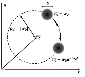
Figure 1: Illustration of the coherent state described by Eq. (25).

IV The Berry phase associated with coherent states for spinless particles

We show in this section that a coherent Berry phase can be naturally defined for the coherent states when the magnetic field evolves slowly with time, and this coherent Berry phase is exactly the geometric phase for the classical gyro-motion. We assume for simplicity that the magnitude of the magnetic field does not change, and only the field direction changes, i.e., $\boldsymbol{B}(t)=B_{0}\boldsymbol{b}(t)$. At $t=T$, the magnetic field returns to its original state, i.e. $\boldsymbol{b}(T)=\boldsymbol{b}(0)=\boldsymbol{e}_{z}$. Then the trajectory of $\boldsymbol{b}(t)$ on $S^{2}$ forms a closed loop $C$. As in Sec. II, for each $\boldsymbol{b}(t)$, we choose unit vectors $\boldsymbol{e}_{1}$ and $\boldsymbol{e}_{2}$ such that $\boldsymbol{e}_{1}\cdot\boldsymbol{e}_{2}=0$ and $\boldsymbol{e}_{1}\times\boldsymbol{e}_{2}=\boldsymbol{b}$. The Hamiltonian depends on $\boldsymbol{b}(t)$ parametrically. For a given $\boldsymbol{b}$,

$$H[\boldsymbol{b}] =\frac{\left(\boldsymbol{P}-q\boldsymbol{A}[\boldsymbol{b}]\right)^{2}}{2\mu},$$ (32)

$$\boldsymbol{A}[\boldsymbol{b}] =-\frac{1}{2}B_{0}\boldsymbol{r}\times\boldsymbol{b},$$ (33)

where $\boldsymbol{r}=(x,y,z)$ is the coordinate vector in the Cartesian frame of $\mathbb{R}^{3}$, and $\boldsymbol{P}=-i\hbar\nabla$. The eigenstates of $H[\boldsymbol{b}]$ are $\psi_{n,m}[\boldsymbol{b}]=\psi_{n,m}\left(w[\boldsymbol{b}],\bar{w}[\boldsymbol{b}]\right)$, where $w[\boldsymbol{b}]=\rho[\boldsymbol{b}]e^{i\theta[\boldsymbol{b}]}$, $\bar{w}[\boldsymbol{b}]=\rho[\boldsymbol{b}]e^{-i\theta[\boldsymbol{b}]}$ and

$$\rho[\boldsymbol{b}] =\sqrt{|\boldsymbol{r}|^{2}-[\boldsymbol{r}\cdot\boldsymbol{b}]},$$ (34)

$$\theta[\boldsymbol{\boldsymbol{b}}] =\arccos\frac{[\boldsymbol{r}-(\boldsymbol{r}\cdot\boldsymbol{b})\boldsymbol{b}]\cdot\boldsymbol{e}_{1}}{\rho[\boldsymbol{b}]}.$$ (35)

In the above equations, the notation $[\boldsymbol{b}]$ denotes the parametric dependence on $\boldsymbol{b}$. For example, $\psi_{n,m}[\boldsymbol{b}(t)]$ is an eigenstate corresponding to the $\boldsymbol{b}$ at the instant of $t$. It is not the solution of the time-dependent Schrödinger equation.

Now the question is, if the system is at a coherent state $\Psi_{w_{0}}$ at $t=0$, what is the state of the system at $t=T$ under a slow evolution of $\boldsymbol{b}(t)$? To answer this question, we first look at how each eigenstate evolves. According to the well-known adiabatic theorem Messiah1962 , it is expected that each eigenstate $\psi_{n,0}(t=0)$ is evolved into the eigenstate $\psi_{n,0}[\boldsymbol{b}(t)]$. However, the adiabatic theorem in its general form only applies to non-degenerate systems AA1987 ; Messiah1962 ; Holstein1989 , which casts doubt on this expectation. Fortunately, we can prove that the adiabatic theorem still holds for eigenstates $\psi_{n,m}$ on the Landau levels. Thus when the magnetic field changes slowly enough, each energy eigenstate $\psi_{n,0}[\boldsymbol{b}(0)]$ at $t=0$ will always be the eigenstate and independently gain a Berry phase . The proof is presented in the Appendix.

However, there is still no guarantee that a coherent state at $t=0$ will remain to be a coherent state at $t>0,$ even though the adiabatic theorem holds and each eigenstate that makes up the coherent state maintains its eigenstate status. This is because the Berry phase of each eigenstate may not be consistent with the requirement of the coherent state. Fortunately again, we find that for the problem presently investigated, each eigenstate gains a Berry phase in such a way that the coherent state at $t=0$ maintains its status of coherent state for all the time and a coherent Berry phase can be naturally defined for the coherent state. These facts are proved as follows.

According to the adiabatic theorem proved and the theory of Berry phase, a system starting from an eigenstate $\psi_{n,0}[\boldsymbol{b}(t=0)]$ will evolve into $e^{-\frac{iE_{n}T}{\hbar}}e^{i\gamma_{n}(T)}\psi_{n,0}[\boldsymbol{b}(T)]$ at time $t=T$ . We note that $E_{n}$ is constant since $|\boldsymbol{B}|=B_{0}$ doesn’t change, and the dynamic phase is

$$\Delta\theta_{d}\equiv\int_{0}^{T}\frac{E_{n}}{\hbar}dt=\frac{E_{n}}{\hbar}T.$$ (36)

Here, $\gamma_{n}(T)$ is the Berry phase that can be calculated as Berry1984

$$\gamma_{n}(T)=i\oint_{C}\left<\psi_{n,0}|\frac{\partial}{\partial\boldsymbol{b}}\psi_{n,0}\right>\cdot d\boldsymbol{b}.$$ (37)

As is calculated in the Appendix,

$$\left<\psi_{n,0}|\frac{\partial}{\partial\boldsymbol{b}}\psi_{n,0}\right>\cdot d\boldsymbol{b}.=-in\psi_{n,0}(-d\boldsymbol{e}_{1}\cdot\boldsymbol{e}_{2}).$$

Therefore,

$$\gamma_{n}(T)=-n\oint_{C}d\boldsymbol{e}_{1}\cdot\boldsymbol{e}_{2}=n\gamma_{C}(T),$$ (38)

where $\gamma_{C}(T)=-\oint_{C}d\boldsymbol{e}_{1}\cdot\boldsymbol{e}_{2}=-\Omega$ is the same as Eq. (7).

If at $t=0$ the system is at a coherent state $\psi(0)=\Psi_{w_{0}}=e^{-|f|^{2}/2}\sum_{n=0}^{+\infty}(f^{n}/\sqrt{n!})\psi_{n,0}[\boldsymbol{b}(0)]$, where $f=-i\sqrt{qB_{0}/2\hbar}w_{0}$, then at $t=T$ each eigenstate component of $\Psi_{w_{0}}$ will gain a Berry phase, and the system will be

$$\psi(T) =e^{-\frac{|f|^{2}}{2}}\sum_{n=0}^{+\infty}\frac{f^{n}}{\sqrt{n!}}e^{-\frac{iE_{n}T}{\hbar}}e^{i\gamma_{n}(T)}\psi_{n,0}[\boldsymbol{b}(T)]$$

$$= e^{-\frac{i\omega_{d}T}{2}}e^{-\frac{|f(T)|^{2}}{2}}\sum_{n=0}^{+\infty}\frac{[f(T)]^{n}}{\sqrt{n!}}\psi_{n,0}[\boldsymbol{b}(0)]$$

$$= e^{-\frac{i\omega_{d}T}{2}}\Psi_{w_{0}(T)}.$$ (39)

Here, $f(T)=-i\text{$\sqrt{qB_{0}/2\hbar}$}w_{0}(T)$ and $w_{0}(T)=w_{0}e^{-i\omega_{d}T}e^{i\gamma_{C}}$. Apparently, the wave function $\psi(T)$ describes a Gaussian packet centered at $w_{0}(T)$ and of the same size as $\psi(0)$. Thus $\psi(T)$ is still a coherent state. In $w_{0}(T)$, apart from the dynamic contribution $e^{-i\omega_{d}T}$, there is also a geometric term $e^{i\gamma_{C}}$ contributing to the angular position of the wave packet. Therefore, $\gamma_{C}(T)$ can be defined to be the coherent Berry phase of the coherent state, which is exactly the geometric phase for a classical gyro-motion given by Eq. (7). We note that although the Berry phase is a quantum phase factor, which does not affect the probability distribution for each eigenstate, the coherent interference of Berry phases $\gamma_{n}(T)$ among all the eigenstates produces an observable effect, which moves the center of the coherent state by a gyro-phase in the amount of $\gamma_{C}(T)$ as specified by the phase factor $e^{i\gamma_{C}}$ in $w_{0}(T)$.

V Berry phases of a electron with spin

Liu and Qin Liu11 compared the geometric phase in the classical gyro-motion with the Berry phase of the electron spin. But no direct connection was found. We have shown that the geometric phase of the gyro-motion is actually the Berry phase associated with the orbital degree of freedom of a charged particle. To further illustrate the relationship between these three geometric phases, we solve the Dirac equation of an electron in this section, and construct, in the non-relativistic limit, coherent states with spin using the energy eigenstates which incorporate both the orbital and spin degrees of freedom. This formalism puts the three geometric phases in one united picture. We will show that the Berry phase of a coherent state consists of two parts, a coherent Berry phase due to the orbital motion as discussed in Sec. III and a Berry phase due to the spin. The former is the classical geometric phase of the gyro-motion, and the latter is a quantum phase factor with no classical interpretation.

The solution to the Dirac equation of an electron in a uniform magnetic field can be found in literatures Kuznetsov2003 ; Yilmaz2007 ; Bhattacharya2007 . Here we rewrite it in a form consistent with the notations in this paper. For an electron with mass $\mu_{e}$ and charge $q=-e$ in a magnetic field $\boldsymbol{B}=B_{0}\boldsymbol{e}_{z}$, the Dirac equation is

$$i\hbar\frac{\partial\psi}{\partial t}=H\psi,$$ (40)

$$H=c\boldsymbol{\alpha}\cdot(\boldsymbol{P}+e\boldsymbol{A})+\beta\mu_{e}c^{2},$$ (41)

$$\boldsymbol{\alpha}=\left(\begin{array}[]{ll}0\leavevmode\nobreak\ \leavevmode\nobreak\ \boldsymbol{\sigma}\\ \boldsymbol{\sigma}\leavevmode\nobreak\ \leavevmode\nobreak\ 0\end{array}\right),\leavevmode\nobreak\ \beta=\left(\begin{array}[]{ll}I\leavevmode\nobreak\ \leavevmode\nobreak\ \leavevmode\nobreak\ \leavevmode\nobreak\ 0\\ 0\leavevmode\nobreak\ -I\end{array}\right),$$ (46)

where $\psi$ is a 4-component vector and $\boldsymbol{\sigma}=(\sigma_{x},\sigma_{y,}\sigma_{z})$ are Pauli matrices. An eigenstate can be written as $\psi=e^{-\frac{iEt}{\hbar}}\left(\varphi,\xi\right)$, where $\varphi$ and $\xi$ are 2-component vectors. In terms of $\varphi$ and $\xi$ the Dirac equation is

$$(E-\mu_{e}c^{2})\varphi=c\boldsymbol{\sigma}\cdot(\boldsymbol{P}+e\boldsymbol{A})\xi,$$ (47)

$$(E+\mu_{e}c^{2})\xi=\boldsymbol{c\sigma}\cdot(\boldsymbol{P}+e\boldsymbol{A})\varphi,$$ (48)

Eliminating $\xi$ in terms of $\varphi$ gives

$$(E^{2}-\mu_{e}^{2}c^{4})\varphi = c^{2}[\boldsymbol{\sigma}\cdot(\boldsymbol{P}+e\boldsymbol{A})]^{2}\varphi.$$ (49)

Using the kinetic momentum operator $\boldsymbol{\pi}=\boldsymbol{P}+e\boldsymbol{A}$, and ignoring the parallel motion $\pi_{z}$, we have

$$[\boldsymbol{\sigma}\cdot(\boldsymbol{P}+e\boldsymbol{A})]^{2}=\left(\begin{array}[]{ll}0\leavevmode\nobreak\ \leavevmode\nobreak\ \leavevmode\nobreak\ \leavevmode\nobreak\ \leavevmode\nobreak\ \leavevmode\nobreak\ \leavevmode\nobreak\ \pi_{x}-i\pi_{y}\\ \pi_{x}+i\pi_{y}\leavevmode\nobreak\ \leavevmode\nobreak\ \leavevmode\nobreak\ \leavevmode\nobreak\ \leavevmode\nobreak\ \leavevmode\nobreak\ \leavevmode\nobreak\ 0\end{array}\right)^{2}$$ (52)

$$=\left(\begin{array}[]{ll}\pi_{x}^{2}+\pi_{y}^{2}+i[\pi_{x},\pi_{y}]&\ \ \ \ \ \ \ \ \ \ \ \ \ \ \ \ \ 0\\ 0&\pi_{x}^{2}+\pi_{y}^{2}-i[\pi_{x},\pi_{y}]\end{array}\right),$$ (55)

which is diagonalized. Because $[\pi_{x},\pi_{y}]=-i\hbar eB_{0}$ due to the negative electron charge $q=-e$, we redefine the creating and annihilating operators as

$$a^{\dagger}=\sqrt{\frac{1}{2\hbar eB_{0}}}(\pi_{y}-i\pi_{x}),$$ (56)

$$a=\sqrt{\frac{1}{2\hbar eB_{0}}}(\pi_{y}+i\pi_{x}),$$ (57)

so that $\omega_{d}$ defined below can be positive. Then,

$$[\boldsymbol{\sigma}\cdot(\boldsymbol{P}+e\boldsymbol{A})]^{2}=2\mu_{e}\hbar\omega_{d}\left(\begin{array}[]{ll}a^{\dagger}a+1\leavevmode\nobreak\ \leavevmode\nobreak\ \leavevmode\nobreak\ \leavevmode\nobreak\ \leavevmode\nobreak\ 0\\ 0\leavevmode\nobreak\ \leavevmode\nobreak\ \leavevmode\nobreak\ \leavevmode\nobreak\ \leavevmode\nobreak\ \leavevmode\nobreak\ \leavevmode\nobreak\ \leavevmode\nobreak\ \leavevmode\nobreak\ \leavevmode\nobreak\ \leavevmode\nobreak\ a^{\dagger}a\end{array}\right),$$ (58)

where $\omega_{d}=eB_{0}/\mu_{e}>0$ . Let $\varphi=\left(\varphi_{+},\varphi_{-}\right)$ and express the Dirac equation for $\varphi$ as

$$(E^{2}-\mu_{e}^{2}c^{4})\varphi_{+} = 2\mu_{e}c^{2}\hbar\omega_{d}(a^{\dagger}a+1)\varphi_{+},$$ (59)

$$(E^{2}-\mu_{e}^{2}c^{4})\varphi_{-} = 2\mu_{e}c^{2}\hbar\omega_{d}(a^{\dagger}a)\varphi_{-}.$$ (60)

The eigenstates $\psi_{n,m}$ on Landau levels can be obtained using the same procedure in Sec. III:

$$\varphi_{+}=\psi_{n,m}, \ E_{+}=\sqrt{\mu_{e}^{2}c^{4}+2(n+1)\hbar\omega_{d}\cdot\mu_{e}c^{2}},$$ (61)

$$\varphi_{-}=\psi_{n^{\prime},m^{\prime}}, \ E_{-}=\sqrt{\mu_{e}^{2}c^{4}+2n^{\prime}\hbar\omega_{d}\cdot\mu_{e}c^{2}}.$$ (62)

The Landau levels are relativistic, and there is a difference between $E_{+}$ and $E_{-}$ due to the spin. Here, $\varphi_{+}$ and $\varphi_{-}$ are required to have the same energy, i.e., $E_{+}=E_{-}=E$, but we can let one of them to be zero and obtain a set of solutions as $\left(\psi_{n,m},0\right)$ and $\left(0,\psi_{n,m}\right)$. Once the $\varphi$ component is known, the $\xi$ component can be calculated directly from Eq. (48). In the non-relativistic limit, $E\approx\mu_{e}c^{2}$ and $\xi$ is negligible compared to $\varphi$. Hence, a set of solutions to the Dirac equation in the non-relativistic limit is

$$\psi_{+,n,m}=\left(\begin{array}[]{ll}\psi_{n,m}\\ 0\\ 0\\ 0\end{array}\right),\leavevmode\nobreak\ \psi_{-,n,m}=\left(\begin{array}[]{ll}0\\ \psi_{n,m}\\ 0\\ 0\end{array}\right),$$ (63)

which incorporates both the orbital and spin degrees of freedom. During the adiabatic variation of the magnetic field $\boldsymbol{B}(t)=B_{0}\boldsymbol{b}(t)$, each eigenstate will become the instantaneous eigenstate. Since the magnetic field only changes its direction, the instantaneous eigenstates for the Hamiltonian $H[\boldsymbol{b}(t)]$ can be obtained by applying a Lorentz transformation to the eigenstates specified by Eq. (63) QFT ,

$$\psi(x)\rightarrow\Lambda_{\frac{1}{2}}\psi(L^{-1}x),$$ (64)

where $L$ is a spatial transformation which rotates $\boldsymbol{e}_{z}$ to $\boldsymbol{b}$. If we use spherical coordinates $\boldsymbol{b}=(\sin\zeta\cos\phi,\sin\zeta\sin\phi,\cos\zeta)$, then $L$ can be a rotation around the axis passing through the origin and in the direction of $\boldsymbol{\omega}=(-\zeta\sin\phi,\zeta\cos\phi,0)$, where $|\boldsymbol{\omega}|=\zeta$ is the rotation angle. The corresponding transformation on the spin components is $\Lambda_{\frac{1}{2}}=e^{-i\boldsymbol{\omega}\cdot\boldsymbol{S}/2}$ , where $\boldsymbol{S}=\left(\begin{array}[]{ll}\boldsymbol{\sigma}\leavevmode\nobreak\ \leavevmode\nobreak\ 0\\ 0\leavevmode\nobreak\ \leavevmode\nobreak\ \boldsymbol{\sigma}\end{array}\right)$. A simple calculation shows that

$$\Lambda_{\frac{1}{2}}=\left(\begin{array}[]{ll}S_{\frac{1}{2}}&\ 0\\ 0&S_{\frac{1}{2}}\end{array}\right),\ S_{\frac{1}{2}}=\left(\begin{array}[]{ll}\cos\frac{\zeta}{2}\ \ \ -e^{-i\phi}\sin\frac{\zeta}{2}\\ e^{i\phi}\sin\frac{\zeta}{2}\ \ \ \ \ \ \cos\frac{\zeta}{2}\end{array}\right).$$ (65)

Thus the instantaneous eigenstates on the Landau levels of the Hamiltonian $H[\boldsymbol{b}(t)]$ are

$$\psi_{\pm,n,m}=\psi_{n,m}[\boldsymbol{b}(t)]\left|\pm\right>[\boldsymbol{b}(t)],$$ (66)

where $\psi_{n,m}[\boldsymbol{b}(t)]$ is the same as that in Sec. IV, and $\left|\pm\right>[\boldsymbol{b}(t)]$ are instantaneous spin eigenstates,

$$\left|+\right>[\boldsymbol{b}]=\left(\begin{array}[]{ll}\cos\frac{\zeta}{2}\\ e^{i\phi}\sin\frac{\zeta}{2}\\ 0\\ 0\end{array}\right),\ \left|-\right>[\boldsymbol{b}]=\left(\begin{array}[]{ll}-e^{-i\phi}\sin\frac{\zeta}{2}\\ \cos\frac{\zeta}{2}\\ 0\\ 0\end{array}\right).$$ (67)

When $\boldsymbol{b}(t)$ varies slowly with time, we can calculate the Berry phase for each $\psi_{\pm,n,0}$ as follows,

$$\gamma_{\pm,n}(T)= i\oint\left<\psi_{\pm,n,0}|\frac{\partial}{\partial\boldsymbol{b}}|\psi_{\pm,n,0}\right>$$

$$= i\oint\left<\psi_{n,0}|\frac{\partial}{\partial\boldsymbol{b}}|\psi_{n,0}\right>+i\oint\left<\pm|\frac{\partial}{\partial\boldsymbol{b}}|\pm\right>=(n\pm\frac{1}{2})\gamma_{C}(T),$$ (68)

where $\gamma_{C}=\oint d\boldsymbol{e}_{1}\cdot\boldsymbol{e}_{2}=\Omega$, $n\gamma_{C}(T)$ is the orbital Berry phase and $\pm\gamma_{C}(T)/2$ is the spin Berry phase. Here the sign of $\gamma_{C}(T)$ is different from that in Eq. (38) due to the negative electron charge.

We can construct spin-up coherent states using $\psi_{+,n,0}$ or spin-down coherent states using $\psi_{-,n,0}$ as in Sec. III,

$$\Psi_{\pm,w_{0}}=e^{-\frac{|f|^{2}}{2}}e^{fa^{\dagger}}\psi_{\pm,0,0}=e^{-\frac{|f|^{2}}{2}}\sum_{n=0}^{+\infty}\frac{f^{n}}{\sqrt{n!}}\psi_{\pm,n,0}$$ , (69)

where $f=-i\sqrt{qB_{0}/2\hbar}w_{0}$. Note that since the definition for $a^{\dagger}$ has changed due to the negative electron charge, the coherent states defined by Eq. (69) are actually centered in $\bar{w_{0}}$. The evolution of $\Psi_{\pm,w_{0}}$ when $\boldsymbol{b}(t)$ slowly varies follows the same derivation of Eq. ((39)):

$$\Psi_{\pm,w_{0}}(T) =e^{-\frac{|f|^{2}}{2}}\sum_{n=0}^{+\infty}\frac{f^{n}}{\sqrt{n!}}e^{-\frac{iE_{n}T}{\hbar}}e^{i\gamma_{n}(T)}\psi_{\pm,n,0}[\boldsymbol{b}(T)]$$

$$= e^{-\frac{i\omega_{d}T}{2}}e^{\pm\frac{i\gamma_{C}(T)}{2}}e^{-\frac{|f(T)|^{2}}{2}}\sum_{n=0}^{+\infty}\frac{[f(T)]^{n}}{\sqrt{n!}}\psi_{\pm,n,0}[\boldsymbol{b}(0)]$$

$$= e^{-\frac{i\omega_{d}T}{2}}e^{\pm\frac{i\gamma_{C}(T)}{2}}\Psi_{\pm,w_{0}(T)},$$ (70)

where $f(T)=-i\sqrt{qB_{0}/2\hbar}w_{0}(T)$ and $w_{0}(T)=w_{0}e^{-i\omega_{d}T}e^{i\gamma_{C}}$. It is clear that $\Psi_{\pm,w_{0}}(T)$ are still coherent states with spin-up or spin-down. As in the case without spin, the orbital Berry phases for each $\psi_{\pm,n,0}$ interfere coherently to produce a coherent Berry phase corresponding to the classical geometric phase of the gyro-motion. The Berry phases for the spin degree of freedom remain to be quantum phase factors for the coherent states, bringing no classical effect.

VI Conclusions

In this paper, we have shown the correspondence between the geometric phase of the classical gyro-motion of a charged particle in a slowly varying magnetic field and the quantum Berry phase of the orbital degree of freedom. This task is accomplished by first constructing a coherent state for a spinless particle using the energy eigenstates on the Landau levels and proving that the coherent states can maintain their status of coherent states during the adiabatic varying of the magnetic field. It is discovered that for the coherent state, a coherent Berry phase can be naturally defined, which is exactly the classical geometric phase of the gyro-motion.

To include the spin dynamics into the analysis, we have also studied electrons with spin described by the Dirac equation. Using the energy eigenstates which incorporate both the orbital and spin degrees of freedom, we have shown that in the non-relativistic limit, spin-up or spin-down coherent states can be constructed. For each of the eigenstate that makes up the coherent states, the Berry phase consists of two parts that can be identified as those due to the orbital and spin motion. For the coherent states, the orbital Berry phases of eigenstates interfere coherently such that a coherent Berry phase can be naturally defined, which is exactly the geometric phase of the classical gyro-motion. The spin Berry phases of the eigenstates, on the other hand, remains to be quantum phase factors for the coherent state and have no classical counterpart.

There are interesting topics worthy of further investigation. The first is that it is not obvious that a classical particle must be represented by a non-diffusive Gaussian wave packet. Any wave packet that is localized and evolves stably with time can be a candidate. For example, other ground states $\psi_{0,m}$ ($m>0$) can also be used to generate coherent states, and indeed we find that $\Psi_{w_{0}}=e^{-|f|^{2}/2}e^{fa^{\dagger}}\psi_{0,m}$ are also coherent states with more complicated structures. There is also a way of constructing a coherent state whose wave packet does not even have rotational symmetry around its center Kowalsk2005 . For these constructions, we should be able to establish the connection between quantum Berry phases and classical geometric phases using the same techniques developed here. Another related topic is that the spatial non-uniformity of magnetic field can also give geometric phases Littlejohn1988 ; Brizard2012 ; Liu12-2 . A quantum treatment for gradient-B drift has been developed Chan16-1 ; Chan16-2 . However, the construction of coherent states in inhomogeneous magnetic field requires more sophisticated techniques which are beyond the scope of this paper and will be discussed elsewhere.

appendix: proof to the adiabatic theorem for the eigenstates on the landau levels

Here we give a proof to to the adiabatic theorem for eigenstates $\psi_{n,m}$ on the Landau levels. Specifically, we prove that when the magnetic field changes its direction very slowly, i.e., $\boldsymbol{B}(t)=B_{0}\boldsymbol{b}(t)$ for a slowly varying $\boldsymbol{b}(t)$, each energy eigenstate $\psi_{n,m}[\boldsymbol{b}(0)]$ at $t=0$ will evolve independently, and at later time $t$ will be on the energy eigenstate $\psi_{n,m}[\boldsymbol{\boldsymbol{b}}(t)]$ determined by $\boldsymbol{b}(t)$ at the instant of $t.$ In section. III-V, the motion $\boldsymbol{P}_{z}$ along the magnetic field was ignored since the parallel motion is decoupled from the perpendicular motion, and the eigenstates on Landau levels are invariant under parallel translation. However, this translational symmetry breaks down when $\boldsymbol{B}$ changes its direction, thus we must consider the parallel motion in this proof.

To evaluate transition amplitudes, integration of the wave functions along $\boldsymbol{B}$ are needed. For this purpose, we consider a system which has finite extension, i.e., $-L/2<z[\boldsymbol{b}]<L/2$, where

$$z[\boldsymbol{b}]=\boldsymbol{r}\cdot\boldsymbol{b}$$ (71)

is the distance along $\boldsymbol{b}$ in cylindrical coordinate. In general, we can choose $L$ to be one or two orders larger than the transverse dimension of the wave function. We also assume periodic boundary conditions in the $z$-direction. Normalized eigenstate wave functions and energies of the Schrödinger equation for a charged particle in a uniform magnetic field can be easily obtained:

$$\psi_{n,m,l} =\frac{1}{\sqrt{L}}\psi_{n,m}(\rho[\boldsymbol{b}],\theta[\boldsymbol{b}])e^{i\frac{2\pi l}{L}z[\boldsymbol{b}]},$$ (72)

$$E_{n,l} =\hbar\omega_{d}(n+\frac{1}{2})+\frac{2\pi^{2}\hbar^{2}l^{2}}{\mu L^{2}},$$ (73)

where $\rho[\boldsymbol{b}]$ and $\phi[\boldsymbol{b}]$ are defined in Eqs. (34) and (35). $\psi_{n,m}(\rho,\theta)=R_{n,m}(\rho)e^{-i(n-m)\theta}$ are eigenstates on the Landau levels, and $R_{n,m}(\rho)$ are real. The quantized parallel motion are labeled by $l=0,\pm 1,\pm 2,...$, corresponding to the momentum $p_{z}=2\pi\hbar l/L$. The Schrödinger equation with a time-dependent Hamiltonian $H[\boldsymbol{b}(t)]$ is

$$i\hbar\frac{\partial}{\partial t}\left|\psi(t)\right>=H[\boldsymbol{b}(t)]\left|\psi(t)\right>.$$ (74)

In general, $\left|\psi(t)\right>$ is the superposition of all the eigenstates of $H[\boldsymbol{b}(t)]$,

$$\left|\psi(t)\right>=\sum_{n,m,l}a_{n,m,l}(t)e^{-\frac{iE_{n,l}t}{\hbar}}\left|\psi_{n,m,l}[\boldsymbol{b}(t)]\right>.$$ (75)

Inserting this expression into the Schrödinger equation, and taking the inner product with $\left<\psi_{n,m,l}[\boldsymbol{b}(t)]\right|$, we obtain the dynamic equation for the coefficients $a_{n,m,l}(t)$,

$$\frac{d}{dt}a_{n,m,l}(t) =-a_{n,m,l}(t)\left<\psi_{n,m,l}[\boldsymbol{b}(t)]|\frac{\partial}{\partial t}\psi_{n,m,l}[\boldsymbol{b}(t)]\right>$$

$$-\sum_{(n^{\prime},m^{\prime},l^{\prime})} a_{n^{\prime},m^{\prime},l^{\prime}}(t)e^{-\frac{i(E_{n,l}-E_{n^{\prime},l^{\prime}})t}{\hbar}}\left<\psi_{n,m,l}[\boldsymbol{b}(t)]|\frac{\partial}{\partial t}\psi_{n^{\prime},m^{\prime},l^{\prime}}[\boldsymbol{\boldsymbol{b}}(t)]\right>,$$ (76)

where the summation is over all the $(n^{\prime},m^{\prime},l^{\prime})\neq(n,m,l)$. The adiabatic theorem states that after integrating over time, the contribution from the summation term can be neglected if Messiah1962 ; Holstein1989

$$\left|\frac{\hbar\left<\psi_{n,m,l}|\frac{\partial}{\partial t}\psi_{n^{\prime},m^{\prime},l^{\prime}}\right>}{E_{n,l}-E_{n^{\prime},l^{\prime}}}\right|\sim\epsilon\ll 1,\leavevmode\nobreak\ \forall(n^{\prime},m^{\prime},l^{\prime})\neq(n,m,l),$$ (77)

then each $a_{n,m,l}$ evolves separately, and we are able to conclude that each eigenstate remains to be the instantaneous eigenstate. However, if $E_{n,l}-E_{n^{\prime},l^{\prime}}=0$, then condition (77) cannot be satisfied unless $\left<\psi_{n,m,l}|\frac{\partial}{\partial t}\psi_{n^{\prime},m^{\prime},l^{\prime}}\right>$ is strictly $0$. Here we prove that if $l=0$, then $\left<\psi_{n,m,l=0}|\frac{\partial}{\partial t}\psi_{n^{\prime},m^{\prime},l^{\prime}}\right>$ is indeed $0$ when $E_{n,l=0}-E_{n^{\prime},l^{\prime}}=0$. Thus the adiabatic theorem is valid on Landau levels, particular for $\psi_{n,0}$ which makes up the coherent state $\Psi_{w_{0}}$ in Eq. (24). There are two possible situations when $E_{n,l=0}-E_{n^{\prime},l^{\prime}}$ could be $0$. The first is when $n^{\prime}=n$, $m^{\prime}\neq m$, $l^{\prime}=0$, which can always happen. The second is when $n^{\prime}<n$, $2\pi^{2}\hbar^{2}l^{\prime 2}/\mu L^{2}=(n-n^{\prime})\hbar\omega_{d}$, i.e., the energy from parallel motion fills the gap between two Landau levels. The second situation only happens if $\sqrt{\mu\omega_{d}L^{2}/2\pi^{2}\hbar}$ is an integer, and can be avoided by choosing an $L$ such that $\sqrt{\mu\omega_{d}L^{2}/2\pi^{2}\hbar}$ is not an integer.

Let’s prove that for the first situation ($n^{\prime}=n$, $m^{\prime}\neq m$, $l^{\prime}=0$), $\left<\psi_{n,m,0}|\frac{\partial}{\partial t}\psi_{n^{\prime},m^{\prime},l^{\prime}}\right>$ is always 0. By the chain rule, the time derivative is

$$\frac{\partial}{\partial t}\psi_{n^{\prime},m^{\prime},l^{\prime}}\{\rho[\boldsymbol{b}(t)],\theta[\boldsymbol{b}(t)],z[\boldsymbol{b}(t)]\}=$$

$$\left[\frac{\partial\psi_{n^{\prime},m^{\prime},l^{\prime}}}{\partial\rho}\frac{\partial\rho[\boldsymbol{b}]}{\partial\boldsymbol{b}}+\frac{\partial\psi_{n^{\prime},m^{\prime},l^{\prime}}}{\partial\theta}\frac{\partial\theta[\boldsymbol{b}]}{\partial\boldsymbol{b}}+\frac{\partial\psi_{n^{\prime},m^{\prime},l^{\prime}}}{\partial z}\frac{\partial z[\boldsymbol{b}]}{\partial\boldsymbol{b}}\right]\cdot\frac{d\boldsymbol{b}(t)}{dt},$$ (78)

and from the definitions of $\rho[\boldsymbol{b}]),\ \theta[\boldsymbol{b}],\ z[\boldsymbol{b}]$ in Eqs. (34), (35), and (71), we have

$$\frac{\partial\rho[\boldsymbol{b}]}{\partial\boldsymbol{b}}\cdot\frac{d\boldsymbol{b}}{dt} =-\frac{(\boldsymbol{r}\cdot\boldsymbol{b})}{\rho}\boldsymbol{r}\cdot\frac{d\boldsymbol{b}}{dt}=-\frac{z}{\rho}\boldsymbol{\rho}\cdot\frac{d\boldsymbol{b}}{dt},$$ (79)

$$\frac{\partial\theta[\boldsymbol{b}]}{\partial\boldsymbol{b}}\cdot\frac{d\boldsymbol{b}}{dt} =-\boldsymbol{\boldsymbol{e_{2}}}\cdot\frac{d\boldsymbol{\boldsymbol{e_{1}}}}{dt}-\frac{z}{\rho}\cos\theta\boldsymbol{\boldsymbol{e_{2}}}\cdot\frac{d\boldsymbol{b}}{dt}+\frac{z}{\rho}\sin\theta\boldsymbol{\boldsymbol{e_{1}}}\cdot\frac{d\boldsymbol{b}}{dt},$$ (80)

$$\frac{\partial z[\boldsymbol{b}]}{\partial\boldsymbol{b}}\cdot\frac{d\boldsymbol{b}}{dt} =\boldsymbol{r}\cdot\frac{d\boldsymbol{b}}{dt}=\boldsymbol{\rho}\cdot\frac{d\boldsymbol{b}}{dt},$$ (81)

where $\boldsymbol{\rho}=\cos\theta\boldsymbol{e}_{1}+\sin\theta\boldsymbol{e}_{2}$. Let $d\boldsymbol{b}=\cos\theta_{0}\boldsymbol{e}_{1}+\sin\theta_{0}\boldsymbol{e}_{2}$ (since $d\boldsymbol{b}\cdot\boldsymbol{b}=0$), then $\boldsymbol{\rho}\cdot d\boldsymbol{b}=\rho|d\boldsymbol{b}|\cos(\theta-\theta_{0})$. Note that $\boldsymbol{e}_{2}\cdot d\boldsymbol{e}_{1}/dt$, $\boldsymbol{e}_{2}\cdot d\boldsymbol{b}/dt$ and $\boldsymbol{e}_{1}\cdot d\boldsymbol{b}/dt$ are constant for the spatial integration. Putting these results into Eq. (78), we have

$$\left<\psi_{n,m,0}|\frac{\partial}{\partial t}\psi_{n^{\prime},m^{\prime},l^{\prime}}\right> =\int_{0}^{+\infty}\rho d\rho\int_{0}^{2\pi}d\theta\int_{-\frac{L}{2}}^{\frac{L}{2}}dz\psi_{n,m,0}^{*}\times$$

$$\left[\frac{\partial\psi_{n^{\prime},m^{\prime},l^{\prime}}}{\partial\rho}\frac{\partial\rho}{\partial\boldsymbol{b}}+\frac{\partial\psi_{n^{\prime},m^{\prime},l^{\prime}}}{\partial\theta}\frac{\partial\theta}{\partial\boldsymbol{b}}+\frac{\partial\psi_{n^{\prime},m^{\prime},l^{\prime}}}{\partial z}\frac{\partial z}{\partial\boldsymbol{b}}\right]\cdot\frac{d\boldsymbol{b}}{dt}.$$ (82)

For the eigenstate wave functions $\psi_{n.m,l}=R_{n,m}(\rho)e^{-i(n-m)\theta}e^{i\frac{2\pi l}{L}z}/\sqrt{L}$, the first integration in Eq. (82) is

$$\left<\psi_{n,m,0}|\frac{\partial\psi_{n^{\prime},m^{\prime},l^{\prime}}}{\partial\rho}\frac{\partial\rho}{\partial\boldsymbol{b}}\cdot\frac{d\boldsymbol{b}}{dt}\right>=-|\frac{d\boldsymbol{b}}{dt}|\frac{1}{L}\int_{-\frac{L}{2}}^{\frac{L}{2}}ze^{i\frac{2\pi l^{\prime}}{L}z}dz\times$$

$$\int_{0}^{+\infty}\int_{0}^{2\pi}\rho d\rho d\theta R_{n,m}(\rho)\frac{dR_{n^{\prime},m^{\prime}}(\rho)}{d\rho}e^{i(n-m)\theta}e^{-i(n^{\prime}-m^{\prime})\theta}\cos(\theta-\theta_{0}).$$ (83)

We see that the $z$ integration is $0$ if $l^{\prime}=0$. The second integration in Eq. (82) has three terms due to the expression of $\frac{\partial\theta[\boldsymbol{b}]}{\partial\boldsymbol{b}}\cdot\frac{d\boldsymbol{b}}{dt}$ from Eq. (80). The integration containing $\boldsymbol{e}_{2}\cdot d\boldsymbol{e}_{1}/dt$ is strictly zero because $\frac{\partial}{\partial\theta}\psi_{n^{\prime},m^{\prime},l^{\prime}}=-i(n^{\prime}-m^{\prime})\psi_{n^{\prime},m^{\prime},l^{\prime}}$ and $\left<\psi_{n,m,0}|\psi_{n^{\prime},m^{\prime},l^{\prime}}\right>=0$ if $m^{\prime}\neq m$. The integration containing $-(z/\rho)\cos\theta\boldsymbol{e}_{2}\cdot d\boldsymbol{b}/dt$ is

$$-i(n^{\prime}-m^{\prime})(-\boldsymbol{e}_{2}\cdot\frac{d\boldsymbol{b}}{dt})\left<\psi_{n,m,0}|\frac{z}{\rho}\cos\theta\psi_{n^{\prime},m^{\prime},l^{\prime}}\right>=-|\frac{d\boldsymbol{b}}{dt}|\frac{1}{L}\int_{-\frac{L}{2}}^{\frac{L}{2}}ze^{i\frac{2\pi l^{\prime}}{L}z}dz\times$$

$$\int_{0}^{+\infty}\int_{0}^{2\pi}d\rho d\theta R_{n,m}(\rho)R_{n^{\prime},m^{\prime}}(\rho)e^{i(n-m)\theta}e^{-i(n^{\prime}-m^{\prime})\theta}\cos(\theta-\theta_{0}),$$ (84)

in which the $z$ integration also gives $0$ if $l^{\prime}=0$. The integration containing $(z/\rho)\sin\theta\boldsymbol{e}_{1}\cdot d\boldsymbol{b}/dt$ can be calculated in the same way. Finally, the third integration in Eq. (82) is

$$\left<\psi_{n,m,0}|\frac{\partial\psi_{n^{\prime},m^{\prime},l^{\prime}}}{\partial z}\frac{\partial z}{\partial\boldsymbol{b}}\cdot\frac{d\boldsymbol{b}}{dt}\right>=-|\frac{d\boldsymbol{b}}{dt}|\frac{1}{L}\int_{-\frac{L}{2}}^{\frac{L}{2}}(i\frac{2\pi l^{\prime}}{L})e^{i\frac{2\pi l^{\prime}}{L}z}dz\times$$ (85)

$$\int_{0}^{+\infty}\int_{0}^{2\pi}\rho d\rho d\theta R_{n,m}(\rho)R_{n^{\prime},m^{\prime}}(\rho)e^{i(n-m)\theta}e^{-i(n^{\prime}-m^{\prime})\theta}\cdot\rho\cos(\theta-\theta_{0}),$$ (86)

which is always $0$ due to the integration in $z$. Thus, we proved that $\left<\psi_{n,m,0}|\frac{\partial}{\partial t}\psi_{n^{\prime},m^{\prime},l^{\prime}}\right>=0$ when $n^{\prime}=n$, $m^{\prime}\neq m$, $l^{\prime}=0$, and therefore proved the adiabatic theorem for eigenstates $\psi_{n,m}$ on Landau levels.

References

- (1) M. V. Berry, Proc. R. Soc. Lond. A 392, 45 (1984).
- (2) M. V. Berry, J. Phys. A: Math. Gen. 18 (1), 15 (1985).
- (3) B. Simon, Phys. Rev. Lett. 51 (24), 2167 (1983).
- (4) Y.Aharonov and J Anandan, Phys. Rev. Lett. 58 (16):1593 (1987).
- (5) J. H. Hannay, J. Phys. A: Math. Gen. 18 (2), 221 (1985).
- (6) A. Bhattacharjee, G. M. Schreiber, and J. B. Taylor, Phys. Fluids B 4, 2737 (1992).
- (7) J. Liu and H. Qin, Phys. Plasmas 18, 072505 (2011).
- (8) J. Liu and H. Qin, Phys. Plasmas 19, 102107 (2012).
- (9) J. W. Burby and H. Qin, Phys. Plasmas 20, 012511 (2013).
- (10) T. Lan, H. Q. Liu, J. Liu, Y. X. Jie, Y. L. Wang, X. Gao and H. Qin, Phys. Plasmas 23, 072109 (2016).
- (11) H. Qin, W. M. Tang and W. W. Lee, Phys. Plasmas 7, 4433 (2000).
- (12) H. Qin, R. H. Cohen, W. M. Nevins, and X. Q. Xu, Phys. Plasmas 14, 056110 (2007).
- (13) Z. Yu and H. Qin, Physics of Plasmas 16, 032507 (2009).
- (14) J. W. Burby and H. Qin, Phys. Plasmas 19, 052106 (2012).
- (15) H. Qin and R. C. Davidson, Physical Review Letters 96, 085003 (2006).
- (16) L. D. Landau, Z. Physik 64 (9-10), 629 (1930).
- (17) M. Maamache, J-P. Provost, and G. Vallée, J. Phys. A: Math. Gen. 23, 5765 (1990).
- (18) W. Yang and J. Chen, Phys. Rev. A 75, 024101 (2007).
- (19) S. Chaturvedi, M.S. Sriram and V. Srinivasan, J. Phys. A: Math. Gen. 20, L1071 (1987).
- (20) I. A. Malkin and V. I. Man’ko, Soviet Phys. JETP 28, 527 (1969).
- (21) A. Feldman and A. H. Kahn, Phys. Rev. B 1 (12), 4584 (1970).
- (22) K. Kowalski and J. Rembielinski, J. Phys. A: Math. Gen. 38, 8247 (2005).
- (23) H. Murayama, Lecture notes, University of California at Berkeley, http://hitoshi.berkeley.edu/221a/landau.pdf .
- (24) R. Shankar, Principles of Quantum Mechanics (New York : Springer, 1994).
- (25) A. Messiah, Quantum Mechanics, Vol.2 (Amsterdam: North- Holland, 1962).
- (26) A. V. Kuznetsov, N. V. Mikheev, Electroweak Processes in External Electromagnetic Fields (Springer, New York, 2003)
- (27) O. Yilmaz, M. Saglam and Z. Z. Aydin, Old and New Concepts of Physics 4 (1), 141 (2007).
- (28) R. G. Littlejohn, Phys. Rev. A 38 (12), 6034 (1988).
- (29) A. J. Brizard and L. De Guillebon, Phys. Plasmas 19 (9), 094701 (2012).
- (30) J. Liu and H. Qin, Phys. Plasmas 19, 094702 (2012).
- (31) B. R. Holstein, Am. J. Phys. 57 (8), 714 (1989).
- (32) K. Bhattacharya, arXiv 0705.4275 (2007).
- (33) M. E. Peskin and D. V. Schroeder And Introduction to Quantum Field Theory, Part I (1995).
- (34) P. K. Chan, S. Oikawa and W. Kosaka, Phys. Plasmas 23, 022104 (2016).
- (35) P. K. Chan, S. Oikawa and W. Kosaka, Phys. Plasmas 23, 082114 (2016).