Not All Fluctuations are Created Equal:
Spontaneous Variations in
Thermodynamic Function

Abstract

Almost all processes—highly correlated, weakly correlated, or correlated not at all—exhibit statistical fluctuations. Often physical laws, such as the Second Law of Thermodynamics, address only typical realizations—as highlighted by Shannon’s asymptotic equipartition property and as entailed by taking the thermodynamic limit of an infinite number of degrees of freedom. Indeed, our interpretations of the functioning of macroscopic thermodynamic cycles are so focused. Using a recently derived Second Law for information processing, we show that different subsets of fluctuations lead to distinct thermodynamic functioning in Maxwellian Demons. For example, while typical realizations may operate as an engine—converting thermal fluctuations to useful work—even “nearby” fluctuations (nontypical, but probable realizations) behave differently, as Landauer erasers—converting available stored energy to dissipate stored information. One concludes that ascribing a single, unique functional modality to a thermodynamic system, especially one on the nanoscale, is at best misleading, likely masking an array of simultaneous, parallel thermodynamic transformations. This alters how we conceive of cellular processes, engineering design, and evolutionary adaptation.

I Introduction

Arguably, Szilard’s Engine [1] is the simplest thermodynamic device—a controller leverages knowledge of a single molecule’s position to extract work from a single thermal reservoir. As one of the few Maxwellian Demons [2] that can be completely analyzed [3], it exposes the balance between entropic costs dictated by the Second Law and thermodynamic functionality during the operation of an information-gathering physical system. The net work extracted exactly balances the entropic cost. As Szilard emphasized: while his single-molecule engine was not very functional, it was wholly consistent with the Second Law, only episodically extracting useful work from a thermal reservoir.

Presaging Shannon’s communication theory by two decades, the major contribution was that Szilard recognized the importance of the Demon’s information acquisition and storage in resolving Maxwell’s paradox [2]. The Demon’s informational manipulations had an irreducible entropic cost that balanced any gain in work. The role of information in physics [4] has been actively debated ever since, culminating in a recent spate of experimental tests of the physical limits of information processing [5, 6, 7, 8, 9, 10, 11, 12] and the realization that the degree of the control system’s dynamical instability determines the rate of converting thermal energy to work [3].

Hidden in this and often unstated, but obvious once realized, Maxwellian Demons cannot operate unless there are statistical fluctuations. Szilard’s Engine cleverly uses and skirts this issue since it contains only a single molecule whose behaviors, by definition, are nothing but fluctuations. There is no large ensemble over which to average. The information gleaned by the engine’s control system (Demon) is all about the “fluctuation” in the molecule’s position. And, that information allows the Demon to temporarily extract energy from a heat reservoir. In the following, we ask how fluctuations are implicated more generally in the functioning of thermodynamic systems.

To head-off confusion, and anticipate a key theme, note that “statistical fluctuation” above differs importantly from the sense used to describe variations in mesoscopic quantities when controlling small-scale thermodynamic systems. This latter sense is found in the recently-famous fluctuation theorem for the probability of positive and negative entropy production $\Delta S$ during macroscopic thermodynamic manipulations [13, 14, 15, 16, 17, 18, 19]:

$$\frac{\Pr(\Delta S)}{\Pr(-\Delta S)}=e^{\Delta S}~{}.$$ (1)

In other words, negative entropy-production fluctuations are exponentially rare but not impossible—a fact used to great effect to determine thermodynamic properties of biomolecules by manipulating them between macrostates [20, 21, 22, 23]. Critically for the future, Eq. (1) holds out the tantalizing possibility of designing appropriately sophisticated control systems to harvest energy from fortuitous negative entropy-production fluctuations.

Both kinds of fluctuation are ubiquitous, often dominating equilibrium finite-size systems and finite and infinite nonequilibrium steady-state systems. Differences acknowledged, there are important connections between statistical fluctuations in microstates observed in steady state and fluctuations in thermodynamic variables encountered during general control: For one, they are deeply implicated in expressed thermodynamic function. Is a system operating as an engine—converting thermal fluctuations to useful work—or as an eraser—depleting energy reservoirs to reduce entropy—or not functioning at all?

Here, we point out a critical fact about fluctuations: they are “processed” by thermodynamic systems in different ways, all other aspects held fixed. Specifically, we show that large-deviation theory and a new Second Law allow us to reinterpret “fluctuations” information-theoretically and so identify spontaneous variations in a system’s thermodynamic functioning. We find that, in one and the same system, different fluctuations can be transformed thermodynamically in distinct, even contradictory ways.

And this, in turn, suggests wholly new ways to take advantage of “fluctuations” in both the senses just described. It hints at alternative kinds of manipulation of small-scale systems to positive benefit. We illustrate the general idea of spontaneous variations in thermodynamic function in an information ratchet [24], recently introduced as an exactly solvable model of a functional Maxwellian Demon [25] and as a simple model of a molecular information catalyst [26]. At the end, in drawing out the consequences, we outline how these results suggest a broadened view of information and intrinsic computing in biological systems.

II Thermodynamic Functioning: When is an Engine a Refrigerator?

Szilard’s Engine, as we noted, and ultimately Maxwell’s Demon are not very functional: Proper energy and entropy book-keeping during their operation shows their net operation is consistent with the Second Law. As much energy is dissipated by the Demon as it extracts from the heat bath [1]. There is no net benefit. What about Demons that are functional?

Recently, Maxwellian Demons have been proposed to explore plausible automated mechanisms that do useful work by decreasing physical entropy at the expense of positive change in a reservoir’s Shannon information [25, 27, 28, 29, 30, 31, 24, 32]. In particular, Boyd et al analyzed the thermodynamics of a closely related class of memoryful information ratchets for which all correlations among system components—ratchet state, input and output information reservoirs, and thermal reservoir—can be explicitly accounted [24].

This gave an exact, analytical treatment of the thermodynamically relevant Shannon information change from the input information reservoir (bit string with Shannon entropy rate $h_{\mu}$) to an exhaust reservoir (bit string with Shannon entropy rate $h_{\mu}^{\prime}$). The result was a refined and broadly applicable Second Law that properly accounts for the intrinsic information processing reflected in the accumulation of temporal correlations. On the one hand, it gives an upper bound on the maximum average work $\langle W\rangle$ extracted per cycle:

$$\langle W\rangle \leq k_{\text{B}}T\ln 2\,(h_{\mu}^{\prime}-h_{\mu})~{},$$ (2)

where $k_{\text{B}}$ is Boltzmann’s constant and $T$ is the environment’s temperature. On the other hand, the new Second Law bounds the energy needed to materially drive computation—transforming input information to the output information. That is, it lower bounds the amount $-\langle W\rangle$ of input work required for a physical system to support a given rate of intrinsic computation [33], interpreted as producing a more ordered output—a reduction in reservoir Shannon entropy.

As such, it subsumes Landauer’s Principle [34, 35]: erasing a bit of information irreversibly costs $-\langle W\rangle_{\text{diss}}=k_{\text{B}}T\ln 2$ in dissipated energy: The ratchet’s input has $h_{\mu}=1$ bit/cycle and its output output, $h_{\mu}^{\prime}=0$ bits/cycle. Importantly, though, it goes substantially beyond Landauer’s Principle, bounding the thermodynamic costs of general information processing transformations—that is, of any computational process. Critical to our purposes, though, and a consequence of the exact analysis, Eq. (2)’s information-processing Second Law allows one to identify the Demon’s thermodynamic functioning. Depending on system parameters. It acts as an Engine, an Eraser, or a Dud; see Table 1 [24].

	Operation	Net Work	Net Computation
Engine	Extracts energy from the thermal reservoir, converts it into work by randomizing input information	$\langle W\rangle>0$	$h_{\mu}^{\prime}-h_{\mu}>0$
Eraser	Uses external input of work to remove input information	$\langle W\rangle<0$	$h_{\mu}^{\prime}-h_{\mu}<0$
Dud	Uses (wastes) stored work energy to randomize output	$\langle W\rangle<0$	$h_{\mu}^{\prime}-h_{\mu}>0$

Table 1: Information ratchet thermodynamic function as determined by Eq. (2), the informational Second Law of Thermodynamics.

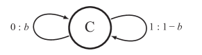
(a) Input Information Reservoir

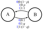
(b) Input-Output Transducer

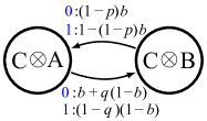
(c) Output Information Reservoir

Figure 1: (a) Hidden Markov model that generates a biased coin input string ${x}_{t}{x}_{t+1}\ldots$ with bias $\Pr({X}=0)=b$. Edge labels ${x}:p$ indicate a state-to-state transition of probability $p$ that emits symbol ${x}$. (b) The information ratchet’s transducer. Transducer edge labels ${x}|{x}^{\prime}:p$ indicate a state-to-state transition of probability $p$ taken on reading input symbol ${x}$ that emits symbol ${x}^{\prime}$. (c) The HMM that results from the transducer (b) operating on the input (a). The HMM describes the output string ${x}_{0}\ldots{x}_{t-1}$ generated by the ratchet driven by a coin with bias $b$. (Reprinted from Ref. [24] with permission.)

To be explicit, the total work supplied by the ratchet and an input bit from a coin of bias $b$ is [24]:

$$\langle W\rangle =\frac{k_{\text{B}}T}{2}[(pb-q+qb)\ln{\left(\frac{q}{p}\right)}$$

$$\quad\quad+(1-b)q\ln(1-q)+pb\ln(1-p)]~{}.$$ (3)

Here, $p$ and $q$ are parameters controlling the ratchet’s detailed-balance thermodynamics and, ultimately, its functioning. The explicit role of the parameters is given in Figures 1(a)-(c) which depict the (unifilar) hidden Markov models (HMMs) for the input process, ratchet transducer, and output process, respectively. In fact, these models are $\epsilon$-machines of the input and output processes and the $\epsilon$-transducer of the controller. Let’s quickly review how these process models are defined [36].

Definition 1.

A process $\mathcal{P}$’s $\epsilon$-machine $M(\mathcal{P})$ is the tuple $\big{\{}\bm{\mathcal{S}},\{T^{({x})}:{x}\in\mathcal{A}\},\bra{\eta_{0}}\big{\}}$, where $\bm{\mathcal{S}}$ is $\mathcal{P}$’s minimal set of predictively optimal states or causal states, $T^{({x})}$ are the state-to-state transition matrices, $\mathcal{A}$ is the alphabet of generated symbols, and $\bra{\eta_{0}}$ is the initial probability distribution over the causal states.

$\epsilon$-Transducers are defined similarly, except their causal states capture how the output process is conditioned on the input process [37].

$\epsilon$-Machines are unifilar: There is at most one transition labeled with a given symbol leaving a state. A seemingly innocent syntactical property, unifilarity is key to directly calculating $\mathcal{P}$’s entropy rate $h_{\mu}$ from its $\epsilon$-machine representation $M$, as the causal-state averaged transition uncertainty:

$$h_{\mu}(M)\!=\!-\!\!\sum_{\sigma\in\bm{\mathcal{S}}}\Pr(\sigma)\!\!\sum_{\begin{subarray}{c}\sigma^{\prime}\in\bm{\mathcal{S}}\\ {x}\in\mathcal{A}\end{subarray}}\Pr(\sigma^{\prime}\!,{x}|\sigma)\log_{2}\Pr(\sigma^{\prime}\!,{x}|\sigma),$$ (4)

where $\Pr(\sigma)$ is the asymptotic state probability calculated from the internal-state Markov chain transition matrix and $\Pr(\sigma^{\prime},{x}|\sigma)$ is the symbol-labeled transition probability $T^{({x})}_{\sigma^{\prime},\sigma}$. Due our representing the ratchet’s input and output processes with their $\epsilon$-machines, unifilarity allows us to exactly calculate their entropy rates, $h_{\mu}$ and $h_{\mu}^{\prime}$, respectively:

$$h_{\mu} =\operatorname{H}(b)$$

$$\equiv-b\log_{2}b-(1-b)\log_{2}(1-b)$$ (5)

$$h_{\mu}^{\prime} =\frac{\operatorname{H}(b(1-p))}{2}+\frac{\operatorname{H}((1-b)(1-q))}{2}~{},$$ (6)

where $\operatorname{H}(b)$ is the (base $2$) binary entropy function [38].

Equations (3), (5), and (6) explicitly give the work done $\langle W\rangle$ and information change $h_{\mu}^{\prime}-h_{\mu}$ from input to output as a function of input process bias ($b$) and ratchet thermal dynamics ($p$ and $q$). Thus, in light of Eq. (2) and Table 1, we can exactly determine the ratchet’s thermodynamic function over all of the ratchet’s parameter range; see Ref. [24, Figs. 7 and 8].

Or, so it would seem. Let’s explore what happens when there are statistical fluctuations. Imagine that the information ratchet is implemented in a physical substrate with a finite number of degrees of freedom, so that fluctuations are present.

III Fluctuations in Steady State

Let’s first consider the ratchet’s input information reservoir, by way of introducing our general view of statistical fluctuations. Once input fluctuations are understood, we apply the analysis to describe its effect on ratchet functionality.

Shannon-McMillan-Breiman theory tells us that with probability close to one sequences ${x}_{0:\ell}={x}_{0}\ldots{x}_{\ell-1}$ generated by a stochastic process of entropy rate $h_{\mu}$ consist of realizations whose probabilities scale with length $\ell$ as $\Pr({x}_{0:\ell})\simeq 2^{-h_{\mu}\ell}$ . Said most simply, almost all sequences are almost equally probable. These sequences are in the so-called typical set:

$$A_{\epsilon}^{\ell}=\{w\in\mathcal{A}^{\ell}:2^{-\ell(h_{\mu}+\epsilon)}\leq\Pr(w)\leq 2^{-\ell(h_{\mu}-\epsilon)}\}~{},$$ (7)

where $\mathcal{A}^{\ell}$ is the set of length-$\ell$ words. It can be shown that, for a given $\epsilon\ll 1$ and sufficiently large $\ell$:

$$\Pr(w\in A_{\epsilon}^{\ell})\geq 1-\epsilon~{}.$$ (8)

In other words, the probability of seeing sequences in this set is close to one. This gives a precise and operational definition to what one means by “typical” behavior. In addition, as a consequence of Eqs. (7) and (8), the typical set has approximately $2^{\ell h_{\mu}}$ sequences: $\left|A_{\epsilon}^{\ell}\right|\simeq 2^{h_{\mu}\ell}$. This suggests two meanings for $h_{\mu}$: the decay rate of probability for words $w\in A_{\epsilon}^{\ell}$ and the growth rate of their number.

That said, stochastic processes do generate sequences outside their typical set. A 60%-40% biased coin for a large but finite number of flips typically produces sequences with near 60% Heads and 40% Tails. More precisely, for $\ell=1000$ flips and $\epsilon=0.01$ the typical set includes sequences having between $58.2\%$ and $61.7\%$ Heads in them. (See App. C for the details of such estimates.) By increasing the number of flips the percentage of observed Heads converges to $60\%$.

At the same time, though, the process can and does generate sequences with 55% Heads and 45% Tails. The occurrence of such atypical sequences are statistical fluctuations—any statistic calculated from them, such as a mean, will fluctuate from trial to trial or even, when locally averaged, within a single long realization. Importantly, the likelihood of these fluctuations is enhanced when examining relatively short-length realizations. (We return to this in drawing out the ultimate consequences.)

A key question, in light of these observations, is what is the range of fluctuations for a given process? Moreover, how are fluctuations affected by the input process’ structure and memory? By way of answering these questions and going beyond Shannon’s elementary theory for memoryless processes [40] and McMillan and Breiman’s focus on typical behaviors of memoryful process [41, 42], Refs. [43, 44] show how to calculate the entire spectrum of statistical fluctuations for structured processes via their $\epsilon$-machines. We recall only the minimal necessary methods from there, but note that they are familiar and widely used, being central to statistical mechanics, large deviation theory in mathematical statistics [45, 46], and the thermodynamic formalism in dynamical systems theory [47, 48].

To probe fluctuations in the informational and statistical properties of the input process $\mathcal{P}$, we could simply sample its behavior. However, we are particularly interested in behaviors outside the typical set. And, by Cramer’s theorem [49], the sequence subsets of interest are exponentially rare. That is, while we could use $M(\mathcal{P})$ to generate long realizations and simply wait to see all of $\mathcal{P}$’s statistical fluctuations, this takes an exponentially long time or an exponentially large number of trials. To circumvent this, we modify the process’ $\epsilon$-machine presentation $M(\mathcal{P})$. Let’s say that we are interested in a particular set of words outside of the typical set; let’s call this the $\beta$-set. Instead of using $M(\mathcal{P})$, as an alternative strategy we transform $M$ to a new $\epsilon$-machine $M_{\beta}$ that generates a new process whose set of typical sequences is the specific fluctuation subset of interest—the $\beta$-set—in the original process.

Thus, we consider the parameter $\beta$ as indexing $\mathcal{P}$’s fluctuation subsets ($\beta$-sets)—sequences that all share the same asymptotic decay rate in their probabilities; recall Eq. (7). At fixed $\beta$, $M_{\beta}$ itself generates a new process $\mathcal{P}_{\beta}$. As a side benefit, since $M_{\beta}$ is an $\epsilon$-machine we can appeal to a number of tools to efficiently calculate various informational properties directly [50]. The final step is to simply note that $M_{\beta}$’s information properties are those of the fluctuation $\beta$-set in the original process $\mathcal{P}$. Let’s now describe this procedure in the operational detail needed to explore fluctuations in thermodynamic function.

To study the fluctuation subsets—the $\beta$-sets—we consider the set $\mathcal{A}^{\ell}$ of all sequences of length $\ell$. The typical set is the subset of words $w\in\mathcal{A}^{\ell}$ for which $\frac{-\log_{2}\Pr(w)}{\ell}\approx h_{\mu}$. This suggests partitioning the set $\mathcal{A}^{\ell}$ itself into small fluctuation $\beta$-sets that we can then study individually. To implement this, to each sequence $w\in\mathcal{A}^{\ell}$ one associates an energy density:

$$U^{\ell}_{w}=\frac{-\log_{2}\Pr(w)}{\ell}~{},$$ (9)

mirroring the common Boltzmann weight in statistical physics: $\Pr(w)\propto e^{-U^{\ell}_{w}\ell}$ . In our setting of structured processes, there can be forbidden sequences $w$ for which $\Pr(w)=0$—those with infinite energy.

Naturally, different sequences $w$ and $v$ may lead to the same energy density, $U^{\ell}_{w}=U^{\ell}_{v}$. Realizing this, we use definition Eq. (9) to partition $\mathcal{A}^{\ell}$ into fluctuation subsets consisting of sequences with the same energy $U$. Energy in this statistical setting is merely a proxy for parametrizing classes of equal-probability-scaling sequences. In the limit of $\ell\to\infty$ we effectively partition $\mathcal{A}^{\infty}$ into a continuous family of subsets, each with a label $U$. The sequences in each subset all share the same decay rate. Recall that we defined a $\beta-$set in a similar manner: All the words in one of those partitions have the same decay rate, too. In fact, $U$ and $\beta$ are simply different ways to index the same family of partitions.

In the set of allowed energies $U^{\ell}=\left\{U^{\ell}_{w}:w\in\mathcal{A}^{\ell}\right\}$ energy values may appear repeatedly. Denote the count $|\{U_{w}^{\ell}=U:U_{w}^{\ell}\in U^{\ell}\}|$ of length-$\ell$ sequences $w$ with equal energy $U$ by $N(U_{w}^{\ell}=U)$. The associated sequence set is the process’ thermodynamic macrostate at energy $U$ and we define its entropy density:

$$S(U)=\lim_{\ell\to\infty}\frac{\log_{2}N(U_{w}^{\ell}=U)}{\ell}~{}$$ (10)

to monitor the range and likelihood of allowed sequences (or accessible energies). This definition closely mirrors that in statistical physics, where a macrostate’s thermodynamic entropy is proportional to the logarithm of the number of accessible microstates.

Appendix A shows that $S(U)$ is a well behaved concave function of $U$. From Eqs. (7) and (9), we see that the typical set is that subset in $\mathcal{A}^{\infty}$’s $U$-parametrized partition with entropy density $S(U)=h_{\mu}$. Let’s pursue this a bit further. Recall the two interpretations for entropy rate $h_{\mu}$. The first was as the decay rate of typical-set sequence probabilities. And, for an arbitrary fluctuation subset the decay rate was interpreted as the energy density $U$. The second interpretation was that $h_{\mu}$ was the growth rate of the number of sequences in the typical set. And, for an arbitrary fluctuation subset the growth rate was the entropy density $S(U)$. This comparison gives an alternative definition of the typical set: the only sequence subset for which the decay rate and growth rate are equal. For all the other fluctuation sets $S(U)<U$ and so they are rare, exponentially so.

To calculate a process’ spectrum of fluctuations—how $S$ (Eq. (10)) depends on $U$ (Eq. (9)) for the sequences outside $\mathcal{P}$’s typical set—we transform its $\epsilon$-machine $M$ to a new “twisted” $\epsilon$-machine $M_{\beta}$ whose typical set is $\mathcal{P}$’s fluctuation subset at $\beta$ [43, 44]. (Appendix A reviews the detailed construction of $M_{\beta}$.) Moreover, there is a one-to-one mapping between $\beta$ and $U$. This means that there is a well defined, invertible function $U(\beta)$. And so, varying $\beta$ between negative infinity and positive infinity sweeps over all the fluctuation subsets.

Operationally, using $M_{\beta}$ gives a direct way to calculate the thermodynamic entropy density and energy density as a function of $\beta$:

$$S(U(\beta))={h_{\mu}}(M_{\beta})~{},$$ (11)

$$U(\beta)=\frac{1}{\beta}({h_{\mu}}(M_{\beta})-\log{\widehat{\lambda}_{\beta}})~{},$$ (12)

where ${\widehat{\lambda}_{\beta}}$ is $M_{\beta}$’s transition matrix’s maximal eigenvalue. And, using the $\epsilon$-machine entropy rate expression in Eq. (4) gives a similarly direct way to calculate the thermodynamic entropy density. All in all, using $\mathcal{P}$’s $\epsilon$-machine leads to explicit expressions for the fluctuation spectrum of the process it generates: the range of fluctuations (energies $U(\beta$)) and the “sizes” $S(U)$ of its fluctuation subsets.

While this exposition on fluctuations may seem indirect, there is a rather simple and geometric description of the basic shape and properties of the fluctuation spectrum $S(U)$. First, at a given energy, $\beta$ is the slope of $S(U)$: $\beta=\partial S(U)/\partial U$. (Appendix A gives the proof.) Second, a process’ typical set occurs at the $U$ such that $\beta=1$. Third, a process’ most likely sequences occur at the extreme of $\beta\to\infty$. Since probability is associated with energy, we think of these sequences as a process’ ground states. That is, the lowest energy sequences are the most probable. Fourth, for an ergodic, finite-memory process $S(U)$ is a well behaved, convex function of $U$. Fifth, and finally, the latter implies that there is also a set of least probable or “high energy” sequences, found at $\beta\to-\infty$. And so, $\beta$ can be negative, indicating the statistical analog of the physics of population inversion. We now turn to illustrate these properties and their consequences for thermodynamic functioning.

IV Functional Fluctuations

We are ready to bring together our identification of thermodynamic functionality in Sec. II, which ultimately derived from Eq. (2)’s Second Law for information processing, with Eqs. (11)’s and (12)’s analysis of statistical fluctuations in Sec. III. With the connection made, we then go on to calculate the likelihood of functional fluctuations.

IV.1 Setting

Recall the ratchet introduced in Sec. II, but with its Markov dynamic parameters $p=0.2$ and $q=0.6$ and with an input reservoir generating independent and identically distributed (IID) symbol sequences of bias $b=0.9$. If we operate the input reservoir for a sufficiently long time, with high probability we observe a sequence that has nearly $90\%$ $0$s in it. Using Eqs. (3), (5), and (6) we see positive work $\langle W\rangle>0$ and positive entropy production $h_{\mu}^{\prime}-h_{\mu}>0$, describing the ratchet’s transforming the input process’ typical sequences to the output process. Then, by Table 1, the ratchet typically operates as an engine. The work $\langle W\rangle$, too, is function of input-process typical set and the ratchet parameters.

As we emphasized earlier, it is not always the case that the input reservoir generates ideal typical sequences. It also generates sequences outside the typical set. For example, given the parameters quoted, it can generate long sequences with $70\%$ $0$s. Let’s consider the case where a long atypical sequence $w$ is generated for which $\frac{-\log_{2}\Pr(w)}{\ell}=U$, but $U\neq h_{\mu}$. What is the functionality of ratchet in this case?

The key here is to find an alternate process that typically generates sequences with energy density $U$ and then analyze the ratchet’s response to them. As noted above, for every fluctuation subset with energy density $U$ there is a unique $\beta$ such that the new process’ $M_{\beta}$ generates this fluctuation subset typically. Using Eqs. (10) and (11), the entropy rate $h_{\mu}$ of the new process is $S(U)$. With this method we can directly calculate $h_{\mu}$, $h_{\mu}^{\prime}$, and $\langle W\rangle$ for $M_{\beta}$ and, consequently, for the particular fluctuation subset at $U$. Putting these quantities together, we then identify the ratchet’s functionality via Table 1.

To keep distinct properties distinct and so reduce confusion, we must emphasize a point about notation and interpretation. The previous section introduced a parameter $\beta$ for a given process. Despite its mathematical similarity to the inverse temperature in statistical mechanics and historical reasons for using that notation, for ease of understanding $\beta$ should be thought of simply as a index of various fluctuation subsets generated by the given process. (Technically, we can do this since $U$ indexes the fluctuation subsets and $U(\beta)$ is monotonic in $\beta$.) Equally important, the input process parameter $\beta$ and the output $\beta^{\prime}$ parameter are conceptually distinct from the temperature $T$ of the ratchet’s thermal reservoir; e.g., as used in Eqs. (2) and (3). In short, at this point in our analysis, none of these three variables should be conflated notationally nor physically.

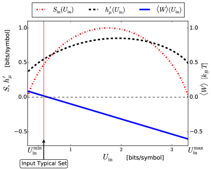
Figure 2: Fluctuation spectra under a thermodynamic transformation implemented by Ref. [24]’s information ratchet with parameters $p=0.2$ and $q=0.6$ driven by an IID input source with bias $b=0.9$: Input process Shannon entropy rate $h_{\mu}=S_{\text{in}}$ versus fluctuation-subset label (energy) $U_{\text{in}}$ (alternating dashed line), resulting output process’ $h_{\mu}^{\prime}$ versus $U_{\text{in}}$ (dashed line), and the average work $\langle W\rangle$ versus $U_{\text{in}}$ (solid line).

IV.2 Input, Ratchet, and Work Ratchet Fluctuations

The first step is to determine the fluctuation spectrum for the input process and then the spectrum of the ratchet’s response. Recall that we are considering the behavior of Ref. [24]’s information ratchet, but now as we sweep $\beta$ we control which subsets outside the typical set we focus on and consequently which fluctuation subset we analyze. For the analysis, recall that the input and output processes are specified by the unifilar HMMs in Figs. 1(a) and 1(c), respectively.

As $\beta$ sweeps from $-\infty$ to $\infty$, by using the new $\epsilon$-machine $M_{\beta}$ we can analyze all of the fluctuation subsets generated by the input process. A result of the method in App. A, $M_{\beta}$ is the same as the $\epsilon$-machine in Fig. 1(a), except that we change $b$ to $\widehat{b}=b^{\beta}/\left(b^{\beta}+(1-b)^{\beta}\right)$. The input process’ thermodynamic entropy density $S_{\mathrm{in}}(U_{\mathrm{in}})$ and energy density $U_{\mathrm{in}}$ are calculated from Eqs. (11) and (12). Then, feeding the new process to the ratchet, $\langle W\rangle$ can be calculated from Eq. (3), again by changing $b$ to $\widehat{b}$. We denote this work quantity $\langle W\rangle(U_{\mathrm{in}})$. By feeding the new input process to the ratchet the output process’ $\epsilon$-machine is the same as the $\epsilon$-machine in Fig. 1(c) but we again change $b$ to $\widehat{b}$. The entropy rate of this output process is denoted by $h_{\mu}^{\prime}(U_{\mathrm{in}})$. To predict the thermodynamic effect of feeding in the fluctuation subset with energy density $U_{\mathrm{in}}$ instead of feeding it with a typical sequence, we substitute $S_{\mathrm{in}}(U_{\mathrm{in}})$, $h_{\mu}^{\prime}(U_{\mathrm{in}})$, and $\langle W\rangle(U_{\mathrm{in}})$ for $h_{\mu}$, $h_{\mu}^{\prime}$, and $\langle W\rangle$, respectively, in the informational Second Law Eq. (2).

Figure 2 puts these altogether, showing the input process’ fluctuation spectrum $S_{\mathrm{in}}(U_{\mathrm{in}})$, the output process’ spectrum $h_{\mu}^{\prime}(U_{\mathrm{in}})$, and the dissipated work $\langle W\rangle$ versus fluctuation energy density $U_{\mathrm{in}}$. There are several observations to make first, before we associate thermodynamic function.

First, let’s locate the input typical set. It occurs at a $U$ such that the slope $\beta=1$ on $S_{\text{in}}(U_{\mathrm{in}})$. The figure identifies it with vertical line, so labeled.

Second, the input process’ ground states occur as $\beta\to\infty$. As a consequence of Eq. (9) the ground state at $U_{\text{in}}^{\text{min}}$ corresponds to the sequence with the highest probability. In this case this is the all-$0$s sequence and consequently $U_{\text{in}}^{\text{min}}=-\log_{2}(b)\simeq 0.152$. The other extreme is at $U_{\text{in}}^{\text{max}}$, corresponding to the lowest probability, allowed sequence. In this case it is the all-$1$s sequence. Consequently, $U_{\text{in}}^{\text{max}}=-\log_{2}(1-b)\simeq 3.32$. Visualized as slopes on $S_{\text{in}}$ respectively, these extremes occur at the very left and very right portion of the curves, respectively. Note that there is only a single sequence associated with $U_{\text{in}}^{\text{max}}$ and only one with $U_{\text{in}}^{\text{min}}$. By using Eq. (10) we have $S_{\text{in}}(U_{\text{in}}^{\text{max}})=S_{\text{in}}(U_{\text{in}}^{\text{min}})=0$, as seen in the figure.

Third, note that the input fluctuation spectrum $S_{\text{in}}(U_{\text{in}})$ is rather familiar. The parametrized representation of the function $S_{\text{in}}(U_{\text{in}})$ in terms of $\beta$ is the well known fluctuation spectrum of a biased coin. (See App. E.)

Fourth, the spectrum of output entropy rates $h_{\mu}^{\prime}(U_{\text{in}})$ ranges from $U_{\text{in}}^{\text{min}}$ to $U_{\text{in}}^{\text{max}}$, but does not vanish at these extremes. This indicates stochasticity in the output process that is added by the ratchet itself to the zero entropy-rate input sequences there. More on the functional consequences, shortly.

Fifth and finally, to complete the task, we must determine the average work $\langle W\rangle$ as a function of energy $U_{\text{in}}$. From the figure, we see that the dissipated work $\langle W\rangle$ is linear in the energy density $U_{\text{in}}$. (Appendix E derives this.)

IV.3 A Spectrum of Thermodynamic Function

So much for statistical fluctuations in the operation of the system’s components individually. What does the informational Second Law tell us about the range of thermodynamic functioning—Engine, Eraser, or Dud—the ratchet performs when exhibiting these fluctuations? With the detailed analysis of the input and output process fluctuation spectra and their associated energies, we are ready to invoke the informational Second Law to determine the ratchet’s effective thermodynamic function for various fluctuations.

Figure 3 summarizes this functional identification, using the trade-offs between input-output process entropy change and dissipated work $\langle W\rangle$ specified by Eq. (2) and the thermodynamic functioning identified in Table 1 to label the various functional regimes parametrized by $U_{\text{in}}$. These fall into four regimes, from left to right, increasing $U_{\text{in}}$, the ratchet operates as an engine (green), a dud (yellow), an eraser (red), and then again as a dud (yellow).

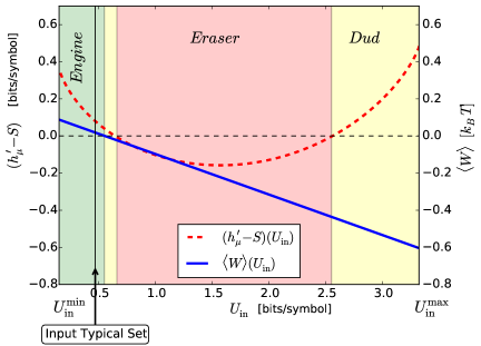
Figure 3: Fluctuations in thermodynamic functioning: Using the new Second Law of information processing and Table 1 to identify how different fluctuation subsets operate within the information ratchet as a function of subset label $\beta\propto e^{-U}$. Engine: $h_{\mu}^{\prime}(U_{\text{in}})-S_{\text{in}}(U_{\text{in}})>0$ and $\langle W\rangle>0$; Eraser: $h_{\mu}^{\prime}(U_{\text{in}})-S_{\text{in}}(U_{\text{in}})<0$ and $\langle W\rangle<0$; and Dud: otherwise. Note that the range of the horizontal axis extends only over the range of $U_{\text{in}}$, since that is all that can be accessed by input fluctuations; cf. Fig. 2.

To better understand how the ratchet operates thermodynamically, consider the ground state of the input process; which as just noted has only a single member, the all-$0$ sequence with zero entropy rate $S(U_{\text{in}}^{\text{min}})=0$. If we feed this sequence into the ratchet, the ratchet adds stochasticity which appears in the output sequence. The first $0$ fed to the ratchet leads to a $0$ on the output. For the next $0$ fed-in, with probability $p$ the ratchet outputs $1$ and with probability $1-p$ it outputs $0$. The entropy rate of output sequence then is $h_{\mu}^{\prime}(U_{\text{in}}^{\text{min}})=\frac{1}{2}H(p)\simeq 0.36$. (See also the left end of $h_{\mu}^{\prime}$ in Fig. 2.)

To generate this sequence we simply use the $\epsilon$-machine in Fig. 1 with $b=1$. With this biased process as input, using Eq. (3) we find $\langle W\rangle(U_{\text{in}}^{\text{min}})\simeq 0.0875>0$. Table  1 then tells us that if we feed the ground state of the input process to the ratchet, it functions as an engine. At the other extreme $U_{\text{in}}^{\text{max}}$, the only fluctuation subset member is the all-$1$s sequence with $S(U_{\text{in}}^{\text{max}})=0$. Again, the ratchet adds stochasticity and the output has $h_{\mu}^{\prime}(U_{\text{in}}^{\text{max}})=\frac{1}{2}H(q)\simeq 0.485$. (See also the right end of $h_{\mu}^{\prime}$ in Fig. 2.) To generate this input sequence we simply use the $\epsilon$-machine in Fig. 1 with $b=0$. With this process as an input, we use Eq. (3) again and find negative work $\langle W\rangle(U_{\text{in}}^{\text{max}})\simeq-0.6$. Table  1 now tells us that feeding in this extreme sequence (input fluctuation) the ratchet functions as a dud.

We conclude that the ratchet’s thermodynamic functioning depends substantially on fluctuations and so will itself fluctuate over time. The Engine functionality occurs only at relatively low input fluctuation energies, seen on Fig. 2’s left side, and encompasses the typical set, as a consequence of our design. Rather nearby the Engine regime, though, is a narrow one of no functioning at all—a Dud. In fact, though the ratchet was designed as an Engine, we see that over most of the fluctuations, with the given parameter setting the ratchet operates as an Eraser.

Finally, App. D shows that the maximum work, over all fluctuation subsets—all $\beta$ or all allowed $U$s—is independent of the input process bias. This is perhaps puzzling as bias clearly controls the ratchet’s thermodynamic behavior. Thus, assuming an IID input, the maximum work is a property of the ratchet itself and not the input, playing a role rather analogous to how Shannon’s channel capacity is a channel property.

IV.4 Probable Functional Fluctuations

How probable are fluctuations in thermodynamic function? The answer, at first sight, is not entirely obvious, given that we are asking a question about deviations from the typical set and so are asking about the likelihood of a property of rare realizations. Indeed, statistical variations in this or that property might not be practically observable at all. We now show that the functional fluctuations are, in fact, quite observable even at relatively long word lengths, such as $\ell=100$.

To answer this we first need to address how likely we are to observe a fluctuation. The large-deviation rate function $I(U)$ provides the answer as it gives the probability of the subset of sequences with the same energy $U$. The Gartner-Ellis theorem [52, 45, 46] says that the probability of a sequence occurring in a fluctuation set with energy density $U$ is determined by:

$$I(U)=\lim_{\ell\to\infty}-\frac{\log_{2}\Pr(U^{\ell})}{\ell}~{}.$$

That is, the subset probability scales exponentially: $\Pr(U^{\ell}=U)=\exp(-I(U)\ell)+\mathscr{O}(\ell)$, where $\mathscr{O}(\cdot)$ decays faster than any exponential.

Importantly, we can directly determine the large-deviation rate function $I(U)$ as it is directly related to the fluctuation spectrum $S(U)$ just derived in Eqs. (12) and (11) [44]:

$$I(U)=U-S(U)~{}.$$ (13)

To understand this a bit more, let’s compare to $S(U(\beta))$. For large $\ell$, as noted above, $\beta=1$ indicates the typical set, its sequences’ probabilities decay at the entropy rate $h_{\mu}$ and the probability of observing a realization in the typical set converges to $1$. Thus, $I(U)=0$ there and $S(U)=U$. For other fluctuation sets with energy density $U$, we expect the probability of the fluctuation subset at $U$ to vanish with increasing length $\ell$ and $I(U)$ indicates exactly how fast this decay is.

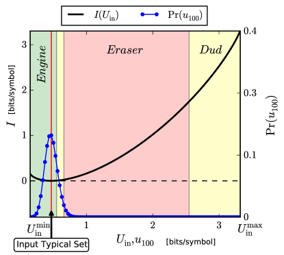
Figure 4: Decay rate of probability of fluctuations in thermodynamic functioning: Large-deviation rate function $I(U_{\text{in}})$ (solid black line) and the probability $\Pr(u_{100})$ of fluctuation subsets for length $\ell=100$ input realizations (dotted blue line).

So, now we can ask how likely the ratchet is to fluctuate between its possible thermodynamic modalities. This is determined from the large deviation rate function $I(U)$ of Eq. (13), which Fig. 4 plots as a function of $U_{\text{in}}$. As the figure shows, when realizations from the typical set are fed in, the ratchet functions as an Engine. Also, this subset happens with zero large deviation rate. At the limit of infinite length the probability of the typical set goes to one and the probability of fluctuation subsets vanishes. The ratchet operates as an engine over long times with probability one. In reality, though, we only work with finite length sequences. And so, the operant question here is, are these functional fluctuations observable at finite lengths? As we alluded to much earlier, short sequences enhance their observation.

Consider the input process in Fig. 1(a) and assume the input’s realization length is $\ell=100$. For this case we have $2^{100}$ distinct input sequences that are partitioned into $101$ fluctuation subsets with different energy densities—subsets of sequences with $n$ $0$s and $100-n$ $1$s for $n=0,1,\ldots,100$. Let’s calculate the probability of each of these fluctuations subsets occurring. The probability of each versus its energy is shown in Fig. 4 as the blue dotted line. To distinguish it from the energy density of fluctuation subsets at infinite length we label the energy density of each of these sets with $u_{100}$, the index $100$ reminds us that we are examining input sequences of length $\ell=100$. There are $101$ blue points on the figure, each representing one of the fluctuation subsets. From $101$ fluctuation subsets, if we fed $13$ of them (the first 13 blue points in the left of the figure) to the ratchet, the ratchet functions as an Engine. This means for the other $87$ fluctuation subsets the ratchet functions as a Dud or Eraser. By calculating the probabilities we see by feeding an input sequence with length $100$, with approximately $80\%$ probability the ratchet functions as an Engine, with approximately $17.8\%$ probability it functions as a Dud, and with $2.2\%$ probability functions as an Eraser.

V Conclusion

We synthesized statistical fluctuations—as entailed in Shannon’s Asymptotic Equipartition Property [38] and large deviation theory [52, 45, 46]—and functional thermodynamics—as determined using the new informational Second Law [24]—to predict spontaneous variations in thermodynamic functioning. In short, there is simultaneous, inherently parallel, thermodynamic processing that is functionally distinct and possibly in competition. This strongly suggests that, even when in a nonequilibrium steady state, a single nanoscale device or biomolecule can be both an engine and an eraser. And, we showed that these functional fluctuations need not be rare. The conclusion is that functional fluctuations should be readily observable and the prediction experimentally testable.

A main point motivating this effort was to call into question the widespread habit of ascribing a single functionality to a given system and, once that veil has lifted, to appreciate the broad consequences. To drive them home, since biomolecular systems are rather like the information ratchet here, they should exhibit, measurably different thermodynamic functions as they behave. If this prediction holds, then the biological world is vastly richer than we thought and it will demand of us a greatly refined vocabulary and greatly improved theoretical and experimental tools to adequately probe and analyze this new modality of parallel functioning.

That said, thoroughness forces us to return to our earlier caveat (Sec. IV) concerning not conflating various “temperatures”. If we give the input information reservoir and the output information reservoir physical implementations, then the fluctuation indices $U_{\text{in}}$ and $U_{\text{out}}$ take on thermal physical meaning and so can be related to the ratchet’s thermodynamic temperature $T$. Doing so, however, would take us too far afield here, but it will be necessary for a complete understanding.

Equally important, the theoretical scaffolding used above in the service of illustrating parallel thermodynamic functioning invokes a number of simplifications. Perhaps the main one is the use of time-asymptotic quantities, such as the Shannon entropy rate and large deviation rate function. A proper analysis requires carefully working in the finite-time, finite-length sequence regime—the very regime that enhances statistical fluctuations. This task is markedly more challenging and will be attempted elsewhere. However, the central goal has been to explicate the main ideas and these are robust to the simplifications employed. Moreover, we drove the ratchet with atypical input sequences, assuming that the ratchet responded typically. However, in addition, we could have explored the ratchet’s atypical behavior in response to input typical sequences. Or both: analyze the atypical transduction of atypical inputs.

Similarly looking forward, there are sister challenges. First, note that technically speaking we introduced a fluctuation theory for memoryful stochastic transducers, but by way of the example of Ref. [24]’s information ratchet. A thoroughgoing development must be carried out in much more generality using the tools of Refs. [37], [44], and [53], if we are to fully understand the functionality of thermodynamic processes that transform inputs to outputs, environmental stimulus to environmental action.

Second, the role of Jarzynski-Crooks theory for fluctuations in thermodynamic observables needs to be made explicit and directly related to statistical fluctuations, in the sense emphasized here. One reason is that their theory bears directly on controlling thermodynamic systems and the resulting macroscopic fluctuations. To draw the parallel more closely, we could drive the ratchet parameters $p$ and $q$ and input bias $b$ between different functional regimes and monitor the entropy production fluctuations to test how the theory fares for memoryful processes. In any case, efficacy in control will also be modulated by statistical fluctuations.

Not surprisingly, there is much to do. Let’s turn to a larger motivation and perhaps larger consequences to motivate future efforts.

As just noted, fluctuations are key to nanoscale physics and molecular biology. We showed that fluctuations are deeply implicated both in identifying thermodynamic function and in the very operation of small-scale systems. In fact, fluctuations are critical to life—its proper and robust functioning. The perspective arising from parallel thermodynamic function is that, rather than fluctuations standing in contradiction to life processes, potentially corrupting them, there may be a positive role for fluctuations and parallel thermodynamic functioning. Once that is acknowledged it is a short step to realize that biological evolution [54] may have already harnessed them to good thermodynamic effect. Manifestations are clearly worth looking for.

It now seems highly likely that fluctuations engender more than mere health and homeostasis. It is a commonplace that biological evolution is nothing, if not opportunistic. If so, then it would evolve cellular biological thermodynamic processes that actively leverage fluctuations. Mirroring Maxwell’s Demon’s need for fluctuations to operate, biological evolution itself advances only when there are fluctuations. For example, biomolecular mutation processes engender a distribution of phenotypes and fitnesses; fodder for driving selection and so evolutionary innovation. This, then, is Darwin’s Demon—a mechanism that ratchets in favorable fluctuations for positive thermodynamic and then positive survival benefit. The generality of results and methods here give new insight into thermodynamic functioning in the presence of fluctuations that should apply at many different scales of life, including its emergence and evolution.

Appendix A Process Fluctuations from the Twisted $\epsilon$-Machine

A process’ fluctuation spectrum is calculated from its twisted $\epsilon$-machine. Introducing the latter requires briefly recalling several important and relevant concepts. Though the following closely tracks Refs. [43, 44], the synopsis here is relatively self contained as far as basic calculations are concerned.

The Shannon block entropy is a linear average of the sequence self-informations $-\log_{2}\Pr(w)$. The closely related Renyi block entropy is the most general entropy that is both additive over independent distributions (extensive) and a geometric average [55]:

$$\operatorname{H}_{\beta}(\ell) =\operatorname{H}_{\beta}[X_{0:\ell}]$$

$$=\frac{1}{1-\beta}\log_{2}\sum_{\{w\in\mathcal{A}^{\ell}\}}(\Pr(w))^{\beta}~{},$$ (14)

where $\beta$ is an arbitrary real number that allows us to “focus” on sequence subsets parametrized by probability—or, equivalently, by energy $U_{w}=-\log\Pr(w)$. We see that $\beta$ is analogous to inverse temperature and we can interpret the sum $\sum_{\{w\in\mathcal{A}^{\ell}\}}(\Pr(w))^{\beta}$ as the partition function:

$$\mathcal{Z}_{\ell}(\beta)=\sum_{\{w\in\mathcal{A}^{\ell}\}}e^{-\beta(-\ln\Pr(w))}~{}.$$ (15)

Now, we are ready to define a process’ twisted $\epsilon$-machine, which is determined from the process’ $\epsilon$-machine. It is the analog of the escort or twisted distributions of large deviation theory [52, 45, 46], but adapted to our setting of structured processes.

Definition 2.

A process $\mathcal{P}$’s twisted $\epsilon$-machine is the parametrized family of $\epsilon$-machines $M_{\beta}=\big{\{}\bm{\mathcal{S}},\{\textbf{S}_{\beta}^{({x})}:{x}\in\mathcal{A}\},\bra{\widehat{\eta}_{0}}\big{\}}$, where the components are the same as $\mathcal{P}$’s $\epsilon$-machine $M(\mathcal{P})$, except that there is an inverse temperature parameter $\beta$ and a new, parametrized transition dynamic:

$$\big{(}\textbf{S}^{({x})}_{\beta}\big{)}_{ij}=\frac{\big{(}\textbf{T}^{({x})}_{\beta}\big{)}_{ij}({\widehat{\mathbf{r}}_{\beta}})_{j}}{{\widehat{\lambda}_{\beta}}({\widehat{\mathbf{r}}_{\beta}})_{i}}~{}.$$ (16)

$\mathcal{P}$’s $\epsilon$-machine transition matrices $T_{ij}^{(x)}=\Pr(\sigma_{j},x|\sigma_{i})$ are transformed to:

$$\big{(}\textbf{T}^{({x})}_{\beta}\big{)}_{ij} =e^{\beta\ln{\Pr(\sigma_{j},{x}|\sigma_{i})}}$$

$$=\big{(}\Pr(\sigma_{j},{x}|\sigma_{i})\big{)}^{\beta}~{}.$$

We calculate its eigenvectors and eigenvalue as follows. Form $M_{\beta}$’s internal causal-state transition matrix:

$$\textbf{T}_{\beta}=\sum_{{x}\in\mathcal{A}}T^{({x})}_{\beta}~{}.$$

Then ${\widehat{\mathbf{l}}_{\beta}}$ (${\widehat{\mathbf{r}}_{\beta}}$) is the left (right) eigenvector of $\textbf{T}_{\beta}$, associated with ${\widehat{\lambda}_{\beta}}$:

$${\widehat{\mathbf{l}}_{\beta}}\textbf{T}_{\beta} ={\widehat{\lambda}_{\beta}}{\widehat{\mathbf{l}}_{\beta}}$$

$$\textbf{T}_{\beta}{\widehat{\mathbf{r}}_{\beta}} ={\widehat{\lambda}_{\beta}}{\widehat{\mathbf{r}}_{\beta}}~{},$$

where ${\widehat{\lambda}_{\beta}}$ is $\textbf{T}_{\beta}$’s maximum eigenvalue. We chose the eigenvectors such that:

$${\widehat{\mathbf{l}}_{\beta}}\cdot{\widehat{\mathbf{r}}_{\beta}}=1~{}.$$ (17)

The new initial state probability distribution $\bra{\widehat{\eta}_{0}}$ is the normalized left eigenvector of $\sum_{\{{x}\}}{\textbf{S}}^{({x})}_{\beta}$.

Let $\Pr(w)$ denote the probability that the original $\epsilon$-machine $M$ generates the length-$\ell$ sequence $w$. Then the probability of the same sequence being generated by $M_{\beta}$ is [43, 44]:

$$\mathcal{Q}_{\beta}(w)=\frac{(\Pr(w))^{\beta}}{\mathcal{Z}(\beta)}~{}.$$ (18)

It can be shown [43, 44] that generating the twisted distribution $\mathcal{Q}_{\beta}(\cdot)$ is equivalent to generating a new process whose typical set is the fluctuation subset at $U=U(\beta)$ in the original process, where:

$$U(\beta)=\frac{1}{\beta}({h_{\mu}}(M_{\beta})-\log{\widehat{\lambda}_{\beta}})~{}.$$ (19)

This relates the energy and entropy densities, since the latter monitors the set’s growth rate; that is, $S(U)={h_{\mu}}(M_{\beta})$. Thus, by varying $\beta$ we choose which fluctuation subset $U(\beta)$ to focus in on. Critically, though, we have a new $\epsilon$-machine $M_{\beta}$ for which that subset is typical and so generated with high probability.

The fluctuation subset parameter $\beta$ is $S(U)$’s slope, illustrating that $S(U)$ is well behaved. Proof of convexity is found in the references cited above.

Theorem 1.

$\beta=\text{d}S/\text{d}U$.

Proof.

$$\frac{{\rm d}{\widehat{\lambda}_{\beta}}}{{\rm d}\beta} =\sum_{i,j}({\widehat{\mathbf{l}}_{\beta}})_{j}\frac{{\rm d}({\textbf{T}}_{\beta})_{ij}}{{\rm d}\beta}({\widehat{\mathbf{r}}_{\beta}})_{j}$$

$$=\frac{1}{\beta}\sum_{i,j}({\widehat{\mathbf{l}}_{\beta}})_{j}({\textbf{T}}_{\beta})_{ij}({\widehat{\mathbf{r}}_{\beta}})_{j}\log({\textbf{T}}_{\beta})_{ij}.$$ (20)

From Eqs. (16) and (17) one sees that:

$$({\widehat{\mathbf{l}}_{\beta}})_{j}({\textbf{T}}_{\beta})_{ij}({\widehat{\mathbf{r}}_{\beta}})_{j}={\widehat{\lambda}_{\beta}}({\textbf{P}_{\beta}})_{i}({\textbf{S}_{\beta}})_{ij}~{},$$

which defines $\textbf{P}_{\beta}$. Using this in Eq. (Proof) gives:

$$\frac{1}{{\widehat{\lambda}_{\beta}}}\frac{{\rm d}{\widehat{\lambda}_{\beta}}}{{\rm d}\beta} =\frac{1}{\beta}\sum_{i,j}({\textbf{P}_{\beta}})_{i}({\textbf{S}_{\beta}})_{ij}\log({\textbf{T}}_{\beta})_{ij}$$

$$=\frac{1}{\beta}\sum_{i,j}({\textbf{P}_{\beta}})_{i}({\textbf{S}_{\beta}})_{ij}\left[\log({\textbf{S}_{\beta}})_{ij}+\log{\widehat{\lambda}_{\beta}}\right.$$

$$\quad\quad\left.+\log({\widehat{\mathbf{r}}_{\beta}})_{i}-({\widehat{\mathbf{r}}_{\beta}})_{j}\right]$$

$$=-\frac{S(U(\beta))}{\beta}+\frac{\log{{\widehat{\lambda}_{\beta}}}}{\beta}$$

$$\quad+\frac{1}{\beta}\sum_{i,j}({\textbf{P}_{\beta}})_{i}({\textbf{S}_{\beta}})_{ij}\left[\log({\widehat{\mathbf{r}}_{\beta}})_{i}-({\widehat{\mathbf{r}}_{\beta}})_{j}\right].$$ (21)

To obtain the first term above, the definition of entropy is used and for the second term one makes use of:

$$\sum_{i,j}({\textbf{P}_{\beta}})_{i}({\textbf{S}_{\beta}})_{ij} =\sum_{j}({\textbf{P}_{\beta}})_{j}$$

$$=\sum_{j}({\widehat{\mathbf{r}}_{\beta}})_{j}({\widehat{\mathbf{l}}_{\beta}})_{j}$$

$$={\textbf{l}_{\beta}}\cdot{\textbf{r}_{\beta}}$$

$$=1~{}.$$

Now, using:

$$\sum_{i}({\textbf{P}_{\beta}})_{i}({\textbf{S}_{\beta}})_{ij}=({\textbf{P}_{\beta}})_{j}=({\widehat{\mathbf{r}}_{\beta}})_{j}({\widehat{\mathbf{l}}_{\beta}})_{j}~{},$$

the third and the fourth terms in Eq. (Proof) simply cancel, and one arrives at:

$$\frac{{\rm d}}{{\rm d}\beta}\,(\log{\widehat{\lambda}_{\beta}})=-U(\beta)~{}.$$ (22)

Then one may take $S(\cdot)$ as a function of $\beta$. Multiplying both sides of Eq. (19) by $\beta$ and differentiating both sides with respect to $\beta$, one obtains:

$$U+\beta\frac{{\rm d}U}{{\rm d}\beta}=\frac{{\rm d}S}{{\rm d}\beta}-\frac{{\rm d}}{{\rm d}\beta}\,(\log{\widehat{\lambda}_{\beta}}),$$

Using Eq. (22), one finds:

$$\beta =\frac{{{\rm d}S}/{{\rm d}\beta}}{{{\rm d}U}/{{\rm d}\beta}}$$

$$=\frac{{\rm d}S}{{\rm d}U}~{}.$$ (23)

Thus, $\beta$ indeed plays the same role here as the inverse temperature in statistical physics. One consequence of Eq. (Proof) is that $S(\cdot)$ is a well behaved function. From Def. 2 the typical set is found at $\beta=1$. And, this means that at the typical set we have $\mathrm{d}S/\mathrm{d}U=1$.

Appendix B Biased Coin Fluctuation Spectrum

First, recall Eq. (19):

$$S(U(\beta))=\beta U(\beta)+\log\lambda_{\beta}~{}.$$

Calculating the maximal eigenvalue $\widehat{\lambda}_{\beta}$, we find:

$$\log\lambda_{\beta}=\log_{2}(b^{\beta}+(1-b)^{\beta})~{}.$$

Second, for the entropy density recall that:

$$S(U(\beta))=h_{\mu}(M_{\beta})~{}.$$

Substituting $M_{\beta}$ bias $\widehat{b}=b^{\beta}/(b^{\beta}+(1-b)^{\beta}$ into Eq. (5), we find:

$$S(U(\beta))=- \left(\frac{b^{\beta}}{b^{\beta}+(1-b)^{\beta}}\log_{2}\frac{b^{\beta}}{b^{\beta}+(1-b)^{\beta}}\right.$$

$$\left.+\frac{(1-b)^{\beta}}{b^{\beta}+(1-b)^{\beta}}\log_{2}\frac{(1-b)^{\beta}}{b^{\beta}+(1-b)^{\beta}}\right)~{}.$$ (24)

It is straightforward, now, to calculate $U$ from these:

$$U(\beta) =\frac{-b^{\beta}}{b^{\beta}+(1-b)^{\beta}}\log_{2}(b)$$

$$\quad\quad+\frac{-(1-b)^{\beta}}{b^{\beta}+(1-b)^{\beta}}\log_{2}(1-b)~{}.$$ (25)

Plotting Eq. (24) against Eq. (25) gives the biased coin fluctuation spectrum shown in Fig. 2.

Appendix C Typical Set for a Biased Coin

What is $A_{\epsilon}^{(\ell)}$ for a biased coin with bias $b$? The typical set is defined by;

$$A_{\epsilon}^{(\ell)}=\{w\in\mathcal{A}^{\ell}:2^{-\ell(h_{\mu}+\epsilon)}\leq\Pr(w)\leq 2^{-\ell(h_{\mu}-\epsilon)}\}~{}.$$

The probability of a biased coin generating a particular sequence $w$ with $k$ heads is $b^{k}(1-b)^{(\ell-k)}$. And so, for $w$ to be in the typical set we must have:

$$\ell b-\frac{\ell\epsilon}{\log{\frac{b}{1-b}}}\leq k\leq\ell b+\frac{\ell\epsilon}{\log{\frac{b}{1-b}}}~{}.$$

Since $k$ is an integer:

$$\left\lceil\ell b-\frac{\ell\epsilon}{\log{\frac{b}{1-b}}}\right\rceil\leq k\leq\left\lfloor\ell b+\frac{\ell\epsilon}{\log{\frac{b}{1-b}}}\right\rfloor~{}.$$

For example, in the case where $\ell=1000$, $b=0.6$, and $\epsilon=0.01$, we have:

$$582\leq k\leq 617~{}.$$

This means that those length $\ell=1000$ sequences with $582$ to $617$ Heads are in the typical set.

Appendix D Maximum Work is Independent of Input Process

The maximum work $\widehat{W}$ done by the information ratchet over all fluctuation subsets (parametrized by $\beta$, say) is independent of the given IID binary input process. Direct calculation gives:

$$\widehat{W} =\max_{\beta}\langle W\rangle$$

$$=\begin{cases}\widehat{W}^{-}\equiv k_{\text{B}}T\big{(}-q\log(p/q)-q\log(1-q)\big{)}&c<0\\ \widehat{W}^{+}\equiv k_{\text{B}}T\big{(}p\log(p/q)-p\log(1-p)\big{)}&c\geq 0\\ \end{cases}~{}.$$

where $c=(p+q)\log(q/p)+p\log(1-p)-q\log(1-q)$.

Appendix E Work is Linear in Energy Density

Recall the energy density $U$ parametrizes the fluctuation subsets. Here, we show that the work $\langle W\rangle$ is linear across the $U$-fluctuation classes:

$$\langle W\rangle(U)=\frac{k_{\text{B}}T}{2}\left(cU+U_{0}\right)~{},$$

where:

$$U_{0} =\tfrac{1}{2}\widehat{W}^{-}+c\times\frac{\log(1-b)}{\log(1-b)-\log b}~{}.$$

To see this, we first calculate the work $W(\beta)$ from Eq. (3):

$$W(\beta)=\frac{k_{\text{B}}T}{2}\left(-q\log(q/p)+q\log(1-q)+\frac{cb^{\beta}}{b^{\beta}+(1-b)^{\beta}}\right).$$

Now, for $W$ in terms of $U$ we find:

$$W(U)=\frac{k_{\text{B}}T}{2} \left(-q\log\left(\frac{q}{p}\right)+q\log(1-q)\big{)}\right.$$

$$\left.+c\frac{U+\log(1-b)}{\log(1-b)-\log(b)}\right)~{},$$

which is the linear form claimed.

References

- [1] L. Szilard. On the decrease of entropy in a thermodynamic system by the intervention of intelligent beings. Z. Phys., 53:840–856, 1929.
- [2] J. C. Maxwell. Theory of Heat. Longmans, Green and Co., London, United Kingdom, ninth edition, 1888.
- [3] A. B. Boyd and J. P. Crutchfield. Demon dynamics: Deterministic chaos, the Szilard map, and the intelligence of thermodynamic systems. Phys. Rev. Lett., 116:190601, 2016.
- [4] L. Brillouin. Science and Information Theory. Academic Press, New York, second edition, 1962.
- [5] S. Toyabe, T. Sagawa, M. Ueda, E. Muneyuki, and M. Sano. Experimental demonstration of information-to-energy conversion and validation of the generalized Jarzynski equality. Nat. Physics, 6:988–992, 2010.
- [6] B. Lambson, D. Carlton, and J. Bokor. Exploring the thermodynamic limits of computation in integrated systems: Magnetic memory, nanomagnetic logic, and the Landauer limit. Phys. Rev. Lett., 107:010604, 2011.
- [7] A. Berut, A. Arakelyan, A. Petrosyan, S. Ciliberto, R. Dillenschneider, and E. Lutz. Experimental verification of Landauer’s principle linking information and thermodynamics. Nature, 483:187, 2012.
- [8] Y. Jun, M. Gavrilov, and J. Bechhoefer. High-precision test of Landauer’s principle. Phys. Rev. Lett., 113:190601, 2014.
- [9] M. Madami, M. d’YAquino, G. Gubbiotti, S. Tacchi, C. Serpico, and G. Carlotti. Micromagnetic study of minimum-energy dissipation during Landauer erasure of either isolated or coupled nanomagnetic switches. Phys. Rev. B, 90:104405, 2014.
- [10] J. P. Pekola. Towards quantum thermodynamics in electronic circuits. Nat. Physics, 11:118–123, 2015.
- [11] J. V. Koski, A. Kutvonen, I. M. Khaymovich, T. Ala-Nissila, and J. P. Pekola. On-chip Maxwell’s demon as an information-powered refrigerator. Phys. Rev. Lett., 115:260602, 2015.
- [12] J. Hong, B. Lambson, S. Dhuey, and J. Bokor. Experimental test of Landauer’s principle in single-bit operations on nanomagnetic memory bits. Sci. Adv., 2:e1501492, 2016.
- [13] D. J. Evans, E. G. D. Cohen, and G. P. Morriss. Probability of second law violations in shearing steady flows. Phys. Rev. Lett., 71:2401–2404, 1993.
- [14] D. J. Evans and D. J. Searles. Equilibrium microstates which generate second law violating steady states. Phys. Rev. E, 50:1645, 1994.
- [15] G. Gallavotti and E. G. D. Cohen. Dynamical ensembles in nonequilibrium statistical mechanics. Phys. Rev. Lett., 74:2694–2697, 1995.
- [16] J. Kurchan. Fluctuation theorem for stochastic dynamics. J. Phys. A: Math. Gen., 31:3719, 1998.
- [17] G. E. Crooks. Nonequilibrium measurements of free energy differences for microscopically reversible Markovian systems. J. Stat. Phys., 90(5/6):1481–1487, 1998.
- [18] J. L. Lebowitz and H. Spohn. A Gallavotti-Cohen-type symmetry in the large deviation functional for stochastic dynamics. J. Stat. Phys., 95:333, 1999.
- [19] D. Collin, F. Ritort, C. Jarzynski, S. B. Smith, I. Tinoco Jr., and C. Bustamante. Verification of the Crooks fluctuation theorem and recovery of RNA folding free energies. Nature, 437:231, 2005.
- [20] G. E. Crooks. Entropy production fluctuation theorem and the nonequilibrium work relation for free energy differences. Phys. Rev. E, 60:2721, 1999.
- [21] J. Liphardt, S. Dumont, S. B. Smith, I. Tinoco, and C. Bustamante. Equilibrium information from nonequilibrium measurements in an experimental test of Jarzynski’s equality. Science, 296:1832, 2002.
- [22] D. Collin, F. Ritort, C. Jarzynski, S. B. Smith, I. Tinoco, and C. Bustamante. Verification of the Crooks fluctuation theorem and recovery of RNA folding free energies. Nature, 437:231, 2005.
- [23] A. Alemany, A. Mossa, I. Junier, and F. Ritort. Experimental free-energy measurements of kinetic molecular states using fluctuation theorems. Nat. Physics, 8:688–694, 2012.
- [24] A. B. Boyd, D. Mandal, and J. P. Crutchfield. Identifying functional thermodynamics in autonomous Maxwellian ratchets. New J. Physics, 18:023049, 2016.
- [25] D. Mandal and C. Jarzynski. Work and information processing in a solvable model of Maxwell’s demon. Proc. Natl. Acad. Sci. USA, 109(29):11641–11645, 2012.
- [26] D. P. Varn and J. P. Crutchfield. What did Erwin mean? The physics of information from the materials genomics of aperiodic crystals and water to molecular information catalysts and life. Phil. Trans. Roy. Soc. A, 374:20150067, 2016. In Theme Issue on “DNA as information: At the crossroads between biology, mathematics, physics and chemistry”.
- [27] D. Mandal, H. T. Quan, and C. Jarzynski. Maxwell’s refrigerator: An exactly solvable model. Phys. Rev. Lett., 111:030602, 2013.
- [28] P. Strasberg, G. Schaller, T. Brandes, and M. Esposito. Thermodynamics of a physical model implementing a Maxwell demon. Phys. Rev. Lett., 110:040601, 2013.
- [29] A. C. Barato and U. Seifert. An autonomous and reversible Maxwell’s demon. Europhys. Lett., 101:60001, 2013.
- [30] J. Hoppenau and A. Engel. On the energetics of information exchange. Europhys. Lett., 105:50002, 2014.
- [31] Z. Lu, D. Mandal, and C. Jarzynski. Engineering Maxwell’s demon. Physics Today, 67(8):60–61, January 2014.
- [32] J. Um, H. Hinrichsen, C. Kwon, and H. Park. Total cost of operating an information engine. arXiv:1501.03733 [cond-mat.stat-mech], 2015.
- [33] J. P. Crutchfield and K. Young. Inferring statistical complexity. Phys. Rev. Let., 63:105–108, 1989.
- [34] R. Landauer. Irreversibility and heat generation in the computing process. IBM J. Res. Develop., 5(3):183–191, 1961.
- [35] C. H. Bennett. Thermodynamics of computation - a review. Intl. J. Theo. Phys., 21:905, 1982.
- [36] J. P. Crutchfield. Between order and chaos. Nature Physics, 8(January):17–24, 2012.
- [37] N. Barnett and J. P. Crutchfield. Computational mechanics of input-output processes: Structured transformations and the -transducer. J. Stat. Phys., 161(2):404–451, 2015.
- [38] T. M. Cover and J. A. Thomas. Elements of Information Theory. Wiley-Interscience, New York, second edition, 2006.
- [39] This generalizes [43, 44] the scaling for memoryless processes (independent, identically distributed) presented in, for example, Ref. [38, Ch. 3].
- [40] C. E. Shannon. A mathematical theory of communication. Bell Sys. Tech. J., 27:379–423, 623–656, 1948.
- [41] B. McMillan. The basic theorems of information theory. Ann. Math. Stat., 24:196–219, 1953.
- [42] L. Breiman. The individual ergodic theorem of information theory. Ann. Math. Stat., 28(3):809–811
- [43] K. Young and J. P. Crutchfield. Fluctuation spectroscopy. Chaos, Solitons, and Fractals, 4:5 – 39, 1994.
- [44] C. Aghamohammadi and J. P. Crutchfield. Beyond the typical set: Fluctuations in intrinsic computation. in preparation.
- [45] J. A. Bucklew. Large Deviation Techniques in Decision, Simulation, and Estimation. Wiley-Interscience, New York, 1990.
- [46] H. Touchette. The large deviation approach to statistical mechanics. Physics Reports, 478:1–69, 2009.
- [47] D. Ruelle. Thermodynamic Formalism. Addison-Wesley, Reading, 1978.
- [48] V. Lecomte, C. Appert-Rolland, and F. van Wijland. Thermodynamic formalism for systems with Markov dynamics. J. Stat. Phys., 127:51–106, 2007.
- [49] A. Dembo and O. Zeitouni. Large deviations techniques and applications, volume 38. Springer Science and Business Media, 2009.
- [50] J. P. Crutchfield, P. Riechers, and C. J. Ellison. Exact complexity: Spectral decomposition of intrinsic computation. Phys. Lett. A, 380(9-10):998–1002, 2015.
- [51] There are alternative statistics to which one can appeal, such as superstatistics [56, 57]. However, addressing this would take us too far afield at this introductory stage.
- [52] R. Bowen. Equilibrium States and the Ergodic Theory of Anosov Diffeomorphisms, volume 470 of Lecture Notes in Mathematics. Springer-Verlag, Berlin, 1975.
- [53] A. B. Boyd, D. Mandal, and J. P. Crutchfield. Correlation-powered information engines and the thermodynamics of self-correction. 2016. arxiv.org:1606.08506 [cond-mat.stat- mech].
- [54] J. P. Crutchfield and P. K. Schuster. Evolutionary Dynamics—Exploring the Interplay of Selection, Neutrality, Accident, and Function. Santa Fe Institute Series in the Sciences of Complexity. Oxford University Press, 2003.
- [55] L. L. Campbell. A coding theorem and Renyi’s entropy. Info. Control, 8:423, 1965.
- [56] C. Beck and E. G. D. Cohen. Superstatistics. Physica A, 322:267–275, 2003.
- [57] R. Hanel, S. Thurner, and M. Gell-Mann. Generalized entropies and the transformation group of superstatistics. Proc. Natl. Acad. Sci. USA, 108(16):6390–6394, 2003.